GeCo: Quality Counterfactual Explanations in Real Time

Abstract.

Machine learning is increasingly applied in high-stakes decision making that directly affect people’s lives, and this leads to an increased demand for systems to explain their decisions. Explanations often take the form of counterfactuals, which consists of conveying to the end user what she/he needs to change in order to improve the outcome. Computing counterfactual explanations is challenging, because of the inherent tension between a rich semantics of the domain, and the need for real time response. In this paper we present GeCo, the first system that can compute plausible and feasible counterfactual explanations in real time. At its core, GeCo relies on a genetic algorithm, which is customized to favor searching counterfactual explanations with the smallest number of changes. To achieve real-time performance, we introduce two novel optimizations: $\Delta$-representation of candidate counterfactuals, and partial evaluation of the classifier. We compare empirically GeCo against five other systems described in the literature, and show that it is the only system that can achieve both high quality explanations and real time answers.

Artifact Availability:
The source code, data, and/or other artifacts have been made available at %%␣The␣following␣content␣must␣be␣adapted␣for␣the␣final␣version%paper-specific%\newcommand\vldbdoi{XX.XX/XXX.XX}%\newcommand\vldbpages{XXX-XXX}%%␣issue-specific%\newcommand\vldbvolume{14}%\newcommand\vldbissue{1}%\newcommand\vldbyear{2020}%%␣should␣be␣fine␣as␣it␣is%\newcommand\vldbauthors{\authors}%\newcommand\vldbtitle{\shorttitle}%leave␣empty␣if␣no␣availability␣url␣should␣be␣sethttps://github.com/mjschleich/GeCo.jl.

1. Introduction

Machine learning is increasingly applied in high-stakes decision making that directly affects people’s lives. As a result, there is a huge need to ensure that the models and their predictions are interpretable by their human users. Motivated by this need, there has been a lot of recent interest within the machine learning community in techniques that can explain the outcomes of models. Explanations improve the transparency and interpretability of the underlying model, they increase user’s trust in the model predictions, and they are a key facilitator to evaluate the fairness of the model for underrepresented demographics. The ability to explain is no longer a nice-to-have feature, but is increasingly required by law; for example, the GDPR regulations grant users the right to explanation to automated decision algorithms (Wachter et al., 2017). In addition to supporting the end user, explanations can also be used by model developers to debug and monitor their ever more complex models.

In this paper we focus on local explanations, which provide post-hoc explanations for one single prediction, and are in contrast to global explanations, which aim to explain the entire model (e.g. for debugging purposes). In particular we study counterfactual explanations: given an instance $\bm{x}$, on which the machine learning model predicts a negative, “bad” outcome, the explanation says what needs to change in order to get the positive, “good” outcome, usually represented by a counterfactual example $\bm{x}_{cf}$. For example, a customer applies for a loan with a bank, the bank denies the loan application, and the customer asks for an explanation; the system responds by indicating what features need to change in order for the loan to be approved, see Fig. 1. In the AI literature, counterfactual explanations are currently considered the most attractive types of local explanations, even for models that are considered “interpretable”, such as random forests or generalized linear models (Karimi et al., 2020; Wachter et al., 2017; Ustun et al., 2019; Wexler et al., 2019), because they offer actionable feedback to the customers, and have been deemed satisfactory by some legislative bodies, for example they are deemed to satisfy the GDPR requirements (Wachter et al., 2017).

Figure 1. Example of a counterfactual explanation scenario.

The major challenge in computing a counterfactual explanation is the tension between a rich semantics on the one hand, and the need for real-time, interactive feedback on the other hand. The semantics needs to be rich in order to reflect the complexities of the real world. We want $\bm{x}_{cf}$ to be as close as possible to $\bm{x}$, but we also want $\bm{x}_{cf}$ to be plausible, meaning that its features should make sense in the real world. We also want the transition from $\bm{x}$ to $\bm{x}_{cf}$ to be feasible, for example age should only increase. The plausibility and feasibility constraints are dictated by laws, societal norms, application-specific requirements, and may even change over time; an explanation system must be able to support constraints with a rich semantics. Moreover, the search space for counterfactuals is huge, because there are often hundreds of features, and each can take values from some large domain. On the other hand, the computation of counterfactuals needs to be done at interactive speed, because the explanation system is eventually incorporated in a user interface. Performance has been identified as the main challenge for deployment of counterfactual explanations in industry (Bhatt et al., 2020; Wexler et al., 2019). The tension between performance and rich semantics is the main technical challenge in counterfactual explanations. Previous systems either explore a complete search space with rich semantics, or answer at interactive speed, but not both: see Fig. 2 and discussions in Section 6. For example, on one extreme MACE (Karimi et al., 2020) enforces plausibility and feasibility by using a general-purpose constraint language, but the solver often takes many minutes to find a counterfactual. At the other extreme, Google’s What-if Tool (WIT) (Wexler et al., 2019) restricts the search space to a fixed dataset of examples, ensuring fast response time, but poor explanations.

	Limited	Complete
	search space	search space
Non-interactive	CERTIFAI (Sharma et al., 2020)	MACE (Karimi et al., 2020)
Interactive	What-If (Wexler et al., 2019) DiCE (Mahajan et al., 2019)	GeCo (this paper)

Figure 2. Taxonomy of Counterfactual Explanation Systems

In this paper we present GeCo, the first interactive system for counterfactual explanations that supports a complex, real-life semantics of counterfactuals, yet provides answers in real time. At its core, GeCo defines a search space of counterfactuals using a plausibility-feasibility constraint language, PLAF, and a database $D$. PLAF is used to define constraints like “age can only increase”, while the database $D$ is used to capture correlations, like “job-title and salary are correlated”. By design, the search space of possible counterfactuals is huge. To search this space, we make a simple observation. A good explanation $\bm{x}_{cf}$ should differ from $\bm{x}$ by only a few features; counterfactual examples $\bm{x}_{cf}$ that require the customer to change too many features are of little interest. Based on this observation, we propose a genetic algorithm, which we customize to search the space of counterfactuals by prioritizing those that have fewer changes. Starting from a population consisting of just the given entity $\bm{x}$, the algorithm repeatedly updates the population by applying the operations crossover and mutation, and then selecting the best counterfactuals for the new generation. It stops when it reaches a sufficient number of examples on which the classifier returns the “good” (desired) outcome. While counterfactual explanations can be applied to various data types, e.g. DiCE can explain image classifications (Mahajan et al., 2019), we focus on structured tabular data. Structured data is the predominant data type used in financial services, a key target industry for counterfactual explanations. We also assume that the model and data is static; the impact of updates on the explanations is an challenging direction for future work.

The main performance limitation in GeCo is its innermost loop. By the nature of the genetic algorithm, GeCo needs to repeatedly add and remove counterfactuals to and from the current population, and ends up having to examine thousands of candidates, and apply the classifier $M(\bm{x}^{\prime})$ on each of them. We propose two novel optimizations to speedup the inner loop of GeCo: $\Delta$-representation and classifier specialization via partial evaluation. In $\Delta$-representation we group the current population by the set of features $\Delta F$ by which they differ from $\bm{x}$, and represent this entire subpopulation in a single relation whose attributes are only $\Delta F$; for example all candidate examples $\bm{x}^{\prime}$ that differ from $\bm{x}$ only by age are represented by a single-column table, storing only the modified age. This leads to huge memory savings over the naive representation (storing all features of all candidates $\bm{x}^{\prime}$), which, in turn, leads to performance improvements. Partial evaluation specializes the code of the classifier $M$ to entities $\bm{x}^{\prime}$ that differ from $\bm{x}$ only in $\Delta F$; for example, if $M$ is a decision tree, then normally $M(\bm{x}^{\prime})$ inspects all features from the root to a leaf, but if $\Delta F$ is age, then after partial evaluation it only needs to inspect age, for example $M$ can be $\textit{age}>30$, or perhaps $30<\textit{age}<60$, because all the other features are constants within this subpopulation. $\Delta$-representation and partial evaluation work well together, and, when combined, allows GeCo to compute the counterfactual in interactive time. At a high level, our optimizations belong to a more general effort that uses database and program optimizations to improve the performance of machine learning tasks (e.g., (Schleich et al., 2019; Olteanu and Schleich, 2016; Kumar et al., 2015; Jankov et al., 2019; Armbrust et al., 2015)).

We benchmarked GeCo against four counterfactual explanation systems: MACE (Karimi et al., 2020), DiCE (Mahajan et al., 2019), What-If Tool (Wexler et al., 2019), and CERTIFAI (Sharma et al., 2020). We show that in all cases GeCo produced the best quality explanation (using quality metrics defined in (Karimi et al., 2020)), at interactive speed. We also conduct micro-experiments showing that the two optimizations, $\Delta$-representation and partial evaluation, account for a performance improvement of up to $5\times$, and thus are critical for an interactive deployment of GeCo.

Discussion Explanation techniques can be broadly categorized as white-box or black-box. White-box explanations are designed for a specific class of models and domains, e.g., Krpyton (Nakandala et al., 2019) is specific to neural networks for image classification. These explanations exploit the structural properties of the classifier and typically cannot be applied across domains. While there is no commonly agreed definition of black-box explanations, we adopt a strict definition in this paper: the explanation is black-box if the classifier $M$ is available only as an oracle that, when given an input $\bm{x}^{\prime}$, returns the outcome $M(\bm{x}^{\prime})$. Thus, black-box explanations do not enforce any restrictions on the underlying domain and classifier. This is particularly useful when the model is subject to IP restrictions or provided through an API, e.g., the Google Vision API. A black-box classifier makes it difficult for the system to compute an explanation that is consistent with the underlying classifier, meaning that $M(\bm{x}_{cf})$ returns the desired, “good”, outcome. As an example, LIME (Ribeiro et al., 2016) uses a black-box classifier, learns a simple, interpretable model locally, around the input data point $\bm{x}$, and uses it to obtain an explanation; however, its explanations are not always consistent with the predictions of the original classifier (Rudin, 2019; Slack et al., 2020).

A key advantage of counterfactual explanations is that they guarantee model consistency and they can be black-box. A black-box model, however, makes it difficult to explore the search space of counterfactuals, because we cannot examine the code of $M$ for hints of how to quickly get from $\bm{x}$ to a counterfactual $\bm{x}_{cf}$. For this reason, several previous systems claim to be black box, but require access to the code of the classifier. We classify these systems as gray-box: A gray-box explanation has access to the code of the model $M$. Early counterfactual explanation systems are based on gradient descent (Wachter et al., 2017; Mothilal et al., 2020). They are gray-box, because they need access to the code of $M$ in order to compute its gradient. MACE (Karimi et al., 2020) is also gray-box, since it translates both the classifier logic and the feasibility/plausibility constraints into a logical formula and then solves for counterfactuals via multiple calls to an SMT solver. These systems have similar restrictions as white-box explanations. In contrast, CERTIFAI (Sharma et al., 2020) and Google’s What-if Tool (WIT) (Wexler et al., 2019) are fully black-box, but limit the search space (cf. Fig. 2). CERTIFAI is based on a genetic algorithm, but the quality of its explanations are highly sensitive to the computation of the initial population; we discuss CERTIFAI in detail in Sec. 4.7. WIT severely limits its search space to a given dataset.

Our system, GeCo, is designed to work with any black-box model and to explore the large search space of counterfactuals. Yet, if the code of the classifier is available, then we use the partial evaluation optimization to improve the runtime. Thus, GeCo differs from other systems in that it uses access to the code of $M$ not to guide the search, but only to optimize the execution time.

Counterfactual explanations are related to the problem of finding adversarial examples (Szegedy et al., 2014; Carlini and Wagner, 2017; Guo et al., 2019; Madry et al., 2018), which are small perturbations of the input instance that lead to a different classification. Such examples are used to evaluate the robustness of the classifier. A key difference is that adversarial examples typically have many, almost indistinguishable changes, which are not required to be plausible or feasible. In Sec. 6, we show that techniques for adversarial examples are not directly applicable to the problem of finding quality counterfactual explanations by comparing GeCo with an adaptation of the SimBA algorithm (Guo et al., 2019).

Contributions In summary, our contributions are as follows.

• We describe GeCo, the first system that computes feasible and plausible explanations in interactive response time.

• We describe the search space of GeCo consisting of a database $D$ and a constraint language PLAF. Section 3.

• We describe a custom genetic algorithm for exploring the space of candidate counterfactuals. Section 4.

• We describe two optimization techniques: $\Delta$-representation and partial evaluation. Section 5.

• We conduct an extensive experimental evaluation of GeCo, and compare it to MACE, Google’s What-If Tool, CERTIFAI, and an adaptation of SimBA. Section 6.

2. Counterfactual Explanations

We consider $n$ features $F_{1},\ldots,F_{n}$, with domains $\operatorname{dom}(F_{1}),\ldots,\operatorname{dom}(F_{n})$. We assume to have a black-box model $M$, i.e. an oracle that, when given a feature vector $\bm{x}=(x_{1},\ldots,x_{n})$, returns a prediction $M(\bm{x})$. The prediction is a number between 0 and 1, where 1 is the desired, or good outcome, and 0 is the undesired outcome. For simplicity, we will assume that $M(\bm{x})>0.5$ is “good”, and everything else is “bad”. If the classifier is categorical, then we simply replace its outcomes with the values $\{0,1\}$. Given an instance $\bm{x}$ for which $M(\bm{x})$ is “bad”, the goal of the counterfactual explanation is to find a counterfactual instance $\bm{x}_{cf}$ such that (1) $M(\bm{x}_{cf})$ is “good”, (2) $x_{cf}$ is close to $x$, and (3) $\bm{x}_{cf}$ is both feasible and plausible. Formally, a counterfactual explanation is a solution to the following optimization problem:

(1) $$\arg\min_{\bm{x}_{cf}} \ \text{dist}(\bm{x},\bm{x}_{cf})$$

$$s.t. \ M(\bm{x}_{cf})>0.5$$

$$\bm{x}_{cf}\in\mathcal{P} x_{cf}$$ // is plausible

$$\bm{x}_{cf}\in\mathcal{F}(\bm{x}) x_{cf}$$ // is feasible

where dist is a distance function. The counterfactual explanation $\bm{x}_{cf}$ ranges over the space $\operatorname{dom}(F_{1})\times\cdots\times\operatorname{dom}(F_{n})$, subject to the plausibility and feasibility constraints $\mathcal{P}$ and $\mathcal{F}(\bm{x})$, which we discuss in the next section. In practice, as we shall explain, GeCo returns not just one, but the top $k$ best counterfactuals $\bm{x}_{cf}$.

The role of the distance function is to ensure that GeCo finds the nearest counterfactual instance that satisfies the constraints. In particular, we are interested in counterfactuals that change the values of only a few features, which helps define concrete actions that the user can perform to achieve the desired outcome. For that purpose, we use the distance function $\text{dist}(\bm{x},\bm{y})$ introduced by MACE (Karimi et al., 2020), which we briefly review here.

We start by defining domain-specific distance functions $\delta_{1},\ldots,\delta_{n}$ for each of the $n$ features, as follows. If $\operatorname{dom}(F_{i})$ is categorical, then $\delta_{i}(x_{i},y_{i})\stackrel{{\scriptstyle\mathrm{def}}}{{=}}0$ if $x_{i}=y_{i}$ and $\delta_{i}(x_{i},y_{i})\stackrel{{\scriptstyle\mathrm{def}}}{{=}}1$ otherwise. If $\operatorname{dom}(F_{i})$ is a continuous or an ordinal domain, then $\delta_{i}(x_{i},y_{i})\stackrel{{\scriptstyle\mathrm{def}}}{{=}}|x_{i}-y_{i}|/w$, where $w$ is the range of the domain. We note that, when the range is unbounded, or unknown, then alternative normalizations are possible, such as the Median Absolute Distance (MAD) (Wachter et al., 2017), or the standard deviation (Wexler et al., 2019). We define the $\ell_{p}$-distance between $\bm{x},\bm{y}$ as:

$$\text{dist}_{p}(\bm{x},\bm{y})\stackrel{{\scriptstyle\mathrm{def}}}{{=}} \left(\sum_{i}\delta_{i}^{p}(x_{i},y_{i})\right)^{1/p}$$

and adopt the usual convention that the $\ell_{0}$-distance is the number of distinct features: $\text{dist}_{0}(\bm{x},\bm{y})\stackrel{{\scriptstyle\mathrm{def}}}{{=}}|\{{i}\mid{\delta_{i}(x_{i},y_{i})\neq 0}\}|$. Finally, we define our distance function as a weighted combination of the $\ell_{0},\ell_{1}$, and $\ell_{\infty}$ distances:

(2) $$dist(\bm{x},\bm{y})= \alpha\cdot\frac{\text{dist}_{0}(\bm{x},\bm{y})}{n}+\beta\cdot\frac{\text{dist}_{1}(\bm{x},\bm{y})}{n}+\gamma\cdot\text{dist}_{\infty}(\bm{x},\bm{y})$$

where $\alpha,\beta,\gamma\geq 0$ are hyperparameters, which must satisfy $\alpha+\beta+\gamma=1$. Notice that $0\leq dist(\bm{x},\bm{y})\leq 1$. The intuition is that the $\ell_{0}$-norm restricts the number of features that are changed, the $\ell_{1}$ norm accounts for the average change of distance between $\bm{x}$ and $\bm{y}$, and the $\ell_{\infty}$ norm restricts the maximum change across all features. Although (Karimi et al., 2020) defines the distance function (2), the MACE system hardwires the hyperparameters to $\alpha=0,\beta=1,\gamma=0$; we discuss this, and the setting of different hyperparameters in Sec. 6.

3. The Search Space

The key to computing high quality explanations is to define a complete space of candidates that the system can explore. In GeCo the search space for the counterfactual explanations is defined by two components: a database of entities $D=\{\bm{x}_{1},\bm{x}_{2},\ldots\}$ and plausibility and feasibility constraint language called PLAF.

The database $D$ can be the training set, a test set, or historical data of past customers for which the system has performed predictions. It is used in two ways. First, GeCo computes the domain of each feature as the active domain in $D$: $\operatorname{dom}(F_{i})\stackrel{{\scriptstyle\mathrm{def}}}{{=}}\Pi_{F_{i}}(D)$. Second, the data analyst can specify groups of features with the command:

$$\texttt{GROUP }F_{i_{1}},F_{i_{2}},\ldots$$

and in that case the joint domain of these features is restricted to the combination of values found in $D$, i.e. $\Pi_{F_{i_{1}}F_{i_{2}}\cdots}(D)$. Grouping is useful in several contexts. The first is when the attributes are correlated. For example, if we have a functional dependency like $\texttt{zip}\rightarrow\texttt{city}$, then the data analyst would group $\texttt{zip},\texttt{city}$. For another example of correlation, consider education and income. They are correlated without satisfying a strict functional dependency; by grouping them, the data analyst ensures that GeCo considers only combinations of values found in the dataset $D$. As a final example, consider attributes that are the result of one-hot encoding: e.g. color may be expanded into $\texttt{color\_red},\texttt{color\_green},\texttt{color\_blue}$. By grouping them together, the analyst restricts GeCo to consider only values $(1,0,0),(0,1,0),(0,0,1)$ that actually occur in $D$.

The constraint language PLAF allows the data analyst to specify which combination of features of $\bm{x}_{cf}$ are plausible, and which can be feasibly reached from $\bm{x}$. PLAF consists of statements of the form:

(3) $$\texttt{PLAF IF }\Phi_{1}\texttt{ and }\Phi_{2}\texttt{ and }\cdots\texttt{ THEN } \Phi_{0}$$

where each $\Phi_{i}$ is an atomic predicate of the form $e_{1}\text{ op }e_{2}$ for $\text{op}\in\{=,\neq,\leq,<,\geq,>\}$, and each expression $e_{1},e_{2}$ is over the current features, denoted $\texttt{x}.F_{i}$, and/or counterfactual features, denoted $\texttt{x\_cf}.F_{i}$. The IF part may be missing.

Example 3.1.

Consider the following PLAF specification:

(4) GROUP education, income

(5) PLAF x_cf.gender $$=$$ x.gender

(6) PLAF x_cf.age $$>=$$ x.age

PLAF IF x_cf.education > x.education

(7) THEN x_cf.age > x.age+4

The first statement says that education and income are correlated: GeCo will consider only counterfactual values that occur together in the data. Rule (5) says that gender cannot change, rule (6) says that age can only increase, while rule (7) says that, if we ask the customer to get a higher education degree, then we should also increase the age by 4. The last rule (7) is adapted from (Mahajan et al., 2019), who have argued for the need to restrict counterfactuals to those that satisfy causal constraints.

PLAF has the following restrictions. (1) The groups have to be disjoint: if a feature $F_{i}$ needs to be part of two groups then they need to be union-ed into a larger group. We denote by $G(F_{i})$ the unique group containing $F_{i}$ (or $G(F_{i})=\{F_{i}\}$ if $F_{i}$ is not explicitly included in any group). (2) the rules must be acyclic, in the following sense. Every consequent $\Phi_{0}$ in  (3) must be of the form $\texttt{x\_cf.$F_{i}$ op }e$, i.e. must “define” a counterfactual feature $F_{i}$, and the following graph must be acyclic: the nodes are the groups $G(F_{1}),G(F_{2}),\ldots$, and the edges are $(G(F_{j}),G(F_{i}))$ whenever there is a rule (3) that defines $\texttt{x\_cf}.F_{i}$ and that also contains $\texttt{x\_cf}.F_{j}$. We briefly illustrate with Example 3.1. The three rules (5)-(7) “define” the features $\texttt{gender},\texttt{age}$, and age respectively, and there there is a single edge $\{\texttt{education, income}\}\rightarrow\{\texttt{age}\}$, resulting from Rule (7). Therefore, the PLAF program is acyclic.

The restrictions are not limiting the expressive power of PLAF, but only encourage users to write constraints that GeCo can evaluate efficiently. Indeed, consider any CNF formula $C_{1}\wedge C_{2}\wedge\cdots$ where each clause $C_{i}$ has the form $\Phi_{1}\vee\Phi_{2}\vee\cdots$ If $\Phi_{i}^{\prime}$ is the negation of $\Phi_{i}$ (e.g. the negation of $e_{1}\leq e_{2}$ is $e_{1}>e_{2}$), then we can write the clause as the PLAF statement $\Phi_{1}^{\prime}\wedge\Phi_{2}^{\prime}\wedge\cdots\Rightarrow(1=2)$, where $1=2$ stands for false. The PLAF program is acyclic because the precedence graph has no edges, but it would force GeCo to search for counterfactuals through rejection sampling only. Instead, by encouraging users to write constraints where each counterfactual feature is defined by a rule as explained above, we reduce the need for, or completely avoid rejection sampling.

explain (instance $\bm{x}$, $\text{classifier }M$, $\text{dataset }D$, $\text{PLAF }(\Gamma,\texttt{C})$)
$\texttt{C}_{\bm{x}}=\textbf{ground}(\bm{x},\texttt{C});\makebox[10.76385pt][r]{}\texttt{DG}=\textbf{feasibleSpace}(D,\Gamma,\texttt{C}_{\bm{x}});$
$\texttt{POP}=[\;(\bm{x},\emptyset)\;]$
$\texttt{POP}=\textbf{mutate}(\texttt{POP},\Gamma,\texttt{DG},\texttt{C}_{\bm{x}},m_{\text{init}}$) //initial population
$\texttt{POP}=\textbf{selectFittest}(\bm{x},\texttt{POP},M,q)$
$\textbf{do}\makebox[5.38193pt][r]{}\{$
$\makebox[10.76385pt][r]{}\texttt{CAND}=\textbf{crossover}(\texttt{POP},\texttt{C}_{\bm{x}})\cup\textbf{mutate}(\texttt{POP},\Gamma,\texttt{DG},\texttt{C}_{\bm{x}},m_{\text{mut}})$
$\makebox[10.76385pt][r]{}\texttt{POP}=\textbf{selectFittest}(\bm{x},\texttt{POP}\cup\texttt{CAND},M,q)$
$\makebox[10.76385pt][r]{}\texttt{TOPK}=\texttt{POP}[1:k]$
$\}\makebox[5.38193pt][r]{}\textbf{until}\ (\ \textbf{counterfactuals}(\texttt{TOPK},M)\textbf{ and }\texttt{TOPK}\cap\texttt{CAND}=\emptyset\ )$
return  TOPK

List of algorithms 1 Pseudo-code of GeCo’s custom genetic algorithm to generate counterfactual explanations.

4. GeCo’s Custom Genetic Algorithm

In this section, we introduce the custom genetic algorithm that GeCo uses to efficiently explore the space of counterfactual explanations. A genetic algorithm is a meta-heuristic for constraint optimization that is based on the process of natural selection. There are four core operations. First, it defines an initial population of candidates. Then, it iteratively selects the fittest candidates in the population, and generates new candidates via mutate and crossover on the selected candidates, until convergence.

While there are many optimization algorithms that could be used to solve our optimization problem (defined in Eq (1)), we chose a genetic algorithm for the following reasons: (1) The genetic algorithm is easily customizable to the problem of finding counterfactual explanations; (2) it seamlessly supports the rich semantics of PLAF constraints, which are necessary to ensure that the explanations are feasible and plausible; (3) it does not require any restrictions on the underlying classifier and data, and thus is able to provide black-box explanations; and (4) it returns a diverse set of explanations, which may provide different actions that can lead to the desired outcome.

In GeCo, we customized the core operations of the genetic algorithm based on the following key observation: A good explanation $\bm{x}_{cf}$ should differ from $\bm{x}$ by only a few features; counterfactual examples $\bm{x}_{cf}$ that require the customer to change too many features are of little interest. For this reason, GeCo first explores counterfactuals that change only a single feature group, before exploring increasingly more complex action spaces in subsequent generations.

In the following, we first overview of the genetic algorithm used by GeCo and then provide additional details for the core operations.

4.1. Overview

GeCo’s pseudocode is shown in Algorithm 1. The inputs are: an instance $\bm{x}$, the black-box classifier $M$, a dataset $D$, and PLAF program $(\Gamma,C)$. Here $\Gamma=\{G_{1},G_{2},\ldots\}$ are the groups of features, and $C=\{C_{1},C_{2},\ldots\}$ are the PLAF constraints, see Sec. 3. The algorithm has four integer hyperparameters $k,m_{\text{init}},m_{\text{mut}},q>0$, with the following meaning: $k$ represents the number of counterfactuals that the algorithm returns to the user; $q$ is the size of the population that is retained from one generation to the next; and $m_{\text{init}}$, $m_{\text{mut}}$ control the number of candidates that are generated for the initial population, and during mutation respectively. We always set $k<q$.

As explained in Sec. 3, the active domain of each attribute are values found in the database $D$. More generally, for each group $G_{i}\in\Gamma$, its values must be sampled together from those in the database $D$. The GeCo algorithm starts by grounding (specializing) the PLAF program $C$ to the entity $\bm{x}$ (the ground function), then calls the feasibleSpace operator, which computes for each group $G_{i}$ a relation $DG_{i}$ with attributes $G_{i}$ representing the sample space for the group $G_{i}$; we give details in Sec. 4.2.

Next, GeCo computes the initial population. In our customized algorithm, the initial population is obtained simply by applying the mutate operator to the given entity $\bm{x}$. Throughout the execution of the algorithm, the population is a set of pairs $(\bm{x}^{\prime},\Delta^{\prime})$, where $\bm{x}^{\prime}$ is an entity and $\Delta^{\prime}$ is the set of features that were changed from $\bm{x}$. Throughout this section we call the entities $\bm{x}^{\prime}$ in the population candidates, or examples, but we don’t call them counterfactuals, unless $M(\bm{x}^{\prime})$ is “good”, i.e. $M(\bm{x}^{\prime})>0.5$ (see Sec. 2). In fact, it is possible that none of the candidates in the initial population are classified as good. The goal of GeCo is to find at least $k$ counterfactuals through a sequence of mutation and crossover operation.

The main loop of GeCo’s genetic algorithm consists of extending the population with new candidates obtained by mutation and crossover, then keeping only the $q$ fittest for the next generation. The operators selectFittest, mutate, crossover are described in Sec. 4.3,  4.4, and 4.5. The algorithm stops when the top $k$ (from the select $q$ fittest) candidates are all counterfactuals and are stable from one generation to the next; the function counterfactuals simply tests that all candidates are counterfactuals, by checking that $M(\bm{x}^{\prime})$ is “good”. We describe now the details of the algorithm.

4.2. Feasible Space Operators

Throughout the execution of the genetic algorithm, GeCo ensures that all candidates $\bm{x}^{\prime}$ satisfy all PLAF constraints $C$. It achieves this efficiently through three functions: ground, feasibleSpace, and actionCascade. We describe these functions here, and omit their pseudocode (which is straightforward).

The function $\textbf{ground}(\bm{x},C)$ simply instantiates all features of $\bm{x}$ with constants, and returns “grounded” constraints $C_{\bm{x}}$. All candidates $\bm{x}^{\prime}$ will need to satisfy these grounded constraints.

Example 4.1.

Let $C$ be the three constraints of the PLAF program in Example 3.1. Assume that the instance is:

$$\bm{x}= (\texttt{gender}=\texttt{female},\texttt{age}=22,\texttt{education}=3,\texttt{income}=80k)$$

Then the set of grounded rules $C_{\bm{x}}$ is obtained from the rules (5)-(7). For example, x_cf.age $>=$ x.age becomes $\texttt{age}\geq 22$. The three grounded rules are:

(8) $$\texttt{gender}=\texttt{female}$$

(9) $$\texttt{age}\geq 22$$

(10) $$\texttt{education}>3\Rightarrow\texttt{age}>26$$

Every candidate $\bm{x}^{\prime}$ must satisfy all three rules.

A naive strategy to generate candidates $\bm{x}^{\prime}$ that satisfy $C_{\bm{x}}$ is through rejection sampling: after each mutation and/or crossover, we verify $C_{\bm{x}}$, and reject $\bm{x}^{\prime}$ if it fails some constraint in $C_{\bm{x}}$. GeCo improves over this naive approach in two ways. First, it computes for each group $G_{i}\in\Gamma$ a set of values $DG_{i}$ that, in isolation, satisfy $C_{\bm{x}}$; this is precomputed at the beginning of the algorithm by feasibleSpace. Second, once it generates candidates $\bm{x}^{\prime}$ that differ in multiple feature groups $G_{i_{1}},G_{i_{2}},\ldots$ from $\bm{x}$, then it enforces the constraint by possibly applying additional mutation, until all constraints hold: this is done by the function actionCascade.

The function $\textbf{feasibleSpace}(D,\Gamma,\texttt{C}_{\bm{x}})$ computes, for each group $G_{i}\in\Gamma$, the relation:

$$DG_{i}\stackrel{{\scriptstyle\mathrm{def}}}{{=}} \sigma_{C_{\bm{x}}^{(i)}}\left(\Pi_{G_{i}}(D)\right)$$

where $C_{\bm{x}}^{(i)}$ consists of the conjunction of all rules in $C_{\bm{x}}$ that refer only to features in the group $G_{i}$. We call the relation $DG_{i}$ the sample space for the group $G_{i}$. Thus, the selection operator $\sigma_{C_{\bm{x}}^{(i)}}$ rules out values in the sample space that violate of some PLAF rule.

Example 4.2.

Continuing Example 4.1, there are three groups, $G_{1}=\{\texttt{gender}\}$, $G_{2}=\{\texttt{education},\texttt{income}\}$, $G_{3}=\{\texttt{age}\}$, and their sample spaces are computed as follows:

$$DG_{1}\stackrel{{\scriptstyle\mathrm{def}}}{{=}} \sigma_{\texttt{gender}=\texttt{female}}(\Pi_{\texttt{gender}}(D))$$

$$DG_{2}\stackrel{{\scriptstyle\mathrm{def}}}{{=}} \Pi_{\texttt{education},\texttt{income}}(D))$$

$$DG_{3}\stackrel{{\scriptstyle\mathrm{def}}}{{=}} \sigma_{\texttt{age}\geq 22}(\Pi_{\texttt{age}}(D))$$

Notice that we could only check the grounded rules (8) and (9). The rule (10) refers to two different groups, and can only be checked by examining features from two groups; this is done by the function actionCascade.

The function $\textbf{actionCascade}(\bm{x}^{\prime},\Delta^{\prime},\texttt{C}_{\bm{x}})$ is called during mutation and crossover, and its role is to enforce the grounded constraints $C_{\bm{x}}$ on a candidate $\bm{x}^{\prime}$ before it is added to the population. Recall from Sec. 3 that the PLAF rules are acyclic. actionCascade checks each rule, in topological order of the acyclic graph: if the rule is violated, then it changes the feature defined by that rule to a value that satisfies the condition, and it adds the updated feature (or group) to $\Delta^{\prime}$. The function returns the updated candidate $\bm{x}^{\prime}$, which now satisfies all rules $\texttt{C}_{\bm{x}}$, as well as its set of changed features $\Delta^{\prime}$. For a simple illustration, referring to Example 4.2, when GeCo considers a new candidate $\bm{x}^{\prime}$, it checks the rule (10): if the rule is violated, then it replaces age with a new value from $DG_{3}$, subject to the additional condition $\texttt{age}>26$, and adds age to $\Delta^{\prime}$.

4.3. Selecting Fittest Candidates

At each iteration, GeCo’s genetic algorithm extends the current population (through mutation and crossover), then retains only the “fittest” $q$ candidates $\bm{x}^{\prime}$ for the next generation using the $\textbf{selectFittest}(\bm{x},\texttt{POP},M,q)$ function. The function first evaluates the fitness of each candidate $\bm{x}^{\prime}$ in POP; then sorts the examples $\bm{x}^{\prime}$ by their fitness score; and returns the top $q$ candidates.

We describe here how GeCo computes the fitness of each candidate $\bm{x}^{\prime}$. For that, GeCo takes into account two pieces of information: whether $\bm{x}^{\prime}$ is counterfactual, i.e. $M(\bm{x}^{\prime})>0.5$, and the distance from $\bm{x}$ to $\bm{x}^{\prime}$ which is given by the function $dist(\bm{x},\bm{x}^{\prime})$ defined in Sec. 2 (see Eq. (2)). It combines these two pieces of information into a single numerical value, $score(\bm{x}^{\prime})$ defined as:

(11) $$score(\bm{x}^{\prime})=\!\begin{cases}dist(\bm{x},\bm{x}^{\prime})&\!\!\text{if }M(\bm{x}^{\prime})>0.5\\ \left(dist(\bm{x},\bm{x}^{\prime})+1\right)\!+\!\left(1-M(\bm{x}^{\prime})\right)&\!\!\text{otherwise}\\ \end{cases}$$

The rationale for this score is that we want every counterfactual candidate to be better than every non-counterfactual candidate. If $M(\bm{x}^{\prime})>0.5$, then $\bm{x}^{\prime}$ is counterfactual, in that case it remains to minimize $dist(\bm{x},\bm{x}^{\prime})$. But if $M(\bm{x}^{\prime})\leq 0.5$, then $\bm{x}^{\prime}$ is not counterfactual, and we add $1$ to $dist(\bm{x},\bm{x}^{\prime})$ ensuring that this term is larger than any distance $dist(\bm{x},\bm{x}^{\prime\prime})$ for any counterfactual $\bm{x}^{\prime\prime}$ (because $dist\leq 1$, see Sec. 2); we also add a penalty $1-M(\bm{x}^{\prime})$, to favor candidates $\bm{x}^{\prime}$ that are closer to becoming counterfactuals.

In summary, the function selectFittest computes the fitness score (Eq. (11)) for each candidate in the population, then sorts the population in decreasing order by this score, and returns the $q$ fittest candidates. Notice that all counterfactuals examples $\bm{x}^{\prime}$ will precede all non-counterfactuals in the sorted order.

mutate ($\texttt{POP},\Gamma,\texttt{DG},\texttt{C}_{\bm{x}},m$ )
$\texttt{CAND}=\emptyset$
$\textbf{foreach}\makebox[5.38193pt][r]{}(\bm{x}^{*},\Delta^{*})\in\texttt{POP}\makebox[5.38193pt][r]{}\textbf{do}\makebox[5.38193pt][r]{}\{$
$\makebox[10.76385pt][r]{}\textbf{foreach}\makebox[5.38193pt][r]{}G\in\Gamma$ s.t. $G\notin\Delta^{*}\makebox[5.38193pt][r]{}\textbf{do}\makebox[5.38193pt][r]{}\{$
$\makebox[10.76385pt][r]{}\makebox[10.76385pt][r]{}\bm{x}^{\prime}=\bm{x}^{*};\makebox[5.38193pt][r]{}S=\textbf{sample}(\texttt{DG}[G],m)$ //without replacement
$\makebox[10.76385pt][r]{}\makebox[10.76385pt][r]{}\textbf{foreach}\makebox[5.38193pt][r]{}v\in S\makebox[5.38193pt][r]{}\textbf{do}\makebox[5.38193pt][r]{}\{$
$\makebox[10.76385pt][r]{}\makebox[10.76385pt][r]{}\makebox[10.76385pt][r]{}\bm{x}^{\prime}.G=v;\makebox[10.76385pt][r]{}\Delta^{\prime}=\Delta^{*}\cup\{G\}$
$\makebox[10.76385pt][r]{}\makebox[10.76385pt][r]{}\makebox[10.76385pt][r]{}(\bm{x}^{\prime},\Delta^{\prime})=\textbf{actionCascade}(\bm{x}^{\prime},\Delta^{\prime},\texttt{C}_{\bm{x}})$
$\makebox[10.76385pt][r]{}\makebox[10.76385pt][r]{}\makebox[10.76385pt][r]{}\texttt{CAND}\ \cup\!=\{(\bm{x}^{\prime},\Delta^{\prime})\}$
$\makebox[10.76385pt][r]{}\makebox[10.76385pt][r]{}\}$
$\makebox[10.76385pt][r]{}\}$
$\}$
return  CAND

List of algorithms 2 Pseudo-code for GeCo’s mutate operator.

4.4. Mutation Operator

Algorithm 2 provides the pseudo-code of the mutation operator. The operator $\textbf{mutate}(\texttt{POP},\Gamma,\texttt{DG},\texttt{C}_{\bm{x}},m)$ takes as input the current population POP, the list of feature groups $\Gamma=\{G_{1},G_{2},\ldots\}$, their associated sample spaces $\texttt{DG}=\{DG_{1},DG_{2},\ldots\}$, the grounded constraints $\texttt{C}_{\bm{x}}$, and an integer $m>0$. The function generates, for each candidate $\bm{x}^{\prime}$ in the population, $m$ new mutations for each feature group $G_{i}$. We briefly explain the pseudo-code. For each candidate $(\bm{x}^{*},\Delta^{*})\in\texttt{POP}$, and for each feature group $G\in\Gamma$ that has not been mutated yet ($G\not\in\Delta^{*}$), we sample $m$ values without replacement from the sample space associated to $G$, and construct a new candidate $\bm{x}^{\prime}$ obtained by changing $G$ to $v$, for each value $v$ in the sample. As explained earlier (Sec. 4.2), before we insert $\bm{x}^{\prime}$ in the population, we must enforce all constraints in $C_{\bm{x}}$, and this is done by the function actionCascade.

In GeCo, the mutation operator also generates the initial population. In this case, the current population POP contains only the original instance $\bm{x}$ with $\Delta=\emptyset$. Thus, GeCo first explores candidates in the initial population that differ from the original instance $\bm{x}$ only in a change for one group $G\in\Gamma$. This ensures that we prioritize candidates that have few changes. Subsequent calls to the mutation operator than change one additional feature group for each candidate in the current population.

crossover (POP, $\texttt{C}_{\bm{x}}$ )
$\texttt{CAND}=\emptyset;\makebox[10.76385pt][r]{}\makebox[5.38193pt][r]{}\{\Delta_{1},\ldots,\Delta_{r}\}=\{\Delta\mid(\bm{x},\Delta)\in\texttt{POP}\}$
$\textbf{foreach}\makebox[5.38193pt][r]{}(\Delta_{i},\Delta_{j})\in\{\Delta_{1},\ldots,\Delta_{r}\}$ s.t. $i<j\makebox[5.38193pt][r]{}\textbf{do}\makebox[5.38193pt][r]{}\{$
$\makebox[10.76385pt][r]{}\textbf{let}\ (\bm{x}_{i},\bm{\Delta}_{i})=\text{best instance in $\texttt{POP}$ with }\Delta=\Delta_{i}$
$\makebox[10.76385pt][r]{}\textbf{let}\ (\bm{x}_{j},\bm{\Delta}_{j})=\text{best instance in $\texttt{POP}$ with }\Delta=\Delta_{j}$
//combine actions from $\bm{x}_{i}$ and $\bm{x}_{j}$
$\makebox[10.76385pt][r]{}\bm{x}^{\prime}=\bm{x}_{i};\makebox[10.76385pt][r]{}\bm{\Delta}^{\prime}=\bm{\Delta}_{i}\cup\bm{\Delta}_{j}$
$\makebox[10.76385pt][r]{}\textbf{foreach}\makebox[5.38193pt][r]{}G\in\bm{\Delta}^{\prime}\makebox[5.38193pt][r]{}\textbf{do}\makebox[5.38193pt][r]{}\{$
$\makebox[10.76385pt][r]{}\makebox[10.76385pt][r]{}\textbf{if}\makebox[5.38193pt][r]{}G\in\Delta_{i}\setminus\Delta_{j}\makebox[5.38193pt][r]{}\textbf{do}\makebox[5.38193pt][r]{}\bm{x}^{\prime}.G=\bm{x}_{i}.G$
$\makebox[10.76385pt][r]{}\makebox[10.76385pt][r]{}\textbf{else}\textbf{if}\makebox[5.38193pt][r]{}G\in\Delta_{j}\setminus\Delta_{i}\makebox[5.38193pt][r]{}\textbf{do}\makebox[5.38193pt][r]{}\bm{x}^{\prime}.G=\bm{x}_{j}.G$
$\makebox[10.76385pt][r]{}\makebox[10.76385pt][r]{}\textbf{else}\makebox[5.38193pt][r]{}\bm{x}^{\prime}.G=\textbf{rand}(\texttt{Bool})\ ?\ \bm{x}_{i}.G:\bm{x}_{j}.G$
$\makebox[10.76385pt][r]{}\}$
$\makebox[10.76385pt][r]{}(\bm{x}^{\prime},\Delta^{\prime})=\textbf{actionCascade}(\bm{x}^{\prime},\Delta^{\prime},\texttt{C}_{\bm{x}})$
$\makebox[10.76385pt][r]{}\texttt{CAND}\ \cup\!=\{(\bm{x}^{\prime},\Delta^{\prime})\}$
$\}$
return  CAND

List of algorithms 3 Pseudo-code for GeCo’s crossover operator.

4.5. Crossover Operator

The crossover operator generates new candidates by combining the actions of two instances $\bm{x}_{i},\bm{x}_{j}$ in POP. For example, consider candidates $\bm{x}_{i}$ and $\bm{x}_{j}$ that differ from $\bm{x}$ in the feature groups $\{\texttt{age}\}$, and $\{\texttt{education},\texttt{income}\}$ respectively. Then, the crossover operator generates a new candidate $\bm{x}^{\prime}$ that changes all three features age, education, income, such that that $\bm{x}^{\prime}.\texttt{age}=\bm{x}_{i}.\texttt{age}$ and $\bm{x}^{\prime}.\{\texttt{education},\texttt{income}\}=\bm{x}_{j}.\{\texttt{education},\texttt{income}\}$. The pseudo-code of the operator is given by Algorithm 3.

In a conventional genetic algorithm, the candidates for crossover are selected at random. In GeCo, however, we want to combine candidates that (1) change a distinct set of features, and (2) are the best candidates amongst all candidates in POP that change the same set of features. Recall that, for each candidate $\bm{x}^{\prime}$ in the population, we also store the set $\Delta^{\prime}$ of feature groups where $\bm{x}^{\prime}$ differs from $\bm{x}$. To achieve our customized crossover, we first collect all distinct sets $\Delta$ in POP. Then, we consider any combination of two distinct sets $(\Delta_{i},\Delta_{j})$, and find the candidates $\bm{x}_{i}$ and $\bm{x}_{j}$ which have the best fitness score (Eq. (11)) in the subset of POP for which $\Delta=\Delta_{i}$ and respectively $\Delta=\Delta_{j}$. Since POP is already sorted by the fitness score, the best candidate with $\Delta=\Delta_{i}$ is also the first candidate in POP with $\Delta=\Delta_{i}$. The operator then combines the candidates $\bm{x}_{i}$ and $\bm{x}_{j}$ into a new candidate $\bm{x}^{\prime}$, which inherits both the mutations from $\bm{x}_{i}$ and $\bm{x}_{j}$; if a feature group $G$ was mutated in both $\bm{x}_{i}$ and $\bm{x}_{j}$, then we choose at random to assign to $\bm{x}^{\prime}.G$ either $\bm{x}_{i}.G$ or $\bm{x}_{j}.G$. Finally, we check if $\bm{x}^{\prime}$ requires any cascading actions, and apply them in order to satisfy the constraints $C_{\bm{x}}$. We add $\bm{x}^{\prime}$ and the corresponding feature set $\Delta^{\prime}$ to the collection of new candidates CAND.

4.6. Discussion

In this section, we discuss implementation details and potential tradeoffs that we face for the performance optimization of GeCo.

Hyperparameters. We use the following defaults for the hyperparameters: $q=100,k=5,m_{\text{init}}=20,m_{\text{mut}}=5$. The first parameter means that each generation retains the fittest $q=100$ candidates. The value $k=5$ means that the algorithm runs until the top 5 candidates of the population are all counterfactuals (i.e. $M(\bm{x})>0.5$) and they remain in the top 5 during two consecutive generations. The initial population consists of $20$ candidates $\bm{x}^{\prime}$ per feature group, and, during mutation, we create 5 new candidates per feature group. These defaults ensure that selected candidates of the initial population will change at least five distinct feature groups.

Representation of $\Delta$. For each candidate $(\bm{x}^{\prime},\Delta^{\prime})\in\texttt{POP}$, we represent the feature set $\Delta^{\prime}$ as a compact bitset, which allows for efficient bitwise operations.

Sampling Operator. In the mutation operator, we use weighted sampling to sample actions from the sample space $DG_{i}$ associated to the group $G_{i}$. The weight is given by the frequency of each value $v\in DG_{i}$ in the input dataset $D$. As a result, GeCo is more likely to sample those actions that frequently occur in the dataset $D$, which helps to ensure that the generated counterfactual is plausible.

Number of Mutated Candidates. By default the mutation operator mutates every candidate in the current population, which ensures that (1) we explore a large set of candidates, and (2) we sample many values from the feasible space for each group. The downside is that this operation can take a long time, in particular if we return many selected candidates ($q$ is large), and the mutation operator can become a performance bottleneck. In this case, it is possible to mutate only a selected number of candidates. We propose to group the candidates by the set $\Delta$, and then to mutate only the top candidates in each group (just like we only do crossover on the top candidate in each group). This approach ensures that we still explore candidates with the $\Delta$ sets as the default, but limits the total number of candidates that are generated.

Large Sample Spaces. If there is a very large sample space $DG_{i}$, then it is possible that GeCo does not sample the best action from this space. In this case, we designed selectiveMutate, a variant of the mutate operator. Whereas the normal mutation operator mutates candidates by changing feature groups that have not been changed, selective mutation mutates feature groups that were previously changed by sampling actions that decrease the distance between the candidate and the original instance. This ensures that GeCo is more likely to identify the best action in large sample spaces.

4.7. Comparison with CERTIFAI

CERTIFAI (Sharma et al., 2020) also computes counterfactual explanations using a genetic algorithm. The main difference that distinguishes CERTIFAI from GeCo is that CERTIFAI assumes that the initial population is a random sample of only “good” counterfactuals. Once this initial population is computed, the goal of its genetic algorithm is to find better counterfactuals, whose distance to the original instance is smaller. However, it is unclear how to compute the initial population of counterfactuals, and the quality of the final answer of CERTIFAI depends heavily on the choice of this initial population. CERTIFAI also does not emphasize the exploration of counterfactuals that change only few features. In contrast, GeCo starts from only the original instance $\bm{x}$, whose outcome is “bad”, and assumes that some “good” counterfactual is nearby, i.e. with few changed features.

Since CERTIFAI is not publicly available, we implemented our own variant based on the description in the paper. Since it is not clear how the initial population is computed, we consider all instances in the database $D$ that are classified with the good outcome and satisfy all feasibility and plausibility constraints. This is the most efficient way to generate a sample of good counterfactuals, but it has the downside is that the quality of the initial population, and, hence, of the final explanation, varies widely with the instance $\bm{x}$. In fact, there are cases where $D$ contains no counterfactual that satisfies the feasibility constraints w.r.t. $\bm{x}$. In Section 6, we show that GeCo is able to compute explanations that are closer to the original instance significantly faster than CERTIFAI.

5. Optimizations

The main performance limitation in GeCo are the repeated calls to selectFittest and mutate. Between the two operations, GeCo repeatedly adds tens of thousands of candidates to the population, applies the classifier $M$ on each of them, and then removes those that have a low fitness score. In Section 6, we show that selection and mutation account for over 95% of the overall runtime. In order to apply GeCo in interactive settings, it is thus important to optimize the performance of these two operators. In this section, we present two optimizations which significantly improve their performance.

To optimize mutate, we present a loss-less, compressed data representation, called $\Delta$-representation, for the candidate population that is generated during the genetic algorithm. In our experiments, the $\Delta$-representation is up to $25\times$ more compact than an equivalent naive listing representation, which translates to a performance improvement of up to 3.9$\times$ for mutate.

To optimize selectFittest, we draw on techniques from the PL community, in particular partial evaluation, to optimize the evaluation of the classifier. The optimizations exploit the fact that we know the values for subsets of the input features before the evaluation, which allows us to translate the model into a specialized equivalent model that pre-evaluates the static components. These optimizations improve the runtime for selectFittest by up to $3.2\times$.

The $\Delta$-representation and partial evaluation complement each other, and together decrease the end-to-end runtime of GeCo by a factor of $5.2\times$. Next, we provide more details for our optimizations.

Figure 3. Example candidate population for instance $\bm{x}=(\text{22,HS,Service,10000})$ using the naive listing representation (left) and the equivalent $\Delta$-representation (right).

5.1. $\Delta$-Representation

The naive representation for the candidate population of the genetic algorithm is a listing of the full feature vectors $\bm{x}^{\prime}$ for all candidates $(\bm{x}^{\prime},\Delta^{\prime})$. This representation is highly redundant, because most values in $\bm{x}^{\prime}$ are equal to the original instance $\bm{x}$; only the features in $\Delta^{\prime}$ are different. The $\Delta$-representation can represent each the candidate $(\bm{x}^{\prime},\Delta^{\prime})$ compactly by storing only the features in $\Delta^{\prime}$. This is achieve by grouping the candidate population by the set of features $\Delta^{\prime}$, and then representing the entire subpopulation in a single relation $R_{\Delta^{\prime}}$ whose attributes are only $\Delta^{\prime}$.

Example 5.1.

Figure 3 presents a candidate population for the instance $\bm{x}=(\texttt{Age=}22,\texttt{Edu=}\text{HS},\texttt{Occup=}\text{Service},\texttt{Income=}10000)$ using (left) the naive listing representation and (right) the equivalent $\Delta$-representation. For simplicity, we highlight the changed values in the listing representation, instead of enumerating all $\Delta$ sets,

Most values stored in the listing representation are values from $\bm{x}$. In contrast, the $\Delta$-representation only represents the values that are different from $\bm{x}$. For instance, the first three candidates, which change only Age, are represented in a relation with attributes Age only, and without repeating the values for Edu, Occup, Income.

In our implementation, we represent the $\Delta$ sets as bitsets, and the $\Delta$-representation is a hashmap of that maps the distinct $\Delta$ sets to the corresponding relation $R_{\Delta}$, which is represented as a DataFrame. We provide wrapper functions so that we can apply standard DataFrame operations directly on the $\Delta$-representation.

The $\Delta$-representation has a significantly lower memory footprint, which can lead to significant performance improvements over the naive representation, because it is more efficient to add candidates to the smaller relations, and it simplifies garbage collection.

There is, however, a potential performance tradeoff for the selection operator, because the classifier $M$ typically assumes as input the full feature vector $\bm{x}^{\prime}$. In this case, we copy the values in the $\Delta$-representation to a full instantiation of $\bm{x}^{\prime}$. This transformation can be expensive, but, in our experiments, it does not outweigh the speedup for mutation. In the next section, we show how we can use partial evaluation to avoid the construction of the full $\bm{x}^{\prime}$.

5.2. Partial Evaluation for Classifiers

We show how to adapt PL techniques, in particular code specialization via partial evaluation, to optimize the evaluation of a given classifier $M$, and thus speedup the performance of selectFittest.

Consider a program $P:X\times Y\to O$ which maps two inputs $(X,Y)$ into output $O$. Assume that we know $Y=y$ at compile time. Partial evaluation takes program $P$ and input $Y=y$ and generates a more efficient program $P^{\prime}_{\langle y\rangle}X\to O$, which precomputes the static components. Partial evaluation guarantees that $P^{\prime}_{\langle y\rangle}(x)=P(x,y)$ for all $x\in\text{dom}(X)$. See (Jones et al., 1993) for more details on partial evaluation.

We next overview how we use partial evaluation in GeCo. Consider a classifier $M$ with features $F$. During the evaluation of candidate $(\bm{x}^{\prime},\Delta^{\prime})$, we know that the values for all features $F\setminus\Delta^{\prime}$ are constants taken from the original instance $\bm{x}$. Thus, we can partially evaluate the classifier $M$ to a simplified classifier $M_{\Delta^{\prime}}$ that precomputes the static components related to features $F\setminus\Delta^{\prime}$. Once $M_{\Delta^{\prime}}$ is generated, we cache the model so that we can apply it for all candidates in the population that change the same feature set $\Delta^{\prime}$. Note that by using partial evaluation, GeCo no longer explains a black-box, since it requires access to the code of the classifier.

Example 5.2.

Consider a decision tree classifier $M$. For an instance $(\bm{x}^{\prime},\Delta^{\prime})$, $M(\bm{x}^{\prime})$ typically evaluates the decisions for all features along a root to leaf path. Since we know the values for the features $F\setminus\Delta^{\prime}$, we can precompute and fold all nodes in the tree that involve the features $F\setminus\Delta^{\prime}$. If $\Delta^{\prime}$ is small, then partial evaluation can generate a very simple tree. For instance, if $\Delta^{\prime}=\{\texttt{Age}\}$ then $M_{\Delta^{\prime}}$ only needs to evaluate decisions of the form $\textit{age}>30$ or $30<\textit{age}<60$ to classify the input.

In addition to optimizing the evaluation of $M$, a partially evaluated classifier $M_{\Delta}$ can be directly evaluated over the partial relation $R_{\Delta}$ in the $\Delta$-representation, and thus we mitigate the overhead resulting from the need to construct the full entity for the evaluation.

Partial evaluation has been studied and applied in various domains, e.g., in databases, it has been used to optimize query evaluation (see e.g., (Shaikhha et al., 2018; Tahboub et al., 2018)). We are, however, not aware of a general-purpose partial evaluator that be applied in GeCo to optimize arbitrary classifiers. Thus, we implemented our own partial evaluator for two model classes: (1) tree-based models, which includes decision trees, random forests, and gradient boosted trees, and (2) neural networks and multi-layered perceptrons.

In the following, we briefly introduce the partial evaluation we use for tree-based models and neural networks.

Tree-based models. We optimize the evaluation of tree-based models in two steps. First, we use existing techniques to turn the model into a more optimized representation for evaluation. Then, we apply partial evaluation on the optimized representation.

Tree-based models face performance bottlenecks during evaluation because, by nature of their representation, they are prone to cache misses and branch misprediction. For this reason, the ML systems community has studied how tree-based models can be represented so that they can be evaluated without random lookups in memory and repeated if-statements (see e.g., (Asadi et al., 2013; Lucchese et al., 2015; Ye et al., 2018)). In GeCo, we use the representation proposed by the QuickScorer algorithm (Lucchese et al., 2015), which we briefly overview next.

Instead of evaluating a decision tree $T$ following a root to leaf path, QuickScorer evaluates all decision nodes in $T$ and keeps track of which leaves cannot be reached whenever a decision fails. Once all decisions are evaluated, the prediction is guaranteed to be given by the first leaf that can be reached. All operations in QuickScorer use efficient, cache-conscious bitwise operations, and avoid branch mispredictions. This makes the QuickScorer very efficient, even if it evaluates many more decisions than the naive evaluation.

For partial evaluation, we exploit the fact that the first phase in QuickScorer computes the decision nodes for each feature independently of all other features. Thus, given a set of fixed feature values, we can precompute all corresponding decisions, and significantly number of decision that are evaluated at runtime.

Neural Networks and MLPs. We consider neural networks and multi-layered perceptrons for structured, tabular data (as opposed to images or text). In this setting, each hidden node $N$ in the first layer of the network is typically a linear model (Arik and Pfister, 2019; Mahajan et al., 2019). Given an input vector $\bm{x}$, parameter vector $\bm{w}$, and bias term $b$, the node $N$ thus computes: $y=\sigma(\bm{x}^{\top}\bm{w}+b)$, where $\sigma$ is an activation function. If we know that some values in $\bm{x}$ are static, then we can apply partial evaluation for $N$ by precomputing the product between $\bm{x}$ and $\bm{w}$ for all static components and adding the partial product to the bias term $b$. During evaluation, we then only need to compute the product between $\bm{x}$ and $\bm{w}$ for the non-static components.

The impact of partial evalaution depends on the network structure. When applied to structured data, the model typically consists of fully-connected layers, in which case we can only partially evaluate the first layer of the network. We can apply partial evaluation to subsequent layers, only if the layers are not fully-connected.

Table 1. Key characteristics for each considered dataset.

	Credit	Adult	Allstate	Yelp
Data Points	30K	45K	13.2M	22.4M
Variables	14	12	29	34
Features (one-hot enc.)	14	42	548	764
Feature Groups	14	11	29	34
Constraints / Implications	7 / 2	7 / 1	0 / 0	18 / 2

6. Experiments

We present the results for our experimental evaluation of GeCo on four real datasets. We conduct the following experiments:

1. We investigate whether GeCo is able to compute counterfactual explanations for one end-to-end example, and compare the explanation with five existing systems.

2. We benchmark all considered systems on 5,000 instances, and investigate the tradeoff between the quality of the explanations and the runtime for each system.

3. We conduct microbenchmarks for GeCo. In particular, we breakdown the runtime into individual components and investigate the impact of the optimizations from Section 5. We also evaluate GeCo’s ability to find the optimal explanation using synthetic classifiers.

6.1. Experimental Setup

In this section, we present the considered datasets and systems, as well as the setup used for all our experiments.

Datasets. We consider four real datasets: (1) Credit (Yeh and Lien, 2009) is used predict customer’s default on credit card payments in Taiwan; (2) Adult (Kohavi, 1996) is used to predict whether the income of adults exceeds $50K/year using US census data from 1994; (3) Allstate is a Kaggle dataset for the Allstate Claim Prediction Challenge (Allstate, 2011), used to predict insurance claims based on the characteristics of the insured’s vehicle; (4) Yelp is based on the public Yelp Dataset Challenge (Yelp, 2017) and is used to predict review ratings that users give to businesses.

Table 1 presents key statistics for each dataset. Credit and Adult are from the UCI repository (Dua and Graff, 2017) and commonly used to evaluate explanations (e.g., (Karimi et al., 2020; Mothilal et al., 2020; Ustun et al., 2019)). For all datasets, we one-hot encode the categorical variables. For the evaluation with existing systems, we further apply the same preprocessing that was proposed by the existing system, in order to ensure that our evaluation is fair.

For all datasets, we group the features derived from one-hot encoding in one feature group. In addition, we encode various PLAF constraints with and without implications (cf. Table 1). For instance, we enforce that Age and Education can only increase, and MaritalStatus, Gender, and NativeCountry cannot change. An example of a constraint with implications is given by Eq. (7). We present a detailed description of all considered PLAF constraints in Appendix A.1. Since the existing systems do not support constraints with implications, we do not enforce these constraints in the experiments in Sec. 6.3.

Considered Systems. We benchmark GeCo against five existing systems. (1) MACE (Karimi et al., 2020) solves for counterfactuals with multiple runs of an SMT solver. (2) DiCE (Mahajan et al., 2019) generates counterfactual explanations with a variational auto-encoder. (3) WIT is our implementation of the counterfactual reasoning approach in Google’s What-if Tool (Wexler et al., 2019). WIT looks up the closest counterfactual that satisfies the PLAF constraints in database $D$. We implemented our own version, because the What-if Tool does not support feasibility constraints. (4) CERT is our implementation of the genetic algorithm that is used in CERTIFAI (Sharma et al., 2020) (see Sec. 4.7 for details). We reimplemented the algorithm because CERTIFAI is not publicly available. (5) SimCF is our adaptation of the SimBA (Guo et al., 2019) algorithm for adversarial examples to the problem of finding counterfactual explanations. The algorithm randomly selects one feature group, samples five feasible values for this group, and greedily applies the change that returns the best score. This process is repeated until the classifier returns the desired outcome. Since SimCF randomly changes one feature at a time, the explanations may not be consistent across runs.

Evaluation Metrics. We use the following three metrics to evaluate the quality of the explanation: (1) The consistency of the explanations, i.e., does the classifier return the good outcome for the counterfactual $\bm{x}_{cf}$; (2) The distance between $\bm{x}_{cf}$ and the original instance $\bm{x}$; (3) The number of features changed in $\bm{x}_{cf}$.

For the comparison with existing systems, we use the $\ell_{1}$ norm to aggregate the distances for each feature (i.e., $\beta=1$, $\alpha=\gamma=0$ in Eq. (2)), because MACE and DiCE do not support combining norms. We examine other choices of these hyperparameters in Appendix A.4. To compare runtimes, we report the average wall-clock time it takes to explain a single instance.

GeCo and CERT return multiple counterfactuals for each instance. We only consider the best counterfactual in this evaluation.

Table 2. Examples of counterfactual explanations by GeCo, MACE, DiCE, and SimCF for one instance in Adult (presenting selected features). MACE and DiCE use different models; we show GeCo’s explanation for each model. The neural network does not use CapitalGain and CapitalLoss.

	Age	Education	Occupation	CapitalGain	CapitalLoss	Hours/week	Gender	Prediction
$\bm{x}$	49	School	Service	0	0	16	F	Bad
	Decision Tree
GeCo	49	School	Service	4,787	0	16	F	Good
MACE	49	School	Service	4,826	20	16	F	Good
SimCF	49	School	Service	7,688	1,380	16	F	Good
	Neural Network
GeCo	53	Masters	Service	–	–	16	F	Good
DiCE	54	PhD	BlueCol	–	–	40	M	Good

Credit Dataset                                                          Adult Dataset

Figure 4. Comparison of the average distance ($\ell_{1}$ norm, $\log_{10}$ scale), and average runtime for the explanations by GeCo, WIT, CERT, MACE, and SimCF for 5000 instances on the Credit and Adult datasets. Error bars represent one standard deviation.

Classifiers. We benchmark the systems on tree-based models and multi-layered perceptrons (MLP).

Comparison with Existing Systems. For the comparison of with existing systems we use the classifiers proposed by MACE and DiCE for all systems to ensure a fair comparison. For tree-based models, we attempted to compute explanations for random forest classifiers, but MACE took on average 30 minutes to compute a single explanation, which made it infeasible to compute explanations for many instances. Thus, we consider a single decision tree for this evaluation (computed in scikit-learn, default parameters). DiCE does not support decision trees, since it requires a differentiable classifier. For the neural net, we use the classifier proposed by DiCE, which is a two-layered neural network with 20 (fully connected) hidden units and ReLU activation.

Microbenchmarks. In the micro benchmarks, we consider a random forest with 500 trees and maximum depth of 10 from the Julia MLJ library (Blaom et al., 2020), and the MLPClassifier from the scikit-learn library (Pedregosa et al., 2011). We learn two MLP models, a small variant with one hidden layer (100 nodes, the default setting) and a larger variant with two hidden layers (100 nodes each), which was the best network structure we found in a comparison of 10 different structures.

Setup. We implemented GeCo, WIT, CERT, and SimCF in Julia 1.5.2. All experiments are run on an Intel Xeon CPU E7-4890/2.80GHz/ 64bit with 108GB RAM, Linux 4.16.0, and Ubuntu 16.04.

We use the default hyperparameters for GeCo (c.f. Sec. 4.6) and MACE ($\epsilon=10^{-3}$). CERT runs for 300 generations, as in the original CERTIFAI implementation. In GeCo, we precompute the active domain of each feature group, which is invariant for all explanations.

6.2. End-to-end Example

We consider one specific instance in the Adult dataset that is classified as “bad” (Income ¡$50K) and illustrate the differences between the the explanations for each considered system.

Table 2 presents the instance $\bm{x}$ and the counterfactuals returned by GeCo, MACE, SimCF, and DiCE. WIT and CERT fail to return an explanation, because the Adult dataset has no instance with income ¿$50K that also satisfies all PLAF constraints for $\bm{x}$. MACE and SimCF compute the explanation over a decision tree, and DiCE considers a neural network. We present GeCo’s explanation for each model, and argue that they are better than the explanations by MACE, SimCF, and DiCE.

For the decision tree, GeCo is able to find a counterfactual that changes only Capital Gains. In contrast, the explanations by MACE and SimCF require a change in Capital Gains and Capital Loss. Remarkably, their changes in Capital Gains are larger than the one required by GeCo. The neural network does not use the features Capital Gains and Capital Loss. For this model, GeCo proposes an increase in education, which in turn requires an increase in age according to our PLAF constraints. If this change is deemed infeasible, we can update the PLAF constraints and ask GeCo to generate a new counterfactual. In contrast, DiCE changes the values of eight features in total, which is neither feasible nor plausible.

6.3. Quality and Runtime Tradeoff

In this section, we investigate the tradeoff between the quality and the runtime of the explanations for all considered systems on Credit and Adult. As explained in Sec. 6.1, we evaluate the systems using a single decision tree and a neural network.

Takeaways for Evaluation with Decision Trees. Figures 4 shows the results of our evaluation with decision trees on 5,000 instances from Credit and Adult for which the classifier returns the negative outcome. We present the average distance and runtime for each considered system and dataset.

GeCo and MACE are always able to find a feasible and plausible explanation. WIT and CERT, however, fail to find an explanation in 2.1% of the cases for Adult. This is because the two techniques are restricted by the database $D$, which may not contain an instance that is classified as good and represents feasible and plausible actions. SimCF fails to find explanations in 1.5% and 2.4% of the cases for Adult and respectively Credit.

GeCo’s explanations are on average the closest to the original instance. This can be explained by the fact that GeCo is able to find these explanations by changing significantly fewer features. For the Credit dataset, for instance, GeCo can find explanations with 1.27 changes on average, while MACE (the best competitor) changes on average 3.39 features. WIT, CERT, and SimCF change on average 3.97, 3.15, and respectively 2.98 features. We provide further details on the number of features changed by each system in Appendix A.2.

GeCo is consistently able to compute each explanation in less than 300ms on average. On average, GeCo is $20\times$ faster than MACE. This performance is only matched by WIT and SimCF, which do not return explanations with the same quality as GeCo.

Like GeCo, CERT uses a genetic algorithm, but it takes $5.6\times$ longer to compute explanations that do not have the same quality as GeCo’s. Thus, GeCo’s custom genetic algorithm, which is designed to explore counterfactuals with few changes, is very effective.

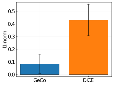
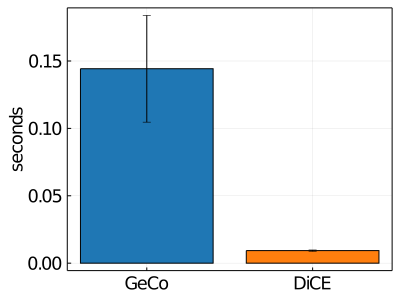
Figure 5. Comparison of the average distance and runtime of GeCo and DiCE for a neural network on 5000 Adult instances. Error bars represent one standard deviation.

Takeaways for Evaluation with Neural Net. Figure 5 presents the key results for our evaluation on the MLP classifier. We only show the comparison of GeCo and DiCE, because the comparison with WIT, SimCF, and CERT is similar to the one for decision trees. MACE requires an extensive conversion of the classifier into a logical formula, which is not supported for the considered model.

Since DiCE computes the counterfactual explanation in one pass over a variational auto-encoder, it is able to compute the explanations very efficiently. In our experiments, DiCE was able to find an explanation on average $15.5\times$ faster than GeCo. The counterfactuals that DiCE generates, however, have poor quality. Whereas GeCo is again able to find explanations with only few required changes, DiCE changes on average 5.3 features. As a result, GeCo’s explanation is on average $4.4\times$ closer to the original instance. Therefore, we consider GeCo much more suitable for real-world applications.

Allstate Dataset w. Random Forest     Yelp Dataset w. Random Forest     Yelp Dataset w. MLP (small)       Yelp Dataset w. MLP (large)

[]

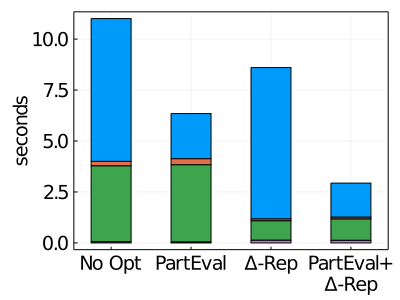
Figure 6. Breakdown of GeCo’s runtime into the main operators on Allstate and Yelp using random forest and MLP classifiers. We present the runtimes (1) without the $\Delta$-representation and partial evaluation, (2) with partial evaluation, (3) with the $\Delta$-representation, and (4) with both optimizations. The runtime is averaged over 1,000 instances.

Table 3. Microbenchmarks results for tree-based models.

	Credit	Adult	Allstate	Yelp
Generations	4.22	4.66	5.26	3.24
Explored Candidates	18.1K	15.3K	62.8K	42.9K
Size of Naive Rep.	62.23K	117.41K	8.03M	7.84M
Size of $\Delta$-Rep.	18.64K	21.88K	412K	131K
Compression	3.3$\times$	5.4$\times$	19.5$\times$	60.1$\times$

6.4. Microbenchmarks

In this section, we present the results for the microbenchmarks.

Breakdown of GeCo’s Components. First, we analyze the runtime of each operator presented in Sec. 4, as well as the impact of the $\Delta$-representation and partial evaluation (Sec. 5) on two tree-based models over Allstate and Yelp, as well as the small and large multi-layered perceptrons (MLP) over Yelp. We run GeCo for 5 generations on 1,000 instances that have been classified as bad.

Figure 6 presents the results for this benchmark. Initial population captures the time it takes to compute the feasible space, and to generate and select the fittest candidates for the initial population. The times for selection, crossover, and mutation are accumulated over all generations. For each scenario, we first present the runtime for: (1) without the $\Delta$-representation and partial evaluation enabled, (2) with each optimization individually, and (3) with both.

The results show that the selection and mutation operators are the most time consuming operations of the genetic algorithm. This is not surprising since they operate on tens of thousands of candidates, whereas crossover combines only a few selected candidates.

Partial evaluation of the classifier is effective for the random forest model. For Allstate, it decreases the runtime of the selection operator by up to 3.2$\times$, which translates into an overall speedup of $1.7\times$. For MLPs, the optimization is less effective, because we can only partially evaluate the first layer. In fact, the overhead of partial evaluation results in a slowdown for the larger variant.

The $\Delta$-representation decreases the runtime of the mutation operator by 3.9$\times$ for Allstate and $4.7\times$ for Yelp (random forest). This speedup is due to the compression achieved by the $\Delta$-representation (see below). If the classifier is not partially evaluated, then there is a tradeoff in the runtime for the selection operator, because it requires the materialization of the full feature vector. This materialization increases the runtime of selection by up to 1.6$\times$ (Yelp, MLP small).

The best performance is achieved if the $\Delta$-representation and partial evaluation of the classifier are used together. In this case, there is a significant runtime speedup for both the mutation operator and selection operators. Overall, this can lead to a performance improvement of $5\times$ (Yelp, random forest).

Figure 7. Evaluation of GeCo over 100 Credit instances with synthetic classifiers that require 1-12 feature changes. (left) Average runtime and number of generations; (right) Average distance of GeCo compared to the optimal explanation.

Validating Explanation Quality. To evaluate whether GeCo is able to find good explanations, we design synthetic classifiers for which the optimal explanation is known. Each classifier is a conjunction of unary threshold conditions, and the outcome is positive iff all conditions are satisfied. Given an instance that fails all conditions, the number of conditions is equal to the number of features that the counterfactual needs to change. We present further details on the synthetic classifiers in Appendix A.3.

Figure 7 presents the results of our evaluation on 100 Credit instances which fail all conditions for all classifiers. We consider classifiers with up to 12 conditions, which is the maximum number of features that can be changed. We add features in the decreasing order of their domain sizes, which is the most challenging order for GeCo; we consider a different order in Appendix A.3.

GeCo always finds a valid counterfactual explanation, even if we require changing all 12 features. The runtime is linear with respect to the number of features changed, and proportional to number of generations of the genetic algorithm. The distance of the explanations is always close to the distance of the optimal explanation. In Appendix A.3, we show that, by sampling more values during mutation, we can further decrease the distance gap to the optimal explanation with minor performance degradation.

Number of Generations and Explored Candidates. Table 3 shows for each dataset how many generations GeCo needed on average to converge, and how many candidates it explored. The majority (up to 97%) of the candidates were generated by mutate.

Compression by $\Delta$-representation. Table 3 compares the sizes for the naive listing representation and the $\Delta$-representation. We measure size in terms of the number of represented values, and take the average over all generations for the size of the candidate population after the mutate and crossover operations. Overall, the $\Delta$-representation can represent the candidate population up to $60\times$ more compactly than the naive listing representation.

Effect of Constraints. We evaluate the impact of the PLAF constraints on GeCo’s runtime. The constraints without implications significantly restrict the search space of feasible counterfactuals. Thus, including these constraints improves the performance by 19.3% for Adult and 32.2% for Credit. The constraints with implications, however, may introduce some overhead since they need to be checked dynamically using action cascading. For example, the overhead is 19.2% for Adult and 32.3% for Credit. Yet, the version with all constraints is still faster by 9.8% for Credit and 18.7% for Adult over the version without any constraints. Finally, the grouping of features also restricts the search space. For Adult, GeCo is 1.4$\times$ faster using the feature groups than without.

7. Conclusions

We described GeCo, the first interactive system for counterfactual explanations that supports a complex, real-life semantics of counterfactuals, yet provides answers in real time. GeCo defines a rich search space for counterfactuals, by considering both a dataset of example instances, and a general-purpose constraint language. It uses a genetic algorithm to search for counterfactuals, which is customized to favor counterfactuals that require the smallest number of changes. We described two powerful optimization techniques that speed up the inner loop of the genetic algorithm: $\Delta$-representation and partial evaluation. We demonstrated that, among five other systems reported in the literature, GeCo is the only one that can both compute quality explanations and find them in real time.

This work opens up several directions for future work. First, counterfactual explanations are subject to updates to the underlying data and classifier. We plan to explore how we can generate explanations that are robust to small changes in the data distribution or classifier. This is related to the more general problem of robust machine learning. Second, GeCo requires that the PLAF constraints are provided by a domain expert. We plan to explore how we can leverage constraints and dependencies in databases to generate these constraints automatically. Third, GeCo currently assumes that the input to the model is the raw data. In practice, however, the model input is typically the output of extensive feature engineering. We plan to explore how GeCo can generate explanations for the feature engineered data, but then return the corresponding raw data values to the user. For structured relational data, the feature engineering involves aggregating the raw data, in which case we would have to connect GeCo with techniques on explaining aggregate queries that have been developed in the database community. Fourth, counterfactual explanations expose values from the database, which may lead to privacy issues. We plan to explore how to return explanation that satisfy both privacy and legislative requirements. Finally, we have implemented partial evaluation manually, and it is only supported for random forests and simple neural network classifiers. We plan to extend this optimization to other models by leveraging work from the compilers community.

Appendix A Additional Experiments

In this section, we present further details and extensions for the experiments presented in Sec. 6.

A.1. Constraints

We present the PLAF constraints used in the experiments in Sec. 6. Figure 8 presents the constraints we considered for the Credit and Adult datasets.

For Adult, we enforce that Age and Education can only increase, and MaritalStatus, Relationship, Gender, and NativeCountry cannot change. The implication specifies that if Education increases then Age needs to increase as well. The Adult dataset has two features that describe the education level, EducationNumber and EducationLevel. Since these two features are clearly correlated, we group them into a single feature group. For the experiments in Sec. 6.2 we restrict the number of hours worked per week to at most 60, since it is unrealistic to assume that the considered instance will exceed this limit.

For Credit, we enforce that AgeGroup, EducationLevel, and HasHistoryOfOverduePayments can only increase, while isMale and isMarried cannot change. The first implication specifies that an increase in education level for a teenaged customer results in an increase in the AgeGroup from teenager to adult. The second implication specifies that if the number of months with low spending in the last 6 months increases then the number of months with high spending in the last 6 months should decrease.

For Yelp, we define a total of 18 constraints which specify that (1) the location of a business cannot change (i.e., city, state, longitude, and latitude are immutable) and (2) past reviews cannot be deleted (i.e., the review count or the number of compliments for businesses cannot decrease). In addition, we synthesis two constraints with implications. The first implication specifies that if the review count for a business increases, then the business must be open. The second implication states that if a review receives more “cool” tags, then we expect the business to also receive more “cool” compliments.

[] Adult Dataset PLAF x_cf.Age >= x.Age PLAF x_cf.Education >= x.Education PLAF x_cf.MaritalStatus = x.MaritalStatus PLAF x_cf.Relationship = x.Relationship PLAF x_cf.Gender = x.Gender PLAF x_cf.NativeCountry = x.NativeCountry PLAF IF x_cf.Education > x.Education          THEN x_cf.Age >= x.Age+4 Credit Dataset PLAF x_cf.isMale = x.isMale PLAF x_cf.isMarried = x.isMarried PLAF x_cf.AgeGroup >= x.AgeGroup PLAF x_cf.EducationLevel >= x.EducationLevel PLAF x_cf.HasHistoryOfOverduePayments >=          x.HasHistoryOfOverduePayments PLAF x_cf.TotalOverdueCounts >= x.TotalOverdueCounts PLAF x_cf.TotalMonthsOverdue >= x.TotalMonthsOverdue PLAF IF x_cf.EducationLevel > x.EducationLevel+1          && x.AgeGroup < 2 THEN x_cf.AgeGroup == 2 PLAF IF x_cf.MonthsWithLowSpendingLast6Months >          x.MonthsWithLowSpendingLast6Months          THEN x_cf.MonthsWithHighSpendingLast6Months <          x.MonthsWithHighSpendingLast6Months

Figure 8. PLAF constraints used for Adult and Credit.

A.2. Number of Features Changed

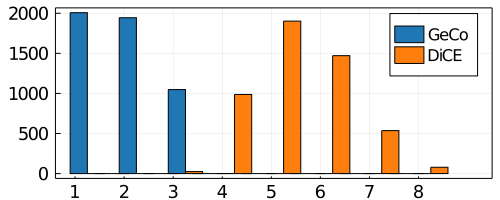
Figure 9. Distribution of number of features changed by GeCo and DiCE on 5000 Adult instances.

[]

Credit Dataset	Adult Dataset

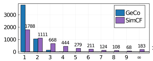
Figure 10. Distribution of the number of features changed by GeCo, MACE, WIT, CERT, and SimCF on Credit and Adult.

[]

The experiments in Sec. 6.3 showed that GeCo is able to find explanations that are closer to the original instance than the five competing systems. This can be attributed to the fact that GeCo is able to find counterfactual explanations that require changing fewer features. Figure 10 presents the distribution of the number of features changed by MACE, WIT, CERT, and SimCF in comparison with the number of features changed by GeCo. For the Credit dataset, for instance, GeCo can find explanations with 1.27 changes on average, while MACE (the best competitor) changes on average 3.39 features. WIT, CERT, and SimCF change on average 3.97, 3.15, and respectively 2.98 features.

Figure 9 presents the corresponding distribution from the comparison with DiCE. The plot shows again that GeCo is able to find explanations with few changes (1.8 changes on average), whereas DiCE changes on average 5.4 features which is more than half of the total number of features that can be changed.

A.3. Synthetic Classifiers

In this section, we present further details on the experiments with synthetic classifiers for which we know the optimal explanation.

Details on Classifiers. Each classifier is a conjunction of unary threshold conditions (e.g. MostRecentBillAmount >= 4020.0). This allows us to reason about the optimal explanations for any instance that fails the threshold conditions. For example, if the condition is MostRecentBillAmount <= 4020.0, then the minimum change for any instance that fails this condition would be to set MostRecentBillAmount = 4020.0. The classifier returns 1 (the positive outcome) if and only if all conditions are satisfied; otherwise we return $0.5-d$, where $d$ denotes the normalized distance between the candidate and the optimal explanation.

In Sec.6.4, we consider the following threshold conditions for the mutable features of the Credit dataset:

1. MaxBillAmountOverLast6Months >= 4320.0

2. MostRecentBillAmount >= 4020.0

3. MaxPaymentAmountOverLast6Months >= 3050.0

4. MostRecentPaymentAmount >= 1220.0

5. TotalMonthsOverdue >= 12.0

6. MonthsWithZeroBalanceOverLast6Months >= 1.0

7. MonthsWithLowSpendingOverLast6Months >= 1.0

8. MonthsWithHighSpendingOverLast6Months >= 3.0

9. AgeGroup >= 2.0

10. EducationLevel >= 3.0

11. TotalOverdueCounts >= 1.0

12. HasHistoryOfOverduePayments >= 1.0

We design 12 synthetic classifiers, where each classifier adds an additional condition in the order shown above. For instance, the first classifier only checks if MaxBillAmountOverLast6Months >= 4320.0, the second checks if MaxBillAmountOverLast6Months >= 4320.0 && MostRecentBillAmount >= 4020.0, and so on. The order in which the conditions are presented to the classifier is the reverse order with respect to the size of their feature domains. This is the most challenging order for GeCo because it is more difficult to find the best counterfactual when searching large domain spaces.

During the evaluation we consider only instances that fail all threshold conditions in the classifier, which means that the counterfactual needs to change at least as many features as there are conditions in the classifier.

Figure 11. Comparison of two variants of GeCo using the synthetic classifiers over Credit. The first variant uses the default number of samples during mutation, and the second variant samples $5\times$ more values.

[]

Evaluation with more samples. In Sec.6.4, we show that, for the evaluation with synthetic classifiers, GeCo is always able to find a valid counterfactual explanation. However, as shown in Fig.7, GeCo may not always find the optimal explanation. This is due to the fact that we are exploring large domain sizes, and the sampling of action may not sample the optimal action for each feature. To mitigate the gap in the distance between GeCo’s explanation and the optimal explanation we can increase the number of samples during mutation.

The experiments in Fig.7 assumed the default settings for the number of samples during mutation $(\texttt{m}_{\text{init}}=20,\texttt{m}_{\text{mut}}=5)$. In Fig.11 we compare two variants of GeCo. The first variant assumes the default settings, and the second samples five times more values during mutation $(\texttt{m}_{\text{init}}=100,\texttt{m}_{\text{mut}}=25)$. The results show that the increase in the number of samples lowers the gap in distance between GeCo’s explanation and the optimal explanation. This, however, comes with a performance degradation since the increase in the number of samples requires GeCo to evaluate the classifier on more candidates. Even though we are sampling $5\times$ more values, the performance is only $2\times$ slower for the classifier that requires changing all twelve features.

Evaluation with different feature order. In the previous sections, we designed the synthetic classifiers following the decreasing order of the feature domain sizes. Fig.12 presents the same evaluation using the following order, where we interleave features with large and small domain sizes (using the same threshold values):

1. MaxBillAmountOverLast6Months,

2. TotalOverdueCounts,

3. MostRecentBillAmount,

4. AgeGroup,

5. MaxPaymentAmountOverLast6Months,

6. HasHistoryOfOverduePayment,

7. MostRecentPaymentAmount,

8. TotalMonthsOverdue,

9. EducationLevel,

10. MonthsWithZeroBalanceOverLast6Months,

11. MonthsWithLowSpendingOverLast6Months,

12. MonthsWithHighSpendingOverLast6Months.

Figure 12. Evaluation of GeCo over 100 Credit instances with the synthetic classifiers that require 1-12 feature changes. We add features one at a time using an order that interleaves features with large and small domain sizes. (left) Average runtime and number of generations; (right) Average distance of GeCo compared to the optimal explanation.

[]

The results are comparable to Fig.7: the runtime depends to the number of generations of the genetic algorithm, and the distance is consistently close to one of the optimal explanation. The runtime plot, however, is not a linear curve, because GeCo finds explanations easier if we add a condition for a feature with small domain size. For instance, adding AgeGroup in experiment 4 has no significant effect on the runtime, because the dataset contains only 5 age groups.

A.4. Effect of Distance Function

Recall our distance function from Eq. (2) and its parameters $\alpha,\beta,\gamma$. In Sec. 6.3, we show the explanation quality for GeCo on Credit and Adult using the parameters $(\alpha=0,\beta=1,\gamma=0)$. When setting $(\alpha=0.5,\beta=0.5,\gamma=0)$ and $(\alpha=0.33,\beta=0.34,\gamma=0.33)$, we observe that using the $\ell_{0}$-norm ($\alpha>0$) further reduces the number of features that GeCo changes. In this case, GeCo always returns explanations that change only a single feature, for both Credit and Adult. This is because GeCo can find explanations with a single change, but the magnitude of this change may be larger than that of changing multiple features. Thus, the user should only include the $\ell_{0}$-norm if the goal is to limit the number of features changed. The $\ell_{\infty}$-norm has no significant effect in our experiments, which may be because the $\ell_{1}$-norm already restricts the maximum change.

We observed that including $\ell_{0}$-norm decreases the number of features changed also in the experiments with synthetic classifiers. When we consider the setting $(\alpha=0,\beta=1,\gamma=0)$, it is possible that GeCo changes more features than necessary. For instance, for experiments 1-4, GeCo changes on average 1.7, 2.9, 3.7, and respectively 4.4 features. When we use $(\alpha=0.5,\beta=0.5,\gamma=0)$, however, GeCo always changes only the number of features that are required, because the $\ell_{0}$-norm enforces a penalty on changing additional features. For the experiments that require five or more feature changes, there is no difference in then number of features changed between the two settings. In these experiments, GeCo is required to run more generations and thus automatically explores more combinations.