A cuspy dark matter halo

Abstract

The cusp-core problem is one of the main challenges of the cold dark matter paradigm on small scales: the density of a dark matter halo is predicted to rise rapidly toward the center as $\rho(r)$ $\propto$ $r^{\alpha}$ with $\alpha$ between -1 and -1.5, while such a cuspy profile has not been clearly observed. We have carried out the spatially-resolved mapping of gas dynamics toward a nearby ultra-diffuse galaxy (UDG), AGC 242019. The derived rotation curve of dark matter is well fitted by the cuspy profile as described by the Navarro-Frenk-White model, while the cored profiles including both the pseudo-isothermal and Burkert models are excluded. The halo has $\alpha$= -(0.90$\pm$0.08)  at the innermost radius of 0.67 kpc , $M_{\rm halo}$=(3.5$\pm$1.2)$\times$10¹⁰ M_⊙  and a small concentration of 2.0$\pm$0.36. AGC 242019 challenges alternatives of cold dark matter by constraining the particle mass of fuzzy dark matter to be $<$ 0.11$\times$10^-22 eV  or $>$ 3.3$\times$10^-22 eV , the cross section of self-interacting dark matter to be $<$ 1.63 cm²/g, and the particle mass of warm dark matter to be $>$ 0.23 keV, all of which are in tension with other constraints. The modified Newtonian dynamics is also inconsistent with a shallow radial acceleration relationship of AGC 242019. For the feedback scenario that transforms a cusp to a core, AGC 242019 disagrees with the stellar-to-halo-mass-ratio dependent model, but agrees with the star-formation-threshold dependent model. As a UDG, AGC 242019 is in a dwarf-size halo with weak stellar feedback, late formation time, a normal baryonic spin and low star formation efficiency (SFR/gas).

1 Introduction

The cosmological model of cold dark matter and dark energy, i.e., $\Lambda$CDM, has achieved tremendous success in understanding the cosmic structure across time on large scales, but this model is challenged by observations on small scales such as the cusp-core problem, the missing dwarf problem, the too-big-to-fail problem etc. (for a review, see Weinberg et al., 2015).

In cosmological simulations of cold and collisionless dark matter, a dark matter halo has a density profile that rises toward the center with a power index of -1 to -1.5 (Moore, 1994; Burkert, 1995; Navarro et al., 1997; Moore et al., 1998; Ghigna et al., 2000; Jing & Suto, 2002; Wang et al., 2020), referred as a cuspy profile. However, over the past decades, much shallower or even flat core-like profiles toward centers have been found in most, if not all, observed data of nearby galaxies through mapping dynamics of gas and stars. Early studies with HI interferometric data reveal shallow dark-matter central profiles in individual galaxies (Carignan & Beaulieu, 1989; Lake et al., 1990; Jobin & Carignan, 1990). Studies with higher spatial resolutions for a larger sample of dwarfs and low-surface-brightness galaxies further confirm the central flatness of the rotation curve, and derived a median dark-matter density slope of about -0.2 toward centers (de Blok et al., 2001; Oh et al., 2011, 2015). Optical observations of ionized gas such as H$\alpha$  can achieve higher spatial resolutions than the HI data, and confirmed the median density slope of about -0.2 with long-slit spectra for a large sample of dwarf galaxies (Spekkens et al., 2005). Although the rotation curves from the long-slit spectroscopic data are sensitive to the assumed dynamical center, the position angle of the kinematic major axis etc, further studies with optical integral field unit have suggested insignificance of the above effects and validated dark-matter profiles with central shallower slopes (Kuzio de Naray et al., 2008; Adams et al., 2014).

Among few galaxies whose halos can be described by cuspy profiles, the one with the highest signal-to-noise-ratio is DDO 101 that has a central dark-matter slope of -1.02$\pm$0.12 (8.5-$\sigma$) (Oh et al., 2015). However, this object can be fitted equally well with a cored profile; the difference in the reduced $\chi^{2}$ is only 0.02 for a degree of freedom (d.o.f) of six (see Oh et al., 2015). This is because of the limitation on the spatial resolution and spatial extent of the observed rotation curve, as well as different models for cuspy and cored profiles (see § 3.2). For example, the density slope of a NFW model for a cuspy profile varies from -1 at the center to -3 at infinity, while the pseudo-isothermal (ISO) model for a cored profile has a slope from 0 at the center to -2 at infinity, so that both models may perform well on fitting the data with a limited spatial extent. In order to identify a definitive cuspy dark matter halo, it is thus required to demonstrate not only the validity of cuspy models but also the invalidity of cored models. For DDO 101, the large uncertainty in its distance further challenges the reliability of its cuspy profile (Read et al., 2016b). Studies of local dwarf spheroidal galaxies also suggest cuspy profiles in few objects, among which the highest-probability one is Draco with a central density slope of -1.0 at 5.0-$\sigma$ and 6.8-$\sigma$ by Jardel et al. (2013) and Hayashi et al. (2020), respectively. However, it has not been demonstrated whether a cored model can fit the data or not for this object, as done for DDO 101. And furthermore, systematic uncertainties are complicated for these studies in which the velocity dispersion among individual stars as a function of the galactic radius are used to measure the dark matter distribution. The orbital anisotropy, the method to model stellar orbits, the dark-matter shape and the limited number of the member stars are all found to affect the conclusions (Evans et al., 2009). Especially, a recent study of simulated galaxies by Chang & Necib (2020) emphasized the importance of a large amount of stars in order to unambiguously measure the dark matter distribution. If the number of stars is less than 10000, an intrinsic cored profile cannot be differentiated reliably from a cuspy profile. For Draco, there are only $\sim$468 member stars (Walker et al., 2015). Fortunately, these systematic uncertainties are significantly eliminated for HI interferometric data as seen in simulated galaxies (Kuzio de Naray et al., 2009; Kuzio de Naray & Kaufmann, 2011). This is mainly because gas is collisional and their dynamics can be relatively easily described by titled-ring models (Begeman, 1989; Di Teodoro & Fraternali, 2015). In summary, the above few claimed cuspy profiles of dark halos are not definitive.

There are two solutions to the small scale controversies of $\Lambda$CDM. One is to modify the nature of dark matter so that it is no longer cold but instead self-interacting, fuzzy or warm. These modifications can retain the properties of the universe on large scales as predicted by $\Lambda$CDM but resolve its small-scale challenges. Fuzzy cold dark matter, also known as ultralight scalar particles, has a mass around 10^-22 eV (e.g. Hu et al., 2000; Schive et al., 2014). The uncertainty principle of its wave nature acts on kpc scales, smoothing the density fluctuations and preventing the growth of small halos and formation of central cusps. The self-interacting dark matter transports “heat” (higher velocity dispersion) from the outer region to the “cooler” inner region of a halo. It leads to a constant density core with isothermal velocity dispersion (e.g. Spergel & Steinhardt, 2000; Rocha et al., 2013; Tulin & Yu, 2018). If dark matter is warm, it decouples from the primordial plasma at relativistic velocity, thus free streaming out of small density peaks. As a result, the structure formation at small scales are suppressed (e.g. Avila-Reese et al., 2001; Lovell et al., 2014). Warm dark matter scenario is found to have a “catch-22” problem, i.e., if the “cusp-core” problem is resolved, the requirement for the particle mass cannot form small galaxies at the first place, and vice versa (e.g. Macciò et al., 2012).

Another solution is to keep cold dark matter paradigm but invoke efficient gravitational interaction between dark matter and baryonic matter through stellar feedback (Navarro et al., 1996; Governato et al., 2010). Overall, as gas falls into the inner region of the halo, star formation takes place and the subsequent feedback through supernovae expels an appreciable amount of gas and stars to large radii. These baryonic matter pulls dark matter particles to migrate outward through pure gravitational interaction, lowering the central density of dark matter. The overall efficiency of this interaction and its effects are still under investigations (Di Cintio et al., 2014; Read et al., 2016a; Tollet et al., 2016; Bose et al., 2019; Benítez-Llambay et al., 2019; Read et al., 2019). In addition to the stellar feedback, other mechanisms have also been proposed, such as dynamical friction between gas clouds and dark matter particles (Nipoti & Binney, 2015).

A definitive cuspy profile from observations will prove the validity of the cold dark matter paradigm on subgalactic scales while challenging other types of dark matter. As shown in Figure 1, the object AGC 242019 is an ultra-diffuse galaxy (UDG) identified by the Arecibo Legacy Fast ALFA (ALFALFA) survey of Hi  galaxies (Leisman et al., 2017). This galaxy has a stellar mass of (1.37$\pm$0.05)$\times$10⁸ M_⊙ , a HI mass of (8.51$\pm$0.36)$\times$10⁸ M_⊙  and a star formation rate of (8.2$\pm$0.4)$\times$10^-3 M_⊙ yr^-1  as listed in Table 1. Its receding velocity is 2237$\pm$25 km s^-1 after correcting for the Virgo, Great Attractor and Shapley supercluster (Mould et al., 2000). In the cosmological frame of $h$=0.73, $\Omega_{0}$=0.27 and $\Omega_{\Lambda}$=0.73, the corresponding distance is 30.8 Mpc and the uncertainty is estimated to be 5%, given that it is an isolated field galaxy (see § 4.2).

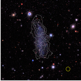
Figure 1: False-color image of AGC 242019. The false-color image of the $g$, $r$ and $z$ bands. The white contours of the Hi  intensity are at levels of 0.4, 0.6 and 0.8 mJy km s^-1. The yellow ellipse indicates the Hi  beam size.

Figure 2: The HI data of AGC 242019. a, The Hi  intensity. b, The integrated spectra of the VLA compared to the Arecibo’s spectrum (Haynes et al., 2018). c, The radial profile of the gas mass surface density corrected for inclination and helium.

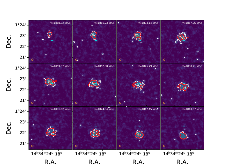
Figure 3: The channel map of the Hi  data. The contour levels are 1, 3, 4.5 and 6 mJy km s^-1. The white and red contours indicate the observations and best-fitted models, respectively.

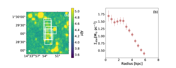
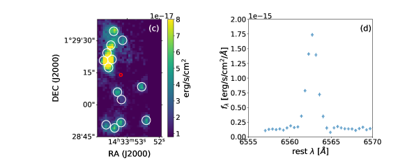
Figure 4: The infrared and optical data of AGC 242019. a, The 3.6 $\mu$m flux density with overlaid WiFeS IFU pointings. b, The radial profile of the stellar mass surface density corrected for the inclination. c, Individual H$\alpha$ clumps for which the line of sight velocities are measured. Each clump has a circular radius of 2.0$\arcsec$. The small red circle indicates the dynamical center. d, The integrated spectrum of H$\alpha$ emissions.

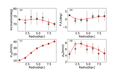
Figure 5: The two-stage operation of ^3DBarolo. The gray points are the first stage, where four parameters of each ring are set as free. The red points are the second stage, where the inclination and position angles are regularized by fitting a Bezier function to the results from the first stage.

2 Observations and data reduction

2.1 Radio interferometric observation of Hi  gas with the VLA

Our L-band observations were performed with the Karl G. Jansky Very Large Array (VLA) through two projects corresponding to the D configuration (19B-072; PI: Y. Shi) and to the C and B configurations (20A-004; PI: Y. Shi). The D-configuration observations were performed on 21 and 23 Sep. 2019, each with a 1.5-hr observing time and a $\sim$ 66 min on-source time. A total of 27 antennas were employed in both executions, with the first under overcast weather conditions and the second under clear weather conditions. The projected baselines of the D-configuration array are in the range of 34–1050 m. The flux and bandpass calibrator was 3C 295, and the gain calibrator was J 1419+0628. We configured the spectrometers with a mixed setup. The spectral line window that covers the Hi 21-cm line has a bandwidth of 128 MHz and a channel width of 32.3 kHz ($\sim$ 6.9 km s^-1), while the remaining windows cover a frequency range between 963.0 MHz and 2017.0 MHz to optimize the sensitivity for the radio continuum.

The C-configuration observations were performed on 04, 09 and 13 Feb. 2020, each with a 2-hr observing time and a $\sim$ 90 min on-source time. Two observations were conducted with 25 antennas, while the rest were observed with 26 antennas, mostly under overcast or clear weather conditions. The projected baselines of the C configuration are in the range of 40–3200 m. In the C-configuration observations, the 21-cm emission line was observed with a spectral line widow that has a channel width of 5.682 kHz ($\sim$ 1.2 km s^-1) and a bandwidth of 32 MHz. The remaining windows cover a frequency range between 963.0 MHz and 2017.0 MHz, for optimizing the radio continuum bandwidth. The flux and bandpass calibrator was 3C 286 and the gain calibrator was J 1419+0628.

The B-configuration observation was performed with five executions during July and August of 2020, each with a 2-hr observing time and a $\sim$ 90 min on-source time. In most executions, 27 antennas were employed under cloudy conditions. The projected baselines of the B-configuration are in the range of 230–11000 m. The hardware setup and the calibrators were the same as those used for the C-configuration observations.

We reduced all data manually with the Common Astronomy Software Applications (CASA) package (McMullin et al., 2007), v5.6.1. Both D-configuration observations were severely affected by radio frequency interferences (RFI). Therefore we calibrated and flagged the data manually. Approximately 20% of the data have to be flagged, across different frequency ranges. The data obtained on 21 Sep. 2019, including the calibrators, has about three times higher noise than that estimated from the VLA sensitivity estimator, due to unknown reasons. However, the fluxes, line profile, and spatial distributions are highly consistent with the data obtained on 23 Sep. 2019. Whether combine it to the final data does not change the results. All gain calibrators were checked carefully to ensure a flat bandpass, a point-source distribution and excellent calibration solutions. The 1.4 GHz flux densities of 3C 286, 3C 295 and J 1419+0628 were 15.1$\pm$0.1 Jy, 22.3$\pm$0.1 Jy, and 6.0$\pm$0.1 Jy.

After flagging and calibration, we weighted all dataset with their noise levels using the statwt task. Then, through the uvcontsub task, we fitted and subtracted the radio continuum from the visibility data, with line-free channels on both sides of Hi, using the first-order linear function. We resampled the C- and B-array data to match with the spectral resolution of the D-array data, using the mstransform task. The final spectrally matched line-only data from the D, C, and B configurations were combined together with the concat task.

In the end, we inverted the visibility data to the image plane and cleaned the data cube with Briggs’ robust parameter of 2.0 using the tclean task. The final D+C+B datacube has a velocity coverage of 500 km s^-1  and a channel width of 32 kHz, corresponding to a velocity resolution of $\sim$ 7 km s^-1. The r.m.s. noise level reaches 0.26 mJy beam^-1 per channel with a restoring synthesis beam size of 9.85^′′ $\times$9.33^′′ and a position angle of 17.56^∘.

The Hi  intensity map is shown in Figure 2 (a). The integrated spectrum of the B+C+D configuration has a flux of 3.8$\pm$0.16  Jy km s^-1, which is comparable to the flux of 3.4 Jy km s^-1  obtained with the Arecibo (Leisman et al., 2017), as shown in Figure 2 (b). The total HI gas mass is (8.51$\pm$0.36)$\times$10⁸ M_⊙ . A slightly higher flux as seen by VLA in the red wing may be caused by a small offset of the Arecibo beam from the galaxy center, given a large size of the galaxy that is two arcmins in the diameter. The radial profile of the gas mass surface density is shown in Figure 2 (c). The channel map is shown in Figure 3.

We also tested tilted-ring modeling with the combined data using the B+C configurations and found essentially no difference, except for a higher noise level. Though the better velocity resolution leads to better estimates of the pressure support, which has a very minor contribution to the decomposition of the rotation curve.

2.2 Broad-band images

The co-added images at 3.6 and 4.5 $\mu$m were obtained from the Wide-field Infrared Survey Explorer (WISE) archive (Wright et al., 2010) with spatial resolutions of 6.0^′′ and 6.8^′′, respectively. The target is well detected at 3.6 $\mu$m as presented in Figure 4 (a), but shows almost no detection at 4.5 $\mu$m. To derive the radial profile of the stellar mass surface density as presented in Figure 4 (b), a few nearby bright stars in the field were subtracted using the stellar point spread functions. The stellar mass based on the 3.6 $\mu$m image is estimated to be (1.37$\pm$0.05)$\times$10⁸ M_⊙  for a Kroupa stellar initial mass function and a mass-to-light ratio $\Upsilon_{3.6{\mu}m}$=0.6 ($M_{\odot}/L_{\odot,3.6{\mu}m}$) (see below).

The optical $g$ and $r$ images were obtained from the Dark Energy Camera Legacy Surveys (Dey et al., 2019). The far-ultraviolet image was retrieved from the GALEX data archive. The integrated flux was converted to a star formation rate of (8.2$\pm$0.4)$\times$10^-3 M_⊙ yr^-1  for a Kroupa stellar initial mass function (Leroy et al., 2008).

2.3 Integral field unit observation of H$\alpha$ by ANU 2.3 m

Integral field unit observations of H$\alpha$ were carried out with the Wide-Field Spectrograph (WiFeS) onboard the Australian National University 2.3 m telescope on the nights of 21-22 Mar., 26 May and 20-22 Jul., 2020. An R7000 grism (5290-7060${\rm\AA}$) at a resolution of 7000 was adopted to cover the H$\alpha$ emission line. WiFeS has a field of view of 25$\arcsec$$\times$38$\arcsec$. As shown in Figure 4 (a), exposures were taken at several positions to cover the whole optical extent of the galaxy, with one pointing toward a nearby bright star for astrometric calibration. Each exposure was 30 mins, and the total on-source integration time varied from 2.0 hrs to 3.5 hrs at each pixel. For every 1–2 hrs, an off-target blank sky and a standard star were observed. The seeing was between 1.5^′′ and 2.0^′′. Each frame was first reduced following the standard procedure by pyWiFeS (Childress et al., 2014), and then was subtracted by the median value of the sky frame at each wavelength. Individual frames were aligned with each other to produce the final mosaic image using the positions of the H$\alpha$ clumps, as the continuum emission was too faint. The absolute astrometry was obtained through alignment with the brightest star in the mosaic field of view. Since H$\alpha$ clumps are not perfect point sources, we estimated the final astrometric uncertainty to be about 1^′′. To correct the barycentric velocity offset and any possible intrinsic instrumental shift, the wavelength solution of each night was further cross-calibrated based on H$\alpha$ lines of the same clumps observed during different nights. The integrated H$\alpha$  flux map is presented in Figure 4 (c) with the integrated spectrum shown in Figure 4 (d).

3 Data Analysis

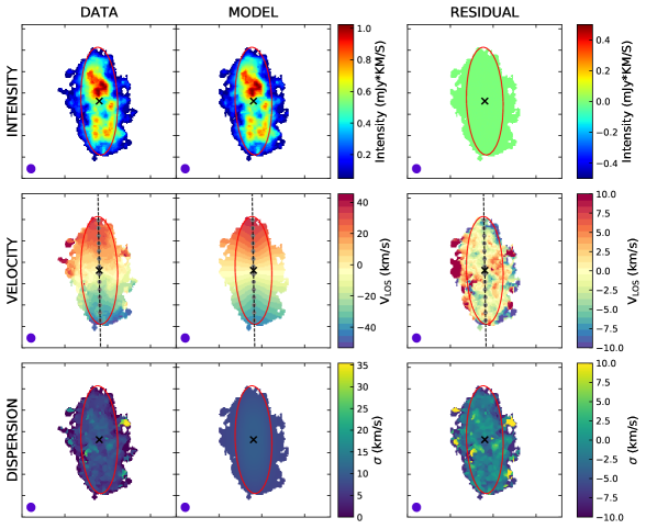
Figure 6: The moment maps and tilted-ring modeling achieved through ^3DBarolo. First row: the moment-0 map, best-fitting model and residual for the Hi  intensity. Note that the run of ^3DBarolo adopted the setting NORM=LOCAL which normalizes the model’s flux to the observed one pixel by pixel. As a result, the flux residual is zero. Second row: the moment-1 map, best-fitting model and residual for the velocity. Third row: the moment-2 map, best-fitting model and residual for the velocity dispersion. In all panels, the filled ellipse on the left lower corner indicates the beam, while the large red ellipse marks the outer boundary of the last ring.

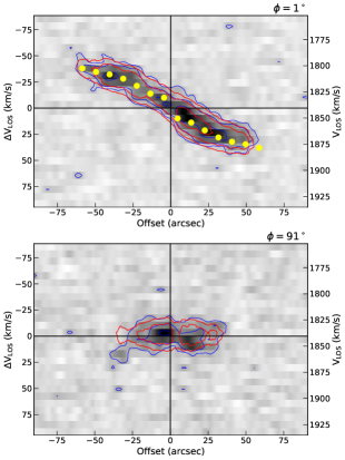
Figure 7: The position-velocity diagram of the galaxy along the major and minor axes of the Hi gas disk. The blue and red contours are the observation and best-fitted model, respectively. The yellow symbol is the derived line-of-sight velocity of each ring after correcting the beam smearing. The contour levels are 0.73, 1.44, 2.88 and 5.77 mJy km s^-1.

Table 1: The Properties of AGC 242019

Parameters	Mean	1-$\sigma$ error	3% HPD¶	97% HPD¶
$M_{\rm star}$ (10${}^{8}M_{\odot}$)	1.37	0.05	-	-
$M_{\rm HI}$ (10${}^{8}M_{\odot}$)	8.51	0.36	-	-
SFR (10-3M⊙/yr)	8.2	0.4	-	-
Dynamical center∗ (J2000)	14:33:53.38, 01:29:12.5	5.0′′, 2.2′′	-	-
$V_{\rm sys}^{\ast}$ (km s-1)	1840.4	1.9	-	-
Distance (Mpc)	30.8	5%	-	-
log($\Upsilon_{3.6{\mu}m}$ ($M_{\odot}/L_{\odot,3.6{{\mu}m}}$))	-0.22	0.1	-	-
$R_{200}$ (NFW) (kpc)	65.0	7.4	54.6	74.3
$R_{\rm S}$ (NFW) (kpc)	33.3	9.1	17.4	50.6
concentration (NFW)	2.0	0.36	1.45	2.72
$M_{\rm halo}$ (NFW) (10${}^{10}M_{\odot}$)	3.5	1.2	1.5	5.8
$V_{\rm norm}$ (ISO) (km s-1)	16.7	1.9	13.1	20.3
$R_{\rm C}$ (ISO) (kpc)	2.5	0.5	1.6	3.3

Table 2: The results of the tilted-ring modeling

Rad	$V^{\rm rot}_{\rm obs}$	$V^{\rm circ}_{\rm obs}$	$\sigma^{\rm disp}$	$V^{\rm circ}_{\rm gas}$	$V^{\rm circ}_{\rm star}$	$V^{\rm circ}_{\rm dark{\textendash}matter}$	P.A.	Inclination
(kpc)	(km s-1)	(km s-1)	(km s-1)	(km s-1)	(km s-1)	(km s-1)	(∘)	(∘)
HI
0.67	10.4$\pm$1.2	10.6$\pm$1.2	4.5$\pm$1.3	0.2$\pm$1.2	1.9$\pm$0.5	10.4$\pm$1.2	2.6	73.0
2.02	14.5$\pm$1.3	15.5$\pm$1.2	7.7$\pm$1.3	4.1$\pm$0.4	4.5$\pm$0.3	14.2$\pm$1.4	0.3	72.5
3.36	22.3$\pm$1.4	23.5$\pm$1.3	7.7$\pm$1.0	8.2$\pm$0.3	8.3$\pm$0.4	20.4$\pm$1.5	-0.2	73.1
4.71	29.4$\pm$1.8	30.7$\pm$1.7	7.0$\pm$1.6	11.3$\pm$0.3	10.4$\pm$0.5	26.6$\pm$1.9	0.2	73.2
6.06	33.8$\pm$1.6	35.0$\pm$1.5	6.5$\pm$1.6	15.0$\pm$0.3	10.6$\pm$0.3	29.9$\pm$1.8	1.0	72.4
7.40	36.5$\pm$1.6	37.5$\pm$1.6	5.8$\pm$1.6	19.1$\pm$0.4	10.1$\pm$0.3	30.6$\pm$1.9	1.7	71.2
8.75	40.4$\pm$2.0	40.9$\pm$2.0	4.6$\pm$1.6	22.4$\pm$0.5	9.6$\pm$0.4	32.8$\pm$2.5	1.9	70.2
H$\alpha$
1.51		16.8$\pm$1.6		2.5$\pm$0.7	3.5$\pm$0.4	16.2$\pm$1.7
2.78		22.2$\pm$1.3		6.7$\pm$0.3	6.9$\pm$0.4	20.0$\pm$1.4
3.45		24.2$\pm$0.8		8.4$\pm$0.3	8.4$\pm$0.4	21.0$\pm$1.0
4.54		29.6$\pm$2.2		10.9$\pm$0.3	10.3$\pm$0.5	25.6$\pm$2.5

3.1 The derivation of the rotation curve of dark matter

We derived the rotation curve of the dark matter by first obtaining the total rotation curve from the Hi  and H$\alpha$ data with a correction for the pressure support, and then quadratically subtracting the gas and stellar gravity contributions as detailed below.

3.1.1 The observed rotation curve from titled-ring fitting to the Hi  datacube

We fitted the tilted-ring model to the Hi  3-D datacube with ^3DBarolo (Di Teodoro & Fraternali, 2015) to obtain the rotation curve as listed in Table 2. The radial width of each ring is set to be 9^′′, which is roughly the beam size so that each ring is independent. We adopted uniform weighting (WFUNC=0) and least-squared minimization (FTYPE=1). All other optional parameters are set as default. The full list of the set-up is included in Table 6.

The angular resolution and the signal-to-noise ratio were good enough to set the rotation velocity, the velocity dispersion, the position angle and the inclination angle as free parameters for each ring. Before running this setup, we first ran a model by also setting the dynamic center and the systematic velocity as free parameters, and then fixed them to the mean values of all rings as listed in Table 1.

The scale height was fixed to 100 pc, independent of the radius. If the height is varied by a factor of five (see below), the conclusion remains unchanged. We do notice that ^3DBarolo is not able to remove effects fully due to the disk height for a thick disk (Iorio et al., 2017). When running ^3DBarolo, we adopted the “twostage” fitting method, which allows a second fitting stage after regularizing the first-stage parameter sets. As shown in Figure 5, the radial profiles of the inclination and position angles from the first-stage fitting are regularized by fitting a Bezier function, based on which the second-stage fitting is performed. The errors of the derived rotation velocity and velocity dispersion in ^3DBarolo (Di Teodoro & Fraternali, 2015) are estimated through a Monte Carlo method. We also ran ^3DBarolo with only the receding and approaching sides, respectively. The velocities from three runs are within 1-$\sigma$ errors, while the velocity dispersions are also within errors except for the innermost radius, which is shown in Figure 17 of Appendix. As shown in Figure 5, the derived rotation velocity and velocity dispersion vary well within the 1-$\sigma$ error bars before and after regularization.

As shown in Figure 6, within the outer boundary of the last ring, the residual of the Hi  intensity is dominated by the observed flux noise, and the residuals of the velocity and velocity dispersions show small amplitudes with medians of 1.9 km s^-1  and 1.8 km s^-1, respectively. Figure 7 further shows the position-velocity diagram along the major and minor axes. Overall, the observation matches the best-fitted model well.

As gas is collisional, pressure support is a driver of gas motion in addition to gravity (Bureau & Carignan, 2002; Oh et al., 2015; Iorio et al., 2017; Pineda et al., 2017). A gas disk in equilibrium satisfies:

$$V_{\rm circ}^{2}=V_{\rm rot}^{2}+V_{\rm P}^{2},$$ (1)

where the circular velocity $V_{\rm circ}$=$\sqrt{R\frac{\partial{\Phi}}{\partial{R}}}$ reflects solely the effect of the gravitational potential, $V_{\rm rot}$ is the observed rotation velocity and $V_{\rm P}$ is the velocity driven by the pressure. $V_{\rm P}$ is related to the gas density ($\rho$) and the velocity dispersion ($\sigma_{\rm v}$) following

$$V_{\rm P}^{2}=-R\sigma_{\rm v}^{2}\frac{\partial{\rm ln}({\rho}{\sigma_{\rm v}^{2}})}{\partial R}.$$ (2)

Assuming that the scale height is independent of the radius and that the disk is thin, the above equation becomes

$$V_{\rm P}^{2}=-R\sigma_{\rm v}^{2}\frac{\partial{\rm ln}(\sigma_{\rm v}^{2}\Sigma_{\rm obs}{\rm cos}i)}{\partial R},$$ (3)

where $\Sigma_{\rm obs}$ is the observed gas mass surface density, and $i$ is the inclination angle. Following Equation 3, the pressure support correction is implemented in ^3DBarolo (Iorio et al., 2017). For AGC 242019, the correction is small, with $|V_{\rm circ}-V_{\rm rot}|$ being smaller than $\sim$1.0 km s^-1  across the radius. In this case, only the error of $V_{\rm rot}$ is propagated to $V_{\rm circ}$ while ignoring the error of $V_{\rm A}$. The radial profile of $V_{\rm circ}$ is referred to as the observed rotation curve.

Note that our Hi  data have a spectral resolution of 7 km s^-1  which is comparable to or even lower than the derived velocity dispersion shown in Figure 5. To check the effect of the limited spectral resolution, we also performed tilted-ring fitting on the Hi  datacube from the $B$ and $C$ configurations that has a spectral resolution of 2.4 km s^-1. The difference in the velocity dispersion between the two data is within the 1-$\sigma$ error, and the difference in the derived rotation curve is within the 1-$\sigma$ error too.

3.1.2 The observed rotation curve from the H$\alpha$ map

The H$\alpha$ emission is clumpy and sporadic across the disk. As a result, tilted-ring modeling cannot be performed for the H$\alpha$ data in the same way as for the Hi  data. Instead, we adopted the same ring parameters from the Hi  data, including the center position, inclination angle, and position angle, to convert the line-of-sight velocities into the rotation curve. As shown in Figure 4 (c), we used a circular aperture with a radius of 2^′′ to extract the spectrum of the H$\alpha$ region and measured the line-of-sight velocity, whose error was estimated through a Monte Carlo method, by randomly inserting a Gaussian error at each data point and iterating one thousand times.

The velocity was then converted into the rotation curve with the following steps. 1) We first correct for the absolute wavelength of the optical IFU data by comparing the H$\alpha$ velocity to the Hi  velocity at the same position. 2) The line-of-sight velocity is then converted into the rotation velocity by $V_{\rm rot}$=$V_{\rm l.o.s}$/sin($i$)/cos($\theta$), where $i$ is the inclination angle and $\theta$ is the azimuthal angle from the major axis in the plane of the un-projected disk. Here, the inclination angle and position angle are also interpolated based on the result from the Hi  fitting. 3) The dynamical center from the Hi  ring is adopted. 4) Individual velocities are then rebinned at a width of 1.0 kpc to have enough points to obtain the mean value. Except for the outermost bin where only one datapoint is available, the error of the mean is obtained through the Monte Carlo method, which fits a mean value after it randomly inserts a Gaussian error at each data point and iterates one thousand times. To obtain the pressure support correction for the H$\alpha$, we assumed that the radial shape of the H$\alpha$ gas mass surface density and velocity dispersions are similar to those of Hi  (Adams et al., 2014). The velocity dispersions of the H$\alpha$ clumps after correcting for the thermal broadening (10 km s^-1) are about the same as that of Hi  at similar locations. As a result, we adopted the $V_{\rm P}$ from the Hi  data to correct for the H$\alpha$ rotation velocity.

Since our H$\alpha$  emission is sporadic and the errors of the rotation curve are only based on those detected regions, we used the H$\alpha$ rotation curve as a sanity check of the Hi  curve.

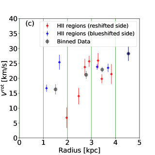
Figure 8: The rotation velocities from the line of sight velocities based on the Hi ’s ring parameters. These velocities are further rebinned with a radial bin of 1.0 kpc.

3.1.3 The contribution to the rotation curve from the gravity of gas

The radial profile of the gas mass surface density derived from the tilted-ring modeling is shown in Figure 2 (c). We used this profile to estimate the gas rotation curve using the ROTMOD task (Begeman, 1989) in the GIPSY package. The gas mass has been corrected for helium by multiplying it by a factor of 1.36. The vertical distribution of the gas disk is assumed to be “SECH-SQUARED” with a scale height of 0.1 kpc. By varying the gas mass surface density with its error, we used the Monte-Carlo method to estimate the uncertainty of the rotation curve. We then varied the scale height from 0.02 kpc to 0.5 kpc to quantify the effect of the scale-height uncertainty on the rotation curve. The two types of errors were summed quadratically to get the final error.

3.1.4 The contribution to the rotation curve from the gravity of stars

To estimate the stellar mass distribution, we first derived the radial profile of the 3.6 $\mu$m surface brightness at a bin width of 3$\arcsec$, half of the resolution FWHM. The ellipse parameters derived by the above Hi  dynamical modeling were used, for which the inclination angle and the position angle were interpolated. We then converted this brightness into the stellar mass profile using $\Upsilon_{3.6{\mu}m}$=0.6 $M_{\odot}/L_{\odot,3.6{\mu}m}$ with a Kroupa stellar initial mass function (see below), as shown in Figure 4 (b). To extend the profile to 10 kpc, an exponential disk was fitted to the part outside a radius of 4 kpc.

To measure the stellar contribution to the rotation curve, we use the ROTMOD task (Begeman, 1989) in GIPSY, where the vertical distribution was assumed to be “SECH-SQUARED” with a scale height of 0.2 kpc. The errors of the stellar mass surface density are dominated by the subtraction of the sky background and its effects on the rotation curve are simulated with the Monte Carlo method. We also varied the scale height from 0.01 kpc to 0.5 kpc to obtain the uncertainty due to the scale height. The above two errors were quadratically added to represent the final error of the stellar rotation curve.

3.2 The models of dark matter halo

The models of cuspy dark matter halo are motivated by numerical simulations of dark matter, including a Navarro-Frenk-White (NFW) model (Navarro et al., 1997) and an Einasto model (Einasto, 1965). The models of cored dark matter halo are observatinally motivated, including the pseudo-isothermal (ISO) model (Begeman et al., 1991) and Burkert model (Burkert, 1995).

1) A NFW halo model (Navarro et al., 1997) has a density profile of

$$\rho_{\rm NFW}(R)=\frac{{\rho_{c}}{\delta_{\rm char}}}{(R/R_{S})(1+R/R_{S})^{2}},$$ (4)

where $\rho_{c}$=3$H^{2}$/(8$\pi$G) is the present critical density, $\delta_{\rm char}$ is dimensionless density contrast and $R_{S}$ is the scale radius. $R_{S}$ is related to $R_{200}$ through the concentration $c$=$R_{200}$/$R_{S}$, where $R_{200}$ is the radius within which the halo average density is 200 times the present critical density. $\delta_{\rm char}=\frac{200c^{3}g}{3}$ with $g=\frac{1}{{\rm ln}(1+c)-c/(1+c)}$. The halo mass with $R_{200}$ is $M_{200}=\frac{100H^{2}R_{200}^{3}}{G}$. The inner density profile of the NFW model shows a cusp with $\rho$ $\propto$ $R^{-1}$. The corresponding rotation velocity of the NFW model is

$$V_{\rm NFW}(R)=V_{\rm 200}\sqrt{\frac{{\rm ln}(1+cx)-cx/(1+cx)}{x\left[{\rm ln}(1+c)-c/(1+c)\right]}},$$ (5)

where $V_{\rm 200}$ is the circular velocity at $R_{200}$ with $V_{\rm 200}$=$R_{\rm 200}h$, and $x$=$R$/$R_{200}$.

2) A pseudo-isothermal halo model (Begeman et al., 1991) is observationally motivated to describe the presence of a central core:

$$\rho_{\rm ISO}(R)=\frac{\rho_{0}}{1+(R/R_{C})^{2}},$$ (6)

where $\rho_{0}$ is the central density and $R_{C}$ is the core radius of the halo. The rotation velocity is

$$\begin{multlined}V_{\rm ISO}(R)=\sqrt{4{\pi}G\rho_{0}R_{C}^{2}\left[1-\frac{R_{C}}{R}{\rm arctan}(\frac{R}{R_{C}})\right]}\\ =V_{\rm norm}\sqrt{(\frac{R_{C}}{R_{1}})^{2}\left[1-\frac{R_{C}}{R}{\rm arctan}(\frac{R}{R_{C}})\right]},\end{multlined}V_{\rm ISO}(R)=\sqrt{4{\pi}G\rho_{0}R_{C}^{2}\left[1-\frac{R_{C}}{R}{\rm arctan}(\frac{R}{R_{C}})\right]}\\ =V_{\rm norm}\sqrt{(\frac{R_{C}}{R_{1}})^{2}\left[1-\frac{R_{C}}{R}{\rm arctan}(\frac{R}{R_{C}})\right]},$$ (7)

where $V_{\rm norm}$ = $R_{1}\sqrt{4{\pi}G\rho_{0}}$ and $R_{1}$=1 kpc.

3) The Burkert density profile (Burkert, 1995) is described by

$$\rho_{\rm Bk}(R)=\frac{\rho_{0}R_{C}^{3}}{(R+R_{C})(R^{2}+R_{C}^{2})},$$ (8)

where $\rho_{0}$ and $R_{C}$ are the central core density and core radius, respectively.

The corresponding circular velocity is given by

$$V_{\rm Bk}(R)=V_{C}\sqrt{\frac{2\,{\rm ln}(1+x)+{\rm ln}(1+x^{2})-2\,{\rm arctan}(x)}{x\left[3\,{\rm ln}(2)-2\,{\rm arctan}(1)\right]}},$$ (9)

where $x$=$R/R_{c}$ and $V_{C}$ is the circular velocity at the core radius.

4) With the rotation curve of a dark matter halo, the density profile of the halo can be derived through (de Blok et al., 2001):

$$\rho(R)=\frac{1}{4{\pi}G}\left[\frac{2V}{R}\frac{{\partial}V}{{\partial}R}+(\frac{V}{R})^{2}\right]$$ (10)

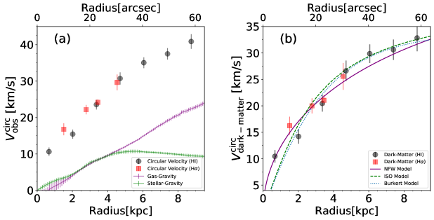
Figure 9: The rotation curves of AGC 242019. a, The observed rotation curves from the Hi  data (black circles) and the H$\alpha$ data (red rectangles), along with the rotation curves due to the gas and stellar gravity contributions. b, The derived rotation curve of dark matter. Different curves indicate the best-fitted NFW, ISO and Burkert models to the HI only rotation curve.

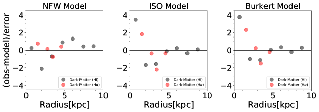
Figure 10: The residuals of the fitting to the dark-matter rotation curve for three models.

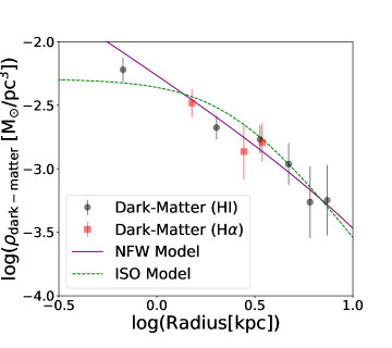
Figure 11: The density profile of dark matter of AGC 242019. Two curves represent the best-fitted NFW and ISO models to the HI rotation curve.

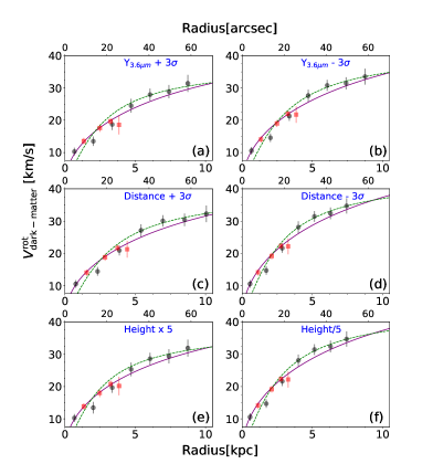
Figure 12: The rotation curves of dark matter by varying different parameters. a-b, The results with the mass-to-light ratio in 3.6 $\mu$m varying by $\pm$3-$\sigma$. c-d, The results with the distance varying by $\pm$3-$\sigma$. e-f, The results with the scale height of the Hi  gas disk varying by a factor of five.

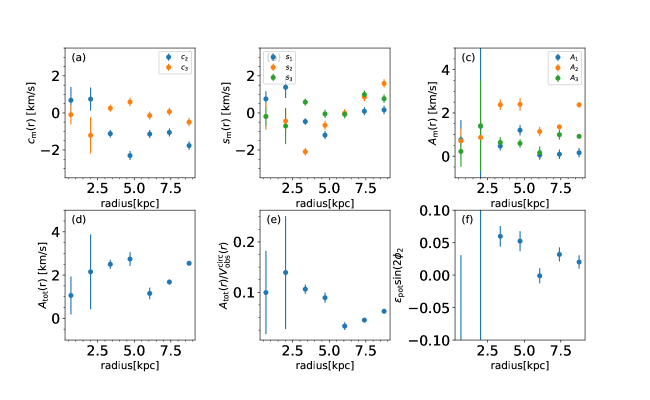
Figure 13: The results of harmonic expansion of non-circular motions. a, The individual $c$ component up to the harmonic order of 3. b, The individual $s$ component up to the harmonic order of 3. c, The amplitude of each harmonic order. d, The total harmonic amplitude. e, The ratio of the total harmonic amplitude to the circular velocity. f, The elongation of the potential as described by ${\epsilon}_{\rm pot}{\rm sin}2\phi_{2}$.

3.3 Priors and set-ups of the rotation curve modeling

Table 3: The priors for the dark-matter modeling

Parameters	Bounded Normal ($\mu$, $\sigma$)
NFW model
$R_{\rm 200}$	(75, 150) kpc
$R_{\rm S}$	(7.5, 15) kpc
ISO model
$V_{\rm norm}$	(25, 50) km s-1
$R_{\rm C}$	(2, 4) kpc
Burkert model
$V_{\rm C}$	(35, 70) km s-1
$R_{\rm C}$	(2, 4) kpc

We fitted the above three dark-matter models to the rotation curve of dark matter through Bayesian inference with the Python code PyMC3 (Salvatier et al., 2016). We adopted the No-U-Turn Sampler (NUTS) with 5000 samples, 2000 tune, 4 chains and target_accept=0.99.

As listed in Table 3, the prior of each parameter of a dark-matter model is described with a bounded normal distribution, whose lower-limit bound is set to be zero. The mean of the distribution is set with some prior knowledge as detailed below, and the standard deviation is set to be twice the mean.

The prior $R_{200}$ of the NFW model is set to have a mean of 75 kpc, corresponding to a halo mass of 5$\times$10¹⁰ $M_{\odot}$ as expected by the stellar mass vs. halo mass relationship given our stellar mass of (1.37$\pm$0.05)$\times$10⁸ M_⊙  (Santos-Santos et al., 2016). At this halo mass, the halo concentration is about 10 in simulations (Macciò et al., 2007), giving the mean prior $R_{S}$ of 7.5 kpc.

Since the core radius of a cored dark-matter halo is on a kpc scale (Oh et al., 2015), the mean prior $R_{\rm C}$ of the ISO model is set to be 2 kpc. The mean prior $V_{\rm norm}$ of the ISO model is thus set to be 25 km s^-1, so that the galaxy is on the baryonic Tully-Fisher relationship (Mancera Piña et al., 2020) given its stellar mass of (1.37$\pm$0.05)$\times$10⁸ M_⊙  and a HI mass of (8.51$\pm$0.36)$\times$10⁸ M_⊙ . Similarly, the mean prior $R_{\rm C}$ of the Burkert model is set to be 2 kpc, and the mean prior $V_{\rm C}$ of the model is set to be 35 km s^-1.

The fitting is convergent. By exploring the full posterior distribution, the best-fitted parameter is given as the mean of the distribution, and the error is given by the standard deviation, as well as the 3% and 97% Highest Posterior Density (HPD). The percentage of small Pareto shape diagnostic values ($k$ $<$ 0.7) is also listed. A larger diagnostic value indicates that the model is mis-specified.

4 Results

4.1 The rotation curve of dark matter

Figure 9 (a) shows the observed rotation curve of AGC 242019. The Hi  measurements cover a radial extent of 9 kpc while the H$\alpha$  data cover the central 5 kpc in radius. Two datasets are overall consistent with each other in the overlap region. The rotation curve rises all the way up to the last measurable radius.

Figure 9 (b) shows the rotation curve of dark matter after quadratically subtracting the gas and stellar gravity contributions. The sampling of the Hi  curve is at the beam size, while the H$\alpha$ curve has a radial bin of 1.0 kpc. As shown in the figure, the H$\alpha$  curve is overall well consistent with the Hi  curve over the spatial extent where both dataset cover. As mentioned before, since the H$\alpha$ emission is sporadic and the errors of the H$\alpha$  rotation curve are only based on the detected regions, its rotation curve is only used for the sanity check of the Hi  curve. We fitted the Hi  curve with two spherical halo models, namely, the NFW model (Equation 5, Navarro et al., 1997) and the ISO model (Equation 7, Begeman et al., 1991), through the Python code PyMC3 (Salvatier et al., 2016) to represent the cuspy and cored profiles, respectively. The ISO model is too steep at the inner radii, whereas the NFW model matches the observed data in the overall fitting, which is also illustrated by the fitting residuals as shown in Figure 10. To quantitatively discriminate the two models, we performed a leave-one-out (LOO) predictive check (Vehtari et al., 2015). We found that the estimated effective number of parameters ($p_{\rm loo}$=1.6) of the NFW model is smaller than the real number of free parameters, i.e., two, while that of the ISO model has $p_{\rm loo}$=6.3, significantly larger than two (see Table 4). This quantitatively indicates that the NFW model is valid, while the ISO model is ruled out. The corresponding difference in the reduced $\chi^{2}$ is 1.9 for d.o.f.=5, equivalent to a Gaussian significance of 3.0-$\sigma$. As listed in Table 4, some Pareto diagnostic value $k$ of the ISO model is larger than 0.7, further indicating that the model is mis-specified. We also run the fitting by including the H$\alpha$ , and obtained similar difference in $p_{\rm loo}$ values and $\Delta(\chi^{2}$/d.o.f.)=2.8 for d.o.f.=9 between the two models, equivalent to a Gaussian significance of 5.0-$\sigma$.

The Burkert model is another observationally-motivated formula to describe a cored dark matter halo (Equation 9, Burkert, 1995). Its density profile is flat toward the center, which is like the ISO model, but has a power law index of -3.0 toward infinity, which is like the NFW model. As shown in Figure 9 (b), the Burkert model gives a bad fitting too, with $p_{\rm loo}$=4.4, much larger than (1.6) that of the NFW model.

The best-fitted NFW model has a halo scale radius of $\sim$33 kpc. Such a large cusp is well spatially resolved given that its size relative to the Hi  beam is 24. This suggests that the presence of the cusp is not an artifact caused by a limited spatial resolution (de Blok et al., 2001; Oh et al., 2015). The dark-matter halo has a mass of (3.5$\pm$1.2)$\times$10¹⁰ M_⊙  within $R_{200}$, the radius at which the average halo density is 200 times the average cosmic density. Due to the fact that the rotation curve does not reach the flat part, the constraints on the $R_{200}$ (or $M_{\rm halo}$) and $R_{\rm S}$ do not reach a small error. But a small halo concentration of only 2.0$\pm$0.36  is conclusive. This is much smaller than the median concentration of 15 at the same halo mass in the local Universe (Macciò et al., 2007). The implication of this small concentration on the formation of the galaxy is discussed in § 5.3.

To constrain the innermost density slope $\alpha_{\rm innermost}$ of the dark matter halo, we derived the density profile of dark matter from the rotation curve (de Blok et al., 2001) as shown in Figure 11. Following de Blok et al. (2001) and Oh et al. (2015), we measured $\alpha_{\rm innermost}$ by carrying out the least-square fitting to the density profile within the break radius, and defined the error of $\alpha_{\rm innermost}$ as the difference between the result including the first data-point outside the break radius and the result including only data-points within the break radius. Here the break radius is the radius where the density profile shows a maximum change in the slope. If adopting the core radius of the best-fitted ISO model as the break radius, $\alpha_{\rm innermost}$=-($0.96\pm 0.12$). If adopting the scale radius of the best-fitted NFW model as the radius, $\alpha_{\rm innermost}$=-(0.90$\pm$0.08). Here the error is given by the least square fitting since the scale radius of the NFW model is larger than the last ring. Two measurements indicates a statistical significance of about 10-$\sigma$ that the dark matter halo of AGC 242019 is cuspy down to a radius of 0.67 kpc .

Table 4: The fitting result of NFW and ISO models to the dark-matter rotation curve with PyMC3

Rotation Curves	NFW model						ISO model
	$R_{200}$	$R_{s}$	$p_{\rm LOO}$	$k^{\ast}$ ($<$0.7)	$\chi^{2}$/d.o.f.¶		$V_{\rm norm}$	$R_{\rm C}$	$p_{\rm LOO}$	$k^{\ast}$ ($<$0.7)	$\chi^{2}$/d.o.f.¶
	(kpc)	(kpc)					(km s-1)	(kpc)
HI (fiducial)	65.0$\pm$7.4	33.3$\pm$9.1	1.6	100%	1.60		16.7$\pm$1.9	2.5$\pm$0.5	6.3	86%	3.51
HI+H$\alpha$ (fiducial)	64.6$\pm$7.1	33.1$\pm$8.7	1.2	100%	1.90		17.1$\pm$1.7	2.2$\pm$0.4	5.8	100%	4.74
HI ($\Upsilon_{3.6{\mu}m}$+3$\sigma$)	59.5$\pm$7.2	31.5$\pm$9.3	1.4	100%	1.32		16.3$\pm$2.3	2.3$\pm$0.5	7.3	86%	3.55
HI ($\Upsilon_{3.6{\mu}m}$-3$\sigma$)	67.2$\pm$7.7	33.6$\pm$9.1	1.8	100%	1.82		16.9$\pm$1.8	2.5$\pm$0.4	6.5	86%	3.50
HI (Distance+3$\sigma$)	62.1$\pm$6.7	33.9$\pm$9.2	1.7	100%	1.66		15.2$\pm$1.8	2.6$\pm$0.5	7.1	86%	3.46
HI (Distance-3$\sigma$)	73.8$\pm$8.5	33.9$\pm$8.9	1.9	100%	1.97		19.5$\pm$2.0	2.3$\pm$0.4	6.2	86%	3.55
HI (5$\times$Height)	60.7$\pm$7.4	30.6$\pm$9.0	1.0	100%	1.14		17.5$\pm$2.6	2.2$\pm$0.5	6.7	86%	3.29
HI (Height/5)	61.6$\pm$7.4	31.4$\pm$9.1	1.1	100%	1.34		17.6$\pm$3.0	2.2$\pm$0.6	9.9	86%	3.93

Table 5: The fitting result of the Burkert model to the HI’s curve of dark matter

$V_{C}$ [km/s]	$R_{C}$ [kpc]	$p_{\rm LOO}$	$k^{\ast}$ ($<$0.7)	$\chi^{2}$/d.o.f.¶
25.7$\pm$1.9	4.4$\pm$0.7	4.4	86%	3.34

4.2 The systematic uncertainties of the dark-matter rotation curve

The identification of a cuspy profile in AGC 242019 is robust against systematic uncertainties from several aspects.

(1) Position and inclination angles: Since these two angles have been set as free parameters during the fitting, their uncertainties have already been included in the derived rotation curve. For comparison, we further estimated the photometric position and inclination angles based on the $r$-band image. The galaxy in the $r$-band is somewhat asymmetric with clumpy features, but outside the radius of 8^′′, the position angle and inclination angles converge to (2$\pm$2)^∘ and (67$\pm$3)^∘, respectively. These results are consistent with the values derived from the dynamic fitting of the Hi  data, as shown in Figure 5 and listed in Table 2.

(2) Mass-to-light ratio in 3.6 $\mu$m: The rotation velocity due to stellar gravity is proportional to the square root of the stellar mass-to-light ratio. The overall stellar contribution to the observed rotation curve is small, so our result is not sensitive to the mass-to-light ratio $\Upsilon_{3.6{\mu}m}$, as is detailed here. The mass-to-light ratio in a broad band is obtained by fitting a synthetic spectrum to the observed spectrum or a broad-band spectral energy distribution. The uncertainties of the stellar population synthesis model, the star formation history, the dust extinction, the metallicity and the initial mass function all result in the variation of the derived mass-to-light ratio.

With the measured stellar mass and star formation rate of AGC 242019, we assumed a low metallicity with [Fe/H]=-1 and suppressed asymptotic giant branch (AGB) stars, as seen in some low surface brightness dwarfs (Schombert et al., 2019), to derive the $\Upsilon_{3.6{\mu}m}$ of our target to be 0.6 (Schombert et al., 2019). The preceding assumption about AGB stars causes the mass-to-light ratio to be $\sim$ 30% larger than that in normal galaxies. $\Upsilon_{3.6{\mu}m}$ is also color dependent (Bell et al., 2003; Zibetti et al., 2009; Jarrett et al., 2013; Meidt et al., 2014; Shi et al., 2018; Schombert et al., 2019; Telford et al., 2020). As the object is not detected in 4.5 $\mu$m, we used the radial variation in $g-r$ color with a median of 0.3 and standard deviation of 0.03. Converting to $B-V$ = 0.98*($g-r$) + 0.22 (Jester et al., 2005), the variation in $\Upsilon_{3.6{\mu}m}$ is expected to have a standard radial deviation as small as 0.02 dex (Schombert et al., 2019), and thus, its effects on the rotation curve of dark matter are negligible.

The systematic uncertainties due to the difference in star formation histories, initial mass functions and stellar population models among different studies are much larger even at a fixed color (Bell et al., 2003; Zibetti et al., 2009; Jarrett et al., 2013; Meidt et al., 2014; Schombert et al., 2019; Telford et al., 2020). As a result, we adopted 0.1 dex as the 1-$\sigma$ error to encompass the results in different studies. We then varied $\Upsilon_{3.6{\mu}m}$ by $\pm$3$\sigma$ to investigate its effect on the rotation curve of dark matter. As listed in Table 4 and shown in Figure 12, the cusp-like NFW model is a more reasonable model than the core-like ISO model for both $\Upsilon_{3.6{\mu}m}$ values.

(3) Distance: The velocities due to baryonic gravity vary with the square root of the distance, while the observed rotation curve is independent of the distance. As the object is an isolated galaxy with no close-by companion that is brighter than $m_{r}$ $=$ 17.7 (or $M_{r}$ $=$ -14.8) within 500 kpc and 1000 km s^-1  in the Sloan Digital Sky Survey, the error in the distance is dominated by the uncertainty of the Hubble constant and the peculiar velocity. The heliocentric velocity is 2237 km s^-1  after correcting for the Virgo, Great Attractor and Shapley supercluster (Mould et al., 2000). We estimated the residual error to be 100 km/s, which corresponds to an infalling velocity toward an imaginary dark matter halo with 10¹¹ $M_{\odot}$ at a separation of 50 kpc. By adopting a local Hubble constant of 73 km s^-1  with 2.5% uncertainty (Riess et al., 2016), the distance thus has a 1-$\sigma$ uncertainty of 5%. We varied this distance by $\pm$3$\sigma$ to investigate its effect on the dark-matter rotation curve. As listed in Table 4 and shown in Figure 12, the cusp-like NFW model is again advocated against the core-like ISO model for both distances.

(4) The scale height of the gas disk: For a thick disk, emissions from adjacent rings are projected to be in the same pixels, which causes a beam smearing and affects the measurements of the inclination and position angles. By increasing and decreasing the scale height by a factor of five to 500 pc and 20 pc, respectively, the NFW model is still much better than the ISO model, as shown in Figure 12 and Table 4.

(5) The noncircular motion: As shown in Figure 6, the median amplitude of the residual velocity obtained by ^3DBarolo fitting is small, i.e., $\sim$2 km s^-1. During the fitting, the line-of-sight velocities are assumed to be entirely circular motions, while noncircular motions cause the real circular velocity to be underestimated. To quantify the amplitude of noncircular motions, we carried out harmonic decomposition with the GIPSY task RESWRI (Begeman, 1989). As detailed in previous studies (Schoenmakers et al., 1997; Trachternach et al., 2008), the line-of-sight velocity of each ring can be decomposed into

$$v_{\rm los}(r)=v_{\rm sys}(r)+\Sigma_{m=1}^{N}(c_{m}(r){\rm cos}m\psi+s_{m}(r){\rm sin}m\psi),$$ (11)

where $r$ is the radial distance of each ring from the dynamical center, $v_{\rm sys}(r)$ is the system velocity, $\psi$ is the azimuthal angle in the plane of the disk. $v_{\rm los}(r)=v_{\rm sys}(r)+c_{1}(r){\rm cos}\psi$ corresponds to a pure circular motion scenario. In this study, we expanded the velocity up to $m$=3, as has been adopted in other studies (Schoenmakers et al., 1997; Trachternach et al., 2008).

To run RESWRI, we used the 2-D velocity field produced by ^3DBarolo as the input, fixed the dynamical center and system velocity to those determined by ^3DBarolo, and set the rotation velocity, inclination angle and position angle of each ring as free parameters. With the derived $c_{m}$ and $s_{m}$, the amplitude of each noncircular harmonic component with $m>$1 is defined as

$$A_{m}(r)=\sqrt{c_{m}^{2}(r)+s_{m}^{2}(r)}$$ (12)

and for $m$=1 where $c_{1}$ is the circular motion,

$$A_{1}(r)=\sqrt{s_{1}^{2}(r)}.$$ (13)

The total amplitude of noncircular motion is given by

$$A_{\rm tot}(r)=\sqrt{s_{1}^{2}(r)+c_{2}^{2}(r)+s_{2}^{2}(r)+c_{3}^{2}(r)+s_{3}^{2}(r)}.$$ (14)

The measured harmonic component can be used to quantify the elongation of the potential $\epsilon_{\rm pot}$ at each radius as follows:

$${\epsilon}_{\rm pot}{\rm sin}2\phi_{2}=(s_{3}-s_{1})\frac{1+2q^{2}+5q^{4}}{c_{1}(1-q^{4})},$$ (15)

where $\phi_{2}$ is an unknown angle between the minor axis of the elongated ring and the observer in the plane of the ring and $q$ = cos $i$, with $i$ being the inclination angle of the disk.

Figure 13 shows the result of the harmonic decomposition. As shown in Figure 13 (a), the radial $c_{m}$ fluctuates around 0 km/s with amplitudes $\lesssim$ 2 km/s. The radial $s_{m}$ shows similar behaviors with amplitude $\lesssim$ 2 km/s. As a result, the $A_{m}$ of each harmonic component is in general $\lesssim$ 2 km/s. Figure 13 (d) shows that the total amplitude $A_{\rm tot}$ is only about 2 km/s. As shown in Figure 13 (c), all the amplitudes are small fractions of the circular velocities at the corresponding radii that are $<$ 15%.

Compared to other galaxies with similar absolute magnitudes (Trachternach et al., 2008), AGC 242019 is indeed a galaxy without stronger noncircular motions. Compared to simulated galaxies where noncircular motions result in noticeable underestimations of circular velocities (Oman et al., 2019), the noncircular amplitude of $\sim$ 2 km/s in AGC 242019 is much less than the simulated values of 20-30 km/s. Therefore, we expect that the noncircular motion of AGC 242019 should not affect the derived rotation curve of dark matter. Finally, the derived ${\epsilon}_{\rm pot}{\rm sin}2\phi_{2}$, as shown in Figure 13 (f), suggests a spherical gravitational potential.

(6) The triaxiality of a dark matter halo: In this study a spherical dark matter halo is assumed, while a halo has been found to be moderately triaxial in numerical simulations (Jing & Suto, 2002; Bailin & Steinmetz, 2005). However, a typical triaxial mass distribution results in only a small deviation in the density from the spherical assumption. Within the scale radius of the halo, the difference is only 10-20%, which is much smaller than the required variation of a factor of 3 to decrease the inner slope by 0.5 (Knebe & Wießner, 2006). Numerical modeling of the rotation curve further suggests that the halo triaxiality cannot significantly change the shape of the curve to make an intrinsic cusp to be a core (or vice versa) in the observed data (Kuzio de Naray et al., 2009; Kuzio de Naray & Kaufmann, 2011).

(7) Beam smearing: ^3DBarolo takes the beam smearing into account in the tilted-ring fitting (Di Teodoro & Fraternali, 2015). ^3DBarolo first builds a gas disk in three spatial dimensions and three velocity dimensions, and then convolves this artificial disk to the observed spatial resolution for comparison with the observed 3-D datacube to derive the best-fitting parameters. It has been shown that ^3DBarolo is able to recover the rotation curve even at a low spatial resolution, i.e., two resolution elements over the semimajor axis (Di Teodoro & Fraternali, 2015). The semimajor axis of AGC 242019 is resolved into $\sim$ 7 beams in the Hi  map. In addition, the H$\alpha$ map has a rebinned spatial resolution (4^′′ in diameter) that is two times higher than the Hi  map. Although our H$\alpha$ clumps are mainly distributed along the major axis with a narrower spatial extent, the overall shape of the H$\alpha$-derived curve is consistent with the Hi  curve, demonstrating that the beam smearing effect on the Hi ’s rotation curve has been largely removed by ^3DBarolo (Di Teodoro & Fraternali, 2015).

(8) The contributions from molecular gas and ionized gas: The very low surface density of AGC 242019 results in a low mid-plane pressure with a $P_{\rm ext}/k$ $\lesssim$ 10³ cm^-3 K, which gives a molecular-to-atomic gas ratio of $\lesssim$ 5% (see their Figure 3 and Equation 12 in studies of nearby galaxies (Blitz & Rosolowsky, 2006; Leroy et al., 2008)). We also checked that the atomic gas alone is sufficient to place the galaxy in the extended Schmidt law (Shi et al., 2011, 2018), consistent with a negligible fraction of molecular gas.

The ionized gas mass can be estimated from the H$\alpha$ luminosity by $M_{\rm HII}=m_{\rm p}\frac{L_{Ha}}{3.56{\times}10^{-25}N_{e}}$ (Osterbrock & Ferland, 2006), where $m_{\rm p}$ is the proton mass, $L_{Ha}$ is the H$\alpha$ luminosity in erg/s, and $N_{e}$ is the electron volume density in cm^-3. By assuming a low $N_{e}$ of 100 cm^-3, we found that, even at the peak spaxel as shown in Figure 4 (c), an ionized gas mass surface density of 0.025 $M_{\odot}$/pc² is too small to affect the derived rotation curve of dark matter.

5 Discussions

Through measurements of the dynamics of atomic and ionized gas, we demonstrate that the dark matter halo of AGC 242019 can be well fitted by the cuspy profile as described the NFW model, while excluding cored models including ISO and Burkert ones. We here discuss its constraints on the alternatives of standard cold dark matter, implications for the role of feedback and implications for formation of UDGs.

5.1 Implications for the alternatives of standard cold dark matter

5.1.1 Fuzzy cold dark matter

Through numerical simulations, a halo of fuzzy cold dark matter is found to be composed of a soliton core superposed on an extended halo (Hu et al., 2000; Schive et al., 2014). The latter can be represented by the NFW model, while the former can be approximately described by:

$$\rho_{c}(r)\approx\frac{1.9(m_{\psi}/10^{-23}{\rm eV})^{-2}(R_{c}/{\rm kpc})^{-4}}{\left[1+9.1\times 10^{-2}(r/R_{c})^{2}\right]^{8}}{\rm M_{\odot}pc^{-3}},$$ (16)

where $m_{\psi}$ is the particle mass and $R_{c}$ is the core radius. The soliton core is linked to the total halo through the core-halo relationship (Schive et al., 2014), which gives

$$R_{c}=1.6(m_{\psi}/10^{-22}{\rm eV})^{-1}(M_{\rm h}/10^{9}M_{\odot})^{-1/3}{\rm kpc}.$$ (17)

As shown in Figure 9 (b), a NFW model fits the density profile of AGC 242019 very well, which shows negligible residual density for the soliton core to account for. As a result, the possible contribution to the dark-matter density from the soliton core should not exceed the observed error at all radii, which can be used to constrain the $m_{\psi}$. For each radius, we estimated the density of the soliton core as a function of the particle mass $m_{\psi}$ with the best-fitted $M_{\rm h}$=(3.5$\pm$1.2)$\times$10¹⁰ M_⊙  through the above two equations. It is found that the measurements at the innermost two radii give the strongest constraints on $m_{\psi}$. The 3-$\sigma$ observed errors at two radii constrain the $m_{\psi}$ range to be $<$ 0.06$\times$10^-22 eV  or $>$ 2.7$\times$10^-22 eV . Compared to the constraint from Ly$\alpha$ forest in which $m_{\psi}$ $<$ 1.0$\times$10^-22 eV or $m_{\psi}$ $>$ 23$\times$10^-22 eV, the dynamics of AGC 242019 gives a factor of about 20 times smaller constraint on the upper-bound of the lower range. As shown in Figure 14 (a), if adopting the 3% HPD halo mass of 1.5$\times$10¹⁰ M_⊙ , $m_{\psi}$ $<$ 0.11$\times$10^-22 eV  or $m_{\psi}$ $>$ 3.3$\times$10^-22 eV  whose upper-bound of the lower range is still 10 times lower than the constraint by the Ly$\alpha$ forest. If somehow our error is underestimated by a factor of 2, the upperbound of the lower range only increases by a factor of $\sim$ 1.6, and the lowerbound of the upper range decreases by a factor of $\sim$ 1.2. Therefore, the constraint by AGC 242019, along with the one from the Ly$\alpha$ forest, is inconsistent with the typical $m_{\psi}$ of $\sim$ 10^-22 eV that is required to explain the dynamics of other galaxies with cored dark-matter halos (Hu et al., 2000; Schive et al., 2014). It is thus found that there is no $m_{\psi}$ value that can reconcile all the observational facts.

5.1.2 Self-interacting Dark Matter

Self-interacting dark matter transmit the kinetic energy from the outer part inward to form a constant density core. For the interaction to be efficient, the scattering rate per particle should be important, that is at least once over the galaxy age (Spergel & Steinhardt, 2000; Rocha et al., 2013; Tulin & Yu, 2018):

$${\Gamma}(r)t_{\rm age}{\approx}\rho(r)(\sigma/m)v_{\rm rms}(r)t_{\rm age}{\sim}1,$$ (18)

where is ${\Gamma}(r)$ is the scattering rate per particle, $\rho(r)$ is dark matter density at a radius of $r$, $\sigma/m$ is the cross section per particle mass and $v_{\rm rms}$ is the relative velocity of dark matter particles. The above equation can be re-written as:

$$\frac{\sigma/m}{\rm 1\;cm^{2}/g}{\approx}(\frac{\rm 9.2\;Gyr}{t_{\rm age}})(\frac{\rm 0.01\;M_{\odot}/pc^{3}}{\rho(r)})(\frac{\rm 50\;km/s}{v_{\rm rms}}).$$ (19)

For AGC 242019, the NFW model fits the rotation curve well down to the innermost radius. This sets the upperlimit to the radius of a possible density core and the lowerlimit to the above $\rho(r)$ if dark matter is self-interacting in AGC 242019. If the halo forms around $z$=2, we got $t_{\rm age}$ = 10 Gyr. The $v_{\rm rms}$ is set to be the virial velocity at the virial radius, which is 47 km s^-1 . we have $\sigma$/m $<$ 1.63 cm²/g  for AGC 242019.

As shown in Figure 14 (b), existing studies prefer somewhat larger $\sigma/m$ on galaxy scales (Elbert et al., 2015; Kaplinghat et al., 2016; Zavala et al., 2013) and smaller values on cluster scales (Kahlhoefer et al., 2015; Randall et al., 2008; Harvey et al., 2015; Kaplinghat et al., 2016). Such a velocity dependence of the cross section seems to reconcile results over different scales (Kaplinghat et al., 2016). However, the cuspy dark matter halo of AGC 242019 may challenge this simple picture, whose upperlimit to $\sigma/m$ is somewhat in tension with the lowerbound of the $\sigma/m$ range as required by cored halos of other dwarf galaxies.

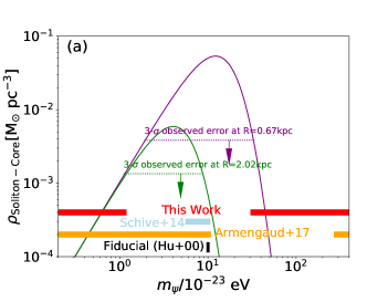
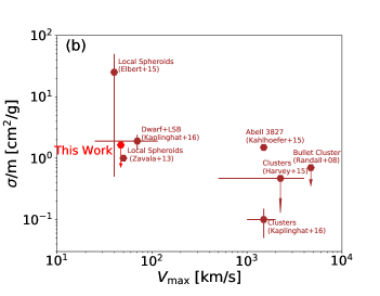
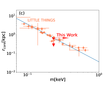
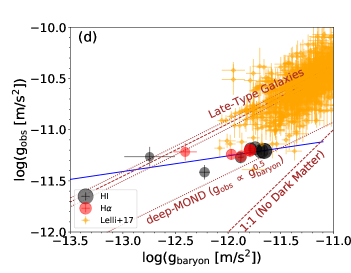
Figure 14: Test of the alternatives of standard cold dark matter with AGC 242019. a, The test of the fuzzy dark matter. Two curves represent the soliton core mass density as a function of the dark matter particle mass at the innermost and second innermost rings, respectively. The dotted lines are the observed 3-$\sigma$ errors at the corresponding two radii. Color bars are the constraint of the particle mass by different studies (see text). b, The test of the self-interacting dark matter. Brown symbols are the constraints in the literature. The density of the innermost ring of AGC 242019 results in the upperlimit of the cross section of self-interacting dark matter. c, The test of warm dark matter. The radius of the innermost ring of AGC 242019 marks the lowerbound of the particle mass of warm dark matter. d, The test of MOND through the relationship between the observed radial acceleration and the baryonic radial acceleration. The black/red symbols are the results of AGC 242019, where a larger symbol size corresponds to the ring with a larger radius. The blue solid line is the best linear fit to the observations. Lines labeled with “Late-Type Galaxies” and orange symbols are the best-fitted line plus its scatter and individual late-type galaxies in Lelli et al. (2017). The dotted line labeled with “deep-MOND” is the MOND prediction in the low acceleration regime with a slope of 0.5. The dashed line labeled with “No Dark Matter” is the no dark matter line.

5.1.3 Warm Dark Matter

In warm dark matter, the density core has a size that can be approximately by Hogan & Dalcanton (2000); Macciò et al. (2012)

$$r^{2}_{\rm core}=\frac{\sqrt{3}}{4\pi GQ_{\rm max}}\frac{1}{<v_{\rm rms}^{2}>^{0.5}},$$ (20)

where $v_{\rm rms}$ is the velocity dispersion (i.e. the mass) of the halo. $Q_{\rm max}$ is the maximum phase density as given by

$$Q_{\rm max}=1.64\times 10^{-3}(\frac{\rho_{\rm L}}{\rho_{\rm cr}})(\frac{m}{\rm keV})^{4}\frac{\rm M_{\odot}\;pc^{-3}}{\rm(km\;s^{-1})^{3}},$$ (21)

where $m$ is the mass of warm dark matter, $\frac{\rho_{\rm L}}{\rho_{\rm cr}}$ is the local density relative to the critical density.

$$\frac{m}{\rm keV}=0.37\frac{1}{(\rho_{\rm L}/\rho_{\rm cr})^{0.25}}*(\frac{\rm kpc}{r_{\rm core}})^{0.5}(\frac{\rm km/s}{<v_{\rm rms}^{2}>^{0.5}})^{0.25}.$$ (22)

As shown in Figure 14 (c), the innermost radius of the cuspy halo of AGC 242019 leads to $m$ $>$ 0.23 keV . The figure also includes the constraints from the LITTLE THINGS galaxies (Oh et al., 2015) that are derived from the core radius and the velocity at the outermost measurable radius listed in their Table 2. It seems that there is no consistent mass range that can explain all observational facts. Warm dark matter is known to have a “catch-22” problem: the requirement for the particle mass to solve the cuspy-core problem will result in no formation of small galaxies at the first place. Our discovery of a cuspy dark matter halo in AGC 242019 will further challenge the warm dark matter scenario, such that, even on kpc scales, the required particle mass cannot reconcile with the constraint that accounts for cored halos in some other dwarf galaxies.

5.1.4 The modified Newtonian dynamics

Unlike massive disk galaxies whose baryonic disk surface density rises exponentially toward their galactic centers, AGC 242019 shows a much flatter profile with a density deficit in the central region. Such a distinct spatial offset between the baryonic matter and the dynamical mass leads to an increasing baryonic matter relative to dark matter at larger radii, in contrast to galaxies in general. This can be quantified by the logarithmic relationship between the observed radial acceleration and the baryonic radial acceleration as shown in Figure 14 (d). From the inner (smaller symbols) to larger radii (larger symbols), the data are more closer to no dark matter line, demonstrating the increasing baryonic matter relative to the dark matter at larger radii.

The modified Newtonian dynamics (MOND) paradigm (Milgrom, 1983) has been proposed as an alternative to dark matter theory for interpreting dynamical features. However, MOND cannot explain the dynamics of AGC 242019 as specified by the radial acceleration relationship shown in Figure 14 (d). The relationship has a slope of 0.15$\pm$0.11  as given by the linear fitting of the data with errors on both axes (Kelly, 2007). However, the MOND only allows a slope ranging from 1.0 in the classical regime to 0.5 at the low acceleration limit by adjusting its fundamental constant $a_{0}$. The slope of AGC 242019 is thus 3.2-$\sigma$ below the threshold in the MOND, although it lies on the the extrapolation of the relationship defined by late-type galaxies (Lelli et al., 2017).

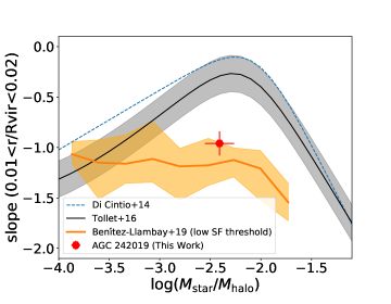
Figure 15: Implications of AGC 242019 for the stellar feedback model. Three lines represent different models about the dark-matter central density slope as a function of the $M_{\rm star}/M_{\rm halo}$ ratio. The red diamond symbol represents AGC 242019 in this study.

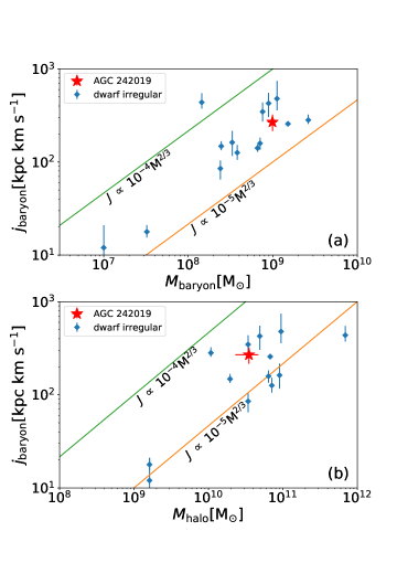
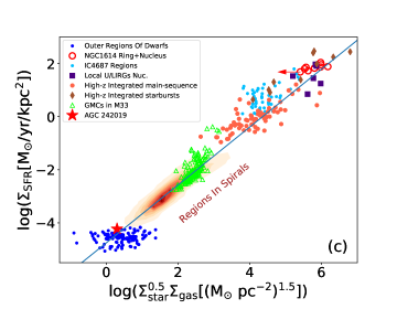
Figure 16: The implication of AGC 242019 for the UDG formation. a, The specific angular momentum of the baryons as a function of the baryonic mass, where red star symbol is AGC 242019 as compared to dwarf irregulars (Butler et al., 2017). b, the same as a, but versus the halo mass. c, The location of AGC 242019 in the extended Schmidt law (Shi et al., 2018).

5.2 Implications for the role of feedback on producing cored dark matter halo

It is found that the effect of baryonic feedback on the density profile of dark matter depends on the stellar-to-halo mass ratio ($M_{*}/M_{\rm halo}$) (e.g. Di Cintio et al., 2014; Tollet et al., 2016), as shown in Figure 15. In the low $M_{*}/M_{\rm halo}$ regime ($<$ 0.01%), the feedback is not strong enough to expel baryons and no dark-matter core forms. In the high $M_{*}/M_{\rm halo}$ regime ($>$ 3%), the significant contribution to the potential from baryonic matter cancels out the feedback effect and even produces a cuspier profile. In between, the stellar feedback can efficiently alter the density profile and a flattest density profile forms around $M_{*}/M_{\rm halo}$=0.6%. The above result is independent of model parameters such as star formation threshold, initial mass function, supernovae energy etc. However, AGC 242019 has a stellar mass of (1.37$\pm$0.05)$\times$10⁸ M_⊙  and a halo mass of (3.5$\pm$1.2)$\times$10¹⁰ M_⊙ , leading to $M_{*}/M_{\rm halo}$ of (0.39$\pm$0.13)% , which is close to the ratio where a flattest slope should form in simulations. AGC 242019 is thus inconsistent with the above $M_{*}/M_{\rm halo}$ dependence of the inner dark-matter profile.

Some other studies emphasize the importance of star formation threshold on the effect of the stellar feedback (e.g. Governato et al., 2010; Benítez-Llambay et al., 2019). If the threshold for gas to form stars is high, a large amount of gas can accumulate in the center of a halo and dominate the potential before star formation takes place. The subsequent feedback-driven massive outflows or repeated multiple outflows alter the orbits of dark matter to produce a dark-matter core. On the other hand, for low star formation threshold, gas is expelled by feedback before it contributes significantly to the potential. A dark-matter cuspy profile thus preserves. This scenario at least partly explains the formation of dark-matter cores in some simulations (Di Cintio et al., 2014; Fitts et al., 2017; Macciò et al., 2017) while not in others (Bose et al., 2019). The simulation by Benítez-Llambay et al. (2019) predicts an intact cuspy dark-matter density profile independent of the $M_{*}/M_{\rm halo}$ if star formation threshold is low. As shown in Figure 15, AGC 242019 is consistent with their prediction. As a UDG, AGC 242019 does have a low gas and stellar mass surface density with ongoing star formation as revealed by the GALEX far-UV image. This indicates that on sub-kpc scales star formation in AGC 242019 can proceed at a very low gas mass surface density that is on the order of 1 M_⊙/pc² or 0.4$\times$(100pc/$h$) cm^-3, where $h$ is the scale height of the gas disk. However, its star formation efficiency (SFR/gas=0.03 Gyr^-1) is much lower than that in spiral galaxies ($\sim$0.3 Gyr^-1) (Leroy et al., 2008; Shi et al., 2011), inconsistent with that adopted in the simulations. Therefore, low star formation threshold should not be simply the physical cause for a cuspy profile in AGC 242019.

Besides the star formation threshold, the duration of star formation may be also important as recognized in some simulations (Read et al., 2016a). As long as star formation proceeds long enough, e.g., $\sim$10 Gyr for a halo mass of 10⁹ M_⊙ and a longer timescale for a larger halo, a halo core always form. AGC 242019 has a halo mass of (3.5$\pm$1.2)$\times$10¹⁰ M_⊙ , and its low concentration implies late formation time (see next section), two of which may explain its cuspy profile given the above scenario.

5.3 Implications for formation of UDGs

UDGs are low-stellar-mass dwarfs but with sizes typical of spiral galaxies (Abraham & van Dokkum, 2014; Leisman et al., 2017). They were found in all environments including galaxy clusters, galaxy groups and field. Many mechanisms have been proposed to understand their origin: they may be normal dwarf galaxies but experience star-formation feedback that re-distributes gas and stars to larger radii (Governato et al., 2010; Di Cintio et al., 2014; Jiang et al., 2019); they may live in a high-spin dark matter halo with extended gas distributions and low efficiencies in converting gas into stars (Amorisco & Loeb, 2016); some environmental effects such as ram-pressure stripping or tidal puffing may be also important in formation of UDGs (Yozin & Bekki, 2015; Jiang et al., 2019).

The dark matter halo of AGC 242019 has a mass of (3.5$\pm$1.2)$\times$10¹⁰ M_⊙ , which is typical of a halo hosting a dwarf. This suggests that AGC 242019 is not a failed massive galaxy, unlike other UDGs found in clusters (van Dokkum et al., 2016; Beasley et al., 2016). Although UDGs may have diverse origins, our measurements are more reliable. In studies of van Dokkum et al. (2016) and Beasley et al. (2016), the halo mass was inferred from 1-2 velocity data-points by assuming a halo shape especially the concentration.

The cuspy halo of AGC 242019 also suggests that the feedback has not been strong over its history to expel a large amount of baryonic matter to large distances. Otherwise, a cored halo should have already formed like in other dwarf galaxies as suggested by feedback models (Navarro et al., 1996; Governato et al., 2010). AGC 242019 thus has experienced weak feedback over its history. This seems to be consistent with the deviation of UDGs from the Tully-Fisher relationship: gas and stars are not expelled out of the disk so that a UDG contain more baryons at a given maximum circular velocity that roughly represents the halo mass (Mancera Piña et al., 2020). AGC 242019 has a maximum circular velocity of 47 km s^-1  and a baryonic mass of (9.88$\pm$0.36)$\times$10⁸ M_⊙ , placing it slightly above the Tully-Fisher relationship too. With the accurate measurement of the halo mass, AGC 242019 is found to be off both the $M_{*}$ vs. $M_{\rm halo}$ and $M_{\rm baryon}$ vs. $M_{\rm halo}$ relationships (Santos-Santos et al., 2016). The low SFR of AGC 242019 also suggests weak ongoing stellar feedback as implied by the relationship between the SFR and the ionized gas velocity dispersion (e.g. Yu et al., 2019). Our regular velocity field with small non-circular motion as shown in § 4.2 is consistent with weak ongoing feedback too.

The halo of AGC 242019 has a small concentration of 2.0$\pm$0.36 , which is much smaller than the median concentration of 15 at the same halo mass in the local Universe as expected from simulations (Macciò et al., 2007). This difference is most likely because that AGC 242019 is an isolated halo that origins from a tiny initial density peak in the early time and collapses recently. It is found that the halo concentration decreases with later formation time (Zhao et al., 2003; Lu et al., 2006). A “young” halo thus suggests late formation of AGC 242019, which seems to be consistent with the findings of UDGs in cosmological simulations (Rong et al., 2017).

The specific angular momentum can be derived from the rotation curve combined with the stellar and gas mass profiles. The mass profiles were extended to 15 kpc following the same procedure that estimates the baryonic contribution to the rotation curve (see § 3.1.3 and § 3.1.4). The rotation curve is extended to 15 kpc too by combining the best-fitted NFW rotation curve plus the baryonic contribution. As shown in Figure 16 (a), it is found that AGC 242019 has an angular momentum that is consistent with dwarf irregular galaxies at the same baryonic mass (Butler et al., 2017). However, as discussed before, AGC 242019 has a higher baryon/halo mass ratio as compared to galaxies in general. We derived the halo masses of dwarf irregulars following Butler et al. (2017) and compared them with AGC 242019. As shown in Figure 16 (b), AGC 242019 still has a similar specific angular momentum at a given halo mass as compared to the average of dwarf irregulars. The result may be against the model that a UDG forms in a high-spin dark matter halo (Amorisco & Loeb, 2016).

As shown in § 5.2, AGC 242019 has a low star formation efficiency, consistent with the model of Amorisco & Loeb (2016). If placing it on the extended star formation law (Shi et al., 2011, 2018), we found that AGC 242019 follows the law as shown in Figure 16 (c). This suggests that its low star formation efficiency is regulated by its low stellar mass surface density.

In summary, AGC 242019 forms in a dwarf-size halo with late formation time. It has weak feedback, low star formation efficiency and a normal specific angular momentum of baryons at a given halo mass.

6 Conclusions

We have carried out the spatially-resolved mapping of gas dynamics toward a nearby UDG, AGC 242019. It is found that AGC 242019 has a cuspy dark matter halo at a high confidence, which demonstrates the validity of the cold dark matter paradigm on subgalactic scales. Our main conclusions are

(1) AGC 242019 has an overall regular velocity field. After subtracting the baryonic contribution, the rotation curve of dark matter is well fitted by the cuspy profile as described by the Navarro-Frenk-White (NFW) model, while the cored profiles including both the pseudo-isothermal and Burkert models are excluded. The result is robust against various systematic uncertainties.

(2) The central density slope of dark matter halo is found to be -(0.90$\pm$0.08)  at the innermost radius of 0.67 kpc.

(3) AGC 242019 poses challenges to alternatives of standard cold dark matter by constraining the particle mass of fuzzy dark matter to be $<$ 0.11$\times$10^-22 eV, or $>$ 3.3$\times$10^-22 eV , the cross section of self-interacting dark matter to be $<$ 1.63 cm²/g, and the particle mass of warm dark matter to be $>$ 0.23 keV, all of which are in tension with other constraints.

(4) AGC 242019 lies on the extrapolation of the radial acceleration relationship as defined by spirals and dwarf galaxies. However, the slope of the relationship defined by AGC 242019 is 0.15$\pm$0.11 , 3.2-$\sigma$ below the threshold (0.5) of the modified Newtonian dynamics.

(5) In the cold dark matter paradigm, the cuspy halo of AGC 242019 thus supports the feedback scenario that transforms cuspy halos to cored halos as frequently seen in other galaxies. However, the detailed physical process is unclear. The cuspy halo of AGC 242019 is inconsistent with the stellar-to-halo-mass-ratio dependent model, while consistent with the star-formation-threshold dependent model. But even for the later, the observed star formation efficiency (SFR/gas) is much lower than what is adopted in simulations. It may be consistent with the scenario that the duration of star formation is the key driver.

(6) As a UDG, AGC 242019 has a halo mass of (3.5$\pm$1.2)$\times$10¹⁰ M_⊙ , implying its formation in a dwarf-size halo. The cuspy halo further suggests weak feedback over the history. The small concentration of its halo is consistent with late formation time. Its specific angular momentum of baryons is consistent with the average of dwarf irregulars at a given halo/baryonic mass. Its star formation efficiency (SFR/gas) is low, probably due to the low stellar mass surface density.

Appendix A The full setup to run ^3DBarolo

In Table 6, the full list of the parameters to run ^3DBarolo is listed.

Table 6: The full parameter list for ^3DBarolo

Parameters	Values
Checking for bad channels in the cube……..[checkChannels]	false
Using Robust statistics?……………….[flagRobustStats]	true
Writing the mask to a fitsfile………………..[MAKEMASK]	false
Searching for sources in cube?………………….[SEARCH]	false
Smoothing the datacube?………………………..[SMOOTH]	false
Hanning smoothing the datacube?………………..[HANNING]	false
Writing a 3D model?……………………………[GALMOD]	false
Fitting a 3D model to the datacube?………………[3DFIT]	true
Number of radii…………………………….[NRADII]	7
Separation between radii (arcsec)…………….[RADSEP]	9
X center of the galaxy (pixel)…………………[XPOS]	415.19
Y center of the galaxy (pixel)…………………[YPOS]	405.49
Systemic velocity of the galaxy (km/s)………….[VSYS]	1840.46
Initial global rotation velocity (km/s)…………[VROT]	30
Initial global radial velocity (km/s)…………..[VRAD]	-1
Initial global velocity dispersion (km/s)………[VDISP]	5
Initial global inclination (degrees)…………….[INC]	69.90
Initial global position angle (degrees)…………..[PA]	2.0025
Scale height of the disk (arcsec)………………..[Z0]	0.7
Global column density of gas (atoms/cm2)………..[DENS]	-1
Parameters to be minimized…………………….[FREE]	VROT,VDISP,PA,INC
Type of mask…………………………………[MASK]	SEARCH
Side of the galaxy to be used………………….[SIDE]	B
Type of normalization…………………………[NORM]	LOCAL
Layer type along z direction………………….[LTYPE]	gaussian
Residuals to minimize………………………..[FTYPE]	chi-squared
Weighting function…………………………..[WFUNC]	uniform
Weight for blank pixels…………………….[BWEIGHT]	1
Minimization tolerance…………………………[TOL]	0.001
What side of the galaxy to be used……………..[SIDE]	B
Two stages minimization?…………………..[TWOSTAGE]	true
Degree of polynomial fitting angles?…………[POLYN]	bezier
Estimating errors?………………………[FLAGERRORS]	true
Redshift of the galaxy?……………………[REDSHIFT]	0
Computing asymmetric drift correction?………..[ADRIFT]	true
Overlaying mask to output plots?……………[PLOTMASK]	false
RMS noise to add to the model………………[NOISERMS]	false
Using cumulative rings during the fit?…….[CUMULATIVE]	false
Full parameter space for a pair of parameters…..[SPACEPAR]	false
Generating a 3D datacube with a wind model?……..[GALWIND]	false
Fitting velocity field with a ring model?…………[2DFIT]	false
Deriving radial intensity profile?……………..[ELLPROF]	false

Appendix B Different runs of ^3DBarolo

In Figure 17, we compared the derived rotation velocities (before the pressure support correction) and velocity dispersions by running ^3DBarolo with both sides of the gas disk, only the receding side and only the approaching side, respectively.

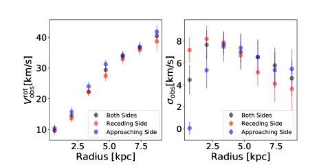
Figure 17: The comparison in the derived rotation velocities and velocity dispersions by using both sides, only the receding side and only the approaching side of HI data, respectively.

References

- Abraham & van Dokkum (2014) Abraham, R. G., & van Dokkum, P. G. 2014, PASP, 126, 55, doi: 10.1086/674875
- Adams et al. (2014) Adams, J. J., Simon, J. D., Fabricius, M. H., et al. 2014, ApJ, 789, 63, doi: 10.1088/0004-637X/789/1/63
- Amorisco & Loeb (2016) Amorisco, N. C., & Loeb, A. 2016, MNRAS, 459, L51, doi: 10.1093/mnrasl/slw055
- Avila-Reese et al. (2001) Avila-Reese, V., Colín, P., Valenzuela, O., D’Onghia, E., & Firmani, C. 2001, ApJ, 559, 516, doi: 10.1086/322411
- Bailin & Steinmetz (2005) Bailin, J., & Steinmetz, M. 2005, ApJ, 627, 647, doi: 10.1086/430397
- Beasley et al. (2016) Beasley, M. A., Romanowsky, A. J., Pota, V., et al. 2016, ApJ, 819, L20, doi: 10.3847/2041-8205/819/2/L20
- Begeman (1989) Begeman, K. G. 1989, A&A, 223, 47
- Begeman et al. (1991) Begeman, K. G., Broeils, A. H., & Sanders, R. H. 1991, MNRAS, 249, 523, doi: 10.1093/mnras/249.3.523
- Bell et al. (2003) Bell, E. F., McIntosh, D. H., Katz, N., & Weinberg, M. D. 2003, ApJS, 149, 289, doi: 10.1086/378847
- Benítez-Llambay et al. (2019) Benítez-Llambay, A., Frenk, C. S., Ludlow, A. D., & Navarro, J. F. 2019, MNRAS, 488, 2387, doi: 10.1093/mnras/stz1890
- Blitz & Rosolowsky (2006) Blitz, L., & Rosolowsky, E. 2006, ApJ, 650, 933, doi: 10.1086/505417
- Bose et al. (2019) Bose, S., Frenk, C. S., Jenkins, A., et al. 2019, MNRAS, 486, 4790, doi: 10.1093/mnras/stz1168
- Bureau & Carignan (2002) Bureau, M., & Carignan, C. 2002, AJ, 123, 1316, doi: 10.1086/338899
- Burkert (1995) Burkert, A. 1995, ApJ, 447, L25, doi: 10.1086/309560
- Butler et al. (2017) Butler, K. M., Obreschkow, D., & Oh, S.-H. 2017, ApJ, 834, L4, doi: 10.3847/2041-8213/834/1/L4
- Carignan & Beaulieu (1989) Carignan, C., & Beaulieu, S. 1989, ApJ, 347, 760, doi: 10.1086/168167
- Chang & Necib (2020) Chang, L. J., & Necib, L. 2020, arXiv e-prints, arXiv:2009.00613. https://arxiv.org/abs/2009.00613
- Childress et al. (2014) Childress, M., Vogt, F., Nielsen, J., & Sharp, R. 2014, PyWiFeS: Wide Field Spectrograph data reduction pipeline. http://ascl.net/1402.034
- de Blok et al. (2001) de Blok, W. J. G., McGaugh, S. S., Bosma, A., & Rubin, V. C. 2001, ApJ, 552, L23, doi: 10.1086/320262
- Dey et al. (2019) Dey, A., Schlegel, D. J., Lang, D., et al. 2019, AJ, 157, 168, doi: 10.3847/1538-3881/ab089d
- Di Cintio et al. (2014) Di Cintio, A., Brook, C. B., Macciò, A. V., et al. 2014, MNRAS, 437, 415, doi: 10.1093/mnras/stt1891
- Di Teodoro & Fraternali (2015) Di Teodoro, E. M., & Fraternali, F. 2015, MNRAS, 451, 3021, doi: 10.1093/mnras/stv1213
- Einasto (1965) Einasto, J. 1965, Trudy Astrofizicheskogo Instituta Alma-Ata, 5, 87
- Elbert et al. (2015) Elbert, O. D., Bullock, J. S., Garrison-Kimmel, S., et al. 2015, MNRAS, 453, 29, doi: 10.1093/mnras/stv1470
- Evans et al. (2009) Evans, N. W., An, J., & Walker, M. G. 2009, MNRAS, 393, L50, doi: 10.1111/j.1745-3933.2008.00596.x
- Fitts et al. (2017) Fitts, A., Boylan-Kolchin, M., Elbert, O. D., et al. 2017, MNRAS, 471, 3547, doi: 10.1093/mnras/stx1757
- Ghigna et al. (2000) Ghigna, S., Moore, B., Governato, F., et al. 2000, ApJ, 544, 616, doi: 10.1086/317221
- Governato et al. (2010) Governato, F., Brook, C., Mayer, L., et al. 2010, Nature, 463, 203, doi: 10.1038/nature08640
- Harvey et al. (2015) Harvey, D., Massey, R., Kitching, T., Taylor, A., & Tittley, E. 2015, Science, 347, 1462, doi: 10.1126/science.1261381
- Hayashi et al. (2020) Hayashi, K., Chiba, M., & Ishiyama, T. 2020, arXiv e-prints, arXiv:2007.13780. https://arxiv.org/abs/2007.13780
- Haynes et al. (2018) Haynes, M. P., Giovanelli, R., Kent, B. R., et al. 2018, ApJ, 861, 49, doi: 10.3847/1538-4357/aac956
- Hogan & Dalcanton (2000) Hogan, C. J., & Dalcanton, J. J. 2000, Phys. Rev. D, 62, 063511, doi: 10.1103/PhysRevD.62.063511
- Hu et al. (2000) Hu, W., Barkana, R., & Gruzinov, A. 2000, Phys. Rev. Lett., 85, 1158, doi: 10.1103/PhysRevLett.85.1158
- Iorio et al. (2017) Iorio, G., Fraternali, F., Nipoti, C., et al. 2017, MNRAS, 466, 4159, doi: 10.1093/mnras/stw3285
- Jardel et al. (2013) Jardel, J. R., Gebhardt, K., Fabricius, M. H., Drory, N., & Williams, M. J. 2013, ApJ, 763, 91, doi: 10.1088/0004-637X/763/2/91
- Jarrett et al. (2013) Jarrett, T. H., Masci, F., Tsai, C. W., et al. 2013, AJ, 145, 6, doi: 10.1088/0004-6256/145/1/6
- Jester et al. (2005) Jester, S., Schneider, D. P., Richards, G. T., et al. 2005, AJ, 130, 873, doi: 10.1086/432466
- Jiang et al. (2019) Jiang, F., Dekel, A., Freundlich, J., et al. 2019, MNRAS, 487, 5272, doi: 10.1093/mnras/stz1499
- Jing & Suto (2002) Jing, Y. P., & Suto, Y. 2002, ApJ, 574, 538, doi: 10.1086/341065
- Jobin & Carignan (1990) Jobin, M., & Carignan, C. 1990, AJ, 100, 648, doi: 10.1086/115548
- Kahlhoefer et al. (2015) Kahlhoefer, F., Schmidt-Hoberg, K., Kummer, J., & Sarkar, S. 2015, MNRAS, 452, L54, doi: 10.1093/mnrasl/slv088
- Kaplinghat et al. (2016) Kaplinghat, M., Tulin, S., & Yu, H.-B. 2016, Phys. Rev. Lett., 116, 041302, doi: 10.1103/PhysRevLett.116.041302
- Kelly (2007) Kelly, B. C. 2007, ApJ, 665, 1489, doi: 10.1086/519947
- Knebe & Wießner (2006) Knebe, A., & Wießner, V. 2006, PASA, 23, 125, doi: 10.1071/AS06013
- Kuzio de Naray & Kaufmann (2011) Kuzio de Naray, R., & Kaufmann, T. 2011, MNRAS, 414, 3617, doi: 10.1111/j.1365-2966.2011.18656.x
- Kuzio de Naray et al. (2008) Kuzio de Naray, R., McGaugh, S. S., & de Blok, W. J. G. 2008, ApJ, 676, 920, doi: 10.1086/527543
- Kuzio de Naray et al. (2009) Kuzio de Naray, R., McGaugh, S. S., & Mihos, J. C. 2009, ApJ, 692, 1321, doi: 10.1088/0004-637X/692/2/1321
- Lake et al. (1990) Lake, G., Schommer, R. A., & van Gorkom, J. H. 1990, AJ, 99, 547, doi: 10.1086/115349
- Leisman et al. (2017) Leisman, L., Haynes, M. P., Janowiecki, S., et al. 2017, ApJ, 842, 133, doi: 10.3847/1538-4357/aa7575
- Lelli et al. (2017) Lelli, F., McGaugh, S. S., Schombert, J. M., & Pawlowski, M. S. 2017, ApJ, 836, 152, doi: 10.3847/1538-4357/836/2/152
- Leroy et al. (2008) Leroy, A. K., Walter, F., Brinks, E., et al. 2008, AJ, 136, 2782, doi: 10.1088/0004-6256/136/6/2782
- Lovell et al. (2014) Lovell, M. R., Frenk, C. S., Eke, V. R., et al. 2014, MNRAS, 439, 300, doi: 10.1093/mnras/stt2431
- Lu et al. (2006) Lu, Y., Mo, H. J., Katz, N., & Weinberg, M. D. 2006, MNRAS, 368, 1931, doi: 10.1111/j.1365-2966.2006.10270.x
- Macciò et al. (2007) Macciò, A. V., Dutton, A. A., van den Bosch, F. C., et al. 2007, MNRAS, 378, 55, doi: 10.1111/j.1365-2966.2007.11720.x
- Macciò et al. (2017) Macciò, A. V., Frings, J., Buck, T., et al. 2017, MNRAS, 472, 2356, doi: 10.1093/mnras/stx2048
- Macciò et al. (2012) Macciò, A. V., Paduroiu, S., Anderhalden, D., Schneider, A., & Moore, B. 2012, MNRAS, 424, 1105, doi: 10.1111/j.1365-2966.2012.21284.x
- Mancera Piña et al. (2020) Mancera Piña, P. E., Fraternali, F., Oman, K. A., et al. 2020, MNRAS, 495, 3636, doi: 10.1093/mnras/staa1256
- McMullin et al. (2007) McMullin, J. P., Waters, B., Schiebel, D., Young, W., & Golap, K. 2007, in Astronomical Society of the Pacific Conference Series, Vol. 376, Astronomical Data Analysis Software and Systems XVI, ed. R. A. Shaw, F. Hill, & D. J. Bell, 127
- Meidt et al. (2014) Meidt, S. E., Schinnerer, E., van de Ven, G., et al. 2014, ApJ, 788, 144, doi: 10.1088/0004-637X/788/2/144
- Milgrom (1983) Milgrom, M. 1983, ApJ, 270, 365, doi: 10.1086/161130
- Moore (1994) Moore, B. 1994, Nature, 370, 629, doi: 10.1038/370629a0
- Moore et al. (1998) Moore, B., Governato, F., Quinn, T., Stadel, J., & Lake, G. 1998, ApJ, 499, L5, doi: 10.1086/311333
- Mould et al. (2000) Mould, J. R., Huchra, J. P., Freedman, W. L., et al. 2000, ApJ, 529, 786, doi: 10.1086/308304
- Navarro et al. (1996) Navarro, J. F., Eke, V. R., & Frenk, C. S. 1996, MNRAS, 283, L72, doi: 10.1093/mnras/283.3.L72
- Navarro et al. (1997) Navarro, J. F., Frenk, C. S., & White, S. D. M. 1997, ApJ, 490, 493, doi: 10.1086/304888
- Nipoti & Binney (2015) Nipoti, C., & Binney, J. 2015, MNRAS, 446, 1820, doi: 10.1093/mnras/stu2217
- Oh et al. (2011) Oh, S.-H., de Blok, W. J. G., Brinks, E., Walter, F., & Kennicutt, Robert C., J. 2011, AJ, 141, 193, doi: 10.1088/0004-6256/141/6/193
- Oh et al. (2015) Oh, S.-H., Hunter, D. A., Brinks, E., et al. 2015, AJ, 149, 180, doi: 10.1088/0004-6256/149/6/180
- Oman et al. (2019) Oman, K. A., Marasco, A., Navarro, J. F., et al. 2019, MNRAS, 482, 821, doi: 10.1093/mnras/sty2687
- Osterbrock & Ferland (2006) Osterbrock, D. E., & Ferland, G. J. 2006, Astrophysics of gaseous nebulae and active galactic nuclei
- Pineda et al. (2017) Pineda, J. C. B., Hayward, C. C., Springel, V., & Mendes de Oliveira, C. 2017, MNRAS, 466, 63, doi: 10.1093/mnras/stw3004
- Randall et al. (2008) Randall, S. W., Markevitch, M., Clowe, D., Gonzalez, A. H., & Bradač, M. 2008, ApJ, 679, 1173, doi: 10.1086/587859
- Read et al. (2016a) Read, J. I., Agertz, O., & Collins, M. L. M. 2016a, MNRAS, 459, 2573, doi: 10.1093/mnras/stw713
- Read et al. (2016b) Read, J. I., Iorio, G., Agertz, O., & Fraternali, F. 2016b, MNRAS, 462, 3628, doi: 10.1093/mnras/stw1876
- Read et al. (2019) Read, J. I., Walker, M. G., & Steger, P. 2019, MNRAS, 484, 1401, doi: 10.1093/mnras/sty3404
- Riess et al. (2016) Riess, A. G., Macri, L. M., Hoffmann, S. L., et al. 2016, ApJ, 826, 56, doi: 10.3847/0004-637X/826/1/56
- Rocha et al. (2013) Rocha, M., Peter, A. H. G., Bullock, J. S., et al. 2013, MNRAS, 430, 81, doi: 10.1093/mnras/sts514
- Rong et al. (2017) Rong, Y., Guo, Q., Gao, L., et al. 2017, MNRAS, 470, 4231, doi: 10.1093/mnras/stx1440
- Salvatier et al. (2016) Salvatier, J., Wieckiâ, T. V., & Fonnesbeck, C. 2016, PyMC3: Python probabilistic programming framework. http://ascl.net/1610.016
- Santos-Santos et al. (2016) Santos-Santos, I. M., Brook, C. B., Stinson, G., et al. 2016, MNRAS, 455, 476, doi: 10.1093/mnras/stv2335
- Schive et al. (2014) Schive, H.-Y., Chiueh, T., & Broadhurst, T. 2014, Nature Physics, 10, 496, doi: 10.1038/nphys2996
- Schoenmakers et al. (1997) Schoenmakers, R. H. M., Franx, M., & de Zeeuw, P. T. 1997, MNRAS, 292, 349, doi: 10.1093/mnras/292.2.349
- Schombert et al. (2019) Schombert, J., McGaugh, S., & Lelli, F. 2019, MNRAS, 483, 1496, doi: 10.1093/mnras/sty3223
- Shi et al. (2011) Shi, Y., Helou, G., Yan, L., et al. 2011, ApJ, 733, 87, doi: 10.1088/0004-637X/733/2/87
- Shi et al. (2018) Shi, Y., Yan, L., Armus, L., et al. 2018, ApJ, 853, 149, doi: 10.3847/1538-4357/aaa3e6
- Spekkens et al. (2005) Spekkens, K., Giovanelli, R., & Haynes, M. P. 2005, AJ, 129, 2119, doi: 10.1086/429592
- Spergel & Steinhardt (2000) Spergel, D. N., & Steinhardt, P. J. 2000, Phys. Rev. Lett., 84, 3760, doi: 10.1103/PhysRevLett.84.3760
- Telford et al. (2020) Telford, O. G., Dalcanton, J. J., Williams, B. F., et al. 2020, ApJ, 891, 32, doi: 10.3847/1538-4357/ab701c
- Tollet et al. (2016) Tollet, E., Macciò, A. V., Dutton, A. A., et al. 2016, MNRAS, 456, 3542, doi: 10.1093/mnras/stv2856
- Trachternach et al. (2008) Trachternach, C., de Blok, W. J. G., Walter, F., Brinks, E., & Kennicutt, R. C., J. 2008, AJ, 136, 2720, doi: 10.1088/0004-6256/136/6/2720
- Tulin & Yu (2018) Tulin, S., & Yu, H.-B. 2018, Phys. Rep., 730, 1, doi: 10.1016/j.physrep.2017.11.004
- van Dokkum et al. (2016) van Dokkum, P., Abraham, R., Brodie, J., et al. 2016, ApJ, 828, L6, doi: 10.3847/2041-8205/828/1/L6
- Vehtari et al. (2015) Vehtari, A., Gelman, A., & Gabry, J. 2015, arXiv e-prints, arXiv:1507.04544. https://arxiv.org/abs/1507.04544
- Walker et al. (2015) Walker, M. G., Olszewski, E. W., & Mateo, M. 2015, MNRAS, 448, 2717, doi: 10.1093/mnras/stv099
- Wang et al. (2020) Wang, J., Bose, S., Frenk, C. S., et al. 2020, Nature, 585, 39, doi: 10.1038/s41586-020-2642-9
- Weinberg et al. (2015) Weinberg, D. H., Bullock, J. S., Governato, F., Kuzio de Naray, R., & Peter, A. H. G. 2015, Proceedings of the National Academy of Science, 112, 12249, doi: 10.1073/pnas.1308716112
- Wright et al. (2010) Wright, E. L., Eisenhardt, P. R. M., Mainzer, A. K., et al. 2010, AJ, 140, 1868, doi: 10.1088/0004-6256/140/6/1868
- Yozin & Bekki (2015) Yozin, C., & Bekki, K. 2015, MNRAS, 452, 937, doi: 10.1093/mnras/stv1073
- Yu et al. (2019) Yu, X., Shi, Y., Chen, Y., et al. 2019, MNRAS, 486, 4463, doi: 10.1093/mnras/stz1146
- Zavala et al. (2013) Zavala, J., Vogelsberger, M., & Walker, M. G. 2013, MNRAS, 431, L20, doi: 10.1093/mnrasl/sls053
- Zhao et al. (2003) Zhao, D. H., Mo, H. J., Jing, Y. P., & Börner, G. 2003, MNRAS, 339, 12, doi: 10.1046/j.1365-8711.2003.06135.x
- Zibetti et al. (2009) Zibetti, S., Charlot, S., & Rix, H.-W. 2009, MNRAS, 400, 1181, doi: 10.1111/j.1365-2966.2009.15528.x