Regression Discontinuity Design with Many Thresholds

Abstract

Numerous empirical studies employ regression discontinuity designs with multiple cutoffs and heterogeneous treatments. A common practice is to normalize all the cutoffs to zero and estimate one effect. This procedure identifies the average treatment effect (ATE) on the observed distribution of individuals local to existing cutoffs. However, researchers often want to make inferences on more meaningful ATEs, computed over general counterfactual distributions of individuals, rather than simply the observed distribution of individuals local to existing cutoffs. This paper proposes a consistent and asymptotically normal estimator for such ATEs when heterogeneity follows a non-parametric function of cutoff characteristics in the sharp case. The proposed estimator converges at the minimax optimal rate of root-$n$ for a specific choice of tuning parameters. Identification in the fuzzy case, with multiple cutoffs, is impossible unless heterogeneity follows a finite-dimensional function of cutoff characteristics. Under parametric heterogeneity, this paper proposes an ATE estimator for the fuzzy case that optimally combines observations to maximize its precision.

Keywords: Regression Discontinuity, Multiple Cutoffs, Average Treatment Effect, Peer-effects

JEL Classification: C14, C21, C52, I21.

1 Introduction

Applications of regression discontinuity design (RDD) have become increasingly popular in economics since the late 1990s (Black (1999), Angrist and Lavy (1999), and Van der Klaauw (2002)). One of RDD’s main advantages is identification of a local causal effect under minimal functional form assumptions. More recently, with increasing availability of richer data sets, there have been many applications with multiple cutoffs and treatments (for example, Black et al. (2007), Egger and Koethenbuerger (2010), De La Mata (2012), Pop-Eleches and Urquiola (2013)). Existing one-cutoff RDD methods applied to each individual cutoff produce many local effects that are estimated using only a few observations near each cutoff. Researchers often prefer one takeaway summary effect that is more precisely estimated by pooling all the data. The meaning of a summary effect crucially depends on heterogeneity assumptions and weights imposed on the different local effects.

Applied studies with multiple cutoffs often normalize all cutoffs to zero and use the one-cutoff estimator. This normalization procedure estimates an average of local treatment effects weighted by the relative density of individuals near each of the cutoffs (Cattaneo et al. (2016), Proposition 3). Such an average effect would be a meaningful summary measure only in two cases: (i) local treatment effects are all identical and the weighting scheme does not matter; or (ii) local treatment effects are heterogeneous but the researcher is only interested in the average effect on the individuals near the existing cutoffs. However, researchers are often interested in combining observed data with assumptions weaker than (i) to make inferences on counterfactual scenarios more general than (ii).

This paper proposes a novel estimation procedure for average treatment effects (ATE). These ATEs are more valuable summary measures than the average effect estimated by the normalization procedure described above for two reasons. First, the researcher explicitly chooses the counterfactual distribution of the ATE, and this distribution may include individuals at or between existing cutoffs. Second, the researcher does not need to assume any specific functional form for the heterogeneity of treatment effects across different cutoffs. As an example of an application, suppose we are interested in estimating the effect of Medicaid benefits on health care utilization. Medicaid eligibility is triggered by income cutoffs that vary across states. Existing one-cutoff RDD methods identify the average effect on individuals with income equal to the income cutoffs. However, most interesting policy questions require the average effect over the entire range of income values in the data.

The framework for RDD with many thresholds is introduced here using a simple example based on the work of Pop-Eleches and Urquiola (2013), PU from now on. Using a wealth of variation of cutoffs from high school assignments in Romania, PU provide rigorous evidence of the impacts of attending a better school on students’ academic performance. The economic logic of this application is briefly summarized as follows. A central planner assigns students to high schools based on their scores from a placement test. High schools have limited capacities and are ranked by their qualities. The central planner ranks students by their scores and assigns each of them to the best school available. Each student $i$ submits her score $X_{i}$ (forcing variable) to the central planner who, based on the entire distribution of scores, determines a minimum test score $c_{j}$ (cutoff) for admission to each high school $j$. The quality of high school $j$ is denoted $d_{j}$ (treatment dose).

The RDD assignment is assumed sharp for now. That is, students attend the best high school available to them based on their score and the cutoffs that apply to them. As the test score crosses an admission threshold $c_{j}$, the quality of the school the student attends changes from $d_{j-1}$ to $d_{j}$. Local average effects are denoted by $\mathbb{E}[Y_{i}(d_{j})-Y_{i}(d_{j-1})|X_{i}=c_{j}]=\beta(c_{j},d_{j-1},d_{j})$, where $Y_{i}(d)$ is the potential academic achievement student $i$ has if attending a high school of quality $d$, and $\beta(c,d,d^{\prime})$ is the treatment effect function. Heterogeneity of local effects comes from values of cutoffs and treatment doses that change across the different cutoffs. PU give a particularly illustrative application, because it exhibits sufficient variation in cutoff and treatment doses to generate ATEs with substantially greater economic relevance than the typical average based on normalizing all of the cutoffs to zero.

Numerous other examples of RDD with multiple cutoffs and treatments exist in different fields of economics. For instance, Egger and Koethenbuerger (2010) study the effect of the size of city government councils on municipal expenditures, where council size is determined by population cutoffs. De La Mata (2012) estimates the effects of Medicaid benefits on health care utilization, where Medicaid eligibility is triggered by income cutoffs that vary across states. Agarwal et al. (2017) and De Giorgi et al. (2017) look at multiple cutoffs on credit scores, used by banks to make credit decisions. Education economics also provides a variety of applications. Angrist and Lavy (1999) and Hoxby (2000) use class size rules to estimate the impact of class size on student achievement. Hoxby (2000) utilizes variation in cutoff values from specific school district class size rules. Several researchers exploit different school starting dates to estimate the impact of educational attainment on various outcomes, for example, Dobkin and Ferreira (2010), and McCrary and Royer (2011). Duflo et al. (2011) analyze school cohorts that are split into low and high-achieving classes based on test scores, where each school has its own cutoff score. Garibaldi et al. (2012) look at different income cutoffs that determine tuition subsidies to study the impact of tuition payment on the probability of late graduation from university. In short, despite many applications with variation in cutoffs and treatment doses, a lack of theory on how to combine observations from all cutoffs impedes our ability to estimate economically-relevant average effects.

Whether local effects can be combined into an average effect depends on how comparable the researcher believes these effects are. The comparability of local treatment effects essentially depends on the heterogeneity of treatment doses and on the heterogeneity of the treatment effect function $\beta(c,d,d^{\prime})$. This paper considers two types of assumptions regarding these two aspects of heterogeneity. The first heterogeneity assumption says that treatment doses are credibly quantifiable by some variable $d$. For example, PU find behavioral evidence that average student performance at each school is a good summary measure for school quality. Another example is the case of a single treatment being triggered by varying cutoffs, as when each state has its own income threshold for Medicaid coverage. The second heterogeneity assumption specifies a parametric functional form for $\beta(c,d,d^{\prime})$ guided by economic theory or a priori knowledge of the researcher. For example, in a class size application like Hoxby’s (2000), a functional form based on Lazear’s (2001) model of achievement can be derived as a function of class size. Another example is given by Bajari et al. (2017) who present a principal-agent model to study how insurers reimburse hospitals. The marginal reimbursement rate is discontinuous on health expenditures.

This paper proposes a consistent and asymptotically normal estimator for the ATE of a counterfactual distribution of treatment assignments specified by the researcher. A counterfactual policy scenario specifies the distribution of $(c,d,d^{\prime})$, and the ATE is the integral of $\beta(c,d,d^{\prime})$ weighted by such a distribution. The ability to predict effects of counterfactual policies depends crucially on assuming that the distribution of potential outcomes $Y_{i}(d)$ does not depend on the initial schedule of cutoff-dose values. This policy invariance assumption, along with the first heterogeneity assumption, allows the researcher to choose counterfactual distributions with support more general than the discrete set of cutoff-dose values observed in the data.

The estimator proposed in this paper approximates the ATE integral by averaging estimates of $\beta(c,d,d^{\prime})$ at existing cutoffs using a proper weighting scheme. Under the first heterogeneity assumption with $\beta(c,d,d^{\prime})$ non-parametric, the proposed ATE estimator is shown to be consistent and asymptotically normal. This result is novel, because estimation of the non-parametric function $\beta(c,d,d^{\prime})$ is only possible at deterministic points of the domain, and that creates an additional source of bias. Asymptotic normality requires both the number of observations and cutoffs to grow to infinity, and I provide sufficient conditions on their rate of growth. I demonstrate that the minimax rate of ATE estimation in this setting is root-$n$, and that the proposed estimator attains the minimax optimal rate for a specific choice of tuning parameters. This extends the previous literature on minimax optimality of non-parametric estimation of regression functions at a boundary point to estimation of averages of these regression functions.

Many applications of RDD with multiple cutoffs are, in fact, fuzzy rather than sharp. In the high school assignment example, a student may choose to attend a high school other than the school she is originally eligible to attend. Multiple treatments result in multiple compliance behaviors, and one-cutoff identification results do not apply. Building on classic definitions of compliance behaviors (Imbens and Rubin (1997)), I define compliance groups in terms of changes in treatment eligibility and receipt. “Ever-compliers” are those whose treatment received changes if and only if it changes to the treatment dose for which they become eligible for. I assume that individuals never change into a treatment dose different from the dose of eligibility, a “no-defiance” condition. In the high school example, if the test score of a student currently in school B increases so as to grant her access to school A, no-defiance implies she either chooses to attend school A or stay at school B, and that she is not triggered to attend some other school C.

This paper shows that even local identification in fuzzy RDD with finite multiple treatments is impossible unless the class of treatment effect functions of ever-compliers is restricted to a finite-dimensional class. Important empirical analyses of fuzzy RDD with multiple treatments include those of Angrist and Lavy (1999), Chen and Van der Klaauw (2008), and Hoekstra (2009); nevertheless, this is the first paper to define compliance and study causal identification in a general framework for multi-cutoff fuzzy RDD. This framework lays out conditions for the interpretation of two-stage least squares (2SLS) estimates in applications of multi-cutoff fuzzy RDD, a common practice in applied work. The second heterogeneity assumption states that the treatment effect function is of a parametric class. This assumption allows for consistent and asymptotically normal estimation of ATEs on ever-compliers. It also results in efficiency gains, because observations are optimally combined across cutoffs to minimize the mean squared error (MSE) of the ATE estimator.

The rapid growth in the number of applications of RDD in economics in the late 1990s was accompanied by substantial theoretical contributions for inference in the one-cutoff case. Identification and estimation in the sharp and fuzzy cases were formalized by Hahn et al. (2001). Fan and Gijbels (1996) and Porter (2003) demonstrated low-order bias and rate optimality of the local polynomial estimator. Recent theoretical contributions have addressed the optimal bandwidth choice (Imbens and Kalyanaraman (2012)), alternative asymptotic approximations with better finite sample properties (Calonico et al. (2014)), quantile treatment effects (Frandsen et al. (2012)), kink treatment effects (Dong (2018b)), and the difficulty of uniform inference (Bertanha and Moreira (2019)).

The contribution of this paper is more closely related to the study of treatment effect extrapolation of Angrist (2004), Bertanha and Imbens (2019), Dong and Lewbel (2015), Angrist and Rokkanen (2015), and Rokkanen (2015). These last two authors use observations on additional covariates. They restrict the relationship between the heterogeneity of treatment effects after conditioning on these covariates to obtain identification away from the cutoff. This paper differs from these other contributions, because the variation of multiple cutoffs and doses identify ATEs over distributions of individuals both between and at cutoffs, without additional covariates.

The remainder of this paper is organized as follows. Section 2 presents the notation and lays out basic assumptions. Section 3 describes the ATE estimator for the sharp case and proves asymptotic normality. It is divided into two sub-sections. Section 3.1 treats ATEs of discrete counterfactual distributions, which is a straightforward generalization of one-cutoff RDD. Section 3.2 is novel; it studies ATEs of continuous counterfactual distributions under the first heterogeneity assumption. Section 4 analyzes the fuzzy case. Appendix A contains all proofs. Supplemental Appendix B collects auxiliary results to the proofs in Appendix A.

2 Setup

This section sets up the framework for RDD with multiple cutoffs. There are $P$ sub-populations of individuals indexed by $p=1,\ldots,P$. An example of a sub-population may be a town-year in the high school application, or a state in the Medicaid example. Each individual $i$ in sub-population $p$ is fully characterized by a vector of random variables $(X_{i,p},U_{i,p})$ drawn iid across $i$ from each sub-population. The forcing variable $X_{i,p}$ is a scalar score that governs eligibility for treatment, and it lives in a compact interval $\mathcal{X}=[\underline{\mathcal{X}},\overline{\mathcal{X}}]$; $U_{i,p}$ is a vector of unobserved heterogeneity. Individual $(i,p)$ receives a treatment dose $D_{i,p}$ from a set of possible treatments $\mathcal{D}$. The outcome variable $Y_{i,p}$ is determined by a function $\mathbb{Y}$ of the individual characteristics and treatment,

$$Y_{i,p}=\mathbb{Y}(X_{i,p},D_{i,p},U_{i,p}).$$ (1)

I start with the simpler sharp RDD setting and defer the fuzzy RDD case to Section 4. In the sharp case, the treatment received by the individual is a deterministic function of the forcing variable. For an individual with forcing variable $X_{i,p}$ close to a cutoff $c$, the treatment dose is $d$ if $X_{i,p}<c$, or $d^{\prime}$ if $X_{i,p}\geq c$. Hahn et al. (2001) demonstrate that continuity of the conditional mean of outcomes is sufficient to identify average causal effects for individuals local to the cutoff $c$.

Lemma 1.

Assume that $\mathbb{E}[\mathbb{Y}(X_{i,p},d,U_{i,p})|X_{i,p}=x]$ is a continuous function of $x$ for the treatment doses $d$ and $d^{\prime}$ in the neighborhood of the cutoff $c$. Then, the average causal effect for individuals with $X_{i,p}=c$ is identified:

$$\mathbb{E}\left[\left.\mathbb{Y}(X_{i,p},d^{\prime},U_{i,p})-\mathbb{Y}(X_{i,p},d,U_{i,p})~{}\right|~{}X_{i,p}=c\right]$$

$$\hskip 56.9055pt=\lim_{e\downarrow 0}\Big{\{}~{}\mathbb{E}[Y_{i,p}~{}|~{}X_{i,p}=c+e]-\mathbb{E}[Y_{i,p}~{}|~{}X_{i,p}=c-e]~{}\Big{\}}.$$ (2)

Lemma 1 generalizes to the case of multiple cutoffs and treatments under the assumption of continuity of $\mathbb{E}[\mathbb{Y}(X_{i,p},d,U_{i,p})|X_{i,p}=x]$ as a function of $x$ for every $d\in\mathcal{D}$. Many cutoffs arise because data sets may have many sub-populations with few cutoffs (e.g. Medicaid benefit with one cutoff per state, many states); or few sub-populations with many cutoffs (e.g. Romanian high schools with one town and many schools). The ability to exploit variation in cutoff-dose values relies on the following pooling assumption. [assumptions.tex]assu00A

Assumption LABEL:assu_pool does not restrict average outcomes to be the same across different sub-populations. It is less restrictive than common specifications for pooling data in applied work, for example, time-trends and sub-population fixed effects. The pooling assumption says that individuals with the same forcing variable that undergo the same change in treatment have the same average response across different sub-populations. The rest of the paper builds on Assumption LABEL:assu_pool, and it becomes irrelevant to distinguish sub-populations. Thus, I drop the subscript $p$ and focus on the case of one population with multiple cutoffs.

The cutoffs are ordered such that $c_{1}<c_{2}<\ldots<c_{K}$. Sharp RDD means that an individual with forcing variable $X_{i}$ is deterministically assigned to a treatment dose $D_{i}=D(X_{i})$ according to the following rule:

$$D(x)=\left\{\begin{array}[]{cc}d_{0}&\text{ if }c_{0}\leq x<c_{1}\\ d_{1}&\text{ if }c_{1}\leq x<c_{2}\\ \vdots\\ d_{K}&\text{ if }c_{K}\leq x\leq c_{K+1}\end{array}\right.$$ (7)

where $c_{0}=\underline{\mathcal{X}}$, and $c_{K+1}=\overline{\mathcal{X}}$. Each cutoff is characterized by three variables: the scalar threshold $c_{j}$; the treatment dose $d_{j-1}$ the individual receives if $c_{j-1}\leq X_{i}<c_{j}$; and the treatment dose $d_{j}$ the individual receives if $c_{j}\leq X_{i}<c_{j+1}$. Let $\bm{\mathrm{c}}_{j}=(c_{j},d_{j-1},d_{j})$. The schedule of cutoffs and treatment doses is given by the non-random set $\mathcal{C}_{K}=\left\{\bm{\mathrm{c}}_{j}\right\}_{j=1}^{K}$. The richness of set $\mathcal{C}_{K}$ increases as the researcher collects more data.

The data generating process is summarized as follows. Values for the forcing variable $X_{i}$ and heterogeneity $U_{i}$ are drawn iid $i=1,...,n$ from a joint distribution. Given $D(x)$, these $n$ individuals are assigned to different treatment doses $D_{i}=D(X_{i})$. The observed outcome is determined by $Y_{i}=\mathbb{Y}(X_{i},D_{i},U_{i})$. The econometrician observes the schedule of cutoffs and treatment doses $D(x)$ and $(Y_{i},X_{i},D_{i})$ for $i=1,...,n$. Following Rubin’s model of potential outcomes, let $Y_{i}(d)=\mathbb{Y}(X_{i},d,U_{i})$, and assume continuity of $\mathbb{E}[Y_{i}(d)|X_{i}=x]$ for every $d\in\mathcal{D}$. A simple extension of Lemma 1 identifies average effects at every cutoff $\bm{\mathrm{c}}\in\mathcal{C}_{K}$,

$$\beta(\bm{\mathrm{c}})= \mathbb{E}[Y_{i}(d^{\prime})-Y_{i}(d)|X_{i}=c]$$

$$= \lim_{e\downarrow 0}\Big{\{}~{}\mathbb{E}[Y_{i}~{}|~{}X_{i}=c+e]-\mathbb{E}[Y_{i}~{}|~{}X_{i}=c-e]~{}\Big{\}}.$$ (8)

Data with multiple cutoff-dose values allow the researcher to learn the causal effect of a variety of dose changes applied to individuals at various levels of the forcing variables. This fact opens the possibility of using observed data to estimate the effect of new policy changes. The individual response function $\mathbb{Y}$ may well depend on the initial assignment of treatments $D_{i}$, and it could potentially change under counterfactual policies. Unless such dependence is restricted, it becomes impossible to use existing data to infer the effect of new policies. The remainder of this paper relies on the following policy-invariance assumption. [assumptions.tex]assu00AB

The methods of this paper leverage RDD variation in cutoff-dose values to make inferences on average effects of policy changes. A policy change is a counterfactual distribution of changes in treatment doses that are randomly applied to individuals, conditional on the forcing variable. An individual $i$ is assigned to a change in treatment dose from $D_{i}^{*}$ to $D_{i}^{**}$, where the distribution of $(D_{i}^{*},D_{i}^{**})$ is independent of $U_{i}$ after conditioning on $X_{i}$. Under Assumption LABEL:assu_poli, the average causal effect of such an experiment is

$$\mu =\mathbb{E}\left[~{}\mathbb{Y}(X_{i},D_{i}^{**},U_{i})-\mathbb{Y}(X_{i},D_{i}^{*},U_{i})~{}\right]$$

$$=\mathbb{E}\left[~{}\mathbb{E}\left(\left.\mathbb{Y}(X_{i},D_{i}^{**},U_{i})-\mathbb{Y}(X_{i},D_{i}^{*},U_{i})~{}\right|D_{i}^{**},D_{i}^{*},X_{i}\right)~{}\right]$$

$$=\mathbb{E}\left[~{}\mathbb{E}\left(\left.\mathbb{Y}(X_{i},D_{i}^{**},U_{i})-\mathbb{Y}(X_{i},D_{i}^{*},U_{i})~{}\right|X_{i}\right)~{}\right]$$

$$=\mathbb{E}\left[~{}\beta(X_{i},D_{i}^{*},D_{i}^{**})~{}\right]$$ (9)

where the last equality uses the definition of $\beta$ in Equation 8. The average effect $\mu$ equals an average of the $\beta$ function over the counterfactual distribution of $(X_{i},D_{i}^{*},D_{i}^{**})$. The inference methods of this paper first identify $\beta$ from RDD with many cutoffs, then identify the average of $\beta$ under a counterfactual distribution pre-specified by the researcher. In a similar setting, Cattaneo et al. (2016) study identification under conditions equivalent to Assumptions LABEL:assu_pool and LABEL:assu_poli (respectively, their Assumptions 5a and 5b).

The definition of $\mu$ captures both the direct effect of changing $D$, and the composition effect of a change in the distribution of $D$ conditional on $X$. To investigate the direct effects of $D$, Rothe (2012) proposes methods for inference on partial policy effects that preserve the distribution of ranks of $(D,X)$ unchanged, thus controlling for composition effects. Although not the focus of this paper, Rothe’s methods may be combined with the RDD identification strategy to study partial policy effects.

3 Average Treatment Effects in the Sharp Case

This section investigates estimation and inference of averages of the non-parametric function $\beta$ under sharp RDD with many cutoffs. First, I treat the case of qualitative treatment doses. This is a straightforward extension of single-cutoff RDDs which identify ATEs of discrete counterfactual distributions, with support contained in $\mathcal{C}_{K}$. Second, I treat the case of quantitative treatment doses, that is, the first heterogeneity assumption. Substantial variation in cutoff-dose values allows for novel methods that estimate ATEs with support more general than $\mathcal{C}_{K}$.

3.1 Discrete Counterfactuals

Consider applications of RDD where the treatment dose variable has a qualitative nature, and is not credibly summarized by a real-valued metric. For example, Hastings et al. (2013) study the assignment of students into different degree programs in universities in Chile. There are multiple cutoffs on a test score, but different cutoffs switch students to completely different programs, e.g. physics, engineering, economics, etc. This limits the ability to combine local effects across cutoffs, which restricts ATEs to counterfactual distributions with discrete support contained in $\mathcal{C}_{K}$. In this section, it is not possible to identify effects of policies that places weight on cutoff-dose combinations $(c,d,d^{\prime})$ that are not in $\mathcal{C}_{K}$.

The focus is on discrete counterfactual distributions with probability mass function $\omega^{d}(\bm{\mathrm{c}})$ where $\omega_{j}^{d}=\omega^{d}(\bm{\mathrm{c}}_{j})$ for every $j$. For example, in the high school assignment application, a new policy may reallocate students with test scores marginally across the existing cutoffs. The weight $\omega_{j}^{d}$ represents the probability mass of students with test score equal to $c_{j}$ that undergo a change in school quality from $d_{j-1}$ to $d_{j}$ in the reallocation policy.

The parameter of interest is the average effect on these students, which is a weighted average of local effects at the existing cutoffs:

$$\mu^{d}=\sum\limits_{j=1}^{K}\omega_{j}^{d}~{}\beta(\bm{\mathrm{c}}_{j}).$$

Identification follows from Equation 8. Estimation is conducted in two steps. The first step uses local polynomial regressions (LPR) near each cutoff $c_{j}$ to non-parametrically estimate

$$B_{j}=\lim_{e\downarrow 0}\left\{~{}\mathbb{E}[Y_{i}|X_{i}=c_{j}+e]-\mathbb{E}[Y_{i}|X_{i}=c_{j}-e]~{}\right\}.$$ (10)

The researcher chooses a bandwidth parameter $h_{1j}>0$ for each cutoff, a kernel density function $k(.)$, and the order of the polynomial regression $\rho_{1}\in\mathbb{Z}_{+}$. A polynomial in $X$ is fitted on each side of the cutoff, and the estimator $\hat{B}_{j}$ is the difference between the intercepts of these two polynomial regressions:

$$\hat{B}_{j} =\hat{a}_{j}^{+}-\hat{a}_{j}^{-}$$ (11)

$$(\hat{a}_{j}^{+},\hat{\bm{\mathrm{b}}}_{j}^{+}) =\mathop{\hbox{\rm argmin}}\limits_{(a,\bm{\mathrm{b}})}\sum\limits_{i=1}^{n}\bigg{\{}k\left(\frac{X_{i}-c_{j}}{h_{1j}}\right)v_{i}^{j+}$$

$$\hskip 85.35826pt\big{[}Y_{i}-a-b_{1}(X_{i}-c_{j})-\ldots-b_{\rho_{1}}(X_{i}-c_{j})^{\rho_{1}}\big{]}^{2}\bigg{\}}$$ (12)

$$(\hat{a}_{j}^{-},\hat{\bm{\mathrm{b}}}_{j}^{-}) =\mathop{\hbox{\rm argmin}}\limits_{(a,\bm{\mathrm{b}})}\sum\limits_{i=1}^{n}\bigg{\{}k\left(\frac{X_{i}-c_{j}}{h_{1j}}\right)v_{i}^{j-}$$

$$\hskip 85.35826pt\big{[}Y_{i}-a-b_{1}(X_{i}-c_{j})-\ldots-b_{\rho_{1}}(X_{i}-c_{j})^{\rho_{1}}\big{]}^{2}\bigg{\}}$$ (13)

where

$$v_{i}^{j+}=\mathbb{I}\{c_{j}\leq X_{i}<c_{j}+h_{1j}\}\text{, }v_{i}^{j-}=\mathbb{I}\{c_{j}-h_{1j}<X_{i}<c_{j}\},$$ (14)

and $\bm{\mathrm{b}}=(b_{1},\ldots,b_{\rho_{1}})$. The estimator $\widehat{B}_{j}$ uses observations with $X_{i}$ in the estimation window $[c_{j}-h_{1j},c_{j}+h_{1j}]$. The choice of bandwidths may allow the windows to overlap at consecutive cutoffs. However, it must be the case that $c_{j}+h_{1j}<c_{j+1}$ and $c_{j}\leq c_{j+1}-h_{j+1}$ for $j=1,\ldots,K-1$. This ensures that $Y_{i}=Y_{i}(d_{j})$ for $X_{i}\in[c_{j},c_{j}+h_{1j}]$, and $Y_{i}=Y_{i}(d_{j-1})$ for $X_{i}\in[c_{j}-h_{1j},c_{j})$.

In the second step, the researcher averages out $\hat{B}_{j}$ to obtain the estimator $\widehat{\mu}^{d}$:

$$\widehat{\mu}^{d}=\sum_{j=1}^{K}\omega_{j}^{d}\hat{B}_{j}.$$ (15)

For the case of one cutoff, Hahn et al. (2001) and Porter (2003) derive the asymptotic normal distribution of the LPR estimator $\hat{B}_{j}$. I build on their arguments to derive the asymptotic distribution of $\widehat{\mu}^{d}$ under the assumptions listed below.

[assumptions.tex]assu00B

[assumptions.tex]assu00C

[assumptions.tex]assu00D

Theorem 1.

Suppose Assumptions LABEL:assu_srd_est_kernel-LABEL:assu_srd_est_mx hold. Let $\underline{h}_{1}=\min_{j}h_{1j}$ and $\overline{h}_{1}=\max_{j}h_{1j}$. As $n\to\infty$, assume that $\overline{h}_{1}\to 0$, $\overline{h}_{1}/\underline{h}_{1}=O(1)$, $n\overline{h}_{1}\to\infty$, and $(n\overline{h}_{1})^{1/2}\overline{h}_{1}^{\rho_{1}+1}=O(1)$. Then,

$$\frac{\widehat{\mu}^{d}-\mathcal{B}_{n}^{d}-\mu^{d}}{\left(\mathcal{V}_{n}^{d}\right)^{1/2}}\overset{d}{\rightarrow} N(0,1)$$

where the bias $\mathcal{B}_{n}^{d}$ and variance $\mathcal{V}_{n}^{d}$ terms are characterized as follows:

$$\mathcal{B}_{n}^{d}= \frac{1}{(\rho_{1}+1)!}\sum_{j=1}^{K}h_{1j}^{\rho_{1}+1}f(c_{j})\left[\nabla^{\rho_{1}+1}R(c_{j},d_{j})e_{1}^{\prime}G_{n}^{j+}-\nabla^{\rho_{1}+1}R(c_{j},d_{j-1})e_{1}^{\prime}G_{n}^{j-}\right]\gamma^{*}$$ (16)

$$\mathcal{V}_{n}^{d}= n\mathbb{E}\left\{\varepsilon_{i}^{2}\left[\sum_{j=1}^{K}\frac{\omega_{j}^{d}}{nh_{1j}}k\left(\frac{X_{i}-c_{j}}{h_{1j}}\right)e_{1}^{\prime}\left(v_{i}^{j+}\mathbb{E}[G_{n}^{j+}]-v_{i}^{j-}\mathbb{E}[G_{n}^{j-}]\right)\widetilde{H}_{i}^{j}\right]^{2}\right\},$$ (17)

with $\varepsilon_{i}=Y_{i}-\mathbb{E}[Y_{i}|X_{i}]$; $H(u)=[u^{0},u^{1},\ldots,u^{\rho_{1}}]^{\prime}$ is a $(\rho_{1}+1)\times 1$ vector-valued function, $\widetilde{H}_{i}^{j}=H(h_{1j}^{-1}(X_{i}-c_{j}))$, and $G_{n}^{j\pm}=(nh_{1j})^{-1}\sum_{i=1}^{n}v_{i}^{j\pm}k(h_{1j}^{-1}(X_{i}-c_{j}))\widetilde{H}_{i}^{j}\widetilde{H}_{i}^{j^{\prime}}$ is a $(\rho_{1}+1)\times(\rho_{1}+1)$ matrix; $v_{i}^{j\pm}$ are defined in Equation 14; $\gamma^{*}=[\gamma_{\rho_{1}+1}~{}~{}\ldots~{}~{}\gamma_{2\rho_{1}+1}]^{\prime}$, for $\gamma_{d}=\int_{0}^{1}k(u)u^{d}du$; and $e_{1}$ is the $(\rho_{1}+1\times 1)$ vector with one in its first coordinate and zero otherwise. Furthermore, $\left(\mathcal{V}_{n}^{d}\right)^{-1/2}=O\left(\left(n\overline{h}_{1}\right)^{1/2}\right)$, and $\left(\mathcal{V}_{n}^{d}\right)^{-1/2}\mathcal{B}_{n}^{d}=O_{P}\left(\left(n\overline{h}_{1}\right)^{1/2}\overline{h}_{1}^{\rho_{1}+1}\right)$.

The variance of $\widehat{\mu}^{d}$ is consistently estimated by

$$\widehat{\mathcal{V}}_{n}^{d}= \sum_{i=1}^{n}\left\{\widehat{\varepsilon}_{i}^{2}\left[\sum_{j=1}^{K}\frac{\omega_{j}^{d}}{nh_{1j}}k\left(\frac{X_{i}-c_{j}}{h_{1j}}\right)e_{1}^{\prime}\left(v_{i}^{j+}G_{n}^{j+}-v_{i}^{j-}G_{n}^{j-}\right)\widetilde{H}_{i}^{j}\right]^{2}\right\}.$$ (18)

The squared residuals $\widehat{\varepsilon}_{i}^{2}$ are computed by a nearest-neighbor matching estimator, as suggested by Calonico et al. (2014) (CCT from now on):

$$\widehat{\varepsilon}_{i}^{2}= \frac{3}{4}\left(Y_{i}-\frac{1}{3}\sum_{l=1}^{3}Y_{\ell(i,l)}\right)^{2},$$ (19)

and $\ell(i,l)$ is the index of the $l$-th closest $X$ to $X_{i}$ that lies within the same cutoffs $c_{j}$ and $c_{j+1}$ that $X_{i}$ does. CCT’s Theorem A3 demonstrates that $\widehat{\mathcal{V}}_{n}^{d}/\mathcal{V}_{n}^{d}\overset{p}{\to}1$ in the case of one cutoff, and a straightforward generalization yields the same conclusion for a finite number of cutoffs. If the bandwidth choices are such that the standardized bias term $\left(\mathcal{V}_{n}^{d}\right)^{-1/2}\mathcal{B}_{n}^{d}$ differs from zero asymptotically, then inference must be done using a bias-corrected estimator. A practical way of doing bias correction is to increase the order of the polynomial from $\rho_{1}$ to $\rho_{1}+1$ and compute $\widehat{\mu}^{d^{\prime}}$ and $\widehat{\mathcal{V}}_{n}^{d^{\prime}}$ using the same bandwidth choices as $\widehat{\mu}^{d}$ and $\widehat{\mathcal{V}}_{n}^{d}$. It follows that $(\widehat{\mathcal{V}}_{n}^{d^{\prime}})^{-1/2}(\widehat{\mu}^{d^{\prime}}-\mu^{d})\overset{d}{\to}N(0,1)$.

The multi-cutoff setup of Theorem 1 allows for choices of bandwidths that produce overlapping estimation windows in finite samples. For example, if $c_{1}+h_{11}>c_{2}-h_{12}$, the estimator $\widehat{B}_{2}$ uses some of the same observations that the estimator $\widehat{B}_{1}$ does. In theory, a finite number of cutoffs with shrinking bandwidths leads to non-overlapping estimation windows in large samples. As a consequence, the asymptotic variance of $\sqrt{n\overline{h}_{1}}(\widehat{\mu}^{d}-\mathcal{B}_{n}^{d}-\mu^{d})$ may not approximate its finite-sample variance well in case of overlap. Instead, the variance term in (17) takes into account overlap because its formula is constructed based on the finite-sample variance.

In practice, implementation of $\widehat{\mu}^{d}$ requires the researcher to choose bandwidths $h_{1j}>0$, the polynomial order $\rho_{1}\in\mathbb{Z}_{+}$, and a kernel density function $k(\cdot)$. In the one-cutoff case, common choices in applied work include the edge kernel $k(u)=\mathbb{I}\{|u|\leq 1\}(1-u)$, local linear regression $\rho_{1}=1$, and a bandwidth choice that minimizes the mean squared error (MSE) of estimation. Recent work by Imbens and Kalyanaraman (2012) (IK from now on) provides a practical data-driven rule for choosing the bandwidth in the case of one cutoff. With multiple cutoffs, an interesting aspect of the optimal bandwidth problem is the variance reduction from overlapping estimation windows. A formal investigation on optimal bandwidths in the multi-cutoff case is deferred to future work.

A simple recommendation to implement Theorem 1 is to use the IK bandwidth based on local linear regressions with the edge kernel applied to the sub-sample pertaining to each cutoff. These bandwidths produce asymptotic bias, and valid inference must use a bias-corrected estimator and its variance. Use local quadratic regressions ($\rho_{1}=2)$ with the edge kernel and the same bandwidths as before to compute the consistent bias-corrected estimator $\widehat{\mu}^{d^{\prime}}$ and its variance $\widehat{\mathcal{V}}_{n}^{d^{\prime}}$. Calonico et al. (2018) propose shrinking MSE-optimal bandwidths as a rule of thumb to improve finite sample coverage of confidence intervals. As means of a robustness check, the researcher may shrink the IK bandwidths by multiplying them by $n^{-1/20}$, and examine the resulting confidence intervals (Section 4.1, Calonico et al. (2018)).

3.2 Continuous Counterfactuals

The first heterogeneity assumption allows the researcher to identify counterfactual ATEs with support more general than $\mathcal{C}_{K}$. An empirical application satisfies the first heterogeneity assumption if the treatment dose is credibly quantifiable in a real-valued variable $d$. For example, in the high school assignment of PU, the treatment dose is a quality measure for each school. Possible measures of school quality include the average test score of peers, the average number of teachers, or funding per student. An infinite amount of data gives rise to a countably-infinite set of cutoff-dose values $\mathcal{C}_{\infty}$. In terms of the high school assignment example, a large number of towns and years produce substantial variation in cutoff-dose values. Define $\mathcal{C}$ to be the convex hull of $\mathcal{C}_{\infty}$. If variation in cutoff-dose values is sufficiently rich, then ATEs with counterfactual distributions supported in $\mathcal{C}$ are identified (Lemma 2).

I focus on scalar treatment doses $d$ and counterfactual distributions with continuous probability density function $\omega^{c}(\bm{\mathrm{c}})$. Minor changes to the setup can accommodate multivariate $d$ and discrete or mixed counterfactual distributions. The ATE is defined as

$$\mu^{c}=\int_{\mathcal{C}}\omega^{c}(\bm{\mathrm{c}})\beta(\bm{\mathrm{c}})~{}d(\bm{\mathrm{c}}).$$ (20)

Lemma 2.

Assume that an infinite amount of data has sufficient variation such that (i) $\mathcal{C}_{\infty}$ is dense in its convex hull $\mathcal{C}$; and that (ii) $\beta(\bm{\mathrm{c}})$ is a continuous function over $\mathcal{C}$. Then, $\mu^{c}$ is identified.

The researcher may impose further heterogeneity restrictions to reduce the dimension of $\beta(\bm{\mathrm{c}})$ and increase the set of possible counterfactual distributions. For instance, linear returns to school quality say that $\beta(c,d,d^{\prime})$ depends on $(c,d^{\prime}-d)$ instead of $(c,d,d^{\prime})$. This implies that $\beta(\bm{\mathrm{c}})=\phi(c)(d^{\prime}-d)$ for a smooth function $\phi(c)$, and changes the dimension of set $\mathcal{C}_{K}$. See Figure 2 in Section 6 for an empirical illustration. Medicaid coverage is an example of binary treatment that is triggered by various income cutoffs across states. In the case of binary treatment, the treatment effect function depends only on the cutoff value, that is, $\beta(c,d,d^{\prime})=\phi(c)$. Identification of averages of $\beta(\bm{\mathrm{c}})$ requires identification of averages of $\phi(c)$, which relies on infinitely many cutoff values that cover a compact interval on the real line. For example, such variation identifies the average effect of giving Medicaid benefits to an entire neighborhood of individuals within the range of income cutoffs seen in the data.

The parameter $\mu^{c}$ is estimated in two steps. The first step is identical to the procedure described in Equations 11-13. That is, LPRs produce estimates $\widehat{B}_{j}$, $j=1,\ldots,K$. The second step computes a weighted average of the first-step estimates, using specially designed weights $\{\Delta_{j}\}_{j=1}^{K}$ that I call “correction weights,”

$$\widehat{\mu}^{c}=\sum_{j=1}^{K}\Delta_{j}\hat{B}_{j}.$$ (21)

Unlike the intuition of the discrete case, the correction weight $\Delta_{j}$ is not necessarily equal or proportional to $\omega^{c}_{j}=\omega^{c}(\bm{\mathrm{c}}_{j})$. An analytical expression for $\Delta_{j}$ is given below in Equation 26, and constructed as follows. The correction weight $\Delta_{j}$ is the contribution of estimate $\widehat{B}_{j}$ to the integral $\int_{\mathcal{C}}\omega^{c}(\bm{\mathrm{c}})\widehat{\beta}(\bm{\mathrm{c}})~{}d(\bm{\mathrm{c}})$, where $\widehat{\beta}(\bm{\mathrm{c}})$ is a non-parametric estimate of $\beta(\bm{\mathrm{c}})$. A weighted regression of $\widehat{B}_{j}$ on polynomial functions of $\bm{\mathrm{c}}_{j}$ centered at $\bm{\mathrm{c}}$ produces the estimate $\widehat{\beta}(\bm{\mathrm{c}})$. The researcher specifies the order of the polynomials $\rho_{2}\in\mathbb{Z}_{+}$, and a bandwidth $h_{2}>0$ that defines an estimation neighborhood around $\bm{\mathrm{c}}\in\mathcal{C}$. The estimate $\widehat{\beta}(\bm{\mathrm{c}})$ is the intercept of the following weighted least squares regression:

$$\widehat{\bm{\mathrm{\eta}}}= \mathop{\hbox{\rm argmin}}\limits_{\bm{\mathrm{\eta}}}\left(\widehat{\bm{\mathrm{B}}}-\bm{\mathrm{E}}(\bm{\mathrm{c}})\bm{\mathrm{\eta}}\right)^{\prime}\bm{\mathrm{\Omega}}(\bm{\mathrm{c}};h_{2})\left(\widehat{\bm{\mathrm{B}}}-\bm{\mathrm{E}}(\bm{\mathrm{c}})\bm{\mathrm{\eta}}\right)$$ (22)

where

$$\widehat{\bm{\mathrm{B}}}= \left[\widehat{B}_{1},~{}\ldots,~{}\widehat{B}_{K}\right]^{\prime}\text{ is a }K\times 1\text{ vector;}$$ (23)

$$\bm{\mathrm{\Omega}}(\bm{\mathrm{c}};{h_{2}})= \mathop{\hbox{\rm diag}}\left\{\Omega_{j}(\bm{\mathrm{c}};h_{2})\right\}_{j=1}^{K}\textit{ is a }K\times K\textit{ matrix, with}$$ (24)

$$\Omega_{j}(\bm{\mathrm{c}};h_{2})=k\left(\frac{c_{j}-c}{h_{2}}\right)k\left(\frac{d_{j-1}-d}{h_{2}}\right)k\left(\frac{d_{j-1}-d^{\prime}}{h_{2}}\right);$$

$$\bm{\mathrm{E}}(\bm{\mathrm{c}})= \left[E_{1}(\bm{\mathrm{c}}),~{}\ldots,~{}E_{K}(\bm{\mathrm{c}})\right]^{\prime}\textit{ is a }K\times J\textit{ matrix, where}$$ (25)

$$E_{j}(\bm{\mathrm{c}})\textit{ is a }J\times 1\textit{ vector with all polynomials of the form }$$

$$p_{\bm{\mathrm{\gamma}}}(\bm{\mathrm{c}}_{j}-\bm{\mathrm{c}})=(c_{j}-c)^{\gamma_{1}}(d_{j-1}-d)^{\gamma_{2}}(d_{j}-d^{\prime})^{\gamma_{3}}$$

$$\textit{for }\bm{\mathrm{\gamma}}=(\gamma_{1},\gamma_{2},\gamma_{3})\in\mathbb{Z}^{3}_{+},~{}\gamma_{1}+\gamma_{2}+\gamma_{3}\leq\rho_{2},~{}\min\{\gamma_{2},\gamma_{3}\}=0,$$

$$J=2\frac{(\rho_{2}+2)!}{2!\rho_{2}!}-(\rho_{2}+1)\textit{, where $!$ denotes factorial,}$$

$$\textit{and the first element of }E_{j}({\bm{\mathrm{c}}})\textit{ is }1.$$

The formula for $\Delta_{j}$ comes from integrating $\omega^{c}(\bm{\mathrm{c}})\widehat{\beta}({\bm{\mathrm{c}}})$:

$$\int_{\mathcal{C}}\omega^{c}(\bm{\mathrm{c}})\widehat{\beta}(\bm{\mathrm{c}})~{}d\bm{\mathrm{c}}= \bigintsss_{\mathcal{C}}~{}\omega^{c}(\bm{\mathrm{c}})e_{1}^{\prime}\left(\bm{\mathrm{E}}(\bm{\mathrm{c}})^{\prime}\bm{\mathrm{\Omega}}(\bm{\mathrm{c}};h_{2})\bm{\mathrm{E}}(\bm{\mathrm{c}})\right)^{-1}\sum_{j}\Omega_{j}(\bm{\mathrm{c}};h_{2})E_{j}(\bm{\mathrm{c}})\widehat{B}_{j}~{}~{}d(\bm{\mathrm{c}})$$

$$= \sum_{j}\bigintsss_{\mathcal{C}}~{}\omega^{c}(\bm{\mathrm{c}})e_{1}^{\prime}\left(\bm{\mathrm{E}}(\bm{\mathrm{c}})^{\prime}\bm{\mathrm{\Omega}}(\bm{\mathrm{c}};h_{2})\bm{\mathrm{E}}(\bm{\mathrm{c}})\right)^{-1}\Omega_{j}(\bm{\mathrm{c}};h_{2})E_{j}(\bm{\mathrm{c}})~{}d(\bm{\mathrm{c}})~{}\widehat{B}_{j}$$

$$= \sum_{j}\underset{\equiv\Delta_{j}}{\underbrace{\bigintsss_{\mathcal{C}}~{}\omega^{c}(\bm{\mathrm{c}})\frac{det\left(\bm{\mathrm{E}}(\bm{\mathrm{c}})^{\prime}\bm{\mathrm{\Omega}}(\bm{\mathrm{c}};h_{2})\bm{\mathrm{E}}_{\bm{0}\leftarrow e_{j}}(\bm{\mathrm{c}})\right)}{det\left(\bm{\mathrm{E}}(\bm{\mathrm{c}})^{\prime}\bm{\mathrm{\Omega}}(\bm{\mathrm{c}};h_{2})\bm{\mathrm{E}}(\bm{\mathrm{c}})\right)}~{}d(\bm{\mathrm{c}})}}~{}\widehat{B}_{j}$$ (26)

$$= \sum_{j}\Delta_{j}\widehat{B}_{j},$$ (27)

where the third equality uses the Cramer rule, and $\bm{\mathrm{E}}_{\bm{0}\leftarrow e_{j}}(\bm{\mathrm{c}})$ is a $K\times J$ matrix equal to $\bm{\mathrm{E}}(\bm{\mathrm{c}})$ except for the first column, which is replaced by the $K\times 1$ vector $e_{j}$. The vector $e_{j}$ has one in its $j$-th entry and zero otherwise.

The main contribution of this paper concerns inference on $\mu^{c}$ where $\beta(\bm{\mathrm{c}})$ is estimated non-parametrically and then averaged across cutoffs. This is not the first paper to study estimation of averages of non-parametric functions; for example, see Newey (1994). The novelty here is that the non-parametric estimation step only occurs at $K$ fixed boundary points $\bm{\mathrm{c}}_{j}$. A necessary condition for consistency of $\hat{\mu}^{c}$ is an “infill type of asymptotics,” that is, $K$ grows large with the sample size $n$, and $\mathcal{C}_{K}$ becomes dense in its convex hull $\mathcal{C}$. Assumption LABEL:assu_srd_kinf_est_cut makes the dependence of $K$, $h_{1j}$, $h_{2}$, and $c_{j}$ on $n$ explicit with a subscript. The main text omits the subscript $n$ whenever possible to simplify notation. [assumptions.tex]assu00E

For large $K$, cutoff-dose values must be uniformly distributed on the domain $\mathcal{C}$ such that $\bm{\mathrm{E}}(\bm{\mathrm{c}}/h_{2})^{\prime}\bm{\mathrm{\Omega}}(\bm{\mathrm{x}};h_{2})\bm{\mathrm{E}}(\bm{\mathrm{c}}/h_{2})$ is invertible and of magnitude $Kh_{2}^{3}$, that is, $K$ times the volume of every $h_{2}$-neighborhood of $\bm{\mathrm{c}}$, for every $\bm{\mathrm{c}}$ in $\mathcal{C}$. These conditions are satisfied in a variety of examples of triangular arrays of points. In Section B.3 of the supplemental appendix, these conditions are verified for one example of a triangular array. Asymptotic normality also relies on additional smoothness conditions on the moments of the data. [assumptions.tex]assu00F

Theorem 2 states the rate conditions under which the estimator $\widehat{\mu}^{c}$ has an asymptotic normal distribution. Estimation of the ATE consists of approximating the integral of the treatment effect function by a weighted sum of the values of such function at a finite number of points in its domain. The approximation error converges to zero as the number of points grows large. Function evaluations $B_{j}$ are estimated by $\widehat{B}_{j}$. The correction weights guarantee that the integral approximation error converges to zero faster than the estimation error.

Theorem 2.

Suppose Assumptions LABEL:assu_srd_est_kernel-LABEL:assu_srd_kinf_est_int hold. As $n\to\infty$, assume that $K\to\infty$, $\overline{h}_{1}\to 0$, $\overline{h}_{1}/\underline{h}_{1}=O(1)$, and $h_{2}\to 0$ such that (i) $\left(Kn\overline{h}_{1}\right)^{1/2}\overline{h}_{1}^{\rho_{1}+1}=O(1)$; (ii) ${K^{1/2}\log n}/{\left(n\overline{h}_{1}\right)^{1/2}}=o(1)$, and $K\overline{h}_{1}=O(1)$; and (iii) $\left(Kn\overline{h}_{1}\right)^{1/2}h_{2}^{\rho_{2}+1}=O(1)$, and $1/Kh_{2}^{3}=O(1)$. Then,

$$\frac{\widehat{\mu}^{c}-\mathcal{B}_{1n}^{c}-\mathcal{B}_{2n}^{c}-\mu^{c}}{\left(\mathcal{V}_{n}^{c}\right)^{1/2}}\overset{d}{\rightarrow}N(0,1).$$ (28)

The first-step bias $\mathcal{B}_{1n}^{c}$ and variance $\mathcal{V}_{n}^{c}$ terms are defined as in Equations 16-17 except that $\Delta_{j}$ replaces $\omega_{j}^{d}$; the second-step bias $\mathcal{B}_{2n}^{c}$ is characterized as follows:

$$\mathcal{B}_{2n}^{c}= \bigintss_{\mathcal{C}}\omega^{c}(\bm{\mathrm{c}})\sum\limits_{(\gamma_{1},\gamma_{2},\gamma_{3})}\sum\limits_{j=1}^{K}\Bigg{\{}\frac{(c_{j}-c)^{\gamma_{1}}(d_{j-1}-d)^{\gamma_{2}}(d_{j}-d^{\prime})^{\gamma_{3}}}{\gamma_{1}!\gamma_{2}!\gamma_{3}!}\nabla_{c}^{\gamma_{1}}\nabla_{d}^{\gamma_{2}}\nabla_{d^{\prime}}^{\gamma_{3}}\beta(c,d,d^{\prime})$$

$$\hskip 128.0374pt\frac{det\left(\bm{\mathrm{E}}(\bm{\mathrm{c}})^{\prime}\bm{\mathrm{\Omega}}(\bm{\mathrm{c}};h_{2})\bm{\mathrm{E}}_{\bm{0}\leftarrow e_{j}}(\bm{\mathrm{c}})\right)}{det\left(\bm{\mathrm{E}}(\bm{\mathrm{c}})^{\prime}\bm{\mathrm{\Omega}}(\bm{\mathrm{c}};h_{2})\bm{\mathrm{E}}(\bm{\mathrm{c}})\right)}\Bigg{\}}~{}~{}d\bm{\mathrm{c}},$$ (29)

where the first sum runs over all triplets $(\gamma_{1},\gamma_{2},\gamma_{3})\in\mathbb{Z}_{+}^{3}$ such that $\gamma_{1}+\gamma_{2}+\gamma_{3}=\rho_{2}+1$, and $\min\{\gamma_{2},\gamma_{3}\}=0$. Furthermore, $\left(\mathcal{V}_{n}^{c}\right)^{-1/2}=O\left(\left(Kn\overline{h}_{1}\right)^{1/2}\right)$, $\left(\mathcal{V}_{n}^{c}\right)^{-1/2}\mathcal{B}_{1n}^{c}=O_{P}\left(\left(Kn\overline{h}_{1}\right)^{1/2}\overline{h}_{1}^{\rho_{1}+1}\right)$, and $\left(\mathcal{V}_{n}^{c}\right)^{-1/2}\mathcal{B}_{2n}^{c}=O\left(\left(Kn\overline{h}_{1}\right)^{1/2}h_{2}^{\rho_{2}+1}\right)$.

A consistent estimator for ${\mathcal{V}}^{c}_{n}$ is

$$\widehat{\mathcal{V}}_{n}^{c}= \sum_{i=1}^{n}\left\{\widehat{\varepsilon}_{i}^{2}\left[\sum_{j=1}^{K}\frac{\Delta_{j}}{nh_{1j}}k\left(\frac{X_{i}-c_{j}}{h_{1j}}\right)e_{1}^{\prime}\left(v_{i}^{j+}G_{n}^{j+}-v_{i}^{j-}G_{n}^{j-}\right)\widetilde{H}_{i}^{j}\right]^{2}\right\},$$ (30)

where $\widehat{\varepsilon}_{i}^{2}$ is computed using Equation 19. Lemma B.10 in the supplemental appendix’s Section B.4 demonstrates that $\widehat{\mathcal{V}}_{n}^{c}/\mathcal{V}_{n}^{c}\overset{p}{\to}1$ under the condition that $(K\underline{h}_{1})^{-1}=O(1)$. If the bandwidth choices are such that the standardized bias term $\left(\mathcal{V}_{n}^{c}\right)^{-1/2}\left(\mathcal{B}_{1n}^{c}+\mathcal{B}_{2n}^{c}\right)$ differs from zero asymptotically, then inference must be done using a bias-corrected estimator. A practical way of performing bias correction is to increase the order of the polynomials from $(\rho_{1},\rho_{2})$ to $(\rho_{1}+1,\rho_{2}+1)$, and to compute $\widehat{\mu}^{c^{\prime}}$ and $\widehat{\mathcal{V}}_{n}^{c^{\prime}}$ using the same bandwidth choices as $\widehat{\mu}^{c}$ and $\widehat{\mathcal{V}}_{n}^{c}$. It follows that $(\widehat{\mathcal{V}}_{n}^{c^{\prime}})^{-1/2}(\widehat{\mu}^{c^{\prime}}-\mu^{c})\overset{d}{\to}N(0,1)$.

Convexity of $\mathcal{C}$, along with the asymptotic behavior of the schedule of cutoff-doses (Assumption LABEL:assu_srd_kinf_est_cut), is crucial for the numerical integration error to vanish sufficiently quickly, as required by Theorem 2. Continuity of $\omega^{c}(\bm{\mathrm{c}})$ implies that the boundary of $\mathcal{C}$ has zero probability under the counterfactual distribution. Therefore, the convergence rate of $\widehat{\mu}^{c}$ is not affected by the value of $\omega^{c}(\bm{\mathrm{c}})$ over the boundary of $\mathcal{C}$. In finite samples, local polynomial estimates of $\widehat{\beta}(\bm{\mathrm{c}})$ may be noisy for values of $\bm{\mathrm{c}}$ at the boundary of the convex-hull of $\mathcal{C}_{K}$. Researchers should take that into account when specifying the support of the counterfactual distribution $\omega^{c}(\bm{\mathrm{c}})$.

A simple example illustrates the three rate conditions of Theorem 2. Suppose $h_{1j}=n^{-\lambda_{1}}$ for all $j$, $h_{2}=n^{-\lambda_{2}}$, and $K=n^{\theta}$. The first-step estimation uses local-linear regression ($\rho_{1}=1$), and the second step, local cubic regression ($\rho_{2}=3$). The first rate condition says the first-step bandwidths have to converge to zero fast enough to control the asymptotic bias. That is, $\left(Kn\overline{h}_{1}\right)^{1/2}\overline{h}_{1}^{\rho_{1}+1}=O(1)$; in terms of the example, this condition becomes $\lambda_{1}\geq(1+\theta)/(3+2\rho_{1})$. The second rate condition restricts how fast the number of cutoffs grows with $n$. It cannot grow too fast to ensure having enough observations around the cutoffs for uniform consistency of first-step estimates. The second condition has two parts: (a) ${K^{1/2}\log n}/{\left(n\overline{h}_{1}\right)^{1/2}}=o(1)$ $\Leftrightarrow$ $\lambda_{1}<1-\theta$; and (b) $K\overline{h}_{1}=O(1)$ $\Leftrightarrow$ $\lambda_{1}\geq\theta$. The third rate condition limits how slowly $K$ grows, relative to the sample size, to ensure that the integral approximation error vanishes faster than the estimation variance. Part (a) of the third condition says $\left(Kn\overline{h}_{1}\right)^{1/2}h_{2}^{\rho_{2}+1}=O(1)$ $\Leftrightarrow$ $\lambda_{1}\geq 1+\theta-2\lambda_{2}(\rho_{2}+1)$; part (b) is $1/Kh_{2}^{3}=O(1)$ $\Leftrightarrow$ $\lambda_{2}\leq\theta/3$.

Figure 1 illustrates these conditions and the feasible set for bandwidth choices (shaded area). Panel (a) shows the conditions in terms of $(\lambda_{1},\theta)$ assuming $\lambda_{2}=\theta/3$ so that $h_{2}=K^{-1/3}$, which satisfies part (b) of the third condition. Panel (b) depicts the same conditions in terms of $(\lambda_{1},\lambda_{2})$, assuming $\theta=0.4$. The feasible set is well-defined as long as $K$ grows no faster than $\sqrt{n}$, that is, $\theta<0.5$. In addition, $\rho_{2}\geq 3$ because line 3(a) has to be below line 2(a). The maximum rate of convergence of the estimator is $\sqrt{n}$, and it is reached along the dashed line 2(b).

Figure 1: Rate Conditions of Theorem 2

(a) First-Step Bandwidth and Number of Cutoffs

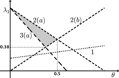
(b) First and Second-Step Bandwidths

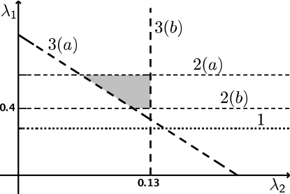
Notes: The diagram shows the rate conditions of Theorem 2 applied to the case where $h_{1j}=n^{-\lambda_{1}}$ for all $j$, $h_{2}=n^{-\lambda_{2}}$, and $K=n^{\theta}$. Condition 1, that is $\left(Kn\overline{h}_{1}\right)^{1/2}\overline{h}_{1}^{\rho_{1}+1}=O(1)$, is equivalent to $\lambda_{1}\geq(1+\theta)/(3+2\rho_{1})$; condition 2(a): ${K^{1/2}\log n}/{\left(n\overline{h}_{1}\right)^{1/2}}=o(1)$ $\Leftrightarrow$ $\lambda_{1}<1-\theta$; condition 2(b): $K\overline{h}_{1}=O(1)$ $\Leftrightarrow$ $\lambda_{1}\geq\theta$; condition 3(a): $\left(Kn\overline{h}_{1}\right)^{1/2}h_{2}^{\rho_{2}+1}=O(1)$ $\Leftrightarrow$ $\lambda_{1}\geq 1+\theta-2\lambda_{2}(\rho_{2}+1)$; and condition 3(b): $1/Kh_{2}^{3}=O(1)$ $\Leftrightarrow$ $\lambda_{2}\leq\theta/3$. Panel (a) illustrates the rate conditions on the first-step bandwidth and number of cutoffs $(\lambda_{1},\theta)$ for $\rho_{1}=1$, $\rho_{2}=3$, and $\lambda_{2}=\theta/3$, so that $h_{2}=K^{-1/3}$ and condition 3(b) is satisfied. Panel (b) displays the rate conditions on the bandwidths $(\lambda_{1},\lambda_{2})$ given $\theta=0.4$, $\rho_{1}=1$, and $\rho_{2}=3$.

Implementation of Theorem 2 requires the researcher to choose $\rho_{1}\in\mathbb{Z}_{+}$, $h_{1j}>0~{}\forall j$, $\rho_{2}\in\mathbb{Z}_{+}$, $h_{2}>0$, and $k(\cdot)$. A theory of optimal choice of these tuning parameters is beyond the goals of this paper. Optimal choice of bandwidths is an interesting topic for future research, because optimality in the multi-cutoff case would account for: (i) the interaction between first and second-stage bandwidths; (ii) the variance reduction from overlapping estimation windows at consecutive cutoffs; and (iii) the recent advances of robust bias-corrected inference and coverage-error optimal bandwidths by Calonico et al. (2018).

The IK bandwidth formula may produce first-step bandwidths with an incorrect rate of convergence. For example, if $\rho_{1}=1$, these bandwidths converge to zero at $n^{-0.2}$, which is not fast enough if $\rho_{2}=3$ (Figure 1). A simple way to correct for this is to adjust the bandwidths by multiplying them by $n^{0.2-\lambda_{1}}$ for $\lambda_{1}\geq\theta$, so that their rate becomes $n^{-\lambda_{1}}$. Conditions 2(a) and (b) imply that $\theta$ is never bigger than $0.5$ regardless of $\rho_{1}$, $\rho_{2}$, and $\lambda_{2}$. Thus, the smallest value for $\lambda_{1}$ consistent with these restrictions is $0.5$. The same idea applies to the coverage-error optimal bandwidths by Calonico et al. (2018), which converge to zero at rate $n^{-0.25}$, and need to be adjusted.

In certain cases, the $\beta$ function may depend on less than the three arguments $(c,d,d^{\prime})$. For example, in the Medicaid application, the treatment is binary and $\beta$ is only a function of $c$. This is a particular case of the theory in this section. The only rate condition that changes is condition 3(b). It becomes $1/Kh_{2}=O(1)$, or $\lambda_{2}\leq\theta$ in terms of Figure 1. A non-empty feasible set of bandwidth choices requires $\rho_{2}\geq 1$, as opposed to $\rho_{2}\geq 3$ in the general case.

A simple recommendation to implement Theorem 2 is to use the edge kernel, first-step rate-adjusted IK bandwidths for each cutoff, and a second-step bandwidth $h_{2}$ that minimizes the MSE of estimation. First, use observations pertaining to each cutoff $j$, compute the IK bandwidth $h_{1j}^{ik}$ for sharp RD and local-linear regression; adjust the rate of the bandwidths so that $h_{1j}=h_{1j}^{ik}\times n^{-0.3}$. Second, create a grid of possible values for $h_{2}$. For each value on the grid, compute $\widehat{\mu}^{c}(h_{2})$ using the edge kernel, the choices of $h_{1j}$ given above, $\rho_{1}=1$, and $\rho_{2}=3$ (or $\rho_{2}=1$ in the binary treatment case). Similarly, compute $\widehat{\mu}^{c^{\prime}}(h_{2})$ using the edge kernel, the choices of $h_{1j}$ given above, $\rho_{1}=2$, and $\rho_{2}=4$ (or $\rho_{2}=2$ in the binary treatment case). Use Equation 30 to estimate the variance of $\widehat{\mu}^{c}(h_{2})$ and call it $\widehat{\mathcal{V}}_{n}^{c}(h_{2})$. Evaluate the approximated MSE of $\widehat{\mu}^{c}(h_{2})$ by $(\widehat{\mu}^{c}(h_{2})-\widehat{\mu}^{c^{\prime}}(h_{2}))^{2}+\widehat{\mathcal{V}}_{n}^{c}(h_{2})$. Choose the bandwidth value on the grid that minimizes the MSE and call it $h_{2}^{*}$. The bias-corrected estimate is $\widehat{\mu}^{c^{\prime}}(h_{2}^{*})$, and its variance estimate is $\widehat{\mathcal{V}}_{n}^{c^{\prime}}(h_{2}^{*})$.

It may not be immediately clear that root-$n$ is the fastest estimation rate achievable in a setting where both $K$ and $n$ grow large. The double asymptotic setting is conceptually different from the usual asymptotic setting where only $n\to\infty$ and non-parametric averages are estimable at root-$n$. Estimation rates depend not only on bandwidth choices, but also on how fast $K$ grows, relative to $n$. Similar examples in econometrics include panels with a large number of observations and time periods, and asymptotics with many instruments. The following theorem demonstrates that the minimax optimal rate of estimation of $\mu^{c}$ is indeed root-$n$, as long as first-step bandwidths converge to zero at $1/K$ rate.

Theorem 3.

Let $\mathcal{P}$ be the class of models generating potential outcomes $\{Y_{i}(d)\}_{d\in\mathcal{D}}$ and forcing variables $X_{i}$. For a schedule of cutoffs and doses, $\{\bm{\mathrm{c}}_{j}\}_{j=1}^{K}$, observed data $(Y_{i},X_{i},D_{i})$ are generated iid from $P\in\mathcal{P}$ as described in Section 3.1. Assume that (i) each model $P\in\mathcal{P}$ satisfies Assumptions LABEL:assu_srd_est_fx-LABEL:assu_srd_kinf_est_int; (ii) $f(x)$ and $\sigma^{2}(x,d)$ are bounded away from zero uniformly in $\mathcal{P}$; (iii) the following functions are bounded uniformly in $\mathcal{P}$: $\nabla_{x}^{\rho}\sigma^{2}(x,d)~{}~{}\forall\rho\leq 1$ , $\nabla_{x}^{\rho}f(x)~{}~{}\forall\rho\leq 1$, $\nabla_{x}^{\rho}R(x,d)~{}~{}\forall\rho\leq\bar{\rho}$, $\nabla_{d}^{\rho}R(x,d)~{}~{}\forall\rho\leq\bar{\rho}$, where $\bar{\rho}=\max\{\rho_{1}+2,\rho_{2}+2\}$; and (iv) there exists $M\in(0,\infty)$ such that $\mathbb{P}[|Y_{i}(d)-R(X_{i},d)|<M]=1~{}~{}\forall d\in\mathcal{D}$ uniformly in $\mathcal{P}$. Then, for any $\epsilon>0$, there exists $\eta>0$ such that

$$\inf_{\widetilde{\mu}}\sup_{P\in\mathcal{P}}\mathbb{P}_{P}\left[\sqrt{n}|\widetilde{\mu}-\mu^{c}(P)|>\epsilon/2\right]\geq\frac{1}{4\eta}~{}\text{ for large }n.$$ (31)

The inf is taken over all estimators $\widetilde{\mu}$ built using the observed data $(Y_{i},X_{i},D_{i})$, $i=1,\ldots,n$; $\mu^{c}(P)=\int\omega^{c}(\bm{\mathrm{c}})\beta(\bm{\mathrm{c}};P)~{}d\bm{\mathrm{c}}$ with $\beta(\bm{\mathrm{c}};P)=\mathbb{E}_{P}[Y_{i}(d^{\prime})-Y_{i}(d)|X_{i}=c]$; and $\mathbb{P}_{P}$ and $\mathbb{E}_{P}$ denote the probability and expectation under model $P\in\mathcal{P}$.

Assume the conditions of Theorem 2, and that first-step bandwidths satisfy $\overline{h}_{1}=O(K^{-1})$. Consider the estimator $\widehat{\mu}^{c}$ defined in Equation 21. For any small $\delta>0$, there exists large $\epsilon\in(0,\infty)$ such that

$$\sup_{P\in\mathcal{P}}\mathbb{P}_{P}\left[\sqrt{n}|\widehat{\mu}^{c}-\mu^{c}(P)|>\epsilon\right]<\delta~{}\text{ for large }n.$$ (32)

Equation 31 shows that no estimator converges faster than $\sqrt{n}$ uniformly over $\mathcal{P}$. Equation 32 says the estimator proposed in Theorem 2 converges at root-$n$ uniformly over $\mathcal{P}$ as long as first-step bandwidths converge to zero at $1/K$ rate. Therefore, root-$n$ is the minimax optimal rate of convergence in the non-parametric estimation of ATE in RDD with many thresholds. Authors have previously analyzed minimax optimality of non-parametric estimators of a regression function at a boundary point, for example, Cheng et al. (1997) and Sun (2005). Theorem 3 is novel because it combines boundary points to estimate averages of non-parametric regression functions.

4 Fuzzy Case with Multiple Cutoffs

This section relaxes the sharp assignment mechanism of previous sections and studies the fuzzy RDD case. The analysis focuses on multiple cutoffs, but $K$ is finite as opposed to approaching infinity as in Section 3.2. This makes the exercise more tractable, because the number of compliance cases grows super-exponentially with the number of cutoffs. In contrast to the sharp case, non-parametric identification of local effects in the fuzzy case is impossible. As a result, inference methods in this section rely on a second heterogeneity assumption, namely, the treatment effect function is assumed parametric. Section B.5.2, in the supplemental appendix, provides practical guidelines to compute an MSE-optimal ATE estimator, and demonstrates asymptotic normality.

In the sharp RDD case, all individuals with forcing variable equal to $x$ receive the same treatment $D(x)$ (Equation 7). In the fuzzy RDD case, many of these individuals may receive treatments different from $D(x)$. In the high school assignment example, students may choose to go to a school that is not the best school for which they are eligible. For instance, a student may want to attend the same high school as a certain friend or sibling. Another example is given by Garibaldi et al. (2012). In their study, a schedule of tuition subsidies applies to most students at Bocconi University, but the university reserves the right to grant certain students different subsidies after reassessing their ability to pay.

The fuzzy RDD case is modeled in terms of a potential treatment assignment framework. A potential treatment assignment function $\mathcal{U}:\mathcal{X}\to\mathcal{D}$ describes the treatment received for every value of the forcing variable $x\in\mathcal{X}$. For simplicity, these functions are assumed to belong to the following class:

$$\mathcal{U}^{*}=\Bigg{\{}\mathcal{U}:\mathcal{X}\to\mathcal{D}~{}:~{}\mathcal{U}(x)=\sum\limits_{j=0}^{K}u_{j}\mathbb{I}\left\{c_{j}\leq x<c_{j+1}\right\}$$

$$\hskip 28.45274pt\text{ for some }u_{j}\in\{d_{0},\ldots,d_{K}\},j=0,\ldots,K\Bigg{\}}.$$ (33)

Sharp RDD is the particular case where the individual potential treatment assignment function $\mathcal{U}_{i}$ is the same for every individual $i$, that is, $\mathcal{U}_{i}(x)=D(x)~{}\forall i$ with $D(x)$ defined in Equation 7. In the fuzzy case, $\mathcal{U}_{i}$ is sampled iid from a distribution of functions with support in $\mathcal{U}^{*}$. Potential treatment functions $\mathcal{U}_{i}(x)$ are unobserved, but the treatments received are observed and given by

$$D_{i}=\sum\limits_{j=0}^{K}\mathcal{U}_{i}(c_{j})\mathbb{I}\left\{c_{j}\leq X_{i}<c_{j+1}\right\}.$$

Using classic definitions of compliance behaviors (Imbens and Rubin (1997)), three types of compliance groups are defined in terms of changes in treatment eligibility. “Never-changers” are those whose treatment received never changes when eligibility changes. The treatment received by “ever-compliers” or “ever-defiers” changes at least once when eligibility changes. Ever-compliers are those whose treatment received changes if and only if it changes to the treatment dose for which they become eligible. Ever-defiers change to a treatment dose different from the one for which they become eligible. In the case of one cutoff and two treatments, the definition of ever-complier (ever-defier) is equivalent to the classic definition of complier (defier) of Imbens and Lemieux (2008).

The three compliance groups are measurable events that partition the population of individuals with $\mathbf{G}_{nc}$ denoting never-changers, $\mathbf{G}_{ec}$ ever-compliers, and $\mathbf{G}_{ed}$ ever-defiers.

$$\mathbf{G}_{nc}=\Big{\{}\mathcal{U}_{i}\in\mathcal{U}^{*}:\left\{j:~{}\mathcal{U}_{i}(c_{j-1})\neq\mathcal{U}_{i}(c_{j})\right\}=\emptyset\Big{\}}$$ (34)

$$\mathbf{G}_{ec}=\Big{\{}\mathcal{U}_{i}\in\mathcal{U}^{*}:\left\{j:~{}\mathcal{U}_{i}(c_{j})=D(c_{j})\right\}\supseteq\left\{j:~{}\mathcal{U}_{i}(c_{j-1})\neq\mathcal{U}_{i}(c_{j})\right\}\neq\emptyset\Big{\}}$$ (35)

$$\mathbf{G}_{ed}=\Big{\{}\mathcal{U}_{i}\in\mathcal{U}^{*}:\left\{~{}\left\{j:~{}\mathcal{U}_{i}(c_{j})\neq D(c_{j})\right\}\cap\left\{j:~{}\mathcal{U}_{i}(c_{j-1})\neq\mathcal{U}_{i}(c_{j})\right\}~{}\right\}\neq\emptyset\Big{\}}$$ (36)

where $\emptyset$ denotes empty set.

In the high school assignment case, an example of a never-changer is a student who strongly prefers the high school with the lowest admission cutoff and attends that high school even if she is admitted to better schools. An example of an ever-complier is a student who attends the best school into which she is admitted, or a student who chooses the best school among the nearby schools. Suppose a student has rational preferences and is never indifferent. Assume her choice set is equal to those schools with admission cutoffs that are less than or equal to her test score. Then, such a student is never an ever-defier. In other words, as her test score increases, a new school is added to her choice-set of schools; she either chooses to go to the new school for which she becomes eligible, or she stays at the school which she preferred prior to the increase in her choice-set. Thus, it seems natural to rule out “ever-defiers” in this and other applications.

Never-changers do not produce changes in treatments, so there is no identification on them. For ever-compliers, there are multiple possible changes in treatment at a given cutoff, and ever-compliers may differ in terms of the treatments they comply with. For example, the student who is willing to attend the best school possible complies with all changes in treatment eligibility. On the other hand, the student who is willing to attend the best possible school within a certain distance from home only complies with some of the changes in treatment eligibility. Therefore, besides no-defiance, identification also requires the heterogeneity of ever-compliers to be restricted.

Assumption LABEL:assu_frd_id_nodef generalizes the sufficient conditions for identification on compliers in the one-cutoff case (Hahn et al. (2001) and Dong (2018a)). In addition, it restricts the heterogeneity on ever-compliers.

[assumptions.tex]assu00H

A fuzzy assignment produces several different treatment changes at each cutoff, even after ruling out ever-defiers. The researcher only observes one aggregate change in $Y_{i}$ at each cutoff, but there are several treatment effects on ever-compliers to be identified at that cutoff. Theorem 4 below shows that identification of these effects is not possible without further restricting the class of functions $\beta_{ec}(\bm{\mathrm{c}})$. Economic theory or a priori knowledge guides the choice of a functional form that credibly summarizes the heterogeneity of treatment effects. For example, the principal-agent model of Bajari et al. (2017) yields a functional form to study reimbursement of hospitals by insurers. The second heterogeneity assumption (Assumption LABEL:assu_srd_id_param) restricts the treatment effect function on ever-compliers to a finite-dimensional vector space of functions. [assumptions.tex]assu00G

In this case, the ATE on ever-compliers is a linear combination of the true parameter vector $\bm{\mathrm{\theta}}_{0}^{ec}$. For a counterfactual distribution $F$ chosen by the researcher,

$$\mu^{ec}(F)= \int\beta(\bm{\mathrm{c}};\bm{\mathrm{\theta}}_{0}^{ec})~{}dF(\bm{\mathrm{c}})$$ (37)

$$= \underset{\equiv\bm{\mathrm{Z}}(F)}{\underbrace{\int\left[\bm{\mathrm{\mathcal{W}}}(c,d^{\prime})-\bm{\mathrm{\mathcal{W}}}(c,d)\right]^{\prime}~{}dF(\bm{\mathrm{c}})}}\bm{\mathrm{\theta}}_{0}^{ec}$$ (38)

$$= \bm{\mathrm{Z}}(F)\bm{\mathrm{\theta}}_{0}^{ec}.$$ (39)

Theorem 4 shows that the observed change in average outcome at a given cutoff is a weighted average of treatment effects on ever-compliers who switch from various doses into the dose of eligibility at that cutoff. Assumption LABEL:assu_srd_id_param and variation in cutoff characteristics are sufficient conditions for identification. Conversely, identification on ever-compliers implies that $\beta_{ec}(\bm{\mathrm{c}})$ belongs to a finite-dimensional class of functions.

Theorem 4.

Under Assumption LABEL:assu_frd_id_nodef, for $j=1,\ldots,K$,

$$B_{j}=\sum\limits_{l=0,l\neq j}^{K}\omega_{j,l}\beta_{ec}(c_{j},d_{l},d_{j})$$

where $B_{j}$ is defined in Equation 10, and

$$\omega_{j,l}=\lim_{e\downarrow 0}\left\{\mathbb{P}[D_{i}=d_{l}|X_{i}=c_{j}-e]-\mathbb{P}[D_{i}=d_{l}|X_{i}=c_{j}+e]\right\},$$

for $l=0,1,\ldots,K,l\neq j$.

Moreover, suppose $\beta_{ec}$ belongs to the class of functions $\mathcal{H}$ defined in Assumption LABEL:assu_srd_id_param with $q\leq K$. Define

$$\widetilde{W}_{j}=\sum_{l=0,l\neq j}^{K}\omega_{j,l}\left[\bm{\mathrm{\mathcal{W}}}(c_{j},d_{j})-\bm{\mathrm{\mathcal{W}}}(c_{j},d_{l})\right]$$ (40)

for the vector-valued function $\bm{\mathrm{\mathcal{W}}}(c,d)$ of Assumption LABEL:assu_srd_id_param; build a $K\times q$ matrix $\widetilde{\bm{\mathrm{W}}}$ by stacking $\widetilde{W}_{j}$, and $\bm{\mathrm{B}}$ by stacking $B_{j}$. If $\widetilde{\bm{\mathrm{W}}}^{\prime}\widetilde{\bm{\mathrm{W}}}$ is invertible, then $\beta_{ec}(\bm{\mathrm{c}})$ is identified and equal to

$$\beta_{ec}(\bm{\mathrm{c}})=\left[\bm{\mathrm{\mathcal{W}}}(c,d^{\prime})-\bm{\mathrm{\mathcal{W}}}(c,d)\right]^{\prime}\left(\widetilde{\bm{\mathrm{W}}}^{\prime}\widetilde{\bm{\mathrm{W}}}\right)^{-1}\widetilde{\bm{\mathrm{W}}}^{\prime}\bm{\mathrm{B}}.$$

Conversely, suppose $\beta_{ec}$ belongs to some class of functions $\widetilde{\mathcal{H}}$, and treatment effects on ever-compliers are identified at the $p>K$ cutoff-dose values $\{\tilde{\bm{\mathrm{c}}}:\tilde{\bm{\mathrm{c}}}=(c_{j},d_{l},d_{j})\text{ with }\omega_{j,l}>0\}$ of every possible fuzzy assignment generated from the given schedule of cutoffs $\{\bm{\mathrm{c}}_{j}\}_{j=1}^{K}$. Then, the class of functions $\widetilde{\mathcal{H}}$ is “finite dimensional” in the sense that

$$\mathcal{G}=\Big{\{}\Big{(}\beta(\tilde{\bm{\mathrm{c}}}_{1}),\ldots,\beta(\tilde{\bm{\mathrm{c}}}_{p})\Big{)}:\text{ for }\beta\in\widetilde{\mathcal{H}}\Big{\}}\subseteq\mathbb{R}^{p}$$

has $dim\mathcal{G}\leq K$ for every fuzzy assignment $\{\tilde{\bm{\mathrm{c}}}_{j}\}_{j=1}^{p}$ generated from $\{\bm{\mathrm{c}}_{j}\}_{j=1}^{K}$.

Theorem 4 reveals the requirement of stronger functional form assumptions on $\beta_{ec}(\bm{\mathrm{c}})$ even for identification of local effects in the fuzzy case with a finite number of multiple cutoffs. For example, identification is not possible when $\widetilde{\mathcal{H}}$ is the class of all smooth functions studied in the non-parametric case of Section 3.2. The result is striking because non-parametric identification of local effects is possible both in the sharp case with a finite number of cutoffs and in the fuzzy case with a single cutoff. It is likely possible to obtain non-parametric identification of $\beta_{ec}(\bm{\mathrm{c}})$ under a large variation of cutoff-dose values. The function $\beta_{ec}(\bm{\mathrm{c}})$ may be approximated by a sequence of parametric functions from Assumption LABEL:assu_srd_id_param, where $q$ grows to infinity more slowly than $K$, so to keep $dim\mathcal{G}\leq K$ as $K\to\infty$. In this paper, the number of cutoffs is kept finite for simplicity, and the case with large $K$ is deferred to future work.

Theorem 4 also clarifies the interpretation of two-stage least squares (2SLS) estimates in applications of fuzzy RD with multiple cutoffs, a common practice in applied work. The practice consists of using $D(X_{i})$ as an instrument for $D_{i}$ in the regression of $Y_{i}$ on a constant, $D_{i}$, and $X_{i}$. See Angrist and Pischke (2008) for a discussion. In the single-cutoff case, both the non-parametric RD estimator and 2SLS applied to a neighborhood of the cutoff are consistent to the average treatment effect on compliers (Hahn et al. (2001)). To my knowledge, such an equivalence has never been studied in the multiple-cutoff case. Nevertheless, many important applications have multiple-fuzzy cutoffs and use 2SLS; for example, Angrist and Lavy (1999), Chen and Van der Klaauw (2008), and Hoekstra (2009). The 2SLS estimator is consistent for a data-driven weighted average of treatment effects on ever-compliers as long as a sufficiently flexible specification is used; for example, cutoff fixed-effects or varying slopes. The economic meaning of the 2SLS estimands depends crucially on the choice of such a weighting scheme. Unless a parametric functional form is imposed on $\beta_{ec}(\bm{\mathrm{c}})$, or there is large variation in cutoff-doses, only a data-driven weighted average of $\beta_{ec}(\bm{\mathrm{c}})$ is identified. In other words, if $\beta_{ec}(\bm{\mathrm{c}})$ is non-parametric and there are only a few cutoffs, the researcher does not have control over the weighting scheme, and 2SLS estimates don’t have a clear interpretation.

Theorem 4 leads to a two-step estimation procedure for $\bm{\mathrm{\theta}}^{ec}_{0}$ and $\mu^{ec}$. The mechanics are similar to the previous sections, so I omit the details from the main text for brevity. In the first step, the researcher estimates the jump discontinuity of the vector $[Y_{i}~{}~{}\bm{\mathrm{\mathcal{W}}}(X_{i},D_{i})^{\prime}]^{\prime}$ using LPRs at each cutoff to obtain $[\widehat{B}_{j}~{}~{}\widehat{\widetilde{W}}_{j}^{\prime}]^{\prime}$. In the second step, a regression of $\widehat{B}_{j}$ on $\widehat{\widetilde{\bm{\mathrm{W}}}}_{j}^{\prime}$ obtains $\widehat{\bm{\mathrm{\theta}}}^{ec}$. The ATE estimator is $\widehat{\mu}^{ec}=\bm{\mathrm{Z}}(F)\widehat{\bm{\mathrm{\theta}}}^{ec}$. Estimation precision varies across cutoffs, and the parametric form of $\beta_{ec}$ allows us to optimally combine different cutoffs to minimize the MSE of $\widehat{\bm{\mathrm{\theta}}}^{ec}$. The researcher can simply re-weight the second-step regression by the inverse of the MSE matrix of the first-step estimators. Section B.5.2 in the supplemental appendix delineates the estimation and inference procedures of $\bm{\mathrm{\theta}}^{ec}_{0}$ and $\mu^{ec}$ with practical steps.

5 Simulations

In this section, Monte Carlo simulations illustrate the finite sample behavior of the ATE estimator proposed in Section 3.2. The analysis considers estimation precision and coverage of confidence intervals for different choices of tuning parameters and a non-linear specification for $\beta$. As predicted by Theorem 2, an incorrect choice of the second-step polynomial degree leads to severe bias and extremely poor coverage of confidence intervals. Moreover, first-step bandwidths that imply overlapping estimation windows produce lower MSE than cases with no overlap, regardless of other tuning parameters.

The DGP draws $n$ iid observations of $(X_{i},\varepsilon_{i})$ where $X_{i}$ is uniformly distributed over $[0,1]$, $\varepsilon_{i}$ is normally distributed with zero mean and unit variance, and these variables are independent of each other. There are $K$ cutoffs $c_{j}=j/(K+1)$, $j=1,\ldots,K$, on the unit interval $[0,1]$. The number of cutoffs is $K=\lfloor n^{0.4}\rfloor$, where $\lfloor a\rfloor$ denotes the largest integer smaller than or equal to $a$. An individual with forcing variable $X_{i}$ receives a treatment dose equal to $D(X_{i})$ as in Equation 7. The dose increases by one unit at each cutoff, starting at $d_{0}=1$ and ending at $d_{K}=K+1$. The outcome variable is $Y_{i}=\phi(X_{i})D(X_{i})+\varepsilon_{i}$ where $\phi(X_{i})=15X_{i}^{3}+7.5X_{i}^{2}-18.75X_{i}+2.125$. This implies that $\beta(\bm{\mathrm{c}})=\phi(c)(d^{\prime}-d)$, which falls into the binary treatment case (see discussion on page 3.2). Consider a counterfactual policy that uniformly increases treatment doses by one unit. The ATE parameter $\mu$ is the integral of $\phi(c)$ over $c\in[0,1]$, which equals $-1$ in this case.

Estimation follows the procedure suggested in Section 3.2. For given bandwidth choices $h_{1}$ and $h_{2}$, I compare the ATE estimator $\widehat{\mu}$ that uses $\rho_{1}=\rho_{2}=1$, to the bias-corrected ATE estimator $\widehat{\mu}^{bc}$ that uses $\rho_{1}=\rho_{2}=2$. To emphasize the importance of the second step, I also compute a naive ATE estimator that simply averages the first-step estimates. The naive and bias-corrected naive estimators, respectively $\widetilde{\mu}$ and $\widetilde{\mu}^{bc}$, are constructed as $\widehat{\mu}$ and $\widehat{\mu}^{bc}$ except for the tuning parameters in the second step. Both naive estimators use $\rho_{2}=0$ and $h_{2}=\infty$. To examine the effect of overlapping estimation windows in the first step, I compare estimators for two choices of $h_{1}$. The first choice is the largest possible bandwidth $h_{1}=1/(K+1)$, which leads to maximum overlap. The second choice is the largest possible bandwidth with no overlap, that is, $h_{1}=0.5/(K+1)$. Finally, I study the effects of ten different choices for the second-step bandwidth, $h_{2}\in\{3/(K+1),\ldots,12/(K+1)\}$. All choices of tuning parameters satisfy the rate conditions of Theorem 2 and produce a convergence rate of root-$n$ for $\widehat{\mu}$ and $\widehat{\mu}^{bc}$. The Monte Carlo experiment simulates 10,000 draws of an iid sample with $n\in\{1789,10120,27886,57244,100000\}$ and $K\in\{20,40,60,80,100\}$, respectively. Section B.7 in the supplemental appendix repeats the experiment with data-driven bandwidth choices, following the bandwidth rules proposed on page 3.2 (Section 3.2).

Table 1: Precision of Estimators - Choice of $h_{1}$

Notes: The table reports simulated bias, variance, and mean squared error (MSE) for four estimators $(\widehat{\mu},\widehat{\mu}^{bc},\widetilde{\mu},\widetilde{\mu}^{bc})$, two choices of first-step bandwidth (overlap and no overlap), and five sample sizes $n$ and respective numbers of cutoffs $K$. The second-step bandwidth is set to $h_{2}=3/(K+1)$, which minimizes MSE of $\widehat{\mu}$. Refer to Table 2 for different choices of $h_{2}$. The number of simulations is 10,000.

The bias and variance of all estimators converge to zero as the sample size increases, regardless of the choice of $h_{1}$ (Table 1). The bias-correction of $\widehat{\mu}^{bc}$ eliminates almost all the bias of $\widehat{\mu}$, at the cost of a higher variance. The naive estimator $\widetilde{\mu}$ oversmooths the second step beyond the conditions of Theorem 2. As a result, the bias of $\widetilde{\mu}$ is substantially larger than that of $\widehat{\mu}$. Simply correcting for bias in the first step does not solve the problem, as the difference in bias between $\widetilde{\mu}$ and $\widetilde{\mu}^{bc}$ is small. First-step bandwidths that produce overlap (Table 1, rows 1-5) yield approximately the same bias, but substantially smaller variance, compared to first-step bandwidths that produce no overlap (Table 1, rows 6-10).

Table 2: Precision of Estimators - Choice of $h_{2}$

Notes: The table reports simulated bias, variance, and mean squared error (MSE) for two estimators $(\widehat{\mu},\widehat{\mu}^{bc})$, ten choices of second-step bandwidth ($h_{2}\in\{3/(K+1),\ldots,12/(K+1)\})$, and the two smallest sample sizes $n$ and respective numbers of cutoffs $K$. The first-step bandwidth is set to $h_{1}=1/(K+1)$ (overlap). Naive estimators $(\widetilde{\mu},\widetilde{\mu}^{bc})$ are not in this table because they are not affected by the choice of $h_{2}$. The number of simulations is 10,000.

Next, I study how the choice of $h_{2}$ affects precision of $(\widehat{\mu},\widehat{\mu}^{bc})$ for a fixed choice of $h_{1}=1/(K+1)$ (Table 2). The smallest value for $h_{2}$ is $3/(K+1)$. This defines a second-step estimation window with at least three cutoffs to ensure invertibility of matrices in the regressions. The bias of $\widehat{\mu}$ is substantially smaller when $h_{2}$ is set to its smallest value. All other measures are practically unaffected across different $h_{2}$.

The significant bias of the naive ATE estimators $\widetilde{\mu}$ and $\widetilde{\mu}^{bc}$ decreases the coverage of 95% confidence intervals as the sample increases (Table 3). The naive estimators oversmooth in the second step, and Theorem 2 implies the bias grows faster than root-$n$. For each of the four estimators, the confidence intervals equal the estimator plus or minus $1.96$ times its standard error. The variance of estimators are obtained as described in Equation 30. The bias-corrected ATE estimator $\widehat{\mu}^{bc}$ produces confidence intervals with correct coverage for all samples sizes. Although $\widehat{\mu}$ yields intervals with average length smaller than $\widehat{\mu}^{bc}$, the bias of $\widehat{\mu}$ leads to a slightly lower coverage.

Table 3: Coverage of 95% Confidence Intervals

Notes: The table reports simulated percentage of correct coverage and average length of 95% confidence intervals. Confidence intervals are constructed using four estimators $(\widehat{\mu},\widehat{\mu}^{bc},\widetilde{\mu},\widetilde{\mu}^{bc})$. They equal an estimator plus or minus its estimated standard deviation multiplied by $1.96$. Coverage and average length are computed for five sample sizes $n$ and respective numbers of cutoffs $K$. The first-step bandwidth is set to $h_{1}=1/(K+1)$ (overlap), and the second-step bandwidth is set to $h_{2}=3/(K+1)$, which minimizes MSE of $\widehat{\mu}$. The number of simulations is 10,000.

6 Application

In this section, the methods proposed in this paper are illustrated using the data from PU on high school assignments in Romania. Many policy questions demand an ATE of a continuous counterfactual distribution of treatments, and this section provides an example of such a policy question. The estimators designed for the sharp RDD case are consistent for “Intent-to-Treat” (ITT) average effects when applied to the fuzzy data of PU. In this application, the ITT effect measures the impact of being assigned to a better school but not necessarily attending it. The parametric methods of Section 4 yield noticeable efficiency gains in the estimation of the ATE on ever-compliers. Treatment effects for ever-compliers reveal a heterogeneity pattern unlike the heterogeneity of ITT effects.

The administrative data from Romania cover 3 cohorts of 9th grade students for the years 2001, 2002, and 2003, with a total of 334,137 observations. The essential elements of the high school assignment in Romania are described below. The assignment to high school is nationally centralized by the Ministry of Education. At the end of grade 8, students submit a transition score and a complete ranking of preferences for high schools. The transition score is an average of the student’s performance on a national exam taken in grade 8 and the student’s grade point average during grades 5-8. The Ministry of Education ranks students by their transition score and no other criteria. The mechanism assigns the student ranked first to her most preferred school, the student ranked second to her most preferred school, etc. Students cannot decline their assignment, and they have incentives to truthfully reveal their preference rankings.

The observed variables are the town and year of student $i$, the transition score $X_{i}$, the school the student is assigned to, and the student’s score on the “baccalaureate exam.” This is an exam taken at the end of high school, and the grade on the exam is the outcome variable $Y_{i}$. The quality of school $j$ (treatment dose $d_{j}$) is measured by the average transition score of the students attending that school $j$. The cutoff $c_{j}$ for admission into a school $j$ is equal to the minimum transition score among the students that are assigned to that school $j$. The student’s preferences in high schools are not observed in the data, which makes the RDD fuzzy. For example, a student may have a score greater than the cutoff for the best school in her town, but still be assigned to a different school because of her personal preferences. For a transition score $X_{i}$, the treatment dose of eligibility $D(X_{i})$ is equal to the largest $d$ among those schools with admission cutoff $c$ less than $X_{i}$. The treatment dose received $D_{i}$ coincides with the treatment dose of eligibility $D(X_{i})$ for 40% of the students in the sample. Thus, the assignment is fuzzy, and causal inference beyond ITT effects requires the methods of Section 4. Following PU, I drop observations with missing values for $Y_{i}$. I also drop cutoffs without enough observations around them to carry out the matrix inversions of the local polynomial regressions. The dropping of cutoffs leaves the empirical distribution of outcomes, forcing variable, cutoffs, and treatment doses practically unchanged. The estimation sample has 588 cutoffs with a total of 179,995 individuals from 769 schools in 121 towns and 3 years. The variation of cutoff and dose values is displayed in Figure 2.

Figure 2: Variation in Cutoff and Dose Values

(a)

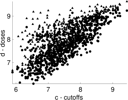
(b)

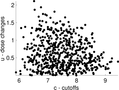
Notes: Scatter plot with cutoff values on the x-axis and dose values on the y-axis for the $K=588$ cutoffs in the Romanian data. Panel (a) shows both doses before and after the cutoff, that is, $d_{j-1}$ in black and $d_{j}$ in gray. Panel (b) displays dose-change values on the y-axis, that is, $u_{j}=d_{j}-d_{j-1}$. The peer-quality of school $j$ (treatment dose $d_{j}$) is measured by the average transition score of the students attending that school $j$. The cutoff $c_{j}$ for admission into a school $j$ is equal to the minimum transition score among the students assigned to school $j$.

Non-parametric identification of $\beta(\bm{\mathrm{c}})$ is limited to the set $\mathcal{C}$, which is the convex-hull of $\mathcal{C}_{\infty}$. The set $\mathcal{C}_{\infty}$ is not entirely observed, and the researcher relies on the observation of $\mathcal{C}_{K}$ (Figure 2(a)). For the sake of simplicity, I restrict $\beta$ to be a function of dose changes ($u=d^{\prime}-d$) instead of doses before and after ($d$ and $d^{\prime}$). The restriction greatly simplifies the visualization and estimation of $\beta(c,d,d^{\prime})$, because it implies that $\beta(c,d,d^{\prime})=\phi(c)(d^{\prime}-d)$, where $\phi$ is a continuously differentiable function. Figure 2(b) illustrates the variation of cutoff and dose-change values and defines the limits on identification of policy counterfactuals. For example, it is not possible to identify the effects of randomly assigning students with grades between 8 and 9 to a change in treatment dose of 2. The support of such counterfactual distribution falls outside the observed variation of cutoff and dose-change values. On the other hand, it is possible to identify the ATE of randomly assigning students with grades between 6.5 and 8.5 to dose increases between 0 and 1.5.

The following policy question illustrates the ATE estimator proposed in this paper. Suppose a new charter school is constructed in one of the towns in Romania. The new charter school has more autonomy and better management than traditional public schools, and admitted students experience an increase in school quality as if they were admitted to a school with better peers. More specifically, the policy counterfactual is to give a 0.5 increase in peer-quality to a uniform distribution of scores between 6.5 and 8.5. The ATE parameter is defined as

$$\mu=\frac{1}{2}\bigintssss_{6.5}^{8.5}\phi(c)~{}dc.$$ (41)

I follow the estimation procedure suggested in Section 3.2 and take into account the restriction $\beta(c,d,d^{\prime})=\phi(c)(d^{\prime}-d)$. As in the binary treatment case, the restriction lowers the polynomial degree requirement on the second-step estimation to $\rho_{2}=1$. See Figure 1 and the discussion that follows it. The grid for $h_{2}$ has 32 equally-spaced points between 0.1 and 3.6, respectively, the smallest bandwidth for which the estimator is computable, and the maximum distance between two different cutoffs. The MSE-optimal bandwidth choice is $h_{2}^{*}=1.837$. The new charter school has a bias-corrected ATE of $0.2964$ with standard error of $0.1296$, and it is statistically significant at 5%. Figure 3(a) plots $0.5\widehat{\phi}(c)$, that is, the effect of a $0.5$ increase in the treatment dose for various levels of $c$. The graph reveals heterogeneous marginal effects of ability on returns to school quality. Heterogeneity of treatment effects is a priori unknown, and the ATE estimator proposed in this paper is consistent for $\mu$ regardless of the shape of $\phi(c)$. This highlights the empirical relevance of Theorem 2 and the importance of the second-step estimation. In other words, the common strategy of normalizing all cutoffs to zero and estimating one discontinuity using the pooled data is not consistent for $\mu$ when $\phi(c)$ has such heterogeneity.

Figure 3: Treatment Effect Function

(a)

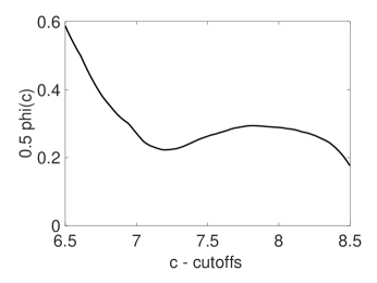
(b)

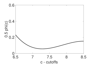
Notes: Estimated average treatment effect function for a $0.5$ increase in school quality for students with score equal to $c$. The figure plots $\widehat{\beta}(c,d,d+0.5)=0.5\widehat{\phi}(c)$ for $c\in[6.5,8.5]$. Panel (a) shows the ITT effect of a 0.5 increase in average peer performance for various levels of transition score. The $\phi$ function is estimated non-parametrically with bias correction following Section 3.2 (sharp case). Panel (b) displays the effect on ever-compliers of the same uniform change in treatment dose. The $\phi$ function is estimated parametrically with bias correction following the iterated procedure of Section B.5.2 in the supplemental appendix (fuzzy case).

Estimation of treatment effects on ever-compliers requires a parametric functional form on $\beta_{ec}$ (Theorem 4). I assume $\beta_{ec}(c,d,d^{\prime})=\theta_{1}(d^{\prime}-d)+\theta_{2}c(d^{\prime}-d)+\theta_{3}c^{2}(d^{\prime}-d)+\theta_{4}c^{3}(d^{\prime}-d)$ and carry out the iterative estimation procedure described in the supplemental appendix’s Section B.5.2. The algorithm achieves convergence of $\theta$s within 30 iterations. The iterated bias-corrected ATE on ever-compliers equals $0.107$ with standard error of $0.0109$. The precision is substantially greater than the non-parametric case. Figure 3(b) displays the treatment effect function on ever-compliers for a dose change of $0.5$. Compared to ITT effects in Figure 3(a), the return of better schooling on ever-compliers is also positive, but much less heterogeneous across ability levels.

7 Conclusion

Difficulty in gathering experimental data in many fields within the social sciences makes quasi-experimental techniques such as RDD extremely important to evaluate policies and social programs. RDD has been used in a wide range of applications in economics since the late 1990s. More recently, there has been an increasing number of applications with one forcing variable and multiple cutoffs, assigning individuals to heterogeneous treatments. The demand for multi-cutoff RDD methods is constantly growing, as richer data sets become ever more available.

This paper states conditions under which multiple RDD effects are combined to infer ATE over the entire range of cutoff values. The proposed estimator is consistent and asymptotically normal for ATEs over the entire support of variation in cutoffs and treatment doses. Asymptotic results are derived under a large number of observations and cutoffs in the sharp case of non-parametric treatment effect functions. Sufficient conditions on the rate of growth of the number of cutoffs, relative to the number of observations, are given. These rate conditions determine the feasible choice set of tuning parameters. This paper also shows that non-parametric identification in fuzzy RDD with multiple cutoffs is impossible unless the treatment effect function is finite-dimensional, or there is large variation of cutoff-dose values. A parametric specification provides an MSE-optimal ATE estimator for the fuzzy case that is consistent and asymptotically normal.

The relevance of the ATE estimators proposed in this paper is illustrated with the data of Pop-Eleches and Urquiola (2013) on high school assignment in Romania. Of interest is the effect of high school quality on academic performance of students. I find strong evidence of non-linearities in the returns to better schooling, as a function of students’ ability level. Monte Carlo simulations demonstrate that such non-linearities severely bias a naive average of local effects that does not use the correction weighting scheme proposed in this paper. Applying the fuzzy RDD methods to the Romanian data reveals causal effects on ever-compliers that are smaller and less heterogeneous than ITT effects.

The proposed estimator converges at the minimax optimal rate of root-$n$, as long as first-step bandwidths converge to zero at $1/K$ rate. It would be interesting to learn about efficiency properties of the ATE estimator. Theoretical tools commonly employed to derive efficiency lower-bounds may not be immediately applicable to the setting of this paper. These tools are designed for regular estimators, and for data drawn from a population where the parameter of interest is identified. In contrast, the fixed-cutoff RDD design relies on an “identification at infinity argument”, and I wonder about the sufficient conditions that would obtain regularity of the ATE estimator. A possibility for future work is to the generalize the uniform convergence tools from this paper to arrive at such conditions.

8 Acknowledgements

I am indebted to Han Hong, Caroline Hoxby, and Guido Imbens for invaluable advice. The paper also benefited from feedback received from seminar participants at Stanford, Boston University, Cambridge, Iowa, Notre Dame, CORE-UcLouvain, UCSD, UCDavis, FGV-EESP, FGV-EPGE, Insper, PUC-Rio, Toulouse, UIUC, and at various conferences. I thank Tim Bresnahan, Arun Chandrasekhar, Michael Dinerstein, Ivan Fernandez-Val, Ivan Korolev, Michael Leung, Huiyu Li, Jessie Li, Petra Moser, Stephen Terry, Xiaowei Yu, and anonymous referees for suggestions and comments. I gratefully acknowledge the financial support received from the B.F. Haley and E.S. Shaw Fellowship at SIEPR-Stanford, CORE-UcLouvain, ISLA-Notre Dame, and while visiting the Kenneth C. Griffin Department of Economics at the University of Chicago.

Appendix A Appendix

Throughout the appendices, $M$ is used as a generic finite and positive constant in the proofs. For a $p\times q$ matrix A, the norm of A is induced by the Euclidean norm $\|\cdot\|$, i.e. $\|A\|=\max_{x\in\mathbb{R}^{q},x\neq 0}\|Ax\|/\|x\|$. The determinant of matrix $A$ is denoted $\det(A)$. References to the supplemental appendix include B in the numbering; for example, Lemma B.1, or Table B.2.

A.1 Proof of Theorem 1

Lemma B.1 derives asymptotic normality of the bias-corrected jump-discontinuity estimator at one cutoff based on local polynomial regressions of a vector $\bm{\mathrm{Y}}_{i}$ on a scalar forcing variable $X_{i}$. The proof of Theorem 1 is a straightforward generalization of Lemma B.1 in the particular case of a scalar $Y_{i}$. As the sample size increases and the number of cutoff remains fixed, the jump-discontinuity estimators are independent across cutoffs. First apply Lemma B.1 to each cutoff individually, and then aggregate over cutoffs.

$\square$

A.2 Proof of Lemma 2

Define $\overline{\mathcal{C}}=[\underline{\mathcal{X}},\overline{\mathcal{X}}]\times[\underline{\mathcal{D}},\overline{\mathcal{D}}]\times[\underline{\mathcal{D}},\overline{\mathcal{D}}]$. Consider the partition of $\overline{\mathcal{C}}$ made of the set of non-intersecting cubicles $T_{n}=\{C_{1},\ldots,C_{M}\}$ with $M=n^{3}$, $n=\{1,2,\ldots\}$. Each $C_{j}$ is a half-open cubicle of the form $[x_{l-1},x_{l})\times[y_{m-1},y_{m})\times[z_{o-1},z_{o})$ with sides of lengths equal to $(\overline{\mathcal{X}}-\underline{\mathcal{X}})/n$, $(\overline{\mathcal{D}}-\underline{\mathcal{D}})/n$, and $(\overline{\mathcal{D}}-\underline{\mathcal{D}})/n$. Define the sub-collection $U_{n}=\{C\in T_{n}:~{}C\subset\mathcal{C}\}=\{A_{1},\ldots,A_{Q}\}$. Since $\mathcal{C}_{\infty}$ is dense in $\mathcal{C}$, for every $A_{j}\in U_{n}$, find a point $\bm{\mathrm{c}}_{j}\in\mathcal{C}_{\infty}\cap A_{j}$ for which $\beta(\bm{\mathrm{c}}_{j})$ is known. The sum $\mu_{n}=\sum_{j=1}^{Q}\omega(\bm{\mathrm{c}}_{j})\beta(\bm{\mathrm{c}}_{j})\left(\overline{\mathcal{X}}-\underline{\mathcal{X}}\right)\left(\overline{\mathcal{D}}-\underline{\mathcal{D}}\right)^{2}/n^{3}$ converges to $\mu^{c}$ as $n\to\infty$ because $\omega(\bm{\mathrm{c}})\beta(\bm{\mathrm{c}})$ is Riemann integrable on $\mathcal{C}$.

$\square$

A.3 Proof of Theorem 2

The proof combines arguments from the proof of Lemma B.1 with lemmas on the uniform convergence of empirical processes from Sections B.2 and B.3. Define $\mu^{*}$, $\widetilde{\mu}$, and $\mu_{n}$ as follows:

$$\mu^{*}= \sum_{j=1}^{K}\Delta_{j}\Big{\{}e_{1}^{\prime}\mathbb{E}[G_{n}^{j+}]\frac{1}{nh_{1j}}\sum_{i=1}^{n}k\left(\frac{X_{i}-c_{j}}{h_{1j}}\right)v_{i}^{j+}Y_{i}\widetilde{H}_{i}^{j}$$

$$\hskip 34.14322pt-e_{1}^{\prime}\mathbb{E}[G_{n}^{j-}]\frac{1}{nh_{1j}}\sum_{i=1}^{n}k\left(\frac{X_{i}-c_{j}}{h_{1j}}\right)v_{i}^{j-}Y_{i}\widetilde{H}_{i}^{j}\Big{\}}$$ (A.1)

$$= \sum_{j=1}^{K}\Delta_{j}\frac{1}{nh_{1j}}\sum_{i=1}^{n}k\left(\frac{X_{i}-c_{j}}{h_{1j}}\right)Y_{i}e_{1}^{\prime}\left(v_{i}^{j+}\mathbb{E}[G_{n}^{j+}]-v_{i}^{j-}\mathbb{E}[G_{n}^{j-}]\right)\widetilde{H}_{i}^{j}$$ (A.2)

$$\widetilde{\mu}= \sum_{j=1}^{K}\Delta_{j}\left\{e_{1}^{\prime}G_{n}^{j+}\mathbb{E}\left[\frac{1}{nh_{1j}}\sum_{i=1}^{n}k\left(\frac{X_{i}-c_{j}}{h_{1j}}\right)v_{i}^{j+}Y_{i}^{j+}\widetilde{H}_{i}^{j}\right]\right.$$

$$\hskip 34.14322pt\left.-e_{1}^{\prime}G_{n}^{j-}\mathbb{E}\left[\frac{1}{nh_{1j}}\sum_{i=1}^{n}k\left(\frac{X_{i}-c_{j}}{h_{1j}}\right)v_{i}^{j-}Y_{i}^{j-}\widetilde{H}_{i}^{j}\right]\right\}$$

$$\mu_{n} =\sum_{j=1}^{K}\Delta_{j}B_{j}.$$ (A.3)

Write

$$\frac{\widehat{\mu}-\mathcal{B}_{1n}^{c}-\mathcal{B}_{2n}^{c}-\mu}{(\mathcal{V}_{n}^{c})^{1/2}}= \frac{\mu^{*}-\mathbb{E}[\mu^{*}|\mathcal{X}_{n}]}{(\mathcal{V}_{n}^{c})^{1/2}}$$ (A.4)

$$+ {\frac{\widetilde{\mu}-\mathcal{B}_{1n}^{c}}{(\mathcal{V}_{n}^{c})^{1/2}}}$$ (A.5)

$$+ \frac{\mu_{n}-\mathcal{B}_{2n}^{c}-\mu}{(\mathcal{V}_{n}^{c})^{1/2}}$$ (A.6)

$$+ \frac{\widehat{\mu}-\mathbb{E}[\widehat{\mu}|\mathcal{X}_{n}]-\left(\mu^{*}-\mathbb{E}[\mu^{*}|\mathcal{X}_{n}]\right)}{(\mathcal{V}_{n}^{c})^{1/2}}$$ (A.7)

$$+ \frac{\mathbb{E}[\widehat{\mu}-\mu_{n}|\mathcal{X}_{n}]-\widetilde{\mu}}{(\mathcal{V}_{n}^{c})^{1/2}}.$$ (A.8)

The proof in this appendix applies a central limit theorem (CLT) to show that Part (A.4) converges in distribution to a standard normal; it demonstrates that $\mathcal{B}_{1n}$ approximates the first-step bias, that is, that part (A.5) converges in probability to zero; and it shows that $\mathcal{B}_{2n}$ approximates the second-step bias (integration error), that is, that part (A.6) converges to zero. Lemma B.7 shows that parts (A.7) and (A.8) converge in probability to zero.

Part (A.4)

First, find the rate that $(\mathcal{V}_{n}^{c})^{-1/2}$ grows. Define $\phi_{n}$ and rewrite $\mathcal{V}_{n}^{c}$ as follows:

$$\phi_{n}(X_{i})= \sum_{j=1}^{K}\frac{\Delta_{j}}{nh_{1j}}k\left(\frac{X_{i}-c_{j}}{h_{1j}}\right)e_{1}^{\prime}\left(v_{i}^{j+}\mathbb{E}[G_{n}^{j+}]-v_{i}^{j-}\mathbb{E}[G_{n}^{j-}]\right)\widetilde{H}_{i}^{j}$$ (A.9)

$$\mathcal{V}_{n}^{c}= \sum_{i=1}^{n}\mathbb{E}\left[\varepsilon_{i}^{2}\phi_{n}(X_{i})^{2}\right].$$ (A.10)

Choose alternative bandwidths $h_{1j}^{*}$, $j=1,\ldots,K$, such that (i) there exists $\delta>0$ (independent of $n$) such that $\delta<h_{1j}^{*}/h_{1j}\leq 1~{}\forall j$ ; and (ii) $[c_{j}-h_{1j}^{*},c_{j}+h_{1j}^{*}]\cap[c_{j^{\prime}}-h_{1j^{\prime}}^{*},c_{j^{\prime}}+h_{1j^{\prime}}^{*}]=\emptyset$ for any $j\neq j^{\prime}$.

$$\mathcal{V}_{n}^{c} =n\mathbb{E}\left[\zeta^{2}(X_{i})\phi_{n}^{2}(X_{i})\right]\geq n\sum_{j=1}^{K}\bigintss_{c_{j}-h_{1j}^{*}}^{c_{j}+h_{1j}^{*}}\zeta^{2}(x)\phi_{n}^{2}(x)f(x)~{}dx$$ (A.11)

$$=n\sum_{j=1}^{K}\bigintss_{c_{j}-h_{1j}^{*}}^{c_{j}+h_{1j}^{*}}\zeta^{2}(x)\Bigg{(}\frac{\Delta_{j}}{nh_{1j}}k\left(\frac{x-c_{j}}{h_{1j}}\right)e_{1}^{\prime}\left(\mathbb{I}\{x\geq 0\}\mathbb{E}[G_{n}^{j+}]-\mathbb{I}\{x<0\}\mathbb{E}[G_{n}^{j-}]\right)$$

$$\hskip 128.0374ptH\left(\frac{x-c_{j}}{h_{1j}}\right)\Bigg{)}^{2}f(x)~{}dx$$ (A.12)

$$=\frac{1}{Kn}\frac{1}{K}\sum_{j=1}^{K}\frac{K^{2}\Delta_{j}^{2}}{h_{1j}}\bigintss_{-h_{1j}^{*}/h_{1j}}^{h_{1j}^{*}/h_{1j}}\zeta^{2}(c_{j}+uh_{1j})\Bigg{(}k\left(u\right)e_{1}^{\prime}\left(\mathbb{I}\{u\geq 0\}\mathbb{E}[G_{n}^{j+}]-\mathbb{I}\{u<0\}\mathbb{E}[G_{n}^{j-}]\right)$$

$$\hskip 221.93158ptH\left(u\right)\Bigg{)}^{2}f(c_{j}+uh_{1j})~{}du~{}\geq~{}\frac{M}{Kn\overline{h}_{1}}$$ (A.13)

where the first inequality follows from the integrand being positive and $\cup_{j=1}^{K}[c_{j}-h_{1j}^{*},c_{j}+h_{1j}^{*}]\subseteq\cup_{j=1}^{K}[c_{j}-h_{1j},c_{j}+h_{1j}]$; the third equality uses a change of variables $u=(x-c_{j})/h_{1j}$; and the last inequality follows because (a) $h_{1j}\leq\overline{h}_{1}$; (b) $K^{2}\Delta_{j}^{2}$ is bounded away from zero uniformly over $j$ (Lemma B.9); and (c) each integral is bounded away from zero over $j$ because the integration limits, $\zeta^{2}(c_{j}+uh_{1j})$, $\mathbb{E}[G_{n}^{j\pm}]$, and $f(c_{j}+uh_{1j})$ are uniformly close to quantities that are positive definite uniformly over $j$ (see Lemma B.6 and recall that $f$ and $\zeta$ are bounded away from zero because of Assumptions LABEL:assu_srd_est_fx and LABEL:assu_srd_kinf_est_int). The inequality in (A.13) implies that $(\mathcal{V}_{n}^{c})^{-1}=O(Kn\overline{h}_{1})$ where $Kn\overline{h}_{1}\to\infty$.

Second, write part (A.4) as a weighted sum across $i$:

$$\mu^{*} =\sum_{i=1}^{n}Y_{i}\underset{\equiv\phi_{n}(X_{i})}{\underbrace{\sum_{j=1}^{K}\frac{\Delta_{j}}{nh_{1j}}k\left(\frac{X_{i}-c_{j}}{h_{1j}}\right)e_{1}^{\prime}\left(v_{i}^{j+}\mathbb{E}[G_{n}^{j+}]-v_{i}^{j-}\mathbb{E}[G_{n}^{j-}]\right)\widetilde{H}_{i}^{j}}}=\sum_{i=1}^{n}Y_{i}\phi_{n}(X_{i})$$ (A.14)

so that

$$\frac{\mu^{*}-\mathbb{E}[\mu^{*}|\mathcal{X}_{n}]}{(\mathcal{V}_{n}^{c})^{1/2}} =\frac{\sum_{i=1}^{n}\left(Y_{i}-\mathbb{E}[Y_{i}|X_{i}]\right)\phi_{n}(X_{i})}{(\mathcal{V}_{n}^{c})^{1/2}}=\frac{\sum_{i=1}^{n}\varepsilon_{i}\phi_{n}(X_{i})}{(\mathcal{V}_{n}^{c})^{1/2}}.$$ (A.15)

Equation A.15 is a sum of iid random variables with zero mean, where $\mathcal{V}_{n}^{c}$ is the variance of the numerator. The Lindeberg condition is verified next. Take an arbitrary $\delta>0$.

$$\sum_{i=1}^{n}\mathbb{E}\left[(\mathcal{V}_{n}^{c})^{-1}\varepsilon_{i}^{2}\phi_{n}(X_{i})^{2}\mathbb{I}\left\{\left|(\mathcal{V}_{n}^{c})^{-1/2}\varepsilon_{i}\phi_{n}(X_{i})\right|>\delta\right\}\right]$$ (A.16)

$$\leq \sum_{i=1}^{n}\mathbb{E}\left[MKn\overline{h}_{1}\phi_{n}(X_{i})^{2}\mathbb{I}\left\{M^{\prime}\left(Kn\overline{h}_{1}\right)^{1/2}\left|\phi_{n}(X_{i})\right|>\delta\right\}\right]$$ (A.17)

$$\leq \sum_{i=1}^{n}\mathbb{E}\left[MKn\overline{h}_{1}\left(Kn\underline{h}_{1}\right)^{-2}\mathbb{I}\left\{M^{\prime}\left(Kn\overline{h}_{1}\right)^{1/2}\left(Kn\underline{h}_{1}\right)^{-1}>\delta\right\}\right]$$ (A.18)

$$\leq \left(K\underline{h}_{1}\right)^{-1}\mathbb{I}\left\{M^{\prime}\left(Kn\underline{h}_{1}\right)^{-1/2}>\delta\right\}=o(1)$$ (A.19)

where the first inequality relies on the fact that $\varepsilon_{i}$ is a.s. bounded (Assumption LABEL:assu_srd_kinf_est_int), and that $(\mathcal{V}_{n}^{c})^{-1}=O\left(Kn\overline{h}_{1}\right)$ (Equation A.13). The second inequality uses that $\phi_{n}(x)=O\left(Kn\underline{h}_{1}\right)^{-1}$ uniformly over $x$. In fact, $\phi_{n}(x)$ is a sum of $K$ components of which at most two are non-zero, $\Delta_{j}=O\left(K^{-1}\right)$ uniformly over $j$ (Lemma B.9), $k(\cdot)$ is bounded (Assumption LABEL:assu_srd_est_kernel), $\mathbb{E}[G_{n}^{j\pm}]$ is uniformly close to $G^{j\pm}$ whose norm is bounded away from zero (Lemma B.6). The last inequality relies on the rate condition $\overline{h}_{1}/\underline{h}_{1}=O(1)$, and that the indicator becomes zero for large $n$. The Lindeberg-Feller CLT says that Equation A.15, and thus part (A.4), converges in distribution to a standard normal.

Part (A.5)

First consider

$$\mathbb{E}\left[\frac{1}{h_{1j}}k\left(\frac{X_{i}-c_{j}}{h_{1j}}\right)v_{i}^{j+}\widetilde{H}_{i}^{j}\mathbb{E}\left[Y_{i}^{j+}|X_{i}\right]\right]$$ (A.20)

$$= \mathbb{E}\left[\frac{1}{h_{1j}}k\left(\frac{X_{i}-c_{j}}{h_{1j}}\right)v_{i}^{j+}\widetilde{H}_{i}^{j}\frac{\nabla^{(\rho_{1}+1)}R(c_{j},d_{j})}{(\rho_{1}+1)!}\left(\frac{X_{i}-c_{j}}{h_{1j}}\right)^{\rho_{1}+1}h_{1j}^{\rho_{1}+1}\right]$$ (A.21)

$$\hskip 14.22636pt+\mathbb{E}\left[\frac{1}{h_{1j}}k\left(\frac{X_{i}-c_{j}}{h_{1j}}\right)v_{i}^{j+}\widetilde{H}_{i}^{j}\frac{\nabla^{(\rho_{1}+2)}R(c_{j}^{*},d_{j})}{(\rho_{1}+2)!}\left(\frac{X_{i}-c_{j}}{h_{1j}}\right)^{\rho_{1}+2}h_{1j}^{\rho_{1}+2}\right]$$ (A.22)

$$= h_{1j}^{\rho_{1}+1}\frac{\nabla^{(\rho_{1}+1)}R(c_{j},d_{j})}{(\rho_{1}+1)!}f(c_{j})\gamma^{*}+O\left(\overline{h}_{1}^{\rho_{1}+2}\right)$$ (A.23)

where $\mathbb{E}\left[Y_{i}^{j+}|X_{i}\right]$ is the difference between $\mathbb{E}[Y_{i}|X_{i}]$ and its $\rho_{1}$-th order Taylor expansion around $X_{i}=c_{j}$ (see Equations B.40 and B.41). The expectations in Equations A.21 and A.22, without the $h_{1j}^{\rho_{1}+1}$ and $h_{1j}^{\rho_{1}+2}$ terms, are bounded over $j$ because the kernel, derivatives, and polynomials are bounded functions of $u=(x-c_{j})h_{1j}^{-1}$ (Assumptions LABEL:assu_srd_est_kernel and LABEL:assu_srd_kinf_est_int). The remainder term $O\left(\overline{h}_{1}^{\rho_{1}+2}\right)$ is uniform over $j$.

Next,

$$\frac{\widetilde{\mu}-\mathcal{B}_{1n}}{(\mathcal{V}_{n}^{c})^{1/2}}= (\mathcal{V}_{n}^{c})^{-1/2}\sum_{j=1}^{K}\Delta_{j}e_{1}^{\prime}G_{n}^{j+}\mathbb{E}\left[\frac{1}{nh_{1j}}\sum_{i=1}^{n}k\left(\frac{X_{i}-c_{j}}{h_{1j}}\right)v_{i}^{j+}\mathbb{E}\left[Y_{i}^{j+}|X_{i}\right]\widetilde{H}_{i}^{j}\right]$$

$$-(\mathcal{V}_{n}^{c})^{-1/2}\mathcal{B}_{1n}^{+}$$ (A.24)

$$-(\mathcal{V}_{n}^{c})^{-1/2}\sum_{j=1}^{K}\Delta_{j}e_{1}^{\prime}G_{n}^{j-}\mathbb{E}\left[\frac{1}{nh_{1j}}\sum_{i=1}^{n}k\left(\frac{X_{i}-c_{j}}{h_{1j}}\right)v_{i}^{j-}\mathbb{E}\left[Y_{i}^{j-}|X_{i}\right]\widetilde{H}_{i}^{j}\right]$$

$$+(\mathcal{V}_{n}^{c})^{-1/2}\mathcal{B}_{1n}^{-}$$ (A.25)

where

$$\mathcal{B}_{1n}= \mathcal{B}_{1n}^{+}-\mathcal{B}_{1n}^{-}$$ (A.26)

$$\mathcal{B}_{1n}^{+}= {\left((\rho_{1}+1)!\right)^{-1}}\sum_{j=1}^{K}h_{1j}^{\rho_{1}+1}\Delta_{j}f(c_{j}){\nabla^{\rho_{1}+1}_{x}R(c_{j},d_{j})}e_{1}^{\prime}G_{n}^{j+}\gamma^{*}$$ (A.27)

$$\mathcal{B}_{1n}^{-}= {\left((\rho_{1}+1)!\right)^{-1}}\sum_{j=1}^{K}h_{1j}^{\rho_{1}+1}\Delta_{j}f(c_{j}){\nabla^{\rho_{1}+1}_{x}R(c_{j},d_{j-1})}e_{1}^{\prime}G_{n}^{j-}\gamma^{*}.$$ (A.28)

Consider part (A.24). Part (A.25) follows a symmetric argument.

$$\eqref{eq:kinf:bias:plus}= (\mathcal{V}_{n}^{c})^{-1/2}\sum_{j=1}^{K}\Delta_{j}e_{1}^{\prime}G_{n}^{j+}\mathbb{E}\left[\frac{1}{nh_{1j}}\sum_{i=1}^{n}k\left(\frac{X_{i}-c_{j}}{h_{1j}}\right)v_{i}^{j+}\mathbb{E}\left[Y_{i}^{j+}|X_{i}\right]\widetilde{H}_{i}^{j}\right]-(\mathcal{V}_{n}^{c})^{-1/2}\mathcal{B}_{1n}^{+}$$ (A.29)

$$= (\mathcal{V}_{n}^{c})^{-1/2}\left[\sum_{j=1}^{K}\Delta_{j}e_{1}^{\prime}G_{n}^{j+}h_{1j}^{\rho_{1}+1}\frac{\nabla^{(\rho_{1}+1)}R(c_{j},d_{j})}{(\rho_{1}+1)!}f(c_{j})\gamma^{*}-\mathcal{B}_{1n}^{+}\right]$$ (A.30)

$$+(\mathcal{V}_{n}^{c})^{-1/2}\left[\sum_{j=1}^{K}\Delta_{j}e_{1}^{\prime}G_{n}^{j+}O\left(\overline{h}_{1}^{\rho_{1}+2}\right)\right]$$ (A.31)

$$= 0$$ (A.32)

$$+O\left(\left(Kn\overline{h}_{1}\right)^{1/2}\right)KO(K^{-1})O_{P}(1)O\left(\overline{h}_{1}^{\rho_{1}+2}\right)=o_{P}(1)$$ (A.33)

where the second equality uses the expansion in Equation A.23. The third equality uses the definition of $\mathcal{B}_{1n}^{+}$, that $\Delta_{j}=O(K^{-1})$ uniformly over $j$, that $G_{n}^{j+}=O_{P}(1)$. These terms are $o_{P}(1)$ because of the rate condition $\left(Kn\overline{h}_{1}\right)^{1/2}\overline{h}_{1}^{\rho_{1}+1}=O(1)$.

Part (A.6)

$$\frac{\mu_{n}-\mathcal{B}_{2n}-\mu}{(\mathcal{V}_{n}^{c})^{1/2}} =O\left(\left(Kn\overline{h}_{1}\right)^{1/2}\right)\left(\sum_{j=1}^{K}\Delta_{j}B_{j}-\mathcal{B}_{2n}-\int_{\mathcal{C}}\omega(\bm{\mathrm{c}})\beta(\bm{\mathrm{c}})~{}d(\bm{\mathrm{c}})\right)$$ (A.34)

$$=O\left(\left(Kn\overline{h}_{1}\right)^{1/2}\right)O\left(h_{2}^{\rho_{2}+2}\right)=O(1)O\left(h_{2}\right)=o(1)$$ (A.35)

where the first equality uses the rate on $(\mathcal{V}_{n}^{c})^{-1/2}$ (Equation A.13). The second equality applies Lemma B.9 and relies on Assumption LABEL:assu_srd_kinf_est_cut (asymptotic behavior of $\{\bm{\mathrm{c}}_{j}\}_{j}$) and Assumption LABEL:assu_srd_kinf_est_int (smoothness of $\beta(\bm{\mathrm{c}})$). The third equality uses the rate condition $\left(Kn\overline{h}_{1}\right)^{1/2}h_{2}^{\rho_{2}+1}=O(1)$. Lemma B.9 also shows that $\mathcal{B}_{2n}=O\left(h_{2}^{\rho_{2}+1}\right)$, which yields $(\mathcal{V}_{n}^{c})^{-1/2}\mathcal{B}_{2n}=O\left(\left(Kn\overline{h}_{1}\right)^{1/2}h_{2}^{\rho_{2}+1}\right)=O(1)$.

Lemma B.7 shows that parts (A.7) and (A.8) converge in probability to zero, which concludes the proof.

$\square$

A.4 Proof of Theorem 3

Part (31)

First, consider the ideal setting where estimators $\mu^{*}$ are functions of data observed from $\{Y_{i}(d)\}_{d\in\mathcal{D}}$ and $X_{i}$. For a choice of loss function $L(\mu,\mu^{\prime})$, the minimax risk of estimating the parameter $\mu^{c}(P)$ is defined as $\inf_{\mu^{*}}\sup_{P\in\mathcal{P}}\mathbb{E}_{P}\left[L(\mu^{*},\mu^{c}(P))\right]$. Here, the 0-1 loss function is used, that is, $L_{n}(\mu,\mu^{\prime})=\mathbb{I}\{n^{r}|\mu-\mu^{\prime}|>\epsilon\}$, for a positive rate $r$ and $\epsilon$. In this case, $\mathbb{E}_{P}\left[L_{n}(\mu^{*},\mu^{c}(P))\right]=\mathbb{P}_{P}\left[n^{r}|\mu^{*}-\mu^{c}(P)|>\epsilon\right]$. The minimax risk is the supremum probability over $\mathcal{P}$ of an estimator being farther than $\epsilon n^{-r}$ from the truth minimized over all possible estimators $\mu^{*}$. The rate $r$ is an upper bound on the rate of convergence if for small $\epsilon>0$ there exists a lower bound $L\in(0,1)$ such that $\inf_{\mu^{*}}\sup_{P\in\mathcal{P}}\mathbb{P}_{P}\left[n^{r}|\mu^{*}-\mu^{c}(P)|>\epsilon\right]\geq L$ for large $n$. The rate $r$ is the minimax optimal rate if it is an upper bound and achievable; that is, if there exists an estimator $\widehat{\mu}$ that converges at rate $r$ uniformly. The estimator $\widehat{\mu}$ converges at rate $r$ uniformly if, for any small $\delta>0$, there exists large $\epsilon\in(0,\infty)$ such that $\sup_{P\in\mathcal{P}}\mathbb{P}_{P}\left[n^{r}|\widehat{\mu}-\mu^{c}(P)|>\epsilon\right]<\delta~{}~{}\text{for large n}.$ See discussion in Chapter 2 of Tsybakov (2009).

One common approach to compute lower bounds for the minimax risk is to use Le Cam’s method. For $\epsilon>0$, choose two models $P,Q\in\mathcal{P}$ such that $|\mu^{c}(P)-\mu^{c}(Q)|>\epsilon n^{-r}$. Le Cam’s method leads to the following inequality: $\inf_{\mu^{*}}\sup_{P\in\mathcal{P}}\mathbb{P}_{P}\left[n^{r}|\mu^{*}-\mu^{c}(P)|>\epsilon/2\right]\geq e^{-nKL(P,Q)}/4$, where $KL(P,Q)$ is the Kullback-Leibler divergence between $P$ and $Q$. See Equations (2.7), (2.9), and Theorem 2.2(iii) of Tsybakov (2009). This inequality is used to prove part (31) with $r=1/2$.

Consider the continuous counterfactual density $\omega^{c}(\bm{\mathrm{c}})$. The researcher must be choose a counterfactual density such that its marginal densities $\int\omega^{c}(c,d,d^{\prime})~{}d(d^{\prime})$ and $\int\omega^{c}(c,d,d^{\prime})~{}d(d)$ are different functions; otherwise, $\mu^{c}=0$. Construct an infinitely differentiable bounded function $g(c,d)\geq 0$ such that $\int[g(c,d^{\prime})-g(c,d)]~{}\omega(\bm{\mathrm{c}})~{}d\bm{\mathrm{c}}=1$.

Construct two models $P,Q\in\mathcal{P}$ as follows. Let $\varepsilon_{i}\sim N(0,1)$ and $X_{i}\sim U[0,1]$ iid and independent of each other. Pick $\xi>2\sqrt{\pi}\epsilon>0$. For model $P$, define $Y_{i}(d)=\Phi\left(\xi n^{-1/2}g(X_{i},d)+\varepsilon_{i}\right)$, where $\Phi$ is the standard normal cdf. For model $Q$, define $Y_{i}(d)=\Phi\left(\varepsilon_{i}\right)$. The expectation of $Y_{i}(d)$ conditional on $X_{i}=c$, that is, $R(c,d)$, is an infinitely differentiable function. The variables have bounded support, and models $P$ and $Q$ satisfy all the conditions to be in $\mathcal{P}$. Under model $P$,

$\beta(\bm{\mathrm{c}};P)=\mathbb{E}_{P}[Y_{i}(d^{\prime})-Y_{i}(d)~{}|X_{i}=c]$

$=\mathbb{E}_{P}[\Phi\left(\xi n^{-1/2}g(X_{i},d^{\prime})+\varepsilon_{i}\right)-\Phi\left(\xi n^{-1/2}g(X_{i},d)+\varepsilon_{i}\right)~{}|X_{i}=c]$

$=\mathbb{E}_{P}[\phi\left(\varepsilon_{i}^{*}\right)\xi n^{-1/2}\left(g(c,d^{\prime})-g(c,d)\right)~{}|X_{i}=c]$

$=\mathbb{E}_{P}[\phi\left(\varepsilon_{i}^{*}\right)]~{}\xi n^{-1/2}\left(g(c,d^{\prime})-g(c,d)\right)$

where $\phi$ is the standard normal pdf, and $\varepsilon_{i}^{*}$ is in between $\varepsilon_{i}+\xi n^{-1/2}g(c,d^{\prime})$ and $\varepsilon_{i}+\xi n^{-1/2}g(c,d)$. As $n$ grows large, $\mathbb{E}_{P}[\phi\left(\varepsilon_{i}^{*}\right)]=\mathbb{E}_{P}[\phi\left(\varepsilon_{i}\right)]+o(1)=\frac{1}{2\sqrt{\pi}}+o(1)$ where the $o(1)$ term is uniform over $(c,d,d^{\prime})$. Then,

$\mu^{c}(P)=\frac{1}{2\sqrt{\pi}}\xi n^{-1/2}\int\left(g(c,d^{\prime})-g(c,d)\right)~{}\omega(\bm{\mathrm{c}})~{}d\bm{\mathrm{c}}+o\left(n^{-1/2}\right)=\frac{1}{2\sqrt{\pi}}\xi n^{-1/2}+o\left(n^{-1/2}\right).$

Under model $Q$, $\beta(\bm{\mathrm{c}};Q)=0$. Therefore,

$\mu^{c}(P)-\mu^{c}(Q)=\frac{1}{2\sqrt{\pi}}\xi n^{-1/2}+o\left(n^{-1/2}\right)>\epsilon n^{-1/2}$

for large $n$, because $\frac{1}{2\sqrt{\pi}}\xi>\epsilon$.

Next, we use the following inequality to show that $r=1/2$ is an upper bound on the rate of convergence,

$\inf_{\mu^{*}}\sup_{P\in\mathcal{P}}\mathbb{P}_{P}\left[n^{1/2}|\mu^{*}-\mu^{c}(P)|>\epsilon/2\right]\geq e^{-nKL(P,Q)}/4$.

Let $d^{*}$ be such that $g(c,d^{*})>0$ for some $c$. For simple models like $P$ and $Q$, any function of the variables $\{Y_{i}(d)\}_{d\in\mathcal{D}}$ and $X_{i}$ can be rewritten as functions of $Y_{i}(d^{*})$ and $X_{i}$ because $Y_{i}(d)$ is a deterministic function of $Y_{i}(d^{*})$ and $X_{i}$ for any d. It suffices to look at the distribution of $Y_{i}(d^{*})$ and $X_{i}$ instead of the distribution of $\{Y_{i}(d)\}_{d\in\mathcal{D}}$ and $X_{i}$. Consider the Kullback-Leibler divergence for the distributions $P$ and $Q$ of $(Y_{i}(d^{*}),X_{i})$,

$KL(P,Q)=\bigintsss\log\left[\frac{p(y,x)}{q(y,x)}\right]p(y,x)~{}dydx$,

where $p(y,x)$ and $q(y,x)$ are the pdfs of $(Y_{i}(d^{*}),X_{i})$ under $P$ and $Q$ respectively. Define $\widetilde{Y}_{i}=\xi n^{-1/2}g(X_{i},d^{*})+\varepsilon_{i}$ under $P$, and $\widetilde{Y}_{i}=\varepsilon_{i}$ under $Q$. It follows that $(Y_{i}(d^{*}),X_{i})=(\Phi(\widetilde{Y}_{i}),X_{i})$ under both $P$ and $Q$. The Kullback-Leibler divergence is invariant to such a transformation of variables.

$KL(P,Q)=\bigintsss\log\left[\frac{\widetilde{p}(y,x)}{\widetilde{q}(y,x)}\right]\widetilde{p}(y,x)~{}dydx$,

where $\widetilde{p}(y,x)=\phi\left(y-\xi n^{-1/2}g(x,d^{*})\right)$ and $\widetilde{q}(y,x)=\phi(y)$ are the pdfs of $(\widetilde{Y}_{i},X_{i})$ under $P$ and $Q$ respectively.

$KL(P,Q)=\bigintsss\log\left[\frac{\exp\left\{-(1/2)\left(y-\xi n^{-1/2}g(x,d^{*})\right)^{2}\right\}}{\exp\left\{-(1/2)y^{2}\right\}}\right]\widetilde{p}(y,x)~{}dydx$

$=\bigintsss\log\left[\exp\left\{y\xi n^{-1/2}g(x,d^{*})-(1/2)\xi^{2}n^{-1}g(x,d^{*})^{2}\right\}\right]\widetilde{p}(y,x)~{}dydx$

$=\bigintsss\left[y\xi n^{-1/2}g(x,d^{*})-(1/2)\xi^{2}n^{-1}g(x,d^{*})^{2}\right]\widetilde{p}(y,x)~{}dydx$

$=\bigintsss(1/2)\xi^{2}n^{-1}g(x,d^{*})^{2}~{}dx$

$=(1/2)\xi^{2}n^{-1}\bigintsss g(x,d^{*})^{2}~{}dx>0$

Pick $\eta>1$ such that $(1/2)\xi^{2}\bigintsss g(x,d^{*})^{2}~{}dx<\log(\eta)$. Then, $e^{-nKL(P,Q)}/4>1/(4\eta)>0$, and

$\inf_{\mu^{*}}\sup_{P\in\mathcal{P}}\mathbb{P}_{P}\left[n^{1/2}|\mu^{*}-\mu^{c}(P)|>\epsilon/2\right]\geq\frac{1}{4\eta}$.

This is a minimax lower bound for estimators $\mu^{*}$ that are functions of an ideal sample of $\{Y_{i}(d)\}_{d\in\mathcal{D}}$ and $X_{i}$. In practice, only part of these variables are observed according to the schedule of cutoff-doses $\{\bm{\mathrm{c}}_{j}\}_{j=1}^{K}$. The set of all estimators $\widetilde{\mu}$ that are functions of the observed variables $(Y_{i},X_{i})$ is a subset of the set of all estimators $\mu^{*}$. Therefore, the lower bound above is also a minimax lower bound for all estimators $\widetilde{\mu}$:

$\inf_{\widetilde{\mu}}\sup_{P\in\mathcal{P}}\mathbb{P}_{P}\left[n^{1/2}|\widetilde{\mu}-\mu^{c}(P)|>\epsilon/2\right]\geq\frac{1}{4\eta}$.

Part (32)

Let $\widehat{\mu}$ denote $\widehat{\mu}^{c}$ and $\mu=\mu^{c}(P)$ for notational ease. The goal is to show that, for any small $\delta>0$, there exists large $\epsilon\in(0,\infty)$ such that $\sup_{P\in\mathcal{P}}\mathbb{P}_{P}\left[n^{1/2}|\widehat{\mu}-\mu|>\epsilon\right]<\delta$ for large $n$. The choice of $\overline{h}_{1}$ plus the discussion preceding Equation A.13 lead to $(\mathcal{V}^{c}_{n})^{-1/2}\geq Mn^{1/2}$ for large $n$. Thus, $\mathbb{P}_{P}\left[n^{1/2}|\widehat{\mu}-\mu|>\epsilon/M\right]\leq\mathbb{P}_{P}\left[(\mathcal{V}^{c}_{n})^{-1/2}|\widehat{\mu}-\mu|>\epsilon\right]$ uniformly over $\mathcal{P}$ for large $n$. Theorem 2 breaks $(\mathcal{V}^{c}_{n})^{-1/2}|\widehat{\mu}-\mu|$ into four components: the CLT component $N_{n}$, that converges in distribution to a standard normal (part (A.4)); the first-step bias component $B_{n}$, that converges in probability to zero (part (A.5)); the integration error component $I_{n}$, that converges in probability to zero (part (A.6)); and the remainder terms $R_{n}$, that converge in probability to zero (parts (A.7) and (A.8)). It is true that

$\mathbb{P}_{P}\left((\mathcal{V}^{c}_{n})^{-1/2}|\widehat{\mu}-\mu|>\epsilon\right)\leq\mathbb{P}_{P}\left(|N_{n}|>\epsilon/4\right)+\mathbb{P}_{P}\left(|B_{n}|>\epsilon/4\right)+\mathbb{P}_{P}\left(|I_{n}|>\epsilon/4\right)+\mathbb{P}_{P}\left(|R_{n}|>\epsilon/4\right)$.

Hence, for each of the four components, it suffices to show that for a choice of $\delta>0$ small, there exist large $n$ and large $\epsilon>0$ such that the supremum probability over $\mathcal{P}$ is less than $\delta$. The restrictions placed in the class of models $\mathcal{P}$ along with the proof of Theorem 2 give the result.

$N_{n}$-term: part (A.4) has zero mean and unit variance (see Equation A.15). Chebyshev’s inequality implies that the supremum probability of the absolute value of part (A.4) being greater than $\epsilon/4$ is smaller than $16/\epsilon^{2}$ uniformly over $\mathcal{P}$.

$B_{n}$-term: $B_{n}$ is the sum of $B_{n}^{+}$ (part (A.24)), and $B_{n}^{-}$ (part (A.25)). $B_{n}^{+}$ converges in probability to zero uniformly over $\mathcal{P}$ because the approximations of Lemma B.6, the bounds on the derivatives of $R(x,d)$, on $f(x)$, on $\sigma^{2}(x,d)$, and on the rate of $(\mathcal{V}_{n}^{c})^{-1/2}$ hold uniformly over $\mathcal{P}$. The weights $\Delta_{j}$ do not depend on $P$. The same idea applies to $B_{n}^{-}$. Thus, for $\epsilon>0$, $\sup_{P\in\mathcal{P}}\mathbb{P}_{P}\left(|B_{n}|>\epsilon/4\right)$ converges to zero.

$I_{n}$-term: uniform bounds on the partial derivatives of $\beta(\bm{\mathrm{c}})$ yield a uniform bound on the approximation error of the numerical integral. See Lemma B.9. The bounds on the rate of $(\mathcal{V}_{n}^{c})^{-1/2}$ also hold uniformly over $\mathcal{P}$. For every $\epsilon>0$ there exists a large $n$ for which $|I_{n}|\leq\epsilon/4$ holds uniformly over $\mathcal{P}$.

$R_{n}$-term: $R_{n}$ is the sum of $R_{n}^{a}$ (part (A.7)) and $R_{n}^{b}$ (part (A.8)). Lemma B.7 shows that both converge in probability to zero. They also converge in probability to zero uniformly over $\mathcal{P}$ for the same reasons that the $B_{n}$-term above does. Therefore, for $\epsilon>0$, $\sup_{P\in\mathcal{P}}\mathbb{P}_{P}\left(|R_{n}|>\epsilon/4\right)$ converges to zero.

$\square$

A.5 Proof of Theorem 4

Define $\delta_{j,l}=\mathbb{I}\{{\mathcal{U}}_{i}(c_{j})=d_{l}\}$. Assumption LABEL:assu_frd_id_nodef (no ever-defiers) implies the following facts: (i) $\mathbb{P}\left[\delta_{j-1,l}=0,~{}\delta_{j,l}=1\right]=0$ for $\forall l\neq j$; (ii) $\mathbb{P}\left[\delta_{j-1,l}=1,~{}\delta_{j,l}=0\right]=0$ for $l=j$;

(iii) $\mathbb{P}\left[\delta_{j-1,l}=1,~{}\delta_{j,l}=0,~{}\delta_{j,u}=1\right]=0$ for $\forall u\neq j$ and $u\neq l$.

Fix a small $e>0$ and use fact (i) to obtain

$\mathbb{E}[Y_{i}|X_{i}=c_{j}+e]=\sum_{l=0}^{K}\mathbb{E}\left[\delta_{j,l}Y_{i}(d_{l})|X_{i}=c_{j}+e\right]$

$=\sum_{l=0}^{K}\mathbb{E}\left[Y_{i}(d_{l})|X_{i}=c_{j}+e,~{}\delta_{j,l}=1,~{}\delta_{j-1,l}=1\right]\mathbb{P}\left[\delta_{j,l}=1,~{}\delta_{j-1,l}=1|X_{i}=c_{j}+e\right]$

$+\sum_{l=0}^{K}\mathbb{E}\left[Y_{i}(d_{l})|X_{i}=c_{j}+e,~{}\delta_{j,l}=1,~{}\delta_{j-1,l}=0\right]\mathbb{P}\left[\delta_{j,l}=1,~{}\delta_{j-1,l}=0|X_{i}=c_{j}+e\right]$

$=\sum_{l=0}^{K}\mathbb{E}\left[Y_{i}(d_{l})|X_{i}=c_{j}+e,~{}\delta_{j,l}=1,~{}\delta_{j-1,l}=1\right]\mathbb{P}\left[\delta_{j,l}=1,~{}\delta_{j-1,l}=1|X_{i}=c_{j}+e\right]$

$+\mathbb{E}\left[Y_{i}(d_{j})|X_{i}=c_{j}+e,~{}\delta_{j,j}=1,~{}\delta_{j-1,j}=0\right]\mathbb{P}\left[\delta_{j,j}=1,~{}\delta_{j-1,j}=0|X_{i}=c_{j}+e\right].$

Take the limit as $e\downarrow 0$. Use that $\{\delta_{j,l}=1,~{}\delta_{j-1,l}=1\}$ and $\{\delta_{j,j}=1,~{}\delta_{j-1,j}=0\}$ are finite unions of measurable sets of the form $\{\mathcal{U}_{i}=\bar{\mathcal{U}}\}$, $\bar{\mathcal{U}}\in\mathcal{U}^{*}$. The conditional expectation and probability are continuous functions of $x$ conditional on these sets (Assumption LABEL:assu_frd_id_nodef).

$\lim_{e\downarrow 0}\mathbb{E}[Y_{i}|X_{i}=c_{j}+e]$

$=\sum_{l=0}^{K}\mathbb{E}\left[Y_{i}(d_{l})|X_{i}=c_{j},~{}\delta_{j,l}=1,~{}\delta_{j-1,l}=1\right]\mathbb{P}\left[\delta_{j,l}=1,~{}\delta_{j-1,l}=1|X_{i}=c_{j}\right]$

$+\mathbb{E}\left[Y_{i}(d_{j})|X_{i}=c_{j},~{}\delta_{j,j}=1,~{}\delta_{j-1,j}=0\right]\mathbb{P}\left[\delta_{j,j}=1,~{}\delta_{j-1,j}=0|X_{i}=c_{j}\right]$

$=\sum_{l=0}^{K}\mathbb{E}\left[Y_{i}(d_{l})|X_{i}=c_{j},~{}\delta_{j,l}=1,~{}\delta_{j-1,l}=1\right]\mathbb{P}\left[\delta_{j,l}=1,~{}\delta_{j-1,l}=1|X_{i}=c_{j}\right]$

$+\sum_{l=0,l\neq j}^{K}\mathbb{E}\left[Y_{i}(d_{j})|X_{i}=c_{j},~{}\delta_{j,j}=1,~{}\delta_{j-1,l}=1\right]\mathbb{P}\left[\delta_{j,j}=1,~{}\delta_{j-1,l}=1|X_{i}=c_{j}\right]$

Similarly, use fact (ii) for the left-hand-side limit, $\lim_{e\downarrow 0}\mathbb{E}[Y_{i}|X_{i}=c_{j}-e]$

$=\sum_{l=0}^{K}\mathbb{E}\left[Y_{i}(d_{l})|X_{i}=c_{j},~{}\delta_{j,l}=1,~{}\delta_{j-1,l}=1\right]\mathbb{P}\left[\delta_{j,l}=1,~{}\delta_{j-1,l}=1|X_{i}=c_{j}\right]$

$+\sum_{l=0,l\neq j}^{K}\mathbb{E}\left[Y_{i}(d_{j})|X_{i}=c_{j},~{}\delta_{j,l}=0,~{}\delta_{j-1,l}=1\right]\mathbb{P}\left[\delta_{j,l}=0,~{}\delta_{j-1,l}=1|X_{i}=c_{j}\right]$

Use fact (iii) to get

$=\sum_{l=0}^{K}\mathbb{E}\left[Y_{i}(d_{l})|X_{i}=c_{j},~{}\delta_{j,l}=1,~{}\delta_{j-1,l}=1\right]\mathbb{P}\left[\delta_{j,l}=1,~{}\delta_{j-1,l}=1|X_{i}=c_{j}\right]$

$+\sum_{l=0,l\neq j}^{K}\mathbb{E}\left[Y_{i}(d_{l})|X_{i}=c_{j},~{}\delta_{j,j}=1,~{}\delta_{j-1,l}=1\right]\mathbb{P}\left[\delta_{j,j}=1,~{}\delta_{j-1,l}=1|X_{i}=c_{j}\right].$

The difference between right and left hand side limits is $B_{j}$

$=\sum_{l=0,l\neq j}^{K}\mathbb{E}\left[Y_{i}(d_{j})-Y_{i}(d_{l})|X_{i}=c_{j},\delta_{j,j}=1,\delta_{j-1,l}=1\right]\mathbb{P}\left[\delta_{j,j}=1,\delta_{j-1,l}=1|X_{i}=c_{j}\right]$

$=\sum\limits_{l=0,l\neq j}^{K}\beta_{ec}(c_{j},d_{l},d_{j})\mathbb{P}\left[\delta_{j,j}=1,~{}\delta_{j-1,l}=1|X_{i}=c_{j}\right].$

Next, it is shown that $\mathbb{P}\left[\delta_{j,j}=1,~{}\delta_{j-1,l}=1|X_{i}=c_{j}\right]=\omega_{j,l}$, for $l\neq j$.

$\mathbb{P}\left[\delta_{j,j}=1,~{}\delta_{j-1,l}=1|X_{i}=c_{j}\right]=\mathbb{P}[\delta_{j,l}=0,\delta_{j-1,l}=1|X_{i}=c_{j}]$

$=\mathbb{P}[\delta_{j,l}=0|X_{i}=c_{j}]-\mathbb{P}[\delta_{j-1,l}=0|X_{i}=c_{j}]$

$=\lim_{e\downarrow 0}\left\{\mathbb{P}[{\mathcal{U}}_{i}(c_{j})\neq d_{l}|X_{i}=c_{j}+e]-\mathbb{P}[{\mathcal{U}}_{i}(c_{j-1})\neq d_{l}|X_{i}=c_{j}-e]\right\}$

$=\lim_{e\downarrow 0}\left\{\mathbb{P}[D_{i}=d_{l}|X_{i}=c_{j}-e]-\mathbb{P}[D_{i}=d_{l}|X_{i}=c_{j}+e]\right\}$

where facts (i) and (ii) are used. This proves the first part of the theorem.

If $\beta_{ec}$ belongs to the class of functions of Assumption LABEL:assu_srd_id_param, then $B_{j}={\widetilde{W}_{j}}\bm{\mathrm{\theta}}_{0}$. If the matrix $\widetilde{\bm{\mathrm{W}}}^{\prime}\widetilde{\bm{\mathrm{W}}}=\sum\limits_{j}\widetilde{W}_{j}\widetilde{W}_{j}^{\prime}$ is invertible, then the second part of the theorem follows.

Conversely, suppose that the $p>K$ elements in $\{\beta_{ec}(c_{j},d_{l},d_{j})\text{ for }(j,l):\omega_{j,l}>0\}$ are identified for every fuzzy assignment $\tilde{\bm{\mathrm{c}}}_{1}=(c_{1},d_{0},d_{1})$, …, $\tilde{\bm{\mathrm{c}}}_{p}=(c_{K},d_{K-1},d_{K})$. Identification means that there is an unique solution to the following constrained linear system:

$$\left[\begin{array}[]{c}B_{1}\\ \vdots\\ B_{K}\end{array}\right]=\left[\begin{array}[]{cccccccccc}\omega_{1,0}&\ldots&\omega_{1,K}&0&0&0&\ldots&0&\ldots&0\\ 0&\ldots&0&\omega_{2,0}&\ldots&\omega_{2,K}&\ldots&0&\ldots&0\\ \vdots&\ddots&&&&&&\vdots&\ddots&\vdots\\ 0&\ldots&0&0&\ldots&0&\ldots&\omega_{K,0}&\ldots&\omega_{K,K-1}\end{array}\right]\left[\begin{array}[]{c}\beta_{1}\\ \beta_{2}\\ \vdots\\ \beta_{p}\end{array}\right]$$

$$\text{ such that }(\beta_{1},\ldots,\beta_{p})\in\mathcal{G}.$$

The $K\times p$ matrix of coefficients has rank equal to $K$ because the assignment is fuzzy. Since $p>K$, the unconstrained system has infinitely many nonzero solutions of the form $\bm{\mathrm{b}}=\bm{\mathrm{b}}^{p}+\sum_{m=1}^{p-K}\lambda_{m}\bm{\mathrm{b}}^{s}_{m}$ for any $(\lambda_{1},\ldots,\lambda_{p-K})\in\mathbb{R}^{p-K}$, where $\{\bm{\mathrm{b}}^{s}_{m}\}_{m=1}^{p-K}$ are the basis vectors of the null-space of the unconstrained system, and $\bm{\mathrm{b}}^{p}$ is a particular solution. By assumption, the constrained system has one unique solution $\bm{\mathrm{b}}^{*}\in\mathcal{G}$, so $\bm{\mathrm{b}}^{*}+\bm{\mathrm{b}}^{s}_{m}\not\in\mathcal{G}~{}~{}\forall m$. This implies that $\bm{\mathrm{b}}^{s}_{m}\not\in\mathcal{G}~{}~{}\forall m$ because $\mathcal{G}$ is a vector subspace of $\mathbb{R}^{p}$. This is a set of $p-K$ linearly independent vectors in $\mathbb{R}^{p}$ not in $\mathcal{G}$. Therefore, the $dim\mathcal{G}\leq p-(p-K)=K$, and the third part of the theorem follows. $\square$

“Regression Discontinuity Design with Many Thresholds”

Marinho Bertanha

Appendix B Supplemental Appendix

B.1 Local Polynomial Regressions

The first lemma is a straightforward generalization of Porter (2003)’s Theorem 3(a). It derives the asymptotic distribution of the Local Polynomial Regression (LPR) estimator for the difference in side-limits of a conditional mean. The lemma considers the mean of the $q\times 1$ vector $\bm{\mathrm{Y}}_{i}$ rather than a scalar $Y_{i}$ in order to cover the CLT proof in the fuzzy case (Theorem B.1) as a special case with $\bm{\mathrm{Y}}_{i}=[Y_{i}~{}~{}\bm{\mathrm{\mathcal{W}}}(c_{j},D_{i})^{\prime}]^{\prime}$. At a cutoff $c_{j}$, the difference in conditional mean is $\bm{\mathrm{J}}_{j}$, for $j=1,\ldots,K$. Given a choice of a bandwidth $h_{1j}>0$ for the cutoff $c_{j}$, a kernel density function $k(u)$, and a polynomial order $\rho_{1}\in\mathbb{Z}_{+}$, the $l$-coordinate of $\bm{\mathrm{J}}_{j}$ is denoted $J_{j,l}$ and estimated as follows:

$$\widehat{J}_{j,l}= \widehat{a}_{j+,l}-\hat{a}_{j-,l}$$ (B.1)

$$(\widehat{a}_{j+,l},\widehat{\bm{\mathrm{b}}}_{j+,l})= \mathop{\hbox{\rm argmin}}\limits_{(a,\bm{\mathrm{b}})}\sum\limits_{i=1}^{n}\Bigg{\{}k\left(\frac{X_{i}-c_{j}}{h_{1j}}\right)v_{i}^{j+}$$

$$\hskip 71.13188pt\bigg{[}Y_{j,l}-a-b_{1}(X_{i}-c_{j})-\ldots-b_{\rho_{1}}(X_{i}-c_{j})^{\rho_{1}}\bigg{]}^{2}\Bigg{\}}$$ (B.2)

$$(\hat{a}_{j-,l},\hat{\bm{\mathrm{b}}}_{j-,l})= \mathop{\hbox{\rm argmin}}\limits_{(a,\bm{\mathrm{b}})}\sum\limits_{i=1}^{n}\Bigg{\{}k\left(\frac{X_{i}-c_{j}}{h_{1j}}\right)v_{i}^{j-}$$

$$\hskip 71.13188pt\bigg{[}Y_{j,l}-a-b_{1}(X_{i}-c_{j})-\ldots-b_{\rho_{1}}(X_{i}-c_{j})^{\rho_{1}}\bigg{]}^{2}\Bigg{\}}$$ (B.3)

where

$$v_{i}^{j+}= \mathbb{I}\left\{c_{j}\leq X_{i}<c_{j}+h_{1j}\right\}$$ (B.4)

$$v_{i}^{j-}= \mathbb{I}\left\{c_{j}-h_{1j}<X_{i}<c_{j}\right\}$$ (B.5)

$$\bm{\mathrm{b}}= (b_{1},\ldots,b_{\rho_{1}}).$$ (B.6)

Lemma B.1.

For each $j=1,\ldots,K$, assume the following conditions hold:

• The kernel density function $k:\mathbb{R}\to\mathbb{R}$ is symmetric around zero, has compact support $[-M,M]$ for some $M\in(0,\infty)$, and it is Lipschitz continuous;

• The distribution of $X_{i}$ has probability density function $f(x)$ that is continuous and has bounded support $\mathcal{X}=[\underline{\mathcal{X}},\overline{\mathcal{X}}]$; the cutoff $c_{j}$ belongs to $(\underline{\mathcal{X}},\overline{\mathcal{X}})$;

• Define

  $$\bm{\mathrm{J}}_{j}=\lim_{e\downarrow 0}\left\{\mathbb{E}[\bm{\mathrm{Y}}_{i}|X_{i}=c_{j}+e]-\mathbb{E}[\bm{\mathrm{Y}}_{i}|X_{i}=c_{j}-e]\right\}$$ (B.7)

  $$\bm{\mathrm{m}}(x)=\mathbb{E}[\bm{\mathrm{Y}}_{i}|X_{i}=x]-\sum_{j=1}^{K}\mathbb{I}\{c_{j}\leq x\}\bm{\mathrm{J}}_{j}$$ (B.8)

  The function $\bm{\mathrm{m}}(x)$ is at least $\rho_{1}+1$ times continuously differentiable wrt $x$ for all $x$ in a compact interval centered at $c_{j}$ except for $x=c_{j}$; there exists left and right side derivatives at $x=c_{j}$ up to the same order; its $\rho_{1}+1$-th partial derivative wrt x is denoted as $\nabla_{x}^{(\rho_{1}+1)}\bm{\mathrm{m}}(x)$ and the side limits of the derivatives are denoted as $\lim\limits_{x\to c_{j}^{\pm}}\nabla_{x}^{(\rho_{1}+1)}\bm{\mathrm{m}}(x)=\nabla_{x}^{(\rho_{1}+1)}\bm{\mathrm{m}}(c_{j}^{\pm})$;

• Define

  $$\bm{\mathrm{\varepsilon}}_{i}=\bm{\mathrm{Y}}_{i}-\mathbb{E}[\bm{\mathrm{Y}}_{i}|X_{i}]$$ (B.9)

  $$\bm{\mathrm{\zeta}}(x)=\mathbb{E}\left[\bm{\mathrm{\varepsilon}}_{i}\bm{\mathrm{\varepsilon}}_{i}^{\prime}|X_{i}=x\right],$$ (B.10)

  and assume $\mathbb{E}[\|\bm{\mathrm{\varepsilon}}_{i}\|^{3}|X_{i}]$ is bounded. The matrix-valued function $\bm{\mathrm{\zeta}}(x)$ is continuous wrt $x$ for all $x$ in a compact interval centered at $c_{j}$ except for $x=c_{j}$; there exists left and right side limits at $x=c_{j}$ denoted $\lim\limits_{x\to c_{j}^{\pm}}\bm{\mathrm{\zeta}}(x)=\bm{\mathrm{\zeta}}(c_{j}^{\pm})$, where $\bm{\mathrm{\zeta}}(c_{j}^{\pm})$ is positive-definite;

• As $n\to\infty$ and $h_{1j}\to 0$, assume $nh_{1j}\to\infty$ and $\sqrt{nh_{1j}}~{}h_{1j}^{p+1}\to C\in[0,\infty)$

Then, for each $j$

$$(\bm{\mathrm{\mathcal{V}}}_{nj})^{-1/2}\left(\widehat{\bm{\mathrm{J}}}_{j}-\bm{\mathrm{\mathcal{B}}}_{nj}-\bm{\mathrm{J}}_{j}\right)\overset{d}{\to}N(\bm{\mathrm{0}},\bm{\mathrm{I}})$$ (B.11)

with $(\bm{\mathrm{\mathcal{V}}}_{nj})^{-1/2}$ being the inverse of the square root of the symmetric and positive-definite matrix $\bm{\mathrm{\mathcal{V}}}_{nj}$, $(\bm{\mathrm{\mathcal{V}}}_{nj})^{1/2}=O\left(\left(nh_{1j}\right)^{1/2}\right)$, $(\bm{\mathrm{\mathcal{V}}}_{nj})^{1/2}\bm{\mathrm{\mathcal{B}}}_{nj}=O_{P}\left(\left(nh_{1j}\right)^{1/2}h_{1j}^{\rho_{1}+1}\right)$, where $\bm{\mathrm{0}}$ is the $q\times 1$ vector of zeros, and $\bm{\mathrm{I}}$ is the $q\times q$ identity matrix. The bias $\bm{\mathrm{\mathcal{B}}}_{nj}$ and variance $\bm{\mathrm{\mathcal{V}}}_{nj}$ terms are characterized as follows,

$$\bm{\mathrm{\mathcal{B}}}_{nj}= \frac{h_{1j}^{\rho_{1}+1}f(c_{j})}{(\rho_{1}+1)!}\bm{\mathrm{e}}_{1}^{\prime}\left[\bm{\mathrm{G}}_{n}^{j+}\bm{\mathrm{\gamma}}^{*}\nabla^{\rho_{1}+1}_{x}\bm{\mathrm{m}}(c_{j}^{+})-\bm{\mathrm{G}}_{n}^{j-}\bm{\mathrm{\gamma}}^{*}\nabla^{\rho_{1}+1}_{x}\bm{\mathrm{m}}(c_{j}^{-})\right]$$ (B.12)

$$\bm{\mathrm{\mathcal{V}}}_{nj}= n\mathbb{E}\Bigg{\{}\left[\frac{1}{nh_{1j}}k\left(\frac{X_{i}-c_{j}}{h_{1j}}\right)\right]^{2}\left[\bm{\mathrm{e}}_{1}^{\prime}\left(v_{i}^{j+}\mathbb{E}[\bm{\mathrm{G}}_{n}^{j+}]-v_{i}^{j-}\mathbb{E}[\bm{\mathrm{G}}_{n}^{j-}]\right)\widetilde{\bm{\mathrm{H}}}_{i}^{j}\right]\bm{\mathrm{\varepsilon}}_{i}$$

$$\hskip 28.45274pt\bm{\mathrm{\varepsilon}}_{i}^{\prime}\left[\widetilde{\bm{\mathrm{H}}}_{i}^{j^{\prime}}\left(v_{i}^{j+}\mathbb{E}[\bm{\mathrm{G}}_{n}^{j+^{\prime}}]-v_{i}^{j-}\mathbb{E}[\bm{\mathrm{G}}_{n}^{j-^{\prime}}]\right)\bm{\mathrm{e}}_{1}\right]\Bigg{\}}$$ (B.13)

where $\bm{\mathrm{\varepsilon}}_{i}=\bm{\mathrm{Y}}_{i}-\mathbb{E}[\bm{\mathrm{Y}}_{i}|X_{i}]$; and

$$\gamma^{*}= [\gamma_{\rho_{1}+1}~{}~{}\ldots~{}~{}\gamma_{2\rho_{1}+1}]^{\prime}$$ (B.14)

$$\bm{\mathrm{\gamma}}^{*}= \bm{\mathrm{I}}_{q}\otimes\gamma^{*}\text{, where }\bm{\mathrm{I}}_{q}\text{ is the }q\times q\text{ identity matrix, and}$$ (B.15)

$$\otimes\text{ denotes the Kronecker product;}$$

$$\bm{\mathrm{e}}_{1}= \bm{\mathrm{I}}_{q}\otimes e_{1}\text{, where }$$ (B.16)

$$e_{1}\text{ is the }(\rho_{1}+1\times 1)\text{ vector }e_{1}=[1~{}0~{}0~{}\cdots~{}0]^{\prime}$$

$$\gamma_{d}= \int_{0}^{1}k(u)u^{d}du$$ (B.17)

$$H(u)= \left[1~{}~{}u~{}~{}\ldots~{}~{}u^{\rho_{1}}\right]^{\prime}$$ (B.18)

$$H_{i}^{j}= H(X_{i}-c_{j})$$ (B.19)

$$\widetilde{H}_{i}^{j}= H\left(\frac{X_{i}-c_{j}}{h_{1j}}\right)$$ (B.20)

$$\bm{\mathrm{H}}(u)= \bm{\mathrm{I}}_{q}\otimes H(u)$$ (B.21)

$$\bm{\mathrm{H}}_{i}^{j}= \bm{\mathrm{H}}(X_{i}-c_{j})$$ (B.22)

$$\widetilde{\bm{\mathrm{H}}}_{i}^{j}= \bm{\mathrm{H}}\left(\frac{X_{i}-c_{j}}{h_{1j}}\right)$$ (B.23)

$$\bm{\mathrm{G}}_{n}^{j\pm}= \left[\frac{1}{nh_{1j}}\sum_{i=1}^{n}k\left(\frac{X_{i}-c_{j}}{h_{1j}}\right)v_{i}^{j\pm}\widetilde{\bm{\mathrm{H}}}_{i}^{j}\widetilde{\bm{\mathrm{H}}}_{i}^{j^{\prime}}\right]^{-1}$$ (B.24)

$$\bm{\mathrm{G}}^{j\pm}= f(c_{j})^{-1}\bm{\mathrm{I}}_{q}\otimes\Gamma_{\pm}^{-1}$$ (B.25)

$$\Gamma_{+}= \Gamma,~{}~{}\Gamma_{-}=\{(-1)^{j+l}\Gamma_{j,l}\}_{j,l}$$ (B.26)

$$\Gamma= \left[\begin{array}[]{ccc}\gamma_{0}&\ldots&\gamma_{\rho_{1}}\\ \vdots&\vdots&\vdots\\ \gamma_{\rho_{1}}&\ldots&\gamma_{2\rho_{1}}\end{array}\right]$$ (B.30)

where $vec(A_{m\times n})=[a_{1,1},\ldots,a_{m,1},a_{1,2},\ldots,a_{m,n}]^{\prime}$ which makes $\bm{\mathrm{\varphi}}^{j\pm}$ a $q(\rho_{1}+1)\times 1$ vector.

Moreover,

$$\left(\bm{\mathrm{G}}_{n}^{j\pm}-\bm{\mathrm{G}}^{j\pm}\right)= O_{P}\left(\frac{1}{\sqrt{nh_{1j}}}\right)$$ (B.31)

$$\mathbb{E}\left[\bm{\mathrm{G}}_{n}^{j\pm}\right]= \bm{\mathrm{G}}^{j\pm}+O(h_{1j})$$ (B.32)

Proof.

Following Porter (2003), the jump estimator is equal to $\widehat{\bm{\mathrm{J}}}_{j}=\widehat{\bm{\mathrm{a}}}_{j}^{+}-\widehat{\bm{\mathrm{a}}}_{j}^{-}$, where $\widehat{\bm{\mathrm{a}}}_{j}^{\pm}=[\widehat{a}_{j,1}^{\pm},\ldots,\widehat{a}_{j,q}^{\pm}]^{\prime}$.

$$\widehat{\bm{\mathrm{a}}}_{j}^{\pm}= \bm{\mathrm{e}}_{1}^{\prime}\left[\frac{1}{nh_{1j}}\sum_{i=1}^{n}k\left(\frac{X_{i}-c_{j}}{h_{1j}}\right)v_{i}^{j\pm}\bm{\mathrm{H}}_{i}^{j}\bm{\mathrm{H}}_{i}^{j^{\prime}}\right]^{-1}\left[\frac{1}{nh_{1j}}\sum_{i=1}^{n}k\left(\frac{X_{i}-c_{j}}{h_{1j}}\right)v_{i}^{j\pm}\bm{\mathrm{H}}_{i}^{j}\bm{\mathrm{Y}}_{i}\right]$$ (B.33)

$$= \bm{\mathrm{e}}_{1}^{\prime}\bm{\mathrm{G}}_{n}^{j\pm}\left[\frac{1}{nh_{1j}}\sum_{i=1}^{n}k\left(\frac{X_{i}-c_{j}}{h_{1j}}\right)v_{i}^{j\pm}\widetilde{\bm{\mathrm{H}}}_{i}^{j}\bm{\mathrm{Y}}_{i}\right]$$ (B.34)

$$\widehat{\bm{\mathrm{J}}}_{j}= \bm{\mathrm{e}}_{1}^{\prime}\bm{\mathrm{G}}_{n}^{j+}\left[\frac{1}{nh_{1j}}\sum_{i=1}^{n}k\left(\frac{X_{i}-c_{j}}{h_{1j}}\right)v_{i}^{j+}\widetilde{\bm{\mathrm{H}}}_{i}^{j}\bm{\mathrm{Y}}_{i}\right]$$

$$- \bm{\mathrm{e}}_{1}^{\prime}\bm{\mathrm{G}}_{n}^{j-}\left[\frac{1}{nh_{1j}}\sum_{i=1}^{n}k\left(\frac{X_{i}-c_{j}}{h_{1j}}\right)v_{i}^{j-}\widetilde{\bm{\mathrm{H}}}_{i}^{j}\bm{\mathrm{Y}}_{i}\right]$$ (B.35)

and note that $\bm{\mathrm{H}}_{i}^{j}$ changes to $\widetilde{\bm{\mathrm{H}}}_{i}^{j}$ because $\bm{\mathrm{e}}_{1}$ only takes the first elements of each of the $q$ stacked $\rho_{1}+1$ vectors. Define $\bm{\mathrm{J}}_{j}^{*}$, $\widetilde{\bm{\mathrm{J}}}_{j}$ as follows,

$$\bm{\mathrm{J}}_{j}^{*}= \bm{\mathrm{e}}_{1}^{\prime}\mathbb{E}[\bm{\mathrm{G}}_{n}^{j+}]\frac{1}{nh_{1j}}\sum_{i=1}^{n}k\left(\frac{X_{i}-c_{j}}{h_{1j}}\right)v_{i}^{j+}\widetilde{\bm{\mathrm{H}}}_{i}^{j}\bm{\mathrm{Y}}_{i}$$

$$\hskip 34.14322pt-\bm{\mathrm{e}}_{1}^{\prime}\mathbb{E}[\bm{\mathrm{G}}_{n}^{j-}]\frac{1}{nh_{1j}}\sum_{i=1}^{n}k\left(\frac{X_{i}-c_{j}}{h_{1j}}\right)v_{i}^{j-}\widetilde{\bm{\mathrm{H}}}_{i}^{j}\bm{\mathrm{Y}}_{i}\Big{\}}$$ (B.36)

$$= \sum_{i=1}^{n}\underset{\bm{\mathrm{\varphi}}_{n}(X_{i})}{\underbrace{\frac{1}{nh_{1j}}k\left(\frac{X_{i}-c_{j}}{h_{1j}}\right)\bm{\mathrm{e}}_{1}^{\prime}\left(v_{i}^{j+}\mathbb{E}[\bm{\mathrm{G}}_{n}^{j+}]-v_{i}^{j-}\mathbb{E}[\bm{\mathrm{G}}_{n}^{j-}]\right)\widetilde{\bm{\mathrm{H}}}_{i}^{j}}}\bm{\mathrm{Y}}_{i}$$ (B.37)

$$= \sum_{i=1}^{n}\bm{\mathrm{\varphi}}_{n}(X_{i})\bm{\mathrm{Y}}_{i}$$ (B.38)

$$\widetilde{\bm{\mathrm{J}}}_{j}= \bm{\mathrm{e}}_{1}^{\prime}\bm{\mathrm{G}}_{n}^{j+}\mathbb{E}\left[\frac{1}{nh_{1j}}\sum_{i=1}^{n}k\left(\frac{X_{i}-c_{j}}{h_{1j}}\right)v_{i}^{j+}\widetilde{\bm{\mathrm{H}}}_{i}^{j}\bm{\mathrm{Y}}_{i}^{j+}\right]$$

$$\hskip 34.14322pt\left.-\bm{\mathrm{e}}_{1}^{\prime}\bm{\mathrm{G}}_{n}^{j-}\mathbb{E}\left[\frac{1}{nh_{1j}}\sum_{i=1}^{n}k\left(\frac{X_{i}-c_{j}}{h_{1j}}\right)v_{i}^{j-}\widetilde{\bm{\mathrm{H}}}_{i}^{j}\bm{\mathrm{Y}}_{i}^{j-}\right]\right\}$$ (B.39)

where $\bm{\mathrm{Y}}_{i}^{j\pm}$ are defined by

$$\bm{\mathrm{Y}}_{i}^{j+}= \bm{\mathrm{Y}}_{i}-\bm{\mathrm{H}}_{i}^{j^{\prime}}\bm{\mathrm{\varphi}}^{j+}=\bm{\mathrm{m}}(X_{i})+\sum_{l=1}^{K}\mathbb{I}\{c_{l}\leq X_{i}\}\bm{\mathrm{J}}_{l}+\bm{\mathrm{\varepsilon}}_{i}-\bm{\mathrm{H}}_{i}^{j^{\prime}}\bm{\mathrm{\varphi}}^{j+}$$ (B.40)

$$\bm{\mathrm{Y}}_{i}^{j-}= \bm{\mathrm{Y}}_{i}-\bm{\mathrm{H}}_{i}^{j^{\prime}}\bm{\mathrm{\varphi}}^{j-}=\bm{\mathrm{m}}(X_{i})+\sum_{l=1}^{K}\mathbb{I}\{c_{l}\leq X_{i}\}\bm{\mathrm{J}}_{l}+\bm{\mathrm{\varepsilon}}_{i}-\bm{\mathrm{H}}_{i}^{j^{\prime}}\bm{\mathrm{\varphi}}^{j-}$$ (B.41)

$$\bm{\mathrm{\varphi}}^{j+}= vec\left[\bm{\mathrm{m}}({c_{j}})+\sum_{l=1}^{j}\bm{\mathrm{J}}_{l}~{}~{}\nabla_{x}\bm{\mathrm{m}}(c_{j}^{+})~{}~{}\ldots~{}~{}\nabla_{x}^{\rho_{1}}\bm{\mathrm{m}}(c_{j}^{+})/\rho_{1}!\right]^{\prime}$$ (B.42)

$$\bm{\mathrm{\varphi}}^{j-}= vec\left[\bm{\mathrm{m}}({c_{j}})+\sum_{l=1}^{j-1}\bm{\mathrm{J}}_{l}~{}~{}\nabla_{x}\bm{\mathrm{m}}(c_{j}^{-})~{}~{}\ldots~{}~{}\nabla_{x}^{\rho_{1}}\bm{\mathrm{m}}(c_{j}^{-})/\rho_{1}!\right]^{\prime}.$$ (B.43)

Write

$$(\bm{\mathrm{\mathcal{V}}}_{nj})^{-1/2}\left(\widehat{\bm{\mathrm{J}}}_{j}-\bm{\mathrm{\mathcal{B}}}_{nj}-\bm{\mathrm{J}}_{j}\right)= (\bm{\mathrm{\mathcal{V}}}_{nj})^{-1/2}\left(\bm{\mathrm{J}}_{j}^{*}-\mathbb{E}[\bm{\mathrm{J}}_{j}^{*}|\mathcal{X}_{n}]\right)$$ (B.44)

$$+ (\bm{\mathrm{\mathcal{V}}}_{nj})^{-1/2}\left(\widetilde{\bm{\mathrm{J}}}_{j}-\bm{\mathrm{\mathcal{B}}}_{nj}\right)$$ (B.45)

$$+ (\bm{\mathrm{\mathcal{V}}}_{nj})^{-1/2}\left(\widehat{\bm{\mathrm{J}}}_{j}-\mathbb{E}[\widehat{\bm{\mathrm{J}}}_{j}|\mathcal{X}_{n}]-\left(\bm{\mathrm{J}}_{j}^{*}-\mathbb{E}[\bm{\mathrm{J}}_{j}^{*}|\mathcal{X}_{n}]\right)\right)$$ (B.46)

$$+ (\bm{\mathrm{\mathcal{V}}}_{nj})^{-1/2}\left(\mathbb{E}[\widehat{\bm{\mathrm{J}}}_{j}-\bm{\mathrm{J}}_{j}|\mathcal{X}_{n}]-\widetilde{\bm{\mathrm{J}}}_{j}\right).$$ (B.47)

The proof applies a central limit theorem (CLT) to show that part (B.44) converges in distribution to a standard normal; it demonstrates that $\mathcal{B}_{nj}$ approximates the first-order bias, that is, part (B.45) converges in probability to zero; and that parts (B.46) and (B.47) converge in probability to zero.

Part (B.44)

First, find the rate that $(\bm{\mathrm{\mathcal{V}}}_{nj})^{-1/2}$ grows. Use the change of variables $u=(x-c_{j})/h_{1j}$ to evaluate the expectation:

$$\bm{\mathrm{\mathcal{V}}}_{nj}= \frac{1}{nh_{1j}}\bigintss_{-1}^{1}k\left(u\right)^{2}\left[\bm{\mathrm{e}}_{1}^{\prime}\left(\mathbb{I}\{u\geq 0\}\mathbb{E}[\bm{\mathrm{G}}_{n}^{j+}]-\mathbb{I}\{u<0\}\mathbb{E}[\bm{\mathrm{G}}_{n}^{j-}]\right)\bm{\mathrm{H}}(u)\right]\bm{\mathrm{\zeta}}(c_{j}+uh_{1j})$$

$$\hskip 42.67912pt\left[\bm{\mathrm{H}}(u)\left(\mathbb{I}\{u\geq 0\}\mathbb{E}[\bm{\mathrm{G}}_{n}^{j+^{\prime}}]-\mathbb{I}\{u<0\}\mathbb{E}[\bm{\mathrm{G}}_{n}^{j-^{\prime}}]\right)\bm{\mathrm{e}}_{1}\right]f(c_{j}+uh_{1j})~{}du$$ (B.48)

$$\left\|\bm{\mathrm{\mathcal{V}}}_{nj}\right\|> \frac{M}{nh_{1j}}.$$ (B.49)

because $\mathbb{E}[\bm{\mathrm{G}}_{n}^{j\pm}]$ is approximately equal to a positive-definite matrix $\bm{\mathrm{G}}^{j\pm}$ so that the integral evaluates to a positive-definite matrix.

Second,

$$(\bm{\mathrm{\mathcal{V}}}_{nj})^{-1/2}\left(\bm{\mathrm{J}}_{j}^{*}-\mathbb{E}[\bm{\mathrm{J}}_{j}^{*}|\mathcal{X}_{n}]\right) =(\bm{\mathrm{\mathcal{V}}}_{nj})^{-1/2}\sum_{i=1}^{n}\bm{\mathrm{\varphi}}_{n}(X_{i})\left(\bm{\mathrm{Y}}_{i}-\mathbb{E}[\bm{\mathrm{Y}}_{i}|X_{i}]\right)$$ (B.50)

$$=(\bm{\mathrm{\mathcal{V}}}_{nj})^{-1/2}\sum_{i=1}^{n}\bm{\mathrm{\varphi}}_{n}(X_{i})\bm{\mathrm{\varepsilon}}_{i}$$ (B.51)

Equation B.51 is a sum of iid random vectors with zero mean, where $\bm{\mathrm{\mathcal{V}}}_{nj}$ is the variance of the numerator. The Lindeberg condition is verified next. Take an arbitrary $\delta>0$.

$$\sum_{i=1}^{n}\mathbb{E}\left[\left\|\bm{\mathrm{\mathcal{V}}}_{n}\right\|^{-1}\left\|\bm{\mathrm{\varphi}}_{n}(X_{i})\bm{\mathrm{\varepsilon}}_{i}\right\|^{2}\mathbb{I}\left\{\left\|\bm{\mathrm{\mathcal{V}}}_{n}\right\|^{-1/2}\left\|\bm{\mathrm{\varphi}}_{n}(X_{i})\bm{\mathrm{\varepsilon}}_{i}\right\|>\delta\right\}\right]$$ (B.52)

$$= n\mathbb{E}\left[\left\|\bm{\mathrm{\mathcal{V}}}_{n}\right\|^{-1}\left\|\bm{\mathrm{\varphi}}_{n}(X_{i})\bm{\mathrm{\varepsilon}}_{i}\right\|^{2}\mathbb{I}\left\{\left\|\bm{\mathrm{\varphi}}_{n}(X_{i})\bm{\mathrm{\varepsilon}}_{i}\right\|>\delta\left\|\bm{\mathrm{\mathcal{V}}}_{n}\right\|^{1/2}\right\}\right]$$ (B.53)

$$\leq n\mathbb{E}\left[\left\|\bm{\mathrm{\mathcal{V}}}_{n}\right\|^{-1}\left\|\bm{\mathrm{\varphi}}_{n}(X_{i})\bm{\mathrm{\varepsilon}}_{i}\right\|^{3}\delta^{-1}\left\|\bm{\mathrm{\mathcal{V}}}_{n}\right\|^{-1/2}\right]$$ (B.54)

$$\leq Mn(nh_{1j})^{3/2}\mathbb{E}\left[\left\|\frac{1}{nh_{1j}}k\left(\frac{X_{i}-c_{j}}{h_{1j}}\right)\bm{\mathrm{e}}_{1}^{\prime}\left(v_{i}^{j+}\mathbb{E}[\bm{\mathrm{G}}_{n}^{j+}]-v_{i}^{j-}\mathbb{E}[\bm{\mathrm{G}}_{n}^{j-}]\right)\widetilde{\bm{\mathrm{H}}}_{i}^{j}\bm{\mathrm{\varepsilon}}_{i}\right\|^{3}\delta^{-1}\right]$$ (B.55)

$$\leq M\frac{n(nh_{1j})^{3/2}}{n^{3}h_{1j}^{2}}\mathbb{E}\Bigg{[}\frac{1}{h_{1j}}\left|k\left(\frac{X_{i}-c_{j}}{h_{1j}}\right)\right|^{3}\left\|v_{i}^{j+}\mathbb{E}[\bm{\mathrm{G}}_{n}^{j+}]-v_{i}^{j-}\mathbb{E}[\bm{\mathrm{G}}_{n}^{j-}]\right\|^{3}\left\|\bm{\mathrm{H}}\left(\frac{X_{i}-c_{j}}{h_{1j}}\right)\right\|^{3}$$

$$\hskip 85.35826pt\mathbb{E}[\left\|\bm{\mathrm{\varepsilon}}_{i}\right\|^{3}|X_{i}]~{}\delta^{-1}~{}\Bigg{]}$$ (B.56)

$$= M(nh_{1j})^{-1/2}\bigintss_{-1}^{1}\Bigg{[}\left|k\left(u\right)\right|^{3}\left\|\mathbb{I}\{u\geq 0\}\mathbb{E}[\bm{\mathrm{G}}_{n}^{j+}]-\mathbb{I}\{u<0\}\mathbb{E}[\bm{\mathrm{G}}_{n}^{j-}]\right\|^{3}\left\|\bm{\mathrm{H}}\left(u\right)\right\|^{3}$$

$$\hskip 99.58464ptf(c_{j}+uh_{1j})\Bigg{]}~{}du$$ (B.57)

$$\leq M(nh_{1j})^{-1/2}=o(1)$$ (B.58)

where the inequality $x^{2}\mathbb{I}\{|x|>\delta\}\leq x^{3}\delta^{-1}$, boundedness of $\mathbb{E}[\left\|\bm{\mathrm{\varepsilon}}_{i}\right\|^{3}|X_{i}]$, and the rate of $\bm{\mathrm{\mathcal{V}}}_{nj}^{-1}$ are used. The multivariate Lindeberg-Feller CLT says that Equation B.51, and thus part (B.44), converges in distribution to a standard normal.

Part (B.45)

First consider,

$$\mathbb{E}\left[\frac{1}{h_{1j}}k\left(\frac{X_{i}-c_{j}}{h_{1j}}\right)v_{i}^{j+}\widetilde{\bm{\mathrm{H}}}_{i}^{j}\mathbb{E}\left[\bm{\mathrm{Y}}_{i}^{j+}|X_{i}\right]\right]$$ (B.59)

$$= \mathbb{E}\left[\frac{1}{h_{1j}}k\left(\frac{X_{i}-c_{j}}{h_{1j}}\right)v_{i}^{j+}\widetilde{\bm{\mathrm{H}}}_{i}^{j}\frac{\nabla^{\rho_{1}+1}_{x}\bm{\mathrm{m}}(c_{j}^{+})}{(\rho_{1}+1)!}\left(\frac{X_{i}-c_{j}}{h_{1j}}\right)^{\rho_{1}+1}h_{1j}^{\rho_{1}+1}\right]$$ (B.60)

$$\hskip 14.22636pt+\mathbb{E}\left[\frac{1}{h_{1j}}k\left(\frac{X_{i}-c_{j}}{h_{1j}}\right)v_{i}^{j+}\widetilde{\bm{\mathrm{H}}}_{i}^{j}\frac{\nabla^{\rho_{1}+2}_{x}\bm{\mathrm{m}}(c_{j}^{*})}{(\rho_{1}+2)!}\left(\frac{X_{i}-c_{j}}{h_{1j}}\right)^{\rho_{1}+2}h_{1j}^{\rho_{1}+2}\right]$$ (B.61)

$$= h_{1j}^{\rho_{1}+1}f(c_{j})\bm{\mathrm{\gamma}}^{*}\frac{\nabla^{\rho_{1}+1}_{x}\bm{\mathrm{m}}(c_{j}^{+})}{(\rho_{1}+1)!}+O\left(h_{1j}^{\rho_{1}+2}\right),$$ (B.62)

and

$$\bm{\mathrm{\mathcal{B}}}_{nj}= \bm{\mathrm{\mathcal{B}}}_{nj}^{+}-\bm{\mathrm{\mathcal{B}}}_{nj}^{-}$$ (B.63)

$$\bm{\mathrm{\mathcal{B}}}_{nj}^{+}= \frac{h_{1j}^{\rho_{1}+1}f(c_{j})}{(\rho_{1}+1)!}\bm{\mathrm{e}}_{1}^{\prime}\bm{\mathrm{G}}_{n}^{j+}\bm{\mathrm{\gamma}}^{*}\nabla^{\rho_{1}+1}_{x}\bm{\mathrm{m}}(c_{j}^{+})$$ (B.64)

$$\bm{\mathrm{\mathcal{B}}}_{nj}^{-}= \frac{h_{1j}^{\rho_{1}+1}f(c_{j})}{(\rho_{1}+1)!}\bm{\mathrm{e}}_{1}^{\prime}\bm{\mathrm{G}}_{n}^{j-}\bm{\mathrm{\gamma}}^{*}\nabla^{\rho_{1}+1}_{x}\bm{\mathrm{m}}(c_{j}^{-})$$ (B.65)

where $\mathbb{E}\left[\bm{\mathrm{Y}}_{i}^{j+}|X_{i}\right]$ is the difference between $\mathbb{E}[\bm{\mathrm{Y}}_{i}|X_{i}]$ and its $\rho_{1}$-th order Taylor expansion around $X_{i}=c_{j}$ (see Equations B.40 and B.41). The expectations in Equations B.60 and B.61, without the $h_{1j}^{\rho_{1}+1}$ and $h_{1j}^{\rho_{1}+2}$ terms, are bounded over $j$ because the kernel, derivatives, and polynomials are bounded functions of $u=(x-c_{j})h_{1j}^{-1}$.

Next,

$$(\bm{\mathrm{\mathcal{V}}}_{nj})^{-1/2}\left(\widetilde{\bm{\mathrm{J}}}_{j}-\bm{\mathrm{\mathcal{B}}}_{nj}\right)= (\bm{\mathrm{\mathcal{V}}}_{nj})^{-1/2}\bm{\mathrm{e}}_{1}^{\prime}\bm{\mathrm{G}}_{n}^{j+}\mathbb{E}\left[\frac{1}{nh_{1j}}\sum_{i=1}^{n}k\left(\frac{X_{i}-c_{j}}{h_{1j}}\right)v_{i}^{j+}\widetilde{\bm{\mathrm{H}}}_{i}^{j}\bm{\mathrm{Y}}_{i}^{j+}\right]$$

$$- (\bm{\mathrm{\mathcal{V}}}_{nj})^{-1/2}\bm{\mathrm{\mathcal{B}}}_{nj}^{+}$$ (B.66)

$$- (\bm{\mathrm{\mathcal{V}}}_{nj})^{-1/2}\bm{\mathrm{e}}_{1}^{\prime}\bm{\mathrm{G}}_{n}^{j-}\mathbb{E}\left[\frac{1}{nh_{1j}}\sum_{i=1}^{n}k\left(\frac{X_{i}-c_{j}}{h_{1j}}\right)v_{i}^{j-}\widetilde{\bm{\mathrm{H}}}_{i}^{j}\bm{\mathrm{Y}}_{i}^{j-}\right]$$

$$+ (\bm{\mathrm{\mathcal{V}}}_{nj})^{-1/2}\bm{\mathrm{\mathcal{B}}}_{nj}^{-}$$ (B.67)

Consider part (B.66). Part (B.67) follows a symmetric argument. Use (B.62) and write

$$(\ref{eq:veclpr:bias:plus})= (\bm{\mathrm{\mathcal{V}}}_{nj})^{-1/2}\left[\bm{\mathrm{e}}_{1}^{\prime}\bm{\mathrm{G}}_{n}^{j+}\bm{\mathrm{\gamma}}^{*}h_{1j}^{\rho_{1}+1}\frac{\nabla^{\rho_{1}+1}\bm{\mathrm{m}}(c_{j}^{+})}{(\rho_{1}+1)!}f(c_{j})-\bm{\mathrm{\mathcal{B}}}_{nj}^{+}\right]$$ (B.68)

$$+ (\bm{\mathrm{\mathcal{V}}}_{nj})^{-1/2}\bm{\mathrm{e}}_{1}^{\prime}\bm{\mathrm{G}}_{n}^{j+}O\left(h_{1j}^{\rho_{1}+2}\right)$$ (B.69)

$$= 0+O_{P}\left(\sqrt{nh_{1j}}h_{1j}^{\rho_{1}+2}\right)=o_{P}(1)$$ (B.70)

where the second equality uses the definition of $\bm{\mathrm{\mathcal{B}}}_{nj}^{+}$, the fact that $\bm{\mathrm{G}}_{n}^{j+}=O_{P}(1)$, and the rate condition $\left(nh_{1j}\right)^{1/2}h_{1j}^{\rho_{1}+1}=O(1)$.

Part (B.46)

$$\eqref{eq:veclpr:op1:a}= (\bm{\mathrm{\mathcal{V}}}_{nj})^{-1/2}\Bigg{[}\bm{\mathrm{e}}_{1}^{\prime}\bm{\mathrm{G}}_{n}^{j+}\frac{1}{nh_{1j}}\sum_{i=1}^{n}k\left(\frac{X_{i}-c_{j}}{h_{1j}}\right)v_{i}^{j+}\widetilde{\bm{\mathrm{H}}}_{i}^{j}\bm{\mathrm{\varepsilon}}_{i}$$

$$\hskip 56.9055pt-\bm{\mathrm{e}}_{1}^{\prime}\bm{\mathrm{G}}_{n}^{j-}\frac{1}{nh_{1j}}\sum_{i=1}^{n}k\left(\frac{X_{i}-c_{j}}{h_{1j}}\right)v_{i}^{j-}\widetilde{\bm{\mathrm{H}}}_{i}^{j}\bm{\mathrm{\varepsilon}}_{i}\Bigg{]}$$ (B.71)

$$- (\bm{\mathrm{\mathcal{V}}}_{nj})^{-1/2}\Bigg{[}\bm{\mathrm{e}}_{1}^{\prime}\mathbb{E}\left[\bm{\mathrm{G}}_{n}^{j+}\right]\frac{1}{nh_{1j}}\sum_{i=1}^{n}k\left(\frac{X_{i}-c_{j}}{h_{1j}}\right)v_{i}^{j+}\widetilde{\bm{\mathrm{H}}}_{i}^{j}\bm{\mathrm{\varepsilon}}_{i}$$

$$\hskip 56.9055pt-\bm{\mathrm{e}}_{1}^{\prime}\mathbb{E}\left[\bm{\mathrm{G}}_{n}^{j-}\right]\frac{1}{nh_{1j}}\sum_{i=1}^{n}k\left(\frac{X_{i}-c_{j}}{h_{1j}}\right)v_{i}^{j-}\widetilde{\bm{\mathrm{H}}}_{i}^{j}\bm{\mathrm{\varepsilon}}_{i}\Bigg{]}$$ (B.72)

$$= (\bm{\mathrm{\mathcal{V}}}_{nj})^{-1/2}\bm{\mathrm{e}}_{1}^{\prime}\left[\bm{\mathrm{G}}_{n}^{j+}-\mathbb{E}\left[\bm{\mathrm{G}}_{n}^{j+}\right]\right]\frac{1}{nh_{1j}}\sum_{i=1}^{n}k\left(\frac{X_{i}-c_{j}}{h_{1j}}\right)v_{i}^{j+}\widetilde{\bm{\mathrm{H}}}_{i}^{j}\bm{\mathrm{\varepsilon}}_{i}$$ (B.73)

$$- (\bm{\mathrm{\mathcal{V}}}_{nj})^{-1/2}\bm{\mathrm{e}}_{1}^{\prime}\left[\bm{\mathrm{G}}_{n}^{j-}-\mathbb{E}\left[\bm{\mathrm{G}}_{n}^{j-}\right]\right]\frac{1}{nh_{1j}}\sum_{i=1}^{n}k\left(\frac{X_{i}-c_{j}}{h_{1j}}\right)v_{i}^{j-}\widetilde{\bm{\mathrm{H}}}_{i}^{j}\bm{\mathrm{\varepsilon}}_{i}$$ (B.74)

$$= O\left((nh_{1j})^{1/2}\right)O_{P}\left((nh_{1j})^{-1/2}\right)o_{P}(1)$$ (B.75)

$$+ O\left((nh_{1j})^{1/2}\right)O_{P}\left((nh_{1j})^{-1/2}\right)o_{P}(1)$$ (B.76)

$$= o_{P}(1)$$ (B.77)

because of $\left[\bm{\mathrm{G}}_{n}^{j\pm}-\mathbb{E}\left[\bm{\mathrm{G}}_{n}^{j\pm}\right]\right]=O_{P}\left((nh_{1j})^{-1/2}\right)$, and the fact that the zero mean terms $(nh_{1j})^{-1}$ $\sum_{i=1}^{n}$ $k\left(\frac{X_{i}-c_{j}}{h_{1j}}\right)$ $v_{i}^{j\pm}$ $\widetilde{\bm{\mathrm{H}}}_{i}^{j}$ $\bm{\mathrm{\varepsilon}}_{i}$ converge in probability to zero since their variances are $O\left((nh_{1j})^{-1}\right)$.

Part (B.47)

Use the definitions of $\bm{\mathrm{\varphi}}^{j\pm}$ and $\bm{\mathrm{Y}}_{i}^{j\pm}$ to write:

$$\widehat{\bm{\mathrm{J}}}_{j}-\bm{\mathrm{J}}_{j}= \widehat{\bm{\mathrm{a}}}_{j}^{+}-\widehat{\bm{\mathrm{a}}}_{j}^{-}-\bm{\mathrm{J}}_{j}$$ (B.78)

$$= \bm{\mathrm{e}}_{1}^{\prime}\left[\frac{1}{nh_{1j}}\sum_{i=1}^{n}k\left(\frac{X_{i}-c_{j}}{h_{1j}}\right)v_{i}^{j+}\bm{\mathrm{H}}_{i}^{j}\bm{\mathrm{H}}_{i}^{j^{\prime}}\right]^{-1}\left[\frac{1}{nh_{1j}}\sum_{i=1}^{n}k\left(\frac{X_{i}-c_{j}}{h_{1j}}\right)v_{i}^{j+}\bm{\mathrm{H}}_{i}^{j}\bm{\mathrm{Y}}_{i}\right]$$

$$- \bm{\mathrm{e}}_{1}^{\prime}\left[\frac{1}{nh_{1j}}\sum_{i=1}^{n}k\left(\frac{X_{i}-c_{j}}{h_{1j}}\right)v_{i}^{j-}\bm{\mathrm{H}}_{i}^{j}{\bm{\mathrm{H}}_{i}^{j^{\prime}}}\right]^{-1}\left[\frac{1}{nh_{1j}}\sum_{i=1}^{n}k\left(\frac{X_{i}-c_{j}}{h_{1j}}\right)v_{i}^{j-}\bm{\mathrm{H}}_{i}^{j}\bm{\mathrm{Y}}_{i}\right]$$

$$- \bm{\mathrm{e}}_{1}^{\prime}\left(\bm{\mathrm{\varphi}}^{j+}-\bm{\mathrm{\varphi}}^{j-}\right)$$ (B.79)

$$= \bm{\mathrm{e}}_{1}^{\prime}\left[\frac{1}{nh_{1j}}\sum_{i=1}^{n}k\left(\frac{X_{i}-c_{j}}{h_{1j}}\right)v_{i}^{j+}\bm{\mathrm{H}}_{i}^{j}{\bm{\mathrm{H}}_{i}^{j^{\prime}}}\right]^{-1}\left[\frac{1}{nh_{1j}}\sum_{i=1}^{n}k\left(\frac{X_{i}-c_{j}}{h_{1j}}\right)v_{i}^{j+}\bm{\mathrm{H}}_{i}^{j}\bm{\mathrm{Y}}_{i}^{j+}\right]$$

$$- \bm{\mathrm{e}}_{1}^{\prime}\left[\frac{1}{nh_{1j}}\sum_{i=1}^{n}k\left(\frac{X_{i}-c_{j}}{h_{1j}}\right)v_{i}^{j-}\bm{\mathrm{H}}_{i}^{j}{\bm{\mathrm{H}}_{i}^{j^{\prime}}}\right]^{-1}\left[\frac{1}{nh_{1j}}\sum_{i=1}^{n}k\left(\frac{X_{i}-c_{j}}{h_{1j}}\right)v_{i}^{j-}\bm{\mathrm{H}}_{i}^{j}\bm{\mathrm{Y}}_{i}^{j-}\right]$$ (B.80)

$$= \bm{\mathrm{e}}_{1}^{\prime}\bm{\mathrm{G}}_{n}^{j+}\left[\frac{1}{nh_{1j}}\sum_{i=1}^{n}k\left(\frac{X_{i}-c_{j}}{h_{1j}}\right)v_{i}^{j+}\widetilde{\bm{\mathrm{H}}}_{i}^{j}\bm{\mathrm{Y}}_{i}^{j+}\right]$$

$$- \bm{\mathrm{e}}_{1}^{\prime}\bm{\mathrm{G}}_{n}^{j-}\left[\frac{1}{nh_{1j}}\sum_{i=1}^{n}k\left(\frac{X_{i}-c_{j}}{h_{1j}}\right)v_{i}^{j-}\widetilde{\bm{\mathrm{H}}}_{i}^{j}\bm{\mathrm{Y}}_{i}^{j-}\right]$$ (B.81)

Thus, part (B.47) becomes

$$\eqref{eq:veclpr:op1:b}= (\bm{\mathrm{\mathcal{V}}}_{nj})^{-1/2}\bm{\mathrm{e}}_{1}^{\prime}\bm{\mathrm{G}}_{n}^{j+}\left[\frac{1}{nh_{1j}}\sum_{i=1}^{n}k\left(\frac{X_{i}-c_{j}}{h_{1j}}\right)v_{i}^{j+}\widetilde{\bm{\mathrm{H}}}_{i}^{j}\mathbb{E}[\bm{\mathrm{Y}}_{i}^{j+}|X_{i}]\right]$$

$$- (\bm{\mathrm{\mathcal{V}}}_{nj})^{-1/2}\bm{\mathrm{e}}_{1}^{\prime}\bm{\mathrm{G}}_{n}^{j+}\mathbb{E}\left[\frac{1}{nh_{1j}}\sum_{i=1}^{n}k\left(\frac{X_{i}-c_{j}}{h_{1j}}\right)v_{i}^{j+}\widetilde{\bm{\mathrm{H}}}_{i}^{j}\mathbb{E}[\bm{\mathrm{Y}}_{i}^{j+}|X_{i}]\right]$$ (B.82)

$$- (\bm{\mathrm{\mathcal{V}}}_{nj})^{-1/2}\bm{\mathrm{e}}_{1}^{\prime}\bm{\mathrm{G}}_{n}^{j-}\left[\frac{1}{nh_{1j}}\sum_{i=1}^{n}k\left(\frac{X_{i}-c_{j}}{h_{1j}}\right)v_{i}^{j-}\widetilde{\bm{\mathrm{H}}}_{i}^{j}\mathbb{E}[\bm{\mathrm{Y}}_{i}^{j-}|X_{i}]\right]$$

$$+ (\bm{\mathrm{\mathcal{V}}}_{nj})^{-1/2}\bm{\mathrm{e}}_{1}^{\prime}\bm{\mathrm{G}}_{n}^{j-}\mathbb{E}\left[\frac{1}{nh_{1j}}\sum_{i=1}^{n}k\left(\frac{X_{i}-c_{j}}{h_{1j}}\right)v_{i}^{j-}\widetilde{\bm{\mathrm{H}}}_{i}^{j}\mathbb{E}[\bm{\mathrm{Y}}_{i}^{j-}|X_{i}]\right]$$ (B.83)

The next steps show that part (B.82) converges in probability to zero. A symmetric proof shows that part (B.83) also converges in probability to zero.

$$\eqref{eq:veclpr:op1:b:plus}= (\bm{\mathrm{\mathcal{V}}}_{nj})^{-1/2}\bm{\mathrm{e}}_{1}^{\prime}\bm{\mathrm{G}}_{n}^{j+}\Bigg{\{}\frac{1}{nh_{1j}}\sum_{i=1}^{n}k\left(\frac{X_{i}-c_{j}}{h_{1j}}\right)v_{i}^{j+}\widetilde{\bm{\mathrm{H}}}_{i}^{j}\mathbb{E}[\bm{\mathrm{Y}}_{i}^{j+}|X_{i}]$$

$$\hskip 85.35826pt-\mathbb{E}\left[\frac{1}{nh_{1j}}\sum_{i=1}^{n}k\left(\frac{X_{i}-c_{j}}{h_{1j}}\right)v_{i}^{j+}\widetilde{\bm{\mathrm{H}}}_{i}^{j}\mathbb{E}[\bm{\mathrm{Y}}_{i}^{j+}|X_{i}]\right]\Bigg{\}}$$ (B.84)

$$= (\bm{\mathrm{\mathcal{V}}}_{nj})^{-1/2}\bm{\mathrm{e}}_{1}^{\prime}\bm{\mathrm{G}}_{n}^{j+}h_{1j}^{\rho_{1}+1}\Bigg{\{}\frac{1}{nh_{1j}}\sum_{i=1}^{n}k\left(\frac{X_{i}-c_{j}}{h_{1j}}\right)v_{i}^{j+}\widetilde{\bm{\mathrm{H}}}_{i}^{j}\mathbb{E}[\bm{\mathrm{Y}}_{i}^{j+}|X_{i}]h_{1j}^{-(\rho_{1}+1)}$$

$$\hskip 113.81102pt-\mathbb{E}\left[\frac{1}{nh_{1j}}\sum_{i=1}^{n}k\left(\frac{X_{i}-c_{j}}{h_{1j}}\right)v_{i}^{j+}\widetilde{\bm{\mathrm{H}}}_{i}^{j}\mathbb{E}[\bm{\mathrm{Y}}_{i}^{j+}|X_{i}]\right]h_{1j}^{-(\rho_{1}+1)}\Bigg{\}}$$ (B.85)

$$=O\left((nh_{1j})^{1/2}\right)O_{P}(1)h_{1j}^{\rho_{1}+1}O_{P}\left((nh_{1j})^{-1/2}\right)=o_{P}(1)$$ (B.86)

where the zero mean term in curly brackets is normalized by $h_{1j}^{\rho_{1}+1}$ (see Equation B.62), and its variance after the normalization decreases at $(nh_{1j})^{-1}$.

∎

B.2 Uniformity with Large Number of Cutoffs

A class of sets $\mathcal{S}$ of a space $\Omega$ is said to shatter a $n$-point subset of $\Omega$, $D_{n}$, if for every subset of $D_{n}$, $D^{(i)}_{n}$, there exists a set in $\mathcal{S}$, $S$, such that $S\cap D^{(i)}_{n}=D^{(i)}_{n}$. A class of sets $\mathcal{S}$ is said to be a VC class if there exists a finite non-negative integer $v$ such that no $v$-point set $D_{v}$ is shattered by $\mathcal{S}$. In this case, the index of the VC class is $v$. For a class of functions from $\Omega$ to $\mathbb{R}$, $\mathcal{F}$, call the class of graphs of $\mathcal{F}$, $g\mathcal{F}=\{(x,t)\in\Omega\times\mathbb{R}:t\leq f(x)\leq 0\text{ or }0\leq t\leq f(x)\text{ for }f\in\mathcal{F}\}$. A class of functions $\mathcal{F}$ is called a VC-subgraph class if $gF$ is a VC class. The class $\mathcal{F}$ is enveloped by function $F$ if $\forall f\in\mathcal{F}$, $|f(x)|\leq F(x)$. Let $(\Omega,\mathcal{A},Q)$ be a probability space. A covering number $N_{1}(\varepsilon,Q,\mathcal{F})$ is defined to be the smallest non-negative integer $m$ for which there exists functions $f_{1},\ldots,f_{m}$ in $\mathcal{F}$ such that $\min\limits_{j}E_{Q}|f-f_{j}|\leq\varepsilon$ for every $f\in\mathcal{F}$.

It is possible to build a complex VC-subgraph class by combining basic VC-subgraph classes. Any class of functions made of a finite union or intersection of VC-subgraph classes is also VC subgraph (Pollard (1984)’s Lemma 2.15). Let $\phi:\mathbb{R}\to\mathbb{R}$ be a monotone function. Define the class of functions which consists of translations of this monotone function $\phi$. That is, $\mathcal{F}=\{f:\mathbb{R}\to\mathbb{R}\text{ with }f(x)=\phi\left(x-c\right)~{}\forall c\in\mathbb{R}\}$. Then, $\mathcal{F}$ is a VC-subgraph class with index equal to 2 (Van Der Vaart and Wellner (1996)’s Lemma 2.6.16). Moreover, if $\mathcal{G}$ is VC subgraph, then $\phi\circ\mathcal{G}=\{\phi(g):g\in\mathcal{G}\}$ is VC subgraph (Van Der Vaart and Wellner (1996)’s Lemma 2.6.18). A VC-subgraph class $\mathcal{F}$ of uniformly bounded functions has covering number $N_{1}(\varepsilon,Q,\mathcal{F})\leq A\varepsilon^{-W}$, where the constants $A,W$ depend only on the VC index of the class of functions and on the uniform bound (Pollard (1984)’s Lemma 2.25). The next lemma lists more properties.

Lemma B.2.

Let $\mathcal{F}$ and $\mathcal{G}$ be VC-subgraph classes of functions uniformly bounded by a constant $0<M<\infty$. Define $\mathcal{H}_{+}=\{f+g:f\in\mathcal{F},g\in\mathcal{G}\}$ and $\mathcal{H}_{\times}=\{fg:f\in\mathcal{F},g\in\mathcal{G}\}$. For a fixed Lipschitz continuous function $\phi$ with Lipschitz constant $C$, define $\mathcal{H}_{\phi}=\{\phi(f):f\in\mathcal{F}\}$. Then,

1. $N_{1}(\varepsilon,Q,\mathcal{H}_{+})\leq N_{1}(\varepsilon/2,Q,\mathcal{F})N_{1}(\varepsilon/2,Q,\mathcal{G})$

2. $N_{1}(\varepsilon,Q,\mathcal{H}_{\times})\leq N_{1}(\varepsilon/2M,Q,\mathcal{F})N_{1}(\varepsilon/2M,Q,\mathcal{G})$

3. $N_{1}(\varepsilon,Q,\mathcal{H}_{\phi})\leq N_{1}(\varepsilon/C,Q,\mathcal{F})$

Proof.

Slightly modified from Theorem 3 in Andrews (1994).

Fix $\varepsilon>0$, pick any $h\in\mathcal{H}_{+}$. It is known that $h=f+g$.

Use $f_{i}+g_{j}$ to approximate $f+g$, where $E_{Q}|f-f_{i}|\leq\varepsilon/2$ and $E_{Q}|g-g_{j}|\leq\varepsilon/2$, $1\leq i\leq N_{1}(\varepsilon/2,Q,\mathcal{F})$, $1\leq j\leq N_{1}(\varepsilon/2,Q,\mathcal{G})$. It is known that these two covering numbers are finite since $\mathcal{F}$ and $\mathcal{G}$ are VC-subgraph. Call $h_{l}=f_{i}+g_{j}$, with $1\leq l\leq N_{1}(\varepsilon/2,Q,\mathcal{F})N_{1}(\varepsilon/2,Q,\mathcal{G})$.

$E_{Q}|h-h_{l}|=E_{Q}|f+g-(f_{i}+g_{j})|\leq E_{Q}|f-f_{i}|+E_{Q}|g-g_{j}|\leq\varepsilon$

Therefore, $N_{1}(\varepsilon,Q,\mathcal{H}_{+})\leq N_{1}(\varepsilon/2,Q,\mathcal{F})N_{1}(\varepsilon/2,Q,\mathcal{G})$.

Now, pick any $h\in\mathcal{H}_{\times}$. It is known that $h=fg$.

Use $f_{i}g_{j}$ to approximate $fg$, where $E_{Q}|f-f_{i}|\leq\varepsilon/2M$ and $E_{Q}|g-g_{j}|\leq\varepsilon/2M$, $1\leq i\leq N_{1}(\varepsilon/2M,Q,\mathcal{F})<\infty$, $1\leq j\leq N_{1}(\varepsilon/2M,Q,\mathcal{G})<\infty$. Call $h_{l}=f_{i}g_{j}$, with $1\leq l\leq N_{1}(\varepsilon/2M,Q,\mathcal{F})\allowbreak N_{1}(\varepsilon/2M,Q,\mathcal{G})$.

$$E_{Q}|h-h_{l}|=E_{Q}|fg-f_{i}g_{j}|=E_{Q}|fg-f_{i}g_{j}-f_{i}g+f_{i}g|$$

$$\leq E_{Q}|f-f_{i}||g|+E_{Q}|g_{j}-g||f_{i}|\leq M\left(E_{Q}|f-f_{i}|+E_{Q}|g_{j}-g|\right)\leq\varepsilon$$

Therefore, $N_{1}(\varepsilon,Q,\mathcal{H}_{\times})\leq N_{1}(\varepsilon/2M,Q,\mathcal{F})N_{1}(\varepsilon/2M,Q,\mathcal{G})$.

Lastly, pick $h\in\mathcal{H}_{\phi}$, so that $h=\phi(f)$ for some $f\in\mathcal{F}$. Use $f_{i}$ to approximate $f$, where $E_{Q}|f-f_{i}|\leq\varepsilon/C$, $1\leq i\leq N_{1}(\varepsilon/C,Q,\mathcal{F})<\infty$. Call $h_{i}=\phi(f_{i})$ for each $i$.

$E_{Q}|h-h_{i}|=E_{Q}|\phi(f)-\phi(f_{i})|\leq CE_{Q}|f-f_{i}|\leq\varepsilon$.

Therefore, $N_{1}(\varepsilon,Q,\mathcal{H}_{\phi})\leq N_{1}(\varepsilon/C,Q,\mathcal{F})$.

∎

Consider a set of $K+2$ positive bandwidth sequences $\underline{h}_{1}$, $h_{1j}$, $j=1,\ldots,K$, $\overline{h}_{1}$ that depend on $n$. Assume $\underline{h}_{1}\leq h_{1j}\leq\overline{h}_{1}$ for every $j$, and that both $\underline{h}_{1}$ and $\overline{h}_{1}$ converge to zero at the same rate. Define $v_{c,h}^{+}(x)=\mathbb{I}\{c\leq x<c+h\}$, and $v_{c,h}^{-}(x)=\mathbb{I}\{c-h<x<c\}$ for any $c\in\mathbb{R}$ and $h>0$, so that $v_{i}^{j\pm}$ (used in the main text) becomes $v_{c_{j},h_{1j}}^{\pm}(X_{i})$.

Lemma B.3.

Consider the classes of functions defined below $\mathcal{F}_{j}^{\pm}$, $j=1,\ldots,4$. They depend on $n$ because the bandwidth sequences $\underline{h}_{1}$, $h_{1j}$, $j=1,\ldots,K$, and $\overline{h}_{1}$ enter their definitions.

1. $\mathcal{F}_{1}^{\pm}=\left\{f_{c,h}:\mathcal{X}\to\mathbb{R}\text{ st }f_{c,h}(x)=v_{c,h}^{\pm}(x)k\left(\frac{x-c}{h}\right)~{},c\in\mathcal{X}~{},h\in[\underline{h}_{1},\overline{h}_{1}]\right\}$ for a kernel density function $k(\cdot)$ that satisfies Assumption LABEL:assu_srd_est_kernel;

2. $\mathcal{F}_{2}^{\pm}=\left\{f_{c,h}:\mathcal{X}\times[-M;M]\to\mathbb{R}\text{ st }f_{c,h}(x,y)=v_{c,h}^{\pm}(x)k\left(\frac{x-c}{h}\right)y~{},c\in\mathcal{X}~{},h\in[\underline{h}_{1},\overline{h}_{1}]\right\}$ for any $M\in(0,\infty)$;

3. $\mathcal{F}_{3}^{\pm}=\left\{f_{c,h}:\mathcal{X}\to\mathbb{R}\text{ st }f_{c,h}(x)=v_{c,h}^{\pm}(x)k\left(\frac{x-c}{h}\right)r^{\pm}(x)]~{},c\in\mathcal{X}~{},h\in[\underline{h}_{1},\overline{h}_{1}]\right\}$ where $r^{\pm}(x)=\sum_{j=1}^{K}v_{c_{j},h_{1j}}^{\pm}(x)\mathbb{E}[Y_{i}^{j\pm}|X_{i}=x]$ and $Y_{i}^{j\pm}$ is defined in Lemma B.1 (scalar case);

4. $\mathcal{F}_{4}^{\pm}=\left\{f_{c,h}:\mathcal{X}\to\mathbb{R}\text{ st }f_{c,h}(x)=v_{c,h}^{\pm}(x)k\left(\frac{x-c}{h}\right)\left(\frac{x-c}{h}\right)^{l}~{},c\in\mathcal{X}~{},h\in[\underline{h}_{1},\overline{h}_{1}]\right\}$ for any positive integer $l\in\mathbb{Z}_{+}$.

If Assumptions LABEL:assu_srd_est_kernel, LABEL:assu_srd_est_mx, and LABEL:assu_srd_kinf_est_int hold, these functions are bounded for large $n$. The covering number of each of these classes satisfies $N_{1}(\varepsilon,Q,\mathcal{F}_{j})\leq A_{j}\varepsilon^{-W_{j}}$, $j=1,2,3,4$, where the positive constants $A_{j}$ and $W_{j}$ are independent of $n$ and $Q$.

Proof.

First, note that all these functions are bounded. The functions in the first two classes are bounded because the kernel and the indicator functions are bounded. For the third class of functions,

$$\left|r^{+}(x)\right|=\left|\sum_{j=1}^{K}v_{c_{j},h_{1j}}^{+}(x)\mathbb{E}[Y_{i}^{j+}|X_{i}=x]\right|$$

$$\leq\max_{j}\left|\mathbb{E}[Y_{i}^{j+}|X_{i}=x]\right|=\max_{j}\left|\left[\nabla_{x}^{\rho_{1}+1}R(c_{j}^{*}(x),d_{j})/(\rho_{1}+1)!\right](x-c_{j})^{\rho_{1}+1}\right|$$

where $c_{j}^{*}(x)\in(c_{j},x)$. The function $r^{+}(x)$ is bounded because $\nabla_{x}^{\rho_{1}+1}R(\cdot)$ is bounded (Assumption LABEL:assu_srd_kinf_est_int). An analogous argument bounds $r^{-}(x)$. For the fourth class of functions,

$$0\leq v_{c,h}^{+}\left(\frac{x-c}{h}\right)^{l}<1$$

$$-1<v_{c,h}^{-}\left(\frac{x-c}{h}\right)^{l}<0$$

Second, note that each of these classes is made out of the product of the following (uniformly bounded) classes of functions:

1. $\mathcal{G}_{1}^{\pm}=\left\{f_{c,h}:\mathcal{X}\to\mathbb{R}\text{ st }f_{c,h}(x)=v_{c,h}^{\pm}(x)\left(\frac{x-c}{h}\right)^{l},~{}c\in\mathcal{X},~{}h\in[\underline{h}_{1},\overline{h}_{1}]\right\}$ ;

2. $\mathcal{G}_{2}^{\pm}=\left\{f_{c,h}:\mathcal{X}\to\mathbb{R}\text{ st }f_{c,h}(x)=v_{c,h}^{\pm}(x),~{}c\in\mathcal{X},~{}h\in[\underline{h}_{1},\overline{h}_{1}]\right\}$;

3. $\mathcal{G}_{3}=\left\{f:[-M,M]\to\mathbb{R}\text{ st }f(y)=y\right\}$, that is, only one function $f$;

4. $\mathcal{G}_{4}^{\pm}=\left\{f:\mathcal{X}\to\mathbb{R}\text{ st }f(x)=r^{\pm}(x)\right\}$, that is, only one function $r^{\pm}$;

5. $\mathcal{G}_{5}^{\pm}=\left\{f_{c,h}:\mathcal{X}\to\mathbb{R}\text{ st }f_{c,h}(x)=v_{c,h}^{\pm}(x)k\left(\frac{x-c}{h}\right),~{}c\in\mathcal{X},~{}h\in[\underline{h}_{1},\overline{h}_{1}]\right\}$.

Lemma B.2 says that it suffices to show that each of these classes has a polynomial bound on the covering number with constants that are independent of $n$ and $Q$.

$\mathcal{G}_{1}^{\pm}=\left\{f_{c,h}:\mathcal{X}\to\mathbb{R}\text{ st }f_{c,h}(x)=v_{c,h}^{\pm}(x)\left(\frac{x-c}{h}\right)^{l},~{}c\in\mathcal{X},~{}h\in[\underline{h}_{1},\overline{h}_{1}]\right\}$
Take $\mathcal{G}_{1}^{+}$ WLOG. A function $v_{c,h}^{+}(x)\left(\frac{x-c}{h}\right)$ is a line connecting the point $(c,0)$ to $(c+h,1)$ with support $[c,c+h)$. The class of functions $\mathcal{G}_{1}^{*}=\Big{\{}f_{c,h}:\mathcal{X}\to\mathbb{R}\text{ st }f_{c,h}(x)=v_{c,h}^{+}(x)\left(\frac{x-c}{h}\right),~{}c\in\mathcal{X},~{}h\in[\underline{h}_{1},\overline{h}_{1}]\Big{\}}$ is VC subgraph because no 4-point set is shattered. It has covering number $N_{1}(\varepsilon,Q,\mathcal{G}_{1}^{*})$ bounded by a polynomial in $\varepsilon$ whose constants do not depend on $Q$ or $n$. The function $\phi(x)=x^{l}$ defined over $[0,1]$ is Lipschitz continuous with constant equal to $l$. Since $\mathcal{G}_{1}^{+}=\Big{\{}\phi(g):g\in\mathcal{G}_{1}^{*}\Big{\}}$, Lemma B.2 says $\mathcal{G}_{1}^{+}$ has covering number bounded above by $A_{1}\varepsilon^{-W_{5}}$ with $A_{1},W_{1}$ independent of $n$ or $Q$.

$\mathcal{G}_{2}^{\pm}=\left\{f_{c,h}:\mathcal{X}\to\mathbb{R}\text{ st }f_{c,h}(x)=v_{c,h}^{\pm}(x),~{}c\in\mathcal{X},~{}h\in[\underline{h}_{1},\overline{h}_{1}]\right\}$
For either $v_{c,h}^{+}$ or $v_{c,h}^{-}$, no 3-point set is shattered by the graphs of either $\mathcal{G}_{2}^{+}$ or $\mathcal{G}_{2}^{-}$. Hence, $\mathcal{G}_{2}^{\pm}$ is VC subgraph with covering number bounded above by $A_{2}^{\pm}\varepsilon^{-W_{2}^{\pm}}$ where $A_{2}^{\pm},W_{2}^{\pm}$ are independent of $n$ or $Q$.

$\mathcal{G}_{3}=\left\{f:[-M,M]\to\mathbb{R}\text{ st }f(y)=y\right\}$
It is straightforward to see that the graphs of this class of functions is VC with index 2. Therefore, the covering number of $\mathcal{G}_{3}$ is bounded above by $A_{3}\varepsilon^{-W_{3}}$ with $A_{3},W_{3}$ independent of $n$ or $Q$.

$\mathcal{G}_{4}^{\pm}=\left\{f:\mathcal{X}\to\mathbb{R}\text{ st }f(x)=r^{\pm}(x)\right\}$
Consider $\mathcal{G}_{4}^{+}$ WLOG. For each $n$, $r^{+}(x)=\sum_{j=1}^{K}v_{c_{j},h_{1j}}^{+}(x)\mathbb{E}[Y_{i}^{j+}|X_{i}=x]$ is a fixed function. Similar to $\mathcal{G}_{3}$, the covering number of $\mathcal{G}_{4}^{+}$ is bounded above by $A_{4}\varepsilon^{-W_{4}}$ with $A_{4},W_{4}$ independent of $n$ or $Q$.

$\mathcal{G}_{5}^{\pm}=\left\{f_{c,h}:\mathcal{X}\to\mathbb{R}\text{ st }f_{c,h}(x)=v_{c,h}^{\pm}(x)k\left(\frac{x-c}{h}\right),~{}c\in\mathcal{X},~{}h\in[\underline{h}_{1},\overline{h}_{1}]\right\}$
Take $\mathcal{G}_{5}^{+}$ WLOG. Define $\mathcal{G}_{5}^{*}=\Big{\{}f=k\left(g\right),~{}g\in\mathcal{G}_{1}^{*}\Big{\}}$, where $\mathcal{G}_{1}^{*}$ is the VC subgraph class of functions defined above. Given that $k(\cdot)$ is Lipschitz continuous (Assumption LABEL:assu_srd_est_kernel), Lemma B.2 says that $\mathcal{G}_{5}^{*}$ has covering number $N_{1}(\varepsilon,Q,\mathcal{G}_{5}^{*})$ bounded by a polynomial in $\varepsilon$ whose constants do not depend on $Q$ or $n$. Note that $\mathcal{G}_{5}=\Big{\{}gh:~{}g\in\mathcal{G}_{2}^{+},~{}h\in\mathcal{G}_{5}^{*}\Big{\}}$ because $v_{c,h}^{+}(x)k\left(v_{c,h}^{+}(x)\left(\frac{x-c}{h}\right)\right)=v_{c,h}^{+}(x)k\left(\frac{x-c}{h}\right)$. Therefore, $\mathcal{G}_{5}$ has covering number bounded above by $A_{5}\varepsilon^{-W_{5}}$ with $A_{5},W_{5}$ independent of $n$ or $Q$ (Lemma B.2).

∎

Lemma B.4 below is a slightly modified version of Pollard (1984)’s Theorem 2.37.

Lemma B.4.

For each $n$, let $\mathcal{F}_{n}$ be a class of uniformly bounded functions whose covering numbers satisfy

$$\sup_{Q}N_{1}(\varepsilon,Q,\mathcal{F}_{n})\leq A\varepsilon^{-W}\text{ for }0<\varepsilon<1$$

with constants $A$ and $W$ not depending on $n$. Let $\delta_{n}$ be a positive decreasing sequence such that $\frac{\log n}{n\delta_{n}^{2}}\to 0$. If $[\mathbb{E}(f^{2})]^{1/2}\leq\delta_{n}$ for $\forall f\in\mathcal{F}_{n}$, then

$$\sup_{f\in\mathcal{F}_{n}}|E_{n}(f)-\mathbb{E}(f)|=O_{P}\left(\delta_{n}^{2}\sqrt{\frac{\log n}{n\delta_{n}^{2}}}\right)$$

where $E_{n}(f)$ is the expected value of $f$ wrt the empirical distribution of the variables in the domain of $f$.

Proof.

The proof is almost the same as Pollard (1984)’s Theorem 2.37. There are two main differences. The first, he has an arbitrary sequence $\alpha_{n}$ that weakly decreases to zero such that $\frac{n\delta_{n}^{2}\alpha_{n}^{2}}{\log n}\to\infty$, and I take this sequence to be $\alpha_{n}^{2}=\frac{\log n}{n\delta_{n}^{2}}\to 0$. Note that this sequence of $\alpha_{n}$ does not satisfy $\frac{n\delta_{n}^{2}\alpha_{n}^{2}}{\log n}\to\infty$, but this is not needed here. The second difference, he shows almost sure convergence, and I only show the expression to be bounded in probability.

That said, it is to be shown that for $\forall\gamma>0$, there exists $M_{\gamma}>0$ and $n_{\gamma}$ such that

$$\mathbb{P}\left\{\sup_{f\in\mathcal{F}_{n}}|E_{n}(f)-\mathbb{E}(f)|>M_{\gamma}\delta_{n}^{2}\alpha_{n}\right\}<\gamma\text{ for }n\geq n_{\gamma}$$

Taking $\varepsilon_{n}=\varepsilon\delta_{n}^{2}\alpha_{n}$,

$$\frac{\mathbb{V}(E_{n}(f))}{(4\varepsilon_{n})^{2}}\leq\frac{\mathbb{E}(f^{2})}{16n\varepsilon^{2}\delta_{n}^{4}\alpha_{n}^{2}}$$

$$\leq\frac{M}{16\varepsilon^{2}n\delta_{n}^{2}\alpha_{n}^{2}}=\frac{1}{16\varepsilon\log n}$$

For large $n$, this is smaller than $1/2$, so that Equation (30) on page 31 of Pollard (1984) is used to get:

$$\mathbb{P}\left\{\sup_{f\in\mathcal{F}_{n}}|E_{n}(f)-\mathbb{E}(f)|>8\varepsilon\delta_{n}^{2}\alpha_{n}\right\}\leq 4\mathbb{P}\left\{\sup_{f\in\mathcal{F}_{n}}|E_{n}^{\circ}(f)|>2\varepsilon_{n}\right\}$$ (B.87)

where $E_{n}^{\circ}(f)$ is the signed measure defined there. Using the same approximation argument that led to Equation (31) on page 31 for functions $g_{j}\in\mathcal{F}_{n}$:

$$\mathbb{P}\left\{\sup_{f\in\mathcal{F}_{n}}|E_{n}^{\circ}(f)|>2\varepsilon_{n}\right\}\leq 2N_{1}(\varepsilon_{n},P_{n},\mathcal{F}_{n})\exp\left[\frac{(-1/2)n\varepsilon^{2}_{n}}{\max\limits_{j}E_{n}(g_{j}^{2})}\right]$$

where $P_{n}$ is the probability measure that weights each observation by $1/n$. This inequality is used to rewrite the right-hand side of Equation B.87):

$$4\mathbb{P}\left\{\sup_{f\in\mathcal{F}_{n}}|E_{n}^{\circ}(f)|>2\varepsilon_{n}\right\}= 4\mathbb{P}\left\{\sup_{f\in\mathcal{F}_{n}}|E_{n}^{\circ}(f)|>2\varepsilon_{n},\sup_{f\in\mathcal{F}_{n}}|E_{n}(f^{2})|\leq 64\delta_{n}^{2}\right\}$$

$$+4\mathbb{P}\left\{\sup_{f\in\mathcal{F}_{n}}|E_{n}^{\circ}(f)|>2\varepsilon_{n},\sup_{f\in\mathcal{F}_{n}}|E_{n}(f^{2})|>64\delta_{n}^{2}\right\}$$

$$\leq ~{}8N_{1}(\varepsilon_{n},P_{n},\mathcal{F}_{n})\exp\left[\frac{(-1/2)n\varepsilon^{2}_{n}}{64\delta_{n}^{2}}\right]$$ (B.88)

$$+4\mathbb{P}\left\{\sup_{f\in\mathcal{F}_{n}}|E_{n}(f^{2})|>64\delta_{n}^{2}\right\}$$ (B.89)

For part (B.88)), use the fact that $N_{1}(\varepsilon_{n},P_{n},\mathcal{F}_{n})\leq A\varepsilon^{-W}$, and rearrange it into

$$\ref{P2.37_1})\leq 8A\varepsilon^{-W}\exp[W\log(1/{\delta_{n}^{2}\alpha_{n}})-n\varepsilon^{2}\delta_{n}^{2}\alpha_{n}^{2}/128]$$

For part (B.89)) use Lemmas 33 and 36 in chapter 2 of Pollard (1984) to get:

$$\ref{P2.37_2})\leq 16\mathbb{E}\left[\min\left\{N_{2}(\delta_{n},P_{n},\mathcal{F}_{n})\exp(-n\delta_{n}^{2})~{};~{}1\right\}\right]$$

$$\leq 16\mathbb{E}\left[\min\left\{N_{1}(\delta_{n}^{2}/2,P_{n},\mathcal{F}_{n})\exp(-n\delta_{n}^{2})~{};~{}1\right\}\right]$$

$$\leq 16\min\left\{A\left(\frac{\delta_{n}^{2}}{2}\right)^{-W}\exp(-n\delta_{n}^{2})~{};~{}1\right\}$$

$$=16\min\left\{A2^{W}\exp\left[-(W\log\delta_{n}^{2}+n\delta_{n}^{2})\right]~{};~{}1\right\}$$

Hence,

$$\mathbb{P}\left\{\sup_{f\in\mathcal{F}_{n}}|E_{n}(f)-\mathbb{E}(f)|>8\varepsilon\delta_{n}^{2}\alpha_{n}\right\}$$

$$<8A\varepsilon^{-W}\exp[W\log(1/{\delta_{n}^{2}\alpha_{n}})-n\varepsilon^{2}\delta_{n}^{2}\alpha_{n}^{2}/128]$$ (B.90)

$$+16\min\left\{A2^{W}\exp\left[-(W\log\delta_{n}^{2}+n\delta_{n}^{2})\right]~{};~{}1\right\}$$ (B.91)

For the case here, it suffices to show that there is a $\varepsilon$ such that the sum of the two bounds above (B.90) and (B.91) converge to zero as $n\to\infty$. For part (B.90), note that for large $n$, $n\log n\geq n\alpha_{n}$, since $\alpha_{n}$ is decreasing. Then,

$$\log\left(\frac{1}{\delta_{n}^{2}\alpha_{n}}\right)=\log\left(\frac{n\alpha_{n}}{\log n}\right)\leq\log\left(\frac{n\log n}{\log n}\right)=\log n$$

Using this, $(\ref{P2.37_A})\leq 8A\varepsilon^{-W}\exp\left[\left(W-\frac{\varepsilon^{2}}{128}\right)\log n\right]$. If $\varepsilon$ is made small enough, this expression goes to zero.

For part (B.91), $\frac{\log n}{n\delta_{n}^{2}}\to 0$ leads to $\frac{\delta_{n}^{2}}{n^{-1}}=n\delta_{n}^{2}\to\infty$. For big $n$, these imply: (i) $\log(\delta_{n}^{2})\geq\log n^{-1}=-\log n$ and (ii) $n\delta_{n}^{2}\geq(W+1)\log n$. Hence,

$$(\ref{P2.37_B})\leq 16\min\left\{A2^{W}\exp(-\log n)~{};~{}1\right\}\to 0$$

∎

In what follows, I use the Euclidean norm $\|\cdot\|$ with real-valued vectors. For matrices, the norm is induced by the Euclidean norm. That is, for a $p\times q$ matrix $A$, $\|A\|=\sup_{x\in\mathbb{R}^{q},\|x\|=1}\|Ax\|$. Such a matrix norm has the following properties: (i) for a matrix $A$ and a vector $x$, $\|Ax\|\leq\|A\|\|x\|$; (ii) for matrices $A$ and $B$ such that $AB$ is defined, $\|AB\|\leq\|A\|\|B\|$; (iii) for $A$ invertible, $\|A\|^{-1}\leq\|A^{-1}\|$. The determinant of matrix $A$ is denoted $\det(A)$. Another useful result is that (iv) convergence in the matrix norm is equivalent to convergence of all elements of the matrix.

Lemma B.5.

Consider a random process $X_{n}(c)$ in $\mathbb{R}^{q\times q}$, and a fixed (non-random) function $X(c)$ also in $\mathbb{R}^{q\times q}$. Suppose $\sup\limits_{c}\|X(c)\|\leq L_{0}<\infty$ and $\inf\limits_{c}|\det(X(c))|\geq L_{1}>0$.

If for some sequence $\alpha_{n}\downarrow 0$

$$\sup\limits_{c}\left\|X_{n}(c)-X(c)\right\|=O_{P}(\alpha_{n})$$

then

$$\sup\limits_{c}\left\|X_{n}(c)^{-1}-X(c)^{-1}\right\|=O_{P}(\alpha_{n})$$

Proof.

Consider the compact subset of $\mathbb{R}^{q\times q}$:

$$A=\left\{X\in\mathbb{R}^{q\times q}:~{}\|X\|\leq 2L_{0},~{}|\det(X)|\geq L_{1}\right\}$$

Note that $X(c)\in A~{}~{}\forall(c)$, and that any continuous function on $A$ is uniformly continuous because $A$ is a compact set. The function $f:A\to\mathbb{R}^{q\times q}$, $f(X)=X^{-1}$ is uniformly continuous.

For any $\gamma>0$, find $M_{\gamma}>0$ such that

$$\mathbb{P}\left\{\sup\limits_{c}\alpha_{n}^{-1}\left\|X_{n}(c)^{-1}-X(c)^{-1}\right\|>M_{\gamma}\right\}<\gamma$$

$$\mathbb{P}\left\{\alpha_{n}^{-1}\sup\limits_{c}\left\|X_{n}(c)^{-1}-X(c)^{-1}\right\|>M_{\gamma}\right\}$$

$$\leq\mathbb{P}\left\{\sup\limits_{c}\left\|X_{n}(c)^{-1}-X(c)^{-1}\right\|>\alpha_{n}M_{\gamma},~{}X_{n}(c)\in A~{}\forall c\right\}$$ (B.92)

$$+\mathbb{P}\left\{X_{n}(c)\notin A\text{ for some }c\right\}$$ (B.93)

Part (B.92)

Since $f(X)=X^{-1}$ is uniformly continuous in $A$, for any choice of $M_{\gamma}>0$, and for a given sample size, there exists a $\delta(\alpha_{n}M_{\gamma})>0$ such that

$$\forall X_{n}(t),X(t)\in A,~{}\|X_{n}(t)^{-1}-X(t)^{-1}\|>\alpha_{n}M_{\gamma}\Rightarrow\|X_{n}(t)-X(t)\|>\delta(\alpha_{n}M_{\gamma})~{}~{}\forall n$$

$$(\ref{eq_mat_inv_1})\leq\mathbb{P}\left\{\sup\limits_{c,p}\left\|X_{n}(c)-X(c)\right\|>\delta(\alpha_{n}M_{\gamma}),~{}X_{n}(c)\in A~{}\forall(c)\right\}$$

$$\leq\mathbb{P}\left\{\sup\limits_{c,p}\left\|X_{n}(c)-X(c)\right\|>\delta(\alpha_{n}M_{\gamma})\right\}$$ (B.94)

By assumption, it is possible to find $M^{*}$ such that

$$\mathbb{P}\left\{\sup\limits_{c,p}\left\|X_{n}(c)-X(c)\right\|>\alpha_{n}M^{*}\right\}<\gamma/2$$

for large $n$. So pick $M_{\gamma}$ to be such that $\delta(\alpha_{n}M_{\gamma})\geq\alpha_{n}M^{*}$ which makes $(\ref{eq_mat_inv_1A})\leq\gamma/2$.

Part (B.93)

$$(\ref{eq_mat_inv_2})\leq\mathbb{P}\left\{\|X_{n}(c)\|>2L_{0}\text{ for some }c\right\}$$

$$+\mathbb{P}\left\{|\det(X_{n}(c))|<L_{1}\text{ for some }c\right\}$$

$$\leq\mathbb{P}\left\{\|X_{n}(c)-X(c)\|>L_{0}\text{ for some }c\right\}$$

$$+\mathbb{P}\left\{\|X(c)\|>L_{0}\text{ for some }c\right\}$$

$$+\mathbb{P}\left\{|\det(X_{n}(c))-\det(X(c))|<L_{1}/2\text{ for some }c\right\}$$

$$+\mathbb{P}\left\{|\det(X(c))|<L_{1}/2\text{ for some }c\right\}$$

$$=\mathbb{P}\left\{\|X_{n}(c)-X(c)\|>L_{0}\text{ for some }c\right\}$$

$$+\mathbb{P}\left\{|\det(X_{n}(c))-\det(X(c))|<L_{1}/2\text{ for some }c\right\}$$

which is made smaller than $\gamma/2$ for large $n$ since $X_{n}(c)$ converges in probability to $X(c)$, and so does $\det(X_{n}(c))$ to $\det(X(c))$. Therefore, $(\ref{eq_mat_inv_1})+(\ref{eq_mat_inv_2})\leq\gamma$.

∎

An application of Lemma B.4 to the classes of functions in Lemma B.3 gives the rates at which certain terms in the proof of Theorem 2 are uniformly bounded in probability.

Lemma B.6.

Consider the definitions of $G^{j\pm}$, $G_{n}^{j\pm}$, $\widetilde{H}_{i}^{j}$, $H$, and $Y_{i}^{j\pm}$ from Lemma B.1 (scalar case). Suppose Assumptions LABEL:assu_srd_est_kernel, LABEL:assu_srd_est_fx, LABEL:assu_srd_est_mx, and LABEL:assu_srd_kinf_est_int hold. Assume the rate conditions of Theorem 2. Then,

$$\max\limits_{j}\left\|G^{j\pm}-\mathbb{E}\left[G_{n}^{j\pm}\right]\right|=O(\overline{h}_{1})$$ (B.95)

$$\max\limits_{j}\left\|G_{n}^{j\pm}-\mathbb{E}\left[G_{n}^{j\pm}\right]\right\|=O_{P}\left(\sqrt{\frac{\log n}{n\overline{h}_{1}}}\right)$$ (B.96)

$$\max\limits_{j}\left\|{\frac{1}{nh_{1j}}\sum_{i=1}^{n}v_{i}^{j\pm}k\left(\frac{X_{i}-c_{j}}{h_{1j}}\right)\widetilde{H}_{i}^{j}\varepsilon_{i}}\right\|=O_{P}\left(\sqrt{\frac{\log n}{n\overline{h}_{1}}}\right)$$ (B.97)

$$\max\limits_{j}\left\|\frac{1}{nh_{1j}}\sum_{i=1}^{n}\left\{v_{i}^{j\pm}k\left(\frac{X_{i}-c_{j}}{h_{1j}}\right)\widetilde{H}_{i}^{j}\mathbb{E}[Y_{i}^{j\pm}|X_{i}]\right.\right.$$

$$\hskip 99.58464pt\left.\left.-\mathbb{E}\left[v_{i}^{j\pm}k\left(\frac{X_{i}-c_{j}}{h_{1j}}\right)\widetilde{H}_{i}^{j}Y_{i}^{j\pm}\right]~{}\right\}~{}\right\|=O_{P}\left(\sqrt{\frac{\log n}{n\overline{h}_{1}}}\right)$$ (B.98)

Proof.

Consider the positive parts with $v_{i}^{j+}=v_{c_{j},h_{1j}}^{+}(X_{i})$, $G_{n}^{j+}$, and $G^{j+}$ WLOG.

Part (B.95)

First, we show that $\max\limits_{j}\left\|\mathbb{E}\left[G_{n}^{j+}\right]-G^{j+}\right\|=O(\overline{h}_{1})$ using Lemma B.5.

We have that $G^{j+}=f(c_{j})^{-1}\Gamma^{-1}$ is a bounded function of $j$ and has a determinant uniformly bounded away from zero. Using Lemma B.5, it suffices to show

$\max\limits_{j}\left\|\left[\mathbb{E}\left(G_{n}^{j+}\right)\right]^{-1}-\left(G^{j+}\right)^{-1}\right\|=O(\overline{h}_{1})$.

Also, convergence in the matrix norm is equivalent to convergence in each element of the matrix. Hence, it suffices to show that

$\max\limits_{j}\left|\frac{1}{h_{1j}}\mathbb{E}\left[v_{i}^{j+}k\left(\frac{X_{i}-c_{j}}{h_{1j}}\right)\left(\frac{X_{i}-c_{j}}{h_{1j}}\right)^{l}\right]-{f(c_{j})\gamma_{l}}\right|=O(\overline{h}_{1})$.

The LHS above is bounded by

$\sup\limits_{c\in\mathcal{X},h\in[\underline{h}_{1},\overline{h}_{1}]}\left|\frac{1}{h}\mathbb{E}\left[v_{c,h}(X_{i})k\left(\frac{X_{i}-c}{h}\right)\left(\frac{X_{i}-c}{h}\right)^{l}\right]-{f(c)\gamma_{l}}\right|$,

which we show to be $O(\overline{h}_{1})$.

Take an arbitrary sequence $h\in[\underline{h}_{1},\overline{h}_{1}]$,

$\left|\frac{1}{h}\mathbb{E}\left[v_{c,h}(X_{i})k\left(\frac{X_{i}-c}{h}\right)\left(\frac{X_{i}-c}{h}\right)^{l}\right]-{f(c)\gamma_{l}}\right|$

$=\left|\int_{0}^{1}k\left(u\right)u^{l}f(c+uh)du-{f(c)\gamma_{l}}\right|$

$=h\left|\int_{0}^{1}k\left(u\right)u^{l+1}\nabla_{x}f(c_{uh}^{*})du\right|\leq Mh=O(\overline{h}_{1})$

where Assumption LABEL:assu_srd_est_fx bounds the derivative of $f$. Therefore, the supremum above is $O(\overline{h}_{1})$, and the result follows.

Part (B.96)

The goal is to show that:

$\max\limits_{j}\left\|G_{n}^{j\pm}-\mathbb{E}\left[G_{n}^{j\pm}\right]\right\|=O_{P}\left(\sqrt{\frac{\log n}{n\overline{h}_{1}}}\right)$.

Note that part (B.95) implies that $\mathbb{E}\left[G_{n}^{j+}\right]$ is a bounded function of $j$ and has a determinant uniformly bounded away from zero for large $n$. Using Lemma B.5, it suffices to show that $\max\limits_{j}\left\|{G_{n}^{j+}}^{-1}-{\mathbb{E}\left[G_{n}^{j+}\right]}^{-1}\right\|=O_{P}\left(\sqrt{\frac{\log n}{n\overline{h}_{1}}}\right)$. In fact, it suffices to show uniform convergence of each point of the matrix:

$$\max\limits_{j}\left|\frac{1}{nh_{1j}}\sum_{i=1}^{n}\left\{~{}v_{i}^{j+}k\left(\frac{X_{i}-c_{j}}{h_{1j}}\right)\left(\frac{X_{i}-c_{j}}{h_{1j}}\right)^{l}-\mathbb{E}\left[v_{i}^{j+}k\left(\frac{X_{i}-c}{h_{1j}}\right)\left(\frac{X_{i}-c}{h_{1j}}\right)^{l}\right]~{}\right\}~{}\right|$$

$$=O_{P}\left(\sqrt{\frac{\log n}{n\overline{h}_{1}}}\right)$$

for an arbitrary $l$. The LHS is bounded by

$${\frac{1}{\underline{h}_{1}}\sup\limits_{c\in\mathcal{X},~{}h\in[\underline{h}_{1},\overline{h}_{1}]}\left|\frac{1}{n}\sum_{i=1}^{n}\left\{v_{c,h}^{+}(X_{i})k\left(\frac{X_{i}-c}{h}\right)\left(\frac{X_{i}-c}{h}\right)^{l}-\mathbb{E}\left[v_{c,h}^{+}(X_{i})k\left(\frac{X_{i}-c}{h}\right)\left(\frac{X_{i}-c}{h}\right)^{l}\right]~{}\right\}~{}\right|}$$ (B.99)

and we apply Lemma B.4 to this part. Lemma B.3 says that the class of functions (over which the sup is being taken) satisfies the conditions of Lemma B.4. For the second moment bound $\delta_{n}^{2}$, take an arbitrary sequence $h\in[\underline{h}_{1},\overline{h}_{1}]$ and note that

$$\mathbb{E}\left\{\left[v_{c,h}^{+}(X_{i})k\left(\frac{X_{i}-c}{h}\right)\left(\frac{X_{i}-c}{h}\right)^{l}\right]^{2}\right\}=h\int_{0}^{1}k(u)^{2}u^{2l}f(c+uh)du\leq Mh\leq M\overline{h}_{1}$$

where $f(\cdot)$ and $k(\cdot)$ are uniformly bounded (Assumptions LABEL:assu_srd_est_kernel and LABEL:assu_srd_est_fx). Hence, for the purposes of Lemma B.4, $\delta_{n}^{2}=M\overline{h}_{1}$, which satisfies $\frac{\log n}{n\delta_{n}^{2}}\to 0$ because of the rate condition $\frac{\sqrt{K}\log n}{\sqrt{n\overline{h}_{1}}}\to 0$. Therefore, applying Lemma B.4 to Equation B.99 makes it $\underline{h}_{1}^{-1}O_{P}\left(\overline{h}_{1}\sqrt{\frac{\log n}{n\overline{h}_{1}}}\right)=O_{P}\left(\sqrt{\frac{\log n}{n\overline{h}_{1}}}\right)$, because $\underline{h}_{1}^{-1}\overline{h}_{1}=O(1)$.

Part (B.97)

Similar to above, convergence in the matrix norm is equivalent to convergence in each element of the matrix, so it suffices to show that

$$\frac{1}{\underline{h}_{1}}\sup\limits_{c\in\mathcal{X},h\in[\underline{h}_{1},\overline{h}_{1}]}\left|{\frac{1}{n}\sum_{i=1}^{n}v_{c,h}^{+}(X_{i})k\left(\frac{X_{i}-c}{h}\right)\left(\frac{X_{i}-c}{h}\right)^{l}\varepsilon_{i}}\right|=O_{P}\left(\sqrt{\frac{\log n}{n\overline{h}_{1}}}\right)$$

for any positive integer $l$. Take an arbitrary sequence $h\in[\underline{h}_{1},\overline{h}_{1}]$

$$\mathbb{E}\left\{\left[v_{c,h}^{+}(X_{i})k\left(\frac{X_{i}-c}{h}\right)\left(\frac{X_{i}-c}{h}\right)^{l}\varepsilon_{i}\right]^{2}\right\}$$

$$\leq M\mathbb{E}\left[v_{c,h}^{+}(X_{i})k\left(\frac{X_{i}-c}{h}\right)^{2}\left(\frac{X_{i}-c}{h}\right)^{2l}\right]$$

$$=Mh\int_{0}^{1}k(u)^{2}u^{2l}f(c+uh)du\leq M\overline{h}_{1}$$

where it is used that $\varepsilon_{i}=Y_{i}-R(X_{i},D_{i})$ is a.s. uniformly bounded (Assumption LABEL:assu_srd_kinf_est_int). Hence, $\delta_{n}^{2}=M\overline{h}_{1}$. The expectation $\mathbb{E}\left[v_{c,h}^{+}(X_{i})k\left(\frac{X_{i}-c}{h}\right)\left(\frac{X_{i}-c}{h}\right)^{l}\varepsilon_{i}\right]=0$, and the sup is over a class of functions that satisfies the conditions of Lemma B.4, which gives the result.

Part (B.98)

It suffices to show that

$$\frac{1}{\underline{h}_{1}}\sup\limits_{c\in\mathcal{X},~{}h\in[\underline{h}_{1},\overline{h}_{1}]}\left|\frac{1}{n}\sum_{i=1}^{n}\left\{v_{c,h}^{+}(X_{i})k\left(\frac{X_{i}-c}{h}\right)\left(\frac{X_{i}-c}{h}\right)^{l}\mathbb{E}[Y_{i}^{j+}|X_{i}]\right.\right.$$

$$\left.\left.\hskip 113.81102pt-\mathbb{E}\left[v_{c,h}^{+}(X_{i})k\left(\frac{X_{i}-c}{h}\right)\left(\frac{X_{i}-c}{h}\right)^{l}Y_{i}^{j\pm}\right]~{}\right\}~{}\right|$$

$$= \frac{1}{\underline{h}_{1}}\sup\limits_{c\in\mathcal{X},~{}h\in[\underline{h}_{1},\overline{h}_{1}]}\left|\frac{1}{n}\sum_{i=1}^{n}\left\{v_{c,h}^{+}(X_{i})k\left(\frac{X_{i}-c}{h}\right)\left(\frac{X_{i}-c}{h}\right)^{l}r^{+}(X_{i})\right.\right.$$

$$\left.\left.\hskip 113.81102pt-\mathbb{E}\left[v_{c,h}^{+}(X_{i})k\left(\frac{X_{i}-c}{h}\right)\left(\frac{X_{i}-c}{h}\right)^{l}r^{+}(X_{i})\right]~{}\right\}~{}\right|$$

$$= O_{P}\left(\sqrt{\frac{\log n}{n\overline{h}_{1}}}\right)$$

for any positive integer $l$. Choose $\delta_{n}^{2}$ similarly as before. The sup is over a class of functions that satisfies the conditions of Lemma B.4, which gives the result.

∎

Lemma B.7.

Assume the conditions of Theorem 2 hold. Then, parts (A.7) and (A.8) in the proof of Theorem 2 (Section A.3) converge in probability to zero.

Proof.

Part (A.7)

$$\left|\frac{\widehat{\mu}-\mathbb{E}[\widehat{\mu}|\mathcal{X}_{n}]-\left(\mu^{*}-\mathbb{E}[\mu^{*}|\mathcal{X}_{n}]\right)}{(\mathcal{V}_{n}^{c})^{1/2}}\right|$$ (B.100)

$$\leq O\left(\left(Kn\overline{h}_{1}\right)^{1/2}\right)\Bigg{|}\sum_{j=1}^{K}\Delta_{j}\Big{\{}e_{1}^{\prime}\left(G_{n}^{j+}-\mathbb{E}\left[G_{n}^{j+}\right]\right)\frac{1}{nh_{1j}}\sum_{i=1}^{n}k\left(\frac{X_{i}-c_{j}}{h_{1j}}\right)v_{i}^{j+}\varepsilon_{i}\widetilde{H}_{i}^{j}$$

$$\hskip 113.81102pt-e_{1}^{\prime}\left(G_{n}^{j-}-\mathbb{E}\left[G_{n}^{j-}\right]\right)\frac{1}{nh_{1j}}\sum_{i=1}^{n}k\left(\frac{X_{i}-c_{j}}{h_{1j}}\right)v_{i}^{j-}\varepsilon_{i}\widetilde{H}_{i}^{j}\Big{\}}\Bigg{|}$$ (B.101)

$$\leq O\left(\left(Kn\overline{h}_{1}\right)^{1/2}\right)\sum_{j=1}^{K}\left|\Delta_{j}\right|\left\|G_{n}^{j+}-\mathbb{E}\left[G_{n}^{j+}\right]\right\|\left\|\frac{1}{nh_{1j}}\sum_{i=1}^{n}k\left(\frac{X_{i}-c_{j}}{h_{1j}}\right)v_{i}^{j+}\varepsilon_{i}\widetilde{H}_{i}^{j}\right\|$$

$$\hskip 113.81102pt+\left\|G_{n}^{j-}-\mathbb{E}\left[G_{n}^{j-}\right]\right\|\left\|\frac{1}{nh_{1j}}\sum_{i=1}^{n}k\left(\frac{X_{i}-c_{j}}{h_{1j}}\right)v_{i}^{j-}\varepsilon_{i}\widetilde{H}_{i}^{j}\right\|$$ (B.102)

$$\leq O\left(\left(Kn\overline{h}_{1}\right)^{1/2}\right)KO\left(K^{-1}\right)O_{P}\left(\left(\frac{\log n}{n\overline{h}_{1}}\right)^{1/2}\right)O_{P}\left(\left(\frac{\log n}{n\overline{h}_{1}}\right)^{1/2}\right)$$ (B.103)

$$= O_{P}\left(K^{1/2}\frac{\log n}{\left(n\overline{h}_{1}\right)^{1/2}}\right)=o_{P}(1)$$ (B.104)

where the first inequality uses the rate on $(\mathcal{V}_{n}^{c})^{-1/2}$ (Equation A.13); the third inequality relies on the uniform convergence rates of Lemma B.6, and that $\Delta_{j}=O(K^{-1})$ uniformly over $j$ (Lemma B.9); the last equality uses the rate condition ${K}^{1/2}\log n\left(n\overline{h}_{1}\right)^{-1/2}=o(1)$.

Part (A.8)

$$\frac{\mathbb{E}[\widehat{\mu}-\mu_{n}|\mathcal{X}_{n}]-\widetilde{\mu}}{(\mathcal{V}_{n}^{c})^{1/2}}$$ (B.105)

$$= (\mathcal{V}_{n}^{c})^{-1/2}\sum_{j=1}^{K}\Delta_{j}e_{1}^{\prime}G_{n}^{j+}\left\{\frac{1}{nh_{1j}}\sum_{i=1}^{n}k\left(\frac{X_{i}-c_{j}}{h_{1j}}\right)v_{i}^{j+}\mathbb{E}[Y_{i}^{j+}|X_{i}]\widetilde{H}_{i}^{j}\right.$$

$$\hskip 85.35826pt\left.-\mathbb{E}\left[\frac{1}{nh_{1j}}\sum_{i=1}^{n}k\left(\frac{X_{i}-c_{j}}{h_{1j}}\right)v_{i}^{j+}Y_{i}^{j+}\widetilde{H}_{i}^{j}\right]\right\}$$ (B.106)

$$- (\mathcal{V}_{n}^{c})^{-1/2}\sum_{j=1}^{K}\Delta_{j}e_{1}^{\prime}G_{n}^{j-}\left\{\frac{1}{nh_{1j}}\sum_{i=1}^{n}k\left(\frac{X_{i}-c_{j}}{h_{1j}}\right)v_{i}^{j-}\mathbb{E}[Y_{i}^{j-}|X_{i}]\widetilde{H}_{i}^{j}\right.$$

$$\hskip 85.35826pt\left.-\mathbb{E}\left[\frac{1}{nh_{1j}}\sum_{i=1}^{n}k\left(\frac{X_{i}-c_{j}}{h_{1j}}\right)v_{i}^{j-}Y_{i}^{j-}\widetilde{H}_{i}^{j}\right]\right\}$$ (B.107)

where

$$(\ref{eq:kinf:op1:b:a})= (\mathcal{V}_{n}^{c})^{-1/2}\sum_{j=1}^{K}\Delta_{j}e_{1}^{\prime}\mathbb{E}\left[G_{n}^{j+}\right]\left\{\frac{1}{nh_{1j}}\sum_{i=1}^{n}k\left(\frac{X_{i}-c_{j}}{h_{1j}}\right)v_{i}^{j+}\mathbb{E}[Y_{i}^{j+}|X_{i}]\widetilde{H}_{i}^{j}\right.$$

$$\hskip 105.2751pt\left.-\mathbb{E}\left[\frac{1}{nh_{1j}}\sum_{i=1}^{n}k\left(\frac{X_{i}-c_{j}}{h_{1j}}\right)v_{i}^{j+}Y_{i}^{j+}\widetilde{H}_{i}^{j}\right]\right\}$$ (B.108)

$$= (\mathcal{V}_{n}^{c})^{-1/2}\sum_{j=1}^{K}\Delta_{j}e_{1}^{\prime}\left(G_{n}^{j+}-\mathbb{E}\left[G_{n}^{j+}\right]\right)\left\{\frac{1}{nh_{1j}}\sum_{i=1}^{n}k\left(\frac{X_{i}-c_{j}}{h_{1j}}\right)v_{i}^{j+}\mathbb{E}[Y_{i}^{j+}|X_{i}]\widetilde{H}_{i}^{j}\right.$$

$$\hskip 147.95424pt\left.-\mathbb{E}\left[\frac{1}{nh_{1j}}\sum_{i=1}^{n}k\left(\frac{X_{i}-c_{j}}{h_{1j}}\right)v_{i}^{j+}Y_{i}^{j+}\widetilde{H}_{i}^{j}\right]\right\}$$ (B.109)

Part (B.108) is $o_{P}(1)$ because it has zero mean and zero limiting variance,

$$\mathbb{V}[(\ref{eq:kinf:op1:b:a:a})]= (\mathcal{V}_{n}^{c})^{-1}\sum_{j=1}^{K}\Delta_{j}^{2}\frac{1}{n^{2}}n\mathbb{V}\left\{\frac{1}{h_{1j}}k\left(\frac{X_{i}-c_{j}}{h_{1j}}\right)v_{i}^{j+}\mathbb{E}[Y_{i}^{j+}|X_{i}]\left(e_{1}^{\prime}\mathbb{E}\left[G_{n}^{j+}\right]\widetilde{H}_{i}^{j}\right)\right.$$

$$\hskip 105.2751pt\left.-\mathbb{E}\left[\frac{1}{h_{1j}}k\left(\frac{X_{i}-c_{j}}{h_{1j}}\right)v_{i}^{j+}Y_{i}^{j+}\left(e_{1}^{\prime}\mathbb{E}\left[G_{n}^{j+}\right]\widetilde{H}_{i}^{j}\right)\right]\right\}$$ (B.110)

$$\leq O(Kn\overline{h}_{1})\sum_{j=1}^{K}\Delta_{j}^{2}\frac{1}{n}\mathbb{E}\left[\frac{1}{h_{1j}^{2}}k\left(\frac{X_{i}-c_{j}}{h_{1j}}\right)^{2}v_{i}^{j+}\mathbb{E}[Y_{i}^{j+}|X_{i}]^{2}\left(e_{1}^{\prime}\mathbb{E}\left[G_{n}^{j+}\right]\widetilde{H}_{i}^{j}\right)^{2}\right]$$ (B.111)

$$= O(K)\sum_{j=1}^{K}O(K^{-2})\mathbb{E}\left[\frac{1}{h_{1j}}k\left(\frac{X_{i}-c_{j}}{h_{1j}}\right)^{2}v_{i}^{j+}O\left(h_{1j}^{\rho_{1}+1}\right)^{2}\left(e_{1}^{\prime}\left[G^{j+}+O(h_{1j})\right]\widetilde{H}_{i}^{j}\right)^{2}\right]$$ (B.112)

$$= O\left(\overline{h}_{1}^{2\rho_{1}+2}\right)=o(1)$$ (B.113)

where it is used the rate on $(\mathcal{V}_{n}^{c})^{-1}$ (Equation A.13); that $\Delta_{j}^{2}=O(K^{-2})$ holds uniformly over $j$ (Lemma B.9); expansion (A.23); $\mathbb{E}\left[G_{n}^{j+}\right]$ is uniformly close to $G^{j+}$ (Lemma B.6); and that the expected value in (B.112) without the $O\left(h_{1j}^{\rho_{1}+1}\right)^{2}$ term is a bounded quantity.

Part (B.109) is $o_{P}(1)$ because

$$\left|\left(\ref{eq:kinf:op1:b:a:b}\right)\right|\leq O\left(\left(Kn\overline{h}_{1}\right)^{1/2}\right)\sum_{j=1}^{K}|\Delta_{j}|\left\|G_{n}^{j+}-\mathbb{E}\left[G_{n}^{j+}\right]\right\|\left\|\frac{1}{nh_{1j}}\sum_{i=1}^{n}k\left(\frac{X_{i}-c_{j}}{h_{1j}}\right)v_{i}^{j+}\mathbb{E}[Y_{i}^{j+}|X_{i}]\widetilde{H}_{i}^{j}\right.$$

$$\hskip 227.62204pt\left.-\mathbb{E}\left[\frac{1}{h_{1j}}k\left(\frac{X_{i}-c_{j}}{h_{1j}}\right)v_{i}^{j+}Y_{i}^{j+}\widetilde{H}_{i}^{j}\right]\right\|$$ (B.114)

$$= O\left(\left(Kn\overline{h}_{1}\right)^{1/2}\right)KO\left(K^{-1}\right)O_{P}\left(\left(\log n\right)^{1/2}\left(n\overline{h}_{1}\right)^{-1/2}\right)O_{P}\left(\left(\log n\right)^{1/2}\left(n\overline{h}_{1}\right)^{-1/2}\right)$$ (B.115)

$$= O_{P}\left(K^{1/2}\left(\log n\right)\left(n\overline{h}_{1}\right)^{-1/2}\right)=o_{P}(1)$$ (B.116)

which relies on the rate conditions of $(\mathcal{V}_{n}^{c})^{-1/2}$ (Equation A.13), that $\Delta_{j}=O(K^{-1})$ uniformly over $j$ (Lemma B.9), and on the rate conditions of Lemma B.6’s parts (B.96) and (B.98). Therefore, (B.106) is $o_{P}(1)$, and a symmetric proof shows that (B.107) is $o_{P}(1)$. Hence, part (A.8) is $o_{P}(1)$.

∎

B.3 Integral Approximation

This section proves results on the error of approximated integrals. Let $R:\mathbb{R}^{2}\to\mathbb{R}$ be a Riemann integrable function; for an open and convex set $\mathcal{C}\subset\mathbb{R}^{3}$, define $\beta:\mathcal{C}\to\mathbb{R}$ such that $\beta(\bm{x})=R(x_{1},x_{3})-R(x_{1},x_{2})$ (i.e. treatment effect function on the main text). There are observations of the value of the $\beta(.)$ function for $K$ points $\bm{\mathrm{c}}_{1},\ldots,\bm{\mathrm{c}}_{K}$, that is, $\beta_{1}=\beta(\bm{\mathrm{c}}_{1}),\ldots,\beta_{K}=\beta(\bm{\mathrm{c}}_{K})$, for $\bm{\mathrm{c}}_{j}=(c_{1,j},c_{2,j},c_{3,j})$. Interest lies on the integral $\mu=\int_{\mathcal{C}}\beta(\bm{\mathrm{x}})d(\bm{\mathrm{x}})$ which is approximated by a finite weighted sum $\widehat{\mu}=\sum_{j}\Delta_{j}\beta_{j}$. A procedure to compute the integral approximation is given below. More importantly, there is a result that gives the rate of decay of the approximation error of this procedure as the number of points $K\to\infty$. The procedure consists of using a multivariate local polynomial regression in a first step to obtain an approximated function $\widehat{\beta}(\bm{\mathrm{x}})$. The second step integrates $\widehat{\beta}(\bm{\mathrm{x}})$ over set $\mathcal{C}$ to obtain an approximated integral $\widehat{\mu}$.

For the first step, run a weighted regression of $\beta_{j}$s on $J\times 1$ vectors $E_{j}(\bm{\mathrm{x}})$. Each $E_{j}(\bm{\mathrm{x}})$ is made of polynomials evaluated at $(\bm{\mathrm{x}}-\bm{\mathrm{c}}_{j})$ of order $\rho_{2}$ at most. To define $E_{j}(\bm{\mathrm{x}})$ and $J$, first consider the multi-index notation for vectors: for $\bm{\mathrm{x}}=(x_{1},x_{2},x_{3})\in\mathbb{R}^{3}$ and $\bm{\mathrm{\gamma}}=(\gamma_{1},\gamma_{2},\gamma_{3})\in\mathbb{Z}^{3}_{+}$, let

$$|\bm{\mathrm{\gamma}}|=\sum_{i=1}^{3}\gamma_{i}$$

$$\bm{\mathrm{\gamma}}!=\prod_{i=1}^{3}{\gamma_{i}}!$$

$$\bm{\mathrm{x}}^{\bm{\mathrm{\gamma}}}=\prod_{i=1}^{3}x_{i}^{\gamma_{i}}$$

$$\nabla^{|\bm{\mathrm{\gamma}}|}\beta(\bm{\mathrm{x}})=\frac{\partial^{|\bm{\mathrm{\gamma}}|}}{\partial{x_{1}}^{\gamma_{1}}\partial{x_{2}}^{\gamma_{2}}\partial{x_{3}}^{\gamma_{3}}}\beta(\bm{\mathrm{x}})$$

Each entry in $E_{j}(\bm{\mathrm{x}})$ is a polynomial of the form $p_{\bm{\mathrm{\gamma}}}(\bm{\mathrm{x}}-\bm{\mathrm{c}}_{j})=\prod_{i=1}^{3}(x_{i}-c_{i,j})^{\gamma_{i}}$ with $\bm{\mathrm{\gamma}}$ such that $|\bm{\mathrm{\gamma}}|\leq\rho_{2}$ and $\min\{\gamma_{2},\gamma_{3}\}=0$. There is no $\gamma_{2},\gamma_{3}>0$ because $\beta(\bm{\mathrm{x}})$ is the difference $R(x_{1},x_{3})-R(x_{1},x_{2})$ whose polynomial approximation does not include interactions between $x_{2}$ and $x_{3}$. The dimension of $E_{j}(\bm{\mathrm{x}})$ is $J\times 1$ with $J=2{\rho_{2}+2\choose 2}-(\rho_{2}+1)$, and the first entry in $E_{j}(\bm{\mathrm{x}})$ is the polynomial of degree zero (i.e. $p_{\bm{0}}(\bm{\mathrm{x}}-\bm{\mathrm{c}}_{j})=1$). Next, stack $E_{1}(\bm{\mathrm{x}})^{\prime}\ldots E_{K}(\bm{\mathrm{x}})^{\prime}$ into the $K\times J$ matrix $\bm{\mathrm{E}}(\bm{\mathrm{x}})$, and $\beta_{1},\ldots,\beta_{K}$ into the $K\times 1$ vector $\bm{\mathrm{B}}$. The regression of $\bm{\mathrm{B}}$ on $\bm{\mathrm{E}}$ is kernel weighted depending on the distance between a fixed point $\bm{\mathrm{x}}\in\mathcal{C}$ and $\bm{\mathrm{c}}_{j}$. For a choice of bandwidth $h_{2}>0$, and a kernel density function that satisfies Assumption LABEL:assu_srd_est_kernel, the $K\times K$ matrix $\bm{\mathrm{\Omega}}(\bm{\mathrm{x}};h_{2})$ is the diagonal matrix of kernel weights:

$$\bm{\mathrm{\Omega}}(\bm{\mathrm{x}};{h_{2}})=\mathop{\hbox{\rm diag}}\left\{\Omega_{j}(\bm{\mathrm{x}};h_{2})\right\}_{j}=\mathop{\hbox{\rm diag}}\left\{\prod_{i=1}^{3}k\left(\frac{x_{i}-c_{i,j}}{h_{2}}\right)\right\}_{j}$$

The first-step regression consists of solving the following problem.

$$\widehat{\bm{\mathrm{\eta}}}=\mathop{\hbox{\rm argmin}}\limits_{\bm{\mathrm{\eta}}}\left(\bm{\mathrm{B}}-\bm{\mathrm{E}}(\bm{\mathrm{x}})\bm{\mathrm{\eta}}\right)^{\prime}\bm{\mathrm{\Omega}}(\bm{\mathrm{x}};h_{2})\left(\bm{\mathrm{B}}-\bm{\mathrm{E}}(\bm{\mathrm{x}})\bm{\mathrm{\eta}}\right)$$

$$\widehat{\beta}(\bm{\mathrm{x}})=e_{1}^{\prime}\widehat{\bm{\mathrm{\eta}}}=\widehat{\eta}_{1}$$

where $\bm{\mathrm{\eta}}$ is a $J\times 1$ vector of parameters, and $\eta_{1}$ is the first coordinate of the vector $\bm{\mathrm{\eta}}$ (intercept coefficient).

In the second step, integrate the estimated function $\widehat{\beta}(\bm{\mathrm{x}})$ over $\mathcal{C}$. Note that the approximated integral $\widehat{\mu}$ is written as a weighted sum of $\beta_{j}$.

$$\int_{\mathcal{C}}\widehat{\beta}(\bm{\mathrm{x}})~{}~{}d\bm{\mathrm{x}}=\bigintsss_{\mathcal{C}}~{}e_{1}^{\prime}\left(\bm{\mathrm{E}}(\bm{\mathrm{x}})^{\prime}\bm{\mathrm{\Omega}}(\bm{\mathrm{x}};h_{2})\bm{\mathrm{E}}(\bm{\mathrm{x}})\right)^{-1}\sum_{j}\Omega_{j}(\bm{\mathrm{x}};h_{2})E_{j}(\bm{\mathrm{x}})\beta_{j}~{}~{}d(\bm{\mathrm{x}})$$

$$=\sum_{j}\bigintsss_{\mathcal{C}}~{}e_{1}^{\prime}\left(\bm{\mathrm{E}}(\bm{\mathrm{x}})^{\prime}\bm{\mathrm{\Omega}}(\bm{\mathrm{x}};h_{2})\bm{\mathrm{E}}(\bm{\mathrm{x}})\right)^{-1}\Omega_{j}(\bm{\mathrm{x}};h_{2})E_{j}(\bm{\mathrm{x}})~{}~{}d(\bm{\mathrm{x}})~{}~{}\beta_{j}$$

$$=\sum_{j}\Delta_{j}\beta_{j}$$

The expression for the correction weight $\Delta_{j}$ is

$$\Delta_{j}=\bigintsss_{\mathcal{C}}~{}e_{1}^{\prime}\left(\bm{\mathrm{E}}(\bm{\mathrm{x}})^{\prime}\bm{\mathrm{\Omega}}(\bm{\mathrm{x}};h_{2})\bm{\mathrm{E}}(\bm{\mathrm{x}})\right)^{-1}\Omega_{j}(\bm{\mathrm{x}};h_{2})E_{j}(\bm{\mathrm{x}})~{}~{}d(\bm{\mathrm{x}})$$

$$=\bigintsss_{\mathcal{C}}~{}\frac{det\left(\bm{\mathrm{E}}(\bm{\mathrm{x}})^{\prime}\bm{\mathrm{\Omega}}(\bm{\mathrm{x}};h_{2})\bm{\mathrm{E}}_{\bm{0}\leftarrow e_{j}}(\bm{\mathrm{x}})\right)}{det\left(\bm{\mathrm{E}}(\bm{\mathrm{x}})^{\prime}\bm{\mathrm{\Omega}}(\bm{\mathrm{x}};h_{2})\bm{\mathrm{E}}(\bm{\mathrm{x}})\right)}~{}~{}d(\bm{\mathrm{x}})$$

where the Cramer rule is used in the second equality, and $\bm{\mathrm{E}}_{\bm{0}\leftarrow e_{j}}(\bm{\mathrm{x}})$ is the matrix valued function $\bm{\mathrm{E}}(\bm{\mathrm{x}})$ except for the first column which is replaced by the $K\times 1$ vector $e_{j}$ that is zero everywhere except for the $j$-th entry which is equal to 1.

The approximation error of such a procedure is well-behaved if $R(x,y)$ is a continuously differentiable function of order up to $\rho_{2}+1$ on $\mathcal{C}$. This implies that, $\nabla^{|\bm{\mathrm{\gamma}}|}\beta(\bm{\mathrm{x}})$ is a continuous function for every $\bm{\mathrm{\gamma}}$ such that $|\bm{\mathrm{\gamma}}|=\rho_{2}+1$. Lemma B.8 below states the approximation error of using a multivariate local polynomial regression on a finite number of points to obtain $\widehat{\beta}(\bm{\mathrm{x}})$. This result is Theorem 3.1 of Lipman et al. (2006), and here account is given to the fact that $\beta$ is the difference of two functions.

Lemma B.8.

Let $\mathcal{C}\subset\mathbb{R}^{3}$ be open and convex. Let $R:\mathbb{R}^{2}\to\mathbb{R}$ be a $\rho_{2}+1$ times continuously differentiable function on $\mathcal{C}$, and define $\beta(\bm{\mathrm{x}})=R(x_{1},x_{3})-R(x_{1},x_{2})$. For $\bm{\mathrm{x}}\in\mathcal{C}$, assume $\widehat{\beta}(\bm{\mathrm{x}})$ is constructed as above, and that the matrix $\bm{\mathrm{E}}(\bm{\mathrm{x}})^{\prime}\bm{\mathrm{\Omega}}(\bm{\mathrm{x}};h_{2})\bm{\mathrm{E}}(\bm{\mathrm{x}})$ is invertible for some choice of $h_{2}>0$. Then, there exists $\xi_{j}\in(0,1)$ $j=1,\ldots,K$, such that

$$\widehat{\beta}(\bm{\mathrm{x}})-\beta(\bm{\mathrm{x}}) =\sum\limits_{\begin{subarray}{c}|\bm{\mathrm{\gamma}}|=\rho_{2}+1\\ \min\{\gamma_{2},\gamma_{3}\}=0\end{subarray}}\sum\limits_{j=1}^{K}\Bigg{\{}\frac{1}{\bm{\mathrm{\gamma}}!}(\bm{\mathrm{c}}_{j}-\bm{\mathrm{x}})^{\bm{\mathrm{\gamma}}}\nabla^{|\bm{\mathrm{\gamma}}|}\beta\bigg{(}\xi_{j}(\bm{\mathrm{c}}_{j}-\bm{\mathrm{x}})+\bm{\mathrm{x}}\bigg{)}$$

$$\hskip 113.81102pt\frac{det\left(\bm{\mathrm{E}}(\bm{\mathrm{x}})^{\prime}\bm{\mathrm{\Omega}}(\bm{\mathrm{x}};h_{2})\bm{\mathrm{E}}_{\bm{0}\leftarrow e_{j}}(\bm{\mathrm{x}})\right)}{det\left(\bm{\mathrm{E}}(\bm{\mathrm{x}})^{\prime}\bm{\mathrm{\Omega}}(\bm{\mathrm{x}};h_{2})\bm{\mathrm{E}}(\bm{\mathrm{x}})\right)}\Bigg{\}}$$ (B.117)

where the $\bm{\mathrm{E}}(\bm{\mathrm{x}})$, $\bm{\mathrm{E}}_{\bm{0}\leftarrow e_{j}}(\bm{\mathrm{x}})$, and $\bm{\mathrm{\Omega}}(\bm{\mathrm{x}};h_{2})$ matrices have been described above.

Proof.

See the proof of Theorem 3.1 in Lipman et al. (2006) and use the fact that $\nabla^{|\bm{\mathrm{\gamma}}|}\beta(\bm{\mathrm{x}})=0$ if $\gamma_{2}>0$ and $\gamma_{3}>0$. ∎

Suppose there is an increasing number of function evaluation points. The values of $\bm{\mathrm{c}}_{j}$ are thought as coming from a triangular array indexed by $K$: $\left\{\bm{\mathrm{c}}_{j,K}\right\}_{j}$. The approximation error $\widehat{\beta}(\bm{\mathrm{x}})-\beta(\bm{\mathrm{x}})$ decreases to zero as $K$ grows large. Lemma B.9 below uses regularity conditions on the function $\beta$ and on the triangular array of points to determine the rate at which the approximation error converges to zero.

Lemma B.9.

Assume the conditions of Lemma B.8 hold. Furthermore, assume that

• $K\to\infty$, $h_{2}\to 0$, $1/(Kh_{2}^{3})=O(1)$;

• there exists a positive definite $J\times J$ matrix $\bm{\mathrm{Q}}$ such that

  $\sup\limits_{\bm{\mathrm{x}}\in\mathcal{C}}\left\|{Kh_{2}^{3}}\left[\bm{\mathrm{E}}(\bm{\mathrm{x}}/h_{2})^{\prime}\bm{\mathrm{\Omega}}(\bm{\mathrm{x}};h_{2})\bm{\mathrm{E}}(\bm{\mathrm{x}}/h_{2})\right]^{-1}-\bm{\mathrm{Q}}\right\|=o\left({1}\right)$; and

• the function $\beta(\bm{\mathrm{x}})$ has bounded derivatives on $\mathcal{C}$ of order up to $\rho_{2}+2$.

Then,

$$\int_{\mathcal{C}}\widehat{\beta}(\bm{\mathrm{x}})-\beta(\bm{\mathrm{x}})~{}~{}d\bm{\mathrm{x}}-\mathcal{B}_{K}=O\left(h_{2}^{\rho_{2}+2}\right)$$ (B.118)

where

$$\mathcal{B}_{K}=\bigints_{\mathcal{C}}\sum\limits_{\begin{subarray}{c}|\bm{\mathrm{\gamma}}|=\rho_{2}+1\\ \min\{\gamma_{2},\gamma_{3}\}=0\end{subarray}}\sum\limits_{j=1}^{K}\Bigg{\{}\frac{1}{\bm{\mathrm{\gamma}}!}(\bm{\mathrm{c}}_{j}-\bm{\mathrm{x}})^{\bm{\mathrm{\gamma}}}\nabla^{|\bm{\mathrm{\gamma}}|}\beta(\bm{\mathrm{x}})$$

$$\hskip 128.0374pt\frac{det\left(\bm{\mathrm{E}}(\bm{\mathrm{x}})^{\prime}\bm{\mathrm{\Omega}}(\bm{\mathrm{x}};h_{2})\bm{\mathrm{E}}_{\bm{0}\leftarrow e_{j}}(\bm{\mathrm{x}})\right)}{det\left(\bm{\mathrm{E}}(\bm{\mathrm{x}})^{\prime}\bm{\mathrm{\Omega}}(\bm{\mathrm{x}};h_{2})\bm{\mathrm{E}}(\bm{\mathrm{x}})\right)}\Bigg{\}}~{}~{}d\bm{\mathrm{x}}.$$ (B.119)

and $\mathcal{B}_{K}=O\left(h_{2}^{\rho_{2}+1}\right)$.

Moreover, there exists a $J\times 1$ vector $\Theta$ such that $e_{1}^{\prime}\bm{\mathrm{Q}}\Theta>0$, and

$$\max_{1\leq j\leq K}\left\|h_{2}^{-3}\int_{\mathcal{C}}\Omega_{j}(\bm{\mathrm{x}};h_{2})E_{j}(\bm{\mathrm{x}}/h_{2})~{}d\bm{\mathrm{x}}-\Theta\right\|=o(1)$$ (B.120)

$$\max_{1\leq j\leq K}|K\Delta_{j}-e_{1}^{\prime}\bm{\mathrm{Q}}\Theta|=o\left(1\right).$$ (B.121)

Proof.

Parts (B.118) and (B.119) :

Start with Equation B.117. Do a first-order Taylor expansion of $\nabla^{|\bm{\mathrm{\gamma}}|}\beta(\xi_{j}(\bm{\mathrm{c}}_{j}-\bm{\mathrm{x}})+\bm{\mathrm{x}})$ around $\bm{\mathrm{x}}$ and substitute in Equation B.117 to obtain

$$\widehat{\beta}(\bm{\mathrm{x}})-\beta(\bm{\mathrm{x}}) =\sum\limits_{\begin{subarray}{c}|\bm{\mathrm{\gamma}}|=\rho_{2}+1\\ \min\{\gamma_{2},\gamma_{3}\}=0\end{subarray}}\sum\limits_{j=1}^{K}\Bigg{\{}\frac{1}{\bm{\mathrm{\gamma}}!}(\bm{\mathrm{c}}_{j}-\bm{\mathrm{x}})^{\bm{\mathrm{\gamma}}}\nabla^{|\bm{\mathrm{\gamma}}|}\beta(\bm{\mathrm{x}})$$

$$\hskip 99.58464pt\frac{det\left(\bm{\mathrm{E}}(\bm{\mathrm{x}})^{\prime}\bm{\mathrm{\Omega}}(\bm{\mathrm{x}};h_{2})\bm{\mathrm{E}}_{\bm{0}\leftarrow e_{j}}(\bm{\mathrm{x}})\right)}{det\left(\bm{\mathrm{E}}(\bm{\mathrm{x}})^{\prime}\bm{\mathrm{\Omega}}(\bm{\mathrm{x}};h_{2})\bm{\mathrm{E}}(\bm{\mathrm{x}})\right)}\Bigg{\}}$$ (B.122)

$$+ \sum\limits_{\begin{subarray}{c}|\bm{\mathrm{\gamma}}|=\rho_{2}+1\\ \min\{\gamma_{2},\gamma_{3}\}=0\end{subarray}}\sum\limits_{j=1}^{K}\Bigg{\{}\frac{1}{\bm{\mathrm{\gamma}}!}(\bm{\mathrm{c}}_{j}-\bm{\mathrm{x}})^{\bm{\mathrm{\gamma}}}\sum\limits_{|\bm{\mathrm{\eta}}|=1}\nabla^{|\bm{\mathrm{\gamma}}+\bm{\mathrm{\eta}}|}\beta\bigg{(}\delta_{j}(\bm{\mathrm{c}}_{j}-\bm{\mathrm{x}})+\bm{\mathrm{x}}\bigg{)}(\bm{\mathrm{c}}_{j}-\bm{\mathrm{x}})^{\bm{\mathrm{\eta}}}$$

$$\hskip 99.58464pt\frac{det\left(\bm{\mathrm{E}}(\bm{\mathrm{x}})^{\prime}\bm{\mathrm{\Omega}}(\bm{\mathrm{x}};h_{2})\bm{\mathrm{E}}_{\bm{0}\leftarrow e_{j}}(\bm{\mathrm{x}})\right)}{det\left(\bm{\mathrm{E}}(\bm{\mathrm{x}})^{\prime}\bm{\mathrm{\Omega}}(\bm{\mathrm{x}};h_{2})\bm{\mathrm{E}}(\bm{\mathrm{x}})\right)}\Bigg{\}}.$$ (B.123)

The integral over set $\mathcal{C}$ is

$$\int_{\mathcal{C}}\widehat{\beta}(\bm{\mathrm{x}})-\beta(\bm{\mathrm{x}})~{}d\bm{\mathrm{x}} =\mathcal{B}_{K}$$ (B.124)

$$+ \bigintss_{\mathcal{C}}\sum\limits_{\begin{subarray}{c}|\bm{\mathrm{\gamma}}|=\rho_{2}+1\\ \min\{\gamma_{2},\gamma_{3}\}=0\\ |\bm{\mathrm{\eta}}|=1\end{subarray}}\sum\limits_{j=1}^{K}\Bigg{\{}\frac{1}{\bm{\mathrm{\gamma}}!}(\bm{\mathrm{c}}_{j}-\bm{\mathrm{x}})^{\bm{\mathrm{\gamma}}+\bm{\mathrm{\eta}}}\nabla^{|\bm{\mathrm{\gamma}}+\bm{\mathrm{\eta}}|}\beta\bigg{(}\delta_{j}(\bm{\mathrm{c}}_{j}-\bm{\mathrm{x}})+\bm{\mathrm{x}}\bigg{)}$$

$$\hskip 99.58464pt\frac{det\left(\bm{\mathrm{E}}(\bm{\mathrm{x}})^{\prime}\bm{\mathrm{\Omega}}(\bm{\mathrm{x}};h_{2})\bm{\mathrm{E}}_{\bm{0}\leftarrow e_{j}}(\bm{\mathrm{x}})\right)}{det\left(\bm{\mathrm{E}}(\bm{\mathrm{x}})^{\prime}\bm{\mathrm{\Omega}}(\bm{\mathrm{x}};h_{2})\bm{\mathrm{E}}(\bm{\mathrm{x}})\right)}\Bigg{\}}~{}d\bm{\mathrm{x}}.$$ (B.125)

The absolute value of the expression inside the integral in Equation B.125 is bounded by

$$\sum\limits_{\begin{subarray}{c}|\bm{\mathrm{\gamma}}|=\rho_{2}+1\\ \min\{\gamma_{2},\gamma_{3}\}=0\\ |\bm{\mathrm{\eta}}|=1\end{subarray}}\sum\limits_{j=1}^{K}\Bigg{\{}\frac{1}{\bm{\mathrm{\gamma}}!}\left|\bm{\mathrm{c}}_{j}-\bm{\mathrm{x}}\right|^{\bm{\mathrm{\gamma}}+\bm{\mathrm{\eta}}}\left|\nabla^{|\bm{\mathrm{\gamma}}+\bm{\mathrm{\eta}}|}\beta\bigg{(}\delta_{j}(\bm{\mathrm{c}}_{j}-\bm{\mathrm{x}})+\bm{\mathrm{x}}\bigg{)}\right|$$ (B.126)

$$\hskip 85.35826pt\left|e_{1}^{\prime}\left(\bm{\mathrm{E}}(\bm{\mathrm{x}})^{\prime}\bm{\mathrm{\Omega}}(\bm{\mathrm{x}};h_{2})\bm{\mathrm{E}}(\bm{\mathrm{x}})\right)^{-1}\Omega_{j}(\bm{\mathrm{x}};h_{2})E_{j}(\bm{\mathrm{x}})\right|~{}\Bigg{\}}$$ (B.127)

$$= \sum\limits_{\begin{subarray}{c}|\bm{\mathrm{\gamma}}|=\rho_{2}+1\\ \min\{\gamma_{2},\gamma_{3}\}=0\\ |\bm{\mathrm{\eta}}|=1\end{subarray}}\sum\limits_{j=1}^{K}\Bigg{\{}\frac{1}{\bm{\mathrm{\gamma}}!}\left|\bm{\mathrm{c}}_{j}-\bm{\mathrm{x}}\right|^{\bm{\mathrm{\gamma}}+\bm{\mathrm{\eta}}}\left|\nabla^{|\bm{\mathrm{\gamma}}+\bm{\mathrm{\eta}}|}\beta\bigg{(}\delta_{j}(\bm{\mathrm{c}}_{j}-\bm{\mathrm{x}})+\bm{\mathrm{x}}\bigg{)}\right|$$ (B.128)

$$\hskip 85.35826pt\left|e_{1}^{\prime}\left(\bm{\mathrm{E}}(\bm{\mathrm{x}}/h_{2})^{\prime}\bm{\mathrm{\Omega}}(\bm{\mathrm{x}};h_{2})\bm{\mathrm{E}}(\bm{\mathrm{x}}/h_{2})\right)^{-1}\Omega_{j}(\bm{\mathrm{x}};h_{2})E_{j}(\bm{\mathrm{x}}/h_{2})\right|~{}\Bigg{\}}$$ (B.129)

$$\leq Mh_{2}^{\rho_{2}+2}\left\|Kh_{2}^{3}\left(\bm{\mathrm{E}}(\bm{\mathrm{x}}/h_{2})^{\prime}\bm{\mathrm{\Omega}}(\bm{\mathrm{x}};h_{2})\bm{\mathrm{E}}(\bm{\mathrm{x}}/h_{2})\right)^{-1}\right\|\frac{1}{K}\sum\limits_{j=1}^{K}\left\|\frac{1}{h_{2}^{3}}\Omega_{j}(\bm{\mathrm{x}};h_{2})E_{j}(\bm{\mathrm{x}}/h_{2})\right\|$$ (B.130)

$$\leq Mh_{2}^{\rho_{2}+2}O(1)O(1)=O\left(h_{2}^{\rho_{2}+2}\right).$$ (B.131)

where it is used that the derivatives of $\beta$ are bounded; that $|(\bm{\mathrm{c}}_{j}-\bm{\mathrm{x}})^{\bm{\mathrm{\gamma}}+\bm{\mathrm{\eta}}}|\leq h_{2}^{\rho_{2}+2}$; that the norm of the inverse of $Kh_{2}^{3}\left(\bm{\mathrm{E}}(\bm{\mathrm{x}}/h_{2})^{\prime}\bm{\mathrm{\Omega}}(\bm{\mathrm{x}};h_{2})\bm{\mathrm{E}}(\bm{\mathrm{x}}/h_{2})\right)$ is bounded over $x$ and $n$ (Assumption (ii)); and the fact that $\sum_{j}\left\|\Omega_{j}(\bm{\mathrm{x}};h_{2})E_{j}(\bm{\mathrm{x}}/h_{2})\right\|\leq MKh_{2}^{3}$. It follows that Equation B.125 is $O\left(h_{2}^{\rho_{2}+2}\right)$. A similar argument yields $\mathcal{B}_{K}=O\left(h_{2}^{\rho_{2}+1}\right)$.

Part (B.120) :

Assume WLOG the support of the kernel is $[-1,1]$ (Assumption LABEL:assu_srd_est_kernel). Define:

$F(\bm{\mathrm{x}})=E_{j}(\bm{\mathrm{x}}+\bm{\mathrm{c}}_{j})$;

$\mathcal{C}_{h_{2}}=\{\bm{\mathrm{x}}\in\mathbb{R}^{3}:\prod_{i=1}^{3}(x_{i}\pm h_{2})\subseteq\mathcal{C}\}$, where $\prod$ is used to denote the Cartesian product;

$\Theta=\int_{[-1,1]^{3}}k(u_{1})k(u_{2})k(u_{3})F(\bm{\mathrm{u}})~{}d\bm{\mathrm{u}}$, where $\bm{\mathrm{u}}=(u_{1},u_{2},u_{3})$.

$$0\leq\max_{j:\bm{\mathrm{c}}_{j}\in\mathcal{C}_{h_{2}}}\left\|{h_{2}^{-3}}\int_{\mathcal{C}}\Omega_{j}(\bm{\mathrm{x}};h_{2})E_{j}(\bm{\mathrm{x}}/h_{2})~{}d\bm{\mathrm{x}}-\Theta\right\|$$

$$\leq\sup_{\bm{\mathrm{c}}\in\mathcal{C}_{h_{2}}}\left\|{h_{2}^{-3}}\int_{\bm{\mathrm{c}}\pm h_{2}}\prod_{i=1}^{3}k((x_{i}-c_{i})/h_{2})F((\bm{\mathrm{x}}-\bm{\mathrm{c}})/h_{2})~{}d\bm{\mathrm{x}}-\Theta\right\|$$

$$=\sup_{\bm{\mathrm{c}}\in\mathcal{C}_{h_{2}}}\left\|\int_{[-1,1]^{3}}k(u_{1})k(u_{2})k(u_{3})F(\bm{\mathrm{u}})~{}d\bm{\mathrm{u}}-\Theta\right\|=0$$

where the transformation $\bm{\mathrm{u}}=(\bm{\mathrm{x}}-\bm{\mathrm{c}})/h_{2}$ is used. The result follows from the fact that $\mathcal{C}_{h_{2}}\uparrow\mathcal{C}$.

Part (B.121) :

Using the formula for the correction weights $\Delta_{j}$

$$\left|K\Delta_{j}-e_{1}^{\prime}\bm{\mathrm{Q}}\Theta\right|$$

$$=\left|K\int_{\mathcal{C}}~{}e_{1}^{\prime}\left(\bm{\mathrm{E}}(\bm{\mathrm{x}}/h_{2})^{\prime}\bm{\mathrm{\Omega}}(\bm{\mathrm{x}};h_{2})\bm{\mathrm{E}}(\bm{\mathrm{x}}/h_{2})\right)^{-1}\Omega_{j}(\bm{\mathrm{x}};h_{2})E_{j}(\bm{\mathrm{x}}/h_{2})~{}~{}d(\bm{\mathrm{x}})-e_{1}^{\prime}\bm{\mathrm{Q}}\Theta\right|$$

$$=\left|\int_{\mathcal{C}}~{}e_{1}^{\prime}\left[Kh_{2}^{3}\left(\bm{\mathrm{E}}(\bm{\mathrm{x}}/h_{2})^{\prime}\bm{\mathrm{\Omega}}(\bm{\mathrm{x}};h_{2})\bm{\mathrm{E}}(\bm{\mathrm{x}}/h_{2})\right)^{-1}\right]h_{2}^{-3}\Omega_{j}(\bm{\mathrm{x}};h_{2})E_{j}(\bm{\mathrm{x}}/h_{2})~{}~{}d(\bm{\mathrm{x}})-e_{1}^{\prime}\bm{\mathrm{Q}}\Theta\right|$$

$$\leq\left|\int_{\mathcal{C}}~{}e_{1}^{\prime}\left[Kh_{2}^{3}\left(\bm{\mathrm{E}}(\bm{\mathrm{x}}/h_{2})^{\prime}\bm{\mathrm{\Omega}}(\bm{\mathrm{x}};h_{2})\bm{\mathrm{E}}(\bm{\mathrm{x}}/h_{2})\right)^{-1}-\bm{\mathrm{Q}}\right]h_{2}^{-3}\Omega_{j}(\bm{\mathrm{x}};h_{2})E_{j}(\bm{\mathrm{x}}/h_{2})~{}~{}d(\bm{\mathrm{x}})\right|$$

$$+\left|\int_{\mathcal{C}}~{}e_{1}^{\prime}\bm{\mathrm{Q}}h_{2}^{-3}\Omega_{j}(\bm{\mathrm{x}};h_{2})E_{j}(\bm{\mathrm{x}}/h_{2})~{}~{}d(\bm{\mathrm{x}})-e_{1}^{\prime}\bm{\mathrm{Q}}\Theta\right|$$

$$\leq\int_{\mathcal{C}}~{}\left\|Kh_{2}^{3}\left(\bm{\mathrm{E}}(\bm{\mathrm{x}}/h_{2})^{\prime}\bm{\mathrm{\Omega}}(\bm{\mathrm{x}};h_{2})\bm{\mathrm{E}}(\bm{\mathrm{x}}/h_{2})\right)^{-1}-\bm{\mathrm{Q}}\right\|h_{2}^{-3}\left\|\Omega_{j}(\bm{\mathrm{x}};h_{2})E_{j}(\bm{\mathrm{x}}/h_{2})\right\|~{}~{}d(\bm{\mathrm{x}})$$

$$+\left|e_{1}^{\prime}\bm{\mathrm{Q}}\left[\int_{\mathcal{C}}~{}h_{2}^{-3}\Omega_{j}(\bm{\mathrm{x}};h_{2})E_{j}(\bm{\mathrm{x}}/h_{2})~{}~{}d(\bm{\mathrm{x}})-\Theta\right]\right|$$

$$=o(1)O(1)+o(1)=o(1)$$

Next,

$$\left|\int_{\mathcal{C}}1~{}d\bm{\mathrm{c}}-e_{1}^{\prime}\bm{\mathrm{Q}}\Theta\right|\leq\left|\int_{\mathcal{C}}1~{}d\bm{\mathrm{c}}-\sum_{j}\Delta_{j}\right|+\left|\sum_{j}\Delta_{j}-e_{1}^{\prime}\bm{\mathrm{Q}}\Theta\right|$$

$$\leq o(1)+\frac{1}{K}\sum_{j}\left|K\Delta_{j}-e_{1}^{\prime}\bm{\mathrm{Q}}\Theta\right|$$

$$\leq o(1)+\max_{j}\left|K\Delta_{j}-e_{1}^{\prime}\bm{\mathrm{Q}}\Theta\right|=o(1)$$

shows that $e_{1}^{\prime}\bm{\mathrm{Q}}\Theta=\int_{\mathcal{C}}1~{}d\bm{\mathrm{c}}>0$. ∎

Remark 1.

Lemma B.9 also applies to weighted integrals of the form

$$\mu=\int_{\mathcal{C}}\omega(\bm{\mathrm{x}})\beta(\bm{\mathrm{x}})~{}~{}d(\bm{\mathrm{x}})$$

where $\omega(\bm{\mathrm{x}})$ is a probability density function that is continuous, bounded and bounded away from zero. There are three main differences between unweighted integrals (treated above) and weighted integrals (considered in the main text) : (i) the formula for the weights $\Delta_{j}$ changes to

$$\Delta_{j}=\bigintsss_{\mathcal{C}}~{}\omega(\bm{\mathrm{x}})e_{1}^{\prime}\left(\bm{\mathrm{E}}(\bm{\mathrm{x}})^{\prime}\bm{\mathrm{\Omega}}(\bm{\mathrm{x}};h_{2})\bm{\mathrm{E}}(\bm{\mathrm{x}})\right)^{-1}\Omega_{j}(\bm{\mathrm{x}};h_{2})E_{j}(\bm{\mathrm{x}})~{}~{}d(\bm{\mathrm{x}})$$

$$=\bigintsss_{\mathcal{C}}~{}\omega(\bm{\mathrm{x}})\frac{det\left(\bm{\mathrm{E}}(\bm{\mathrm{x}})^{\prime}\bm{\mathrm{\Omega}}(\bm{\mathrm{x}};h_{2})\bm{\mathrm{E}}_{\bm{0}\leftarrow e_{j}}(\bm{\mathrm{x}})\right)}{det\left(\bm{\mathrm{E}}(\bm{\mathrm{x}})^{\prime}\bm{\mathrm{\Omega}}(\bm{\mathrm{x}};h_{2})\bm{\mathrm{E}}(\bm{\mathrm{x}})\right)}~{}~{}d(\bm{\mathrm{x}}),$$

(ii) the formula for the bias changes to

$$\mathcal{B}_{K}= \bigints_{\mathcal{C}}\omega(\bm{\mathrm{x}})\sum\limits_{\begin{subarray}{c}|\bm{\mathrm{\gamma}}|=\rho_{2}+1\\ \min\{\gamma_{2},\gamma_{3}\}=0\end{subarray}}\sum\limits_{j=1}^{K}\Bigg{\{}\frac{1}{\bm{\mathrm{\gamma}}!}(\bm{\mathrm{c}}_{j}-\bm{\mathrm{x}})^{\bm{\mathrm{\gamma}}}\nabla^{|\bm{\mathrm{\gamma}}|}\beta(\bm{\mathrm{x}})$$

$$\hskip 128.0374pt\frac{det\left(\bm{\mathrm{E}}(\bm{\mathrm{x}})^{\prime}\bm{\mathrm{\Omega}}(\bm{\mathrm{x}};h_{2})\bm{\mathrm{E}}_{\bm{0}\leftarrow e_{j}}(\bm{\mathrm{x}})\right)}{det\left(\bm{\mathrm{E}}(\bm{\mathrm{x}})^{\prime}\bm{\mathrm{\Omega}}(\bm{\mathrm{x}};h_{2})\bm{\mathrm{E}}(\bm{\mathrm{x}})\right)}\Bigg{\}}~{}~{}d\bm{\mathrm{x}},$$

and (iii) conclusion B.121 of Lemma B.9 changes to

$$\max_{1\leq j\leq K}|K\Delta_{j}/{\omega(\bm{\mathrm{c}}_{j})}-e_{1}^{\prime}\bm{\mathrm{Q}}\Theta|=o\left(1\right).$$

Lemma B.9 states a condition on the asymptotic behavior of the triangular array of points $\{\bm{\mathrm{c}}_{j}\}_{j=1}^{K}$. For large $K$, the observations must be uniformly distributed on the domain $\mathcal{C}$ such that $\bm{\mathrm{E}}(\bm{\mathrm{x}})^{\prime}\bm{\mathrm{\Omega}}(\bm{\mathrm{x}};h_{2})\bm{\mathrm{E}}(\bm{\mathrm{x}})$ is invertible and of magnitude $Kh_{2}^{3}$, that is, $K$ times the volume of every $h_{2}$-neighborhood of $\bm{\mathrm{x}}$, for every $\bm{\mathrm{x}}$ in $\mathcal{C}$. These conditions are satisfied in a variety of examples of triangular arrays of points that cover $\mathcal{C}$ uniformly well for large $K$.

To be clearer, this assumption is illustrated in a simple example. In the main text, the conditions of Lemma B.9 are restated in Assumption LABEL:assu_srd_kinf_est_cut(c) and in the rate conditions of Theorem 2. The choice of $h_{1},h_{2},\rho_{2}$ needs to satisfy both the conditions in Assumption LABEL:assu_srd_kinf_est_cut and the rate conditions of Theorem 2.

Pick the choices given in the example of Figure 1, for which, $h_{1}=K^{-\lambda_{1}/\lambda_{2}}$, $h_{2}=K^{-3/10}$, and $\rho_{2}=3$. Let $\bm{\mathrm{c}}\in\mathbb{R}^{3}$, $\bm{\mathrm{x}}\in\mathbb{R}^{3}$, $k(u)=.5\mathbb{I}\{|u|\leq 1\}$, and $\mathcal{C}=(0,1)^{3}$. Define $N$ points for each $l$th coordinate of $\bm{\mathrm{c}}=(c_{1},c_{2},c_{3})$ as $c_{l,j,N}=j/(N+1)$, $j=1,\ldots,N$, $l=1,2,3$. In this case, $K=N^{3}$, and $h_{2}=1/N^{9/10}$. Assumption LABEL:assu_srd_kinf_est_cut(b) requires the distance $c_{1,j+1,K}-c_{1,j,K}=1/(N+1)=1/(K^{1/3}+1)$, to be greater than the order of $h_{1}=K^{-\lambda_{1}/\lambda_{2}}$. This is equivalent to $\lambda_{1}>\lambda_{2}/3$ which is always satisfied for the choices in the feasibility set depicted in Figure 1. Next, condition (c) in Assumption LABEL:assu_srd_kinf_est_cut is shown.

Define $\tilde{K}=\sum_{(l_{1},l_{2},l_{3})}^{K}\mathbb{I}\left\{\Omega_{(l_{1},l_{2},l_{3})}(\bm{\mathrm{x}};h_{2})>0\right\}$, where $(l_{1},l_{2},l_{3})$ indexes point $\bm{\mathrm{c}}_{(l_{1},l_{2},l_{3})}=(c_{l_{1}},c_{l_{2}},c_{l_{3}})$. For each $\bm{\mathrm{x}}$, the number of $\bm{\mathrm{c}}_{(l_{1},l_{2},l_{3})}$ in the $h_{2}$-neighborhood of $\bm{\mathrm{x}}$ grows to infinity at $K^{1/10}=Kh_{2}^{3}$ rate, so $\tilde{K}=O(Kh_{2}^{3})$. This rate of growth is uniform over $\bm{\mathrm{x}}\in\mathcal{C}$. The vector of polynomials $E_{j}(\bm{\mathrm{x}})$ is written as $E_{j}(\bm{\mathrm{x}})=F\left(\bm{\mathrm{x}}-\bm{\mathrm{c}}_{(l_{1},l_{2},l_{3})}\right)$ where

$$F(\bm{\mathrm{u}})=\Big{[}\bm{\mathrm{u}}^{(0,0,0)},\bm{\mathrm{u}}^{(1,0,0)},\bm{\mathrm{u}}^{(0,1,0)},\ldots,\bm{\mathrm{u}}^{(2,0,1)}\Big{]}^{\prime}$$

that is, all polynomials $\bm{\mathrm{u}}^{(\gamma_{1},\gamma_{2},\gamma_{3})}$ such that $\gamma_{i}\in\mathbb{Z}_{+}$ $\forall i$, $0\leq\gamma_{1}+\gamma_{2}+\gamma_{3}\leq 3$, and $\min\{\gamma_{2},\gamma_{3}\}=0$. Then, $F(\bm{\mathrm{u}})$ is a $J\times 1$ vector where $J=16.$

Now, fix $\bm{\mathrm{x}}\in(0,1)^{3}$ and a large $K$. Consider an uniform discrete random vector $\tilde{\bm{\mathrm{u}}}$ taking values on $(-1,1)^{3}$ according to $\bm{\mathrm{u}}_{(l_{1},l_{2},l_{3})}=\left(\bm{\mathrm{x}}-\bm{\mathrm{c}}_{(l_{1},l_{2},l_{3})}\right)/h_{2}$ for all $\bm{\mathrm{c}}_{(l_{1},l_{2},l_{3})}\in(\bm{\mathrm{x}}\pm h_{2})$. It turns out that

$$\frac{1}{\tilde{K}}\bm{\mathrm{E}}(\bm{\mathrm{x}}/h_{2})^{\prime}\bm{\mathrm{\Omega}}(\bm{\mathrm{x}};h_{2})\bm{\mathrm{E}}(\bm{\mathrm{x}}/h_{2})$$

$$=\frac{1}{2\tilde{K}}\sum_{(l_{1},l_{2},l_{3})}\mathbb{I}\left\{\Omega_{(l_{1},l_{2},l_{3})}(\bm{\mathrm{x}};h_{2})>0\right\}F\left((\bm{\mathrm{x}}-\bm{\mathrm{c}}_{(l_{1},l_{2},l_{3})})/h_{2}\right)F\left((\bm{\mathrm{x}}-\bm{\mathrm{c}}_{(l_{1},l_{2},l_{3})})/h_{2}\right)^{\prime}$$

$$=\frac{1}{2}\mathbb{E}\left[F(\tilde{\bm{\mathrm{u}}})F(\tilde{\bm{\mathrm{u}}})^{\prime}\right]$$

This is approximately equal to $\int_{\bm{\mathrm{u}}\in[-1,1]^{3}}F(\bm{\mathrm{u}})F(\bm{\mathrm{u}})^{\prime}~{}d\bm{\mathrm{u}}$ uniformly in $\bm{\mathrm{x}}$. Simply call $\bm{\mathrm{Q}}$ the inverse of this integral, a positive definite matrix. Finally,

$$\sup\limits_{\bm{\mathrm{x}}\in\mathcal{C}}\left\|\left[\frac{1}{Kh_{2}^{3}}\bm{\mathrm{E}}(\bm{\mathrm{x}}/h_{2})^{\prime}\bm{\mathrm{\Omega}}(\bm{\mathrm{x}};h_{2})\bm{\mathrm{E}}(\bm{\mathrm{x}}/h_{2})\right]^{-1}-\bm{\mathrm{Q}}\right\|=o(1)$$

B.4 Consistent Estimation of Standard Errors

This section demonstrates that the estimator for the variance of $\widehat{\mu}^{c}$ proposed in Section 3.2 is a consistent estimator. For the nearest-neighbor matching, the distribution of $X_{i}$ is continuous, so I assume $X_{1}<\ldots<X_{n}$ WLOG. For a fixed number of neighbors $N\in\mathbb{Z}_{+}$, define

$$c: \mathcal{X}\to\{0,1,\ldots,K\}\text{, where}$$

$$\hskip 28.45274ptc(x)=\max_{0\leq j\leq K}\left\{c_{j}:c_{j}\leq x\right\}$$ (B.132)

$$\ell: \{1,\ldots,n\}\times\mathbb{Z}_{+}\to\{1,\ldots,n\}\text{, where }\ell(i,N)\text{ is such that }$$

$$\hskip 28.45274pt\sum_{\begin{subarray}{c}v=1\\ v\neq i,v\neq\ell(i,N)\end{subarray}}^{n}\mathbb{I}\left\{|X_{v}-X_{i}|\leq|X_{\ell(i,N)}-X_{i}|,c(X_{v})=c(X_{i})\right\}=N$$ (B.133)

$$\widehat{\varepsilon}_{i}^{2}= \frac{N}{N+1}\left(Y_{i}-\frac{1}{N}\sum_{l=1}^{N}Y_{\ell(i,l)}\right)^{2}$$ (B.134)

The expression for the variance estimator in the continuous case is given in Equation 30.

Lemma B.10.

Assume the conditions of Theorem 2 and $(K\underline{h}_{1})^{-1}=O(1)$ hold. Then, $\widehat{\mathcal{V}}_{n}^{c}/\mathcal{V}_{n}^{c}\overset{p}{\to}1$.

Proof.

The proof extends the arguments of Theorem A3 by CCT to the case where the number of cutoffs grows to infinity.

Define $\phi_{n}$ and $\widehat{\phi}_{n}$ by

$$\phi_{n}(X_{i})= \sum_{j=1}^{K}\frac{\Delta_{j}}{nh_{1j}}k\left(\frac{X_{i}-c_{j}}{h_{1j}}\right)e_{1}^{\prime}\left(v_{i}^{j+}\mathbb{E}[G_{n}^{j+}]-v_{i}^{j-}\mathbb{E}[G_{n}^{j-}]\right)\widetilde{H}_{i}^{j}$$ (B.135)

$$\widehat{\phi}_{n}(X_{i})= \sum_{j=1}^{K}\frac{\Delta_{j}}{nh_{1j}}k\left(\frac{X_{i}-c_{j}}{h_{1j}}\right)e_{1}^{\prime}\left(v_{i}^{j+}G_{n}^{j+}-v_{i}^{j-}G_{n}^{j-}\right)\widetilde{H}_{i}^{j}.$$ (B.136)

Use them to rewrite $\mathcal{V}_{n}^{c}$ and $\widehat{\mathcal{V}}_{n}^{c}$ as

$$\mathcal{V}_{n}^{c}= n\mathbb{E}\left[\varepsilon_{i}^{2}\phi_{n}(X_{i})^{2}\right]$$ (B.137)

$$\widehat{\mathcal{V}}_{n}^{c}= \sum_{i=1}^{n}\widehat{\varepsilon}_{i}^{2}\widehat{\phi}_{n}(X_{i})^{2}.$$ (B.138)

In order to show $\widehat{\mathcal{V}}_{n}^{c}/{\mathcal{V}}_{n}^{c}\overset{p}{\to}1$, it suffices to show that $(Kn\overline{h}_{1})(\widehat{\mathcal{V}}_{n}^{c}-{\mathcal{V}}_{n}^{c})\overset{p}{\to}0$ because Theorem 2 shows that $({\mathcal{V}}_{n}^{c})^{-1}=O(Kn\overline{h}_{1})$.

$$(Kn\overline{h}_{1})(\widehat{\mathcal{V}}_{n}^{c}-{\mathcal{V}}_{n}^{c})= (Kn\overline{h}_{1})\sum_{i=1}^{n}\widehat{\varepsilon}_{i}^{2}\widehat{\phi}_{n}(X_{i})^{2}-(Kn\overline{h}_{1})\sum_{i=1}^{n}\varepsilon_{i}^{2}\phi_{n}(X_{i})^{2}$$ (B.139)

$$= (Kn\overline{h}_{1})\sum_{i=1}^{n}\widehat{\varepsilon}_{i}^{2}\left(\widehat{\phi}_{n}(X_{i})-\phi_{n}(X_{i})+\phi_{n}(X_{i})\right)^{2}-(Kn\overline{h}_{1})\sum_{i=1}^{n}\varepsilon_{i}^{2}\phi_{n}(X_{i})^{2}$$ (B.140)

$$= (Kn\overline{h}_{1})\sum_{i=1}^{n}\widehat{\varepsilon}_{i}^{2}\left(\widehat{\phi}_{n}(X_{i})-\phi_{n}(X_{i})\right)^{2}$$ (B.141)

$$\hskip 28.45274pt+2(Kn\overline{h}_{1})\sum_{i=1}^{n}\widehat{\varepsilon}_{i}^{2}\left(\widehat{\phi}_{n}(X_{i})-\phi_{n}(X_{i})\right)\phi_{n}(X_{i})$$ (B.142)

$$\hskip 28.45274pt+(Kn\overline{h}_{1})\sum_{i=1}^{n}\left(\widehat{\varepsilon}_{i}^{2}-\varepsilon_{i}^{2}\right)\phi_{n}(X_{i})^{2}$$ (B.143)

The rest of the proof shows that parts (B.141) - (B.143) converge in probability to zero.

Part (B.141)

First, for arbitrary $x\in\mathcal{X}$

$$\left|\widehat{\phi}_{n}(x)-\phi_{n}(x)\right|$$

$$\leq\sum_{j=1}^{K}\Bigg{\{}\frac{|\Delta_{j}|}{nh_{1j}}\left|k\left(\frac{x-c_{j}}{h_{1j}}\right)\right|$$

$$\left|e_{1}^{\prime}\left(v_{c_{j},h_{1j}}^{+}(x)\left(G_{n}^{j+}-\mathbb{E}[G_{n}^{j+}]\right)-v_{c_{j},h_{1j}}^{-}(x)\left(G_{n}^{j-}-\mathbb{E}[G_{n}^{j-}]\right)\right)H\left(\frac{x-c_{j}}{h_{1j}}\right)\right|\Bigg{\}}$$ (B.144)

$$\leq 2\max_{1\leq j\leq K}\Bigg{\{}\frac{|\Delta_{j}|}{nh_{1j}}\left|k\left(\frac{x-c_{j}}{h_{1j}}\right)\right|$$

$$\left|e_{1}^{\prime}\left(v_{c_{j},h_{1j}}^{+}(x)\left(G_{n}^{j+}-\mathbb{E}[G_{n}^{j+}]\right)-v_{c_{j},h_{1j}}^{-}(x)\left(G_{n}^{j-}-\mathbb{E}[G_{n}^{j-}]\right)\right)H\left(\frac{x-c_{j}}{h_{1j}}\right)\right|\Bigg{\}}$$ (B.145)

$$=O\left(\frac{1}{Kn\underline{h}_{1}}\right)O_{P}\left(\sqrt{\frac{\log n}{n\overline{h}_{1}}}\right)=O_{P}\left(\frac{1}{Kn\overline{h}_{1}}\sqrt{\frac{\log n}{n\overline{h}_{1}}}\right)$$ (B.146)

where the second inequality uses the fact that at most two elements of the sum over $j$ are non-zero for each value of $x$; the first equality relies on $\max_{j}|\Delta_{j}|=O(K^{-1})$ (Lemma B.9), on $h_{1j}^{-1}\leq\underline{h}_{1}^{-1}$, on the fact that the kernel is bounded (Assumption LABEL:assu_srd_est_kernel), that $v_{c_{j},h_{1j}}^{\pm}(x)H(h_{1j}^{-1}(x-c_{j}))$ is bounded, and that $\max_{j}\left\|G_{n}^{j\pm}-\mathbb{E}[G_{n}^{j\pm}]\right\|=O_{P}((\log n/K\overline{h_{1}})^{1/2})$ (Lemma B.6); the last equality uses the rate condition $\overline{h}_{1}/\underline{h}_{1}=O(1)$. The rate in (B.146) is uniform over $x\in\mathcal{X}$.

Then, it follows that

$$\left|\eqref{eq:lemma:est:var:c:part1}\right|\leq (Kn\overline{h}_{1})n\frac{1}{n}\sum_{i=1}^{n}\widehat{\varepsilon}_{i}^{2}\max_{x}\left|\widehat{\phi}_{n}(x)-\phi_{n}(x)\right|^{2}$$ (B.147)

$$= (Kn\overline{h}_{1})nO_{P}(1)O_{P}\left(\frac{1}{(Kn\overline{h}_{1})^{2}}\frac{\log n}{n\overline{h}_{1}}\right)=\frac{1}{K\overline{h}_{1}}\frac{\log n}{n\overline{h}_{1}}O_{P}(1)=o_{P}(1)$$ (B.148)

where the first equality used the rate derived in (B.146), and the fact that $\widehat{\varepsilon}_{i}$ is a.s. bounded because $\varepsilon_{i}$ is a.s. bounded (Assumption LABEL:assu_srd_kinf_est_int); the last equality relied on the rate conditions $(K\overline{h}_{1})^{-1}=O(1)$ and $\log n(n\overline{h}_{1})^{-1}=o(1)$.

Part (B.142)

First, for arbitrary $x\in\mathcal{X}$

$$\left|\phi_{n}(x)\right|\leq \sum_{j=1}^{K}\Bigg{\{}\frac{|\Delta_{j}|}{nh_{1j}}\left|k\left(\frac{x-c_{j}}{h_{1j}}\right)\right|$$

$$\hskip 28.45274pt\left|e_{1}^{\prime}\left(v_{c_{j},h_{1j}}^{+}(x)\mathbb{E}[G_{n}^{j+}]-v_{c_{j},h_{1j}}^{-}(x)\mathbb{E}[G_{n}^{j-}]\right)H\left(\frac{x-c_{j}}{h_{1j}}\right)\right|\Bigg{\}}$$ (B.149)

$$\leq 2\max_{1\leq j\leq K}\Bigg{\{}\frac{|\Delta_{j}|}{nh_{1j}}\left|k\left(\frac{x-c_{j}}{h_{1j}}\right)\right|$$

$$\hskip 42.67912pt\left|e_{1}^{\prime}\left(v_{c_{j},h_{1j}}^{+}(x)\mathbb{E}[G_{n}^{j+}]-v_{c_{j},h_{1j}}^{-}(x)\mathbb{E}[G_{n}^{j-}]\right)H\left(\frac{x-c_{j}}{h_{1j}}\right)\right|\Bigg{\}}$$ (B.150)

$$= O\left(\frac{1}{Kn\underline{h}_{1}}\right)=O\left(\frac{1}{Kn\overline{h}_{1}}\right)$$ (B.151)

where the second inequality uses the fact that at most two elements of the sum over $j$ are non-zero for each value of $x$; the first equality relies on $\max_{j}|\Delta_{j}|=O(K^{-1})$ (Lemma B.9), on $h_{1j}^{-1}\leq\underline{h}_{1}^{-1}$, on the fact that the kernel is bounded (Assumption LABEL:assu_srd_est_kernel), that $v_{c_{j},h_{1j}}^{\pm}(x)H(h_{1j}^{-1}(x-c_{j}))$ is bounded, and that $\mathbb{E}[G_{n}^{j\pm}]$ is approximately equal to a positive definite matrix with determinant bounded away from zero (Lemma B.6); the last equality uses the rate condition $\overline{h}_{1}/\underline{h}_{1}=O(1)$. The rate in (B.151) is uniform over $x\in\mathcal{X}$.

Then, it follows that

$$\left|\eqref{eq:lemma:est:var:c:part2}\right|\leq (Kn\overline{h}_{1})n\frac{1}{n}\sum_{i=1}^{n}\widehat{\varepsilon}_{i}^{2}\max_{x}\left|\widehat{\phi}_{n}(x)-\phi_{n}(x)\right|\max_{x}\left|\phi_{n}(x)\right|$$ (B.152)

$$= (Kn\overline{h}_{1})nO_{P}(1)O_{P}\left(\frac{1}{Kn\overline{h}_{1}}\sqrt{\frac{\log n}{n\overline{h}_{1}}}\right)O\left(\frac{1}{Kn\overline{h}_{1}}\right)=\frac{1}{K\overline{h}_{1}}\sqrt{\frac{\log n}{n\overline{h}_{1}}}O_{P}(1)=o_{P}(1)$$ (B.153)

where the first equality used the rate derived in (B.146) and (B.151), and the fact that $\widehat{\varepsilon}_{i}$ is a.s. bounded because $\varepsilon_{i}$ is a.s. bounded (Assumption LABEL:assu_srd_kinf_est_int); the last equality relied on the rate conditions $(K\overline{h}_{1})^{-1}=O(1)$ and $\log n(n\overline{h}_{1})^{-1}=o(1)$.

Part (B.143)

First, expand $\widehat{\varepsilon}_{i}^{2}$ around $\varepsilon_{i}^{2}$. To simplify notation, abbreviate $\mathbb{E}[Y_{i}|X_{i}]=R(X_{i},D_{i})$ to $R_{i}$.

$$\widehat{\varepsilon}_{i}^{2}= \frac{N}{N+1}\left(Y_{i}-\frac{1}{N}\sum_{l=1}^{N}Y_{\ell(i,l)}\right)^{2}$$ (B.154)

$$= \frac{N}{N+1}\left(R_{i}+\varepsilon_{i}-\frac{1}{N}\sum_{l=1}^{N}(R_{\ell(i,l)}+\varepsilon_{\ell(i,l)})\right)^{2}$$ (B.155)

$$= \frac{N}{N+1}\left(\varepsilon_{i}-\frac{1}{N}\varepsilon_{\ell(i,l)}\right)^{2}+\frac{N}{N+1}\left(\frac{1}{N}\sum_{l=1}^{N}(R_{i}-R_{\ell(i,l)})\right)^{2}$$

$$\hskip 28.45274pt+\frac{2N}{N+1}\left(\varepsilon_{i}-\frac{1}{N}\varepsilon_{\ell(i,l)}\right)\left(\frac{1}{N}\sum_{l=1}^{N}(R_{i}-R_{\ell(i,l)})\right)$$ (B.156)

$$= \varepsilon_{i}^{2}-\frac{2\varepsilon_{i}}{N+1}\sum_{l=1}^{N}\varepsilon_{\ell(i,l)}+\frac{1}{N(N+1)}\sum_{l=1}^{N}(\varepsilon_{\ell(i,l)}^{2}-\varepsilon_{i}^{2})$$

$$\hskip 28.45274pt+\frac{2}{N(N+1)}\sum_{l=1}^{N}\sum_{v=1,v>l}^{N}\varepsilon_{\ell(i,l)}\varepsilon_{\ell(i,v)}+\frac{1}{N(N+1)}\left(\sum_{l=1}^{N}R_{i}-R_{\ell(i,l)}\right)^{2}$$

$$\hskip 28.45274pt+\frac{2\varepsilon_{i}}{N+1}\sum_{l=1}^{N}\left(R_{i}-R_{\ell(i,l)}\right)-\frac{2}{N(N+1)}\sum_{l=1}^{N}\varepsilon_{\ell(i,l)}\sum_{v=1}^{N}(R_{i}-R_{\ell(i,v)})$$ (B.157)

Then, substitute the expression for $\widehat{\varepsilon_{i}}^{2}-\varepsilon_{i}^{2}$ derived above in part (B.143):

$$(\ref{eq:lemma:est:var:c:part3})= (Kn\overline{h}_{1})\sum_{i=1}^{n}\left\{\frac{-2\varepsilon_{i}}{N+1}\sum_{l=1}^{N}\varepsilon_{\ell(i,l)}\right\}\phi_{n}(X_{i})^{2}$$ (B.158)

$$\hskip 28.45274pt+(Kn\overline{h}_{1})\sum_{i=1}^{n}\left\{\frac{1}{N(N+1)}\sum_{l=1}^{N}(\varepsilon_{\ell(i,l)}^{2}-\varepsilon_{i}^{2})\right\}\phi_{n}(X_{i})^{2}$$ (B.159)

$$\hskip 28.45274pt+(Kn\overline{h}_{1})\sum_{i=1}^{n}\left\{\frac{2}{N(N+1)}\sum_{l=1}^{N}\sum_{v=1,v>l}^{N}\varepsilon_{\ell(i,l)}\varepsilon_{\ell(i,v)}\right\}\phi_{n}(X_{i})^{2}$$ (B.160)

$$\hskip 28.45274pt+(Kn\overline{h}_{1})\sum_{i=1}^{n}\left\{\frac{1}{N(N+1)}\left(\sum_{l=1}^{N}R_{i}-R_{\ell(i,l)}\right)^{2}\right\}\phi_{n}(X_{i})^{2}$$ (B.161)

$$\hskip 28.45274pt+(Kn\overline{h}_{1})\sum_{i=1}^{n}\left\{\frac{2\varepsilon_{i}}{N+1}\sum_{l=1}^{N}\left(R_{i}-R_{\ell(i,l)}\right)\right\}\phi_{n}(X_{i})^{2}$$ (B.162)

$$\hskip 28.45274pt+(Kn\overline{h}_{1})\sum_{i=1}^{n}\left\{\frac{-2}{N(N+1)}\sum_{l=1}^{N}\varepsilon_{\ell(i,l)}\sum_{v=1}^{N}(R_{i}-R_{\ell(i,v)})\right\}\phi_{n}(X_{i})^{2}$$ (B.163)

The steps below demonstrate that parts (B.158) - (B.163) converge in probability to zero.

Part (B.158): the expected value $\mathbb{E}[\eqref{eq:lemma:est:var:c:part3:1}|\mathcal{X}_{n}]=0$. To compute the variance of (B.158) centered at $\mathbb{E}[\eqref{eq:lemma:est:var:c:part3:1}|\mathcal{X}_{n}]=0$, abbreviate $N^{-1}\sum_{l=1}^{N}\varepsilon_{\ell(i,l)}$ to $\overline{\varepsilon}_{i}$, $\phi_{n}(X_{i})$ to $\phi_{ni}$, $\mathbb{I}\{c(X_{i})=c(X_{j})\}$ to $\mathbb{I}_{ij}^{=}$, and $\mathbb{I}\{c(X_{i})\neq c(X_{j})\}$ to $\mathbb{I}_{ij}^{\neq}$. Then,

$$\mathbb{E}\left[\left(\eqref{eq:lemma:est:var:c:part3:1}-\mathbb{E}[\eqref{eq:lemma:est:var:c:part3:1}|\mathcal{X}_{n}]\right)^{2}\right]= M(Kn\overline{h}_{1})^{2}\mathbb{E}\left[\sum_{i=1}^{n}\sum_{j=1}^{n}(\mathbb{I}_{ij}^{=}+\mathbb{I}_{ij}^{\neq})\varepsilon_{i}\overline{\varepsilon}_{i}\phi_{ni}^{2}\varepsilon_{j}\overline{\varepsilon}_{j}\phi_{nj}^{2}\right]$$ (B.164)

$$= M(Kn\overline{h}_{1})^{2}\mathbb{E}\left[\sum_{i=1}^{n}\sum_{j=1}^{n}\mathbb{I}_{ij}^{=}\varepsilon_{i}\overline{\varepsilon}_{i}\phi_{ni}^{2}\varepsilon_{j}\overline{\varepsilon}_{j}\phi_{nj}^{2}\right]$$ (B.165)

$$= M(Kn\overline{h}_{1})^{2}\sum_{i=1}^{n}\sum_{j=1}^{n}\mathbb{E}\left[\mathbb{I}_{ij}^{=}\right]O_{P}\left((Kn\overline{h}_{1})^{-4}\right)$$ (B.166)

$$= M(Kn\overline{h}_{1})^{-2}n^{2}O_{P}\left(K^{-1}\right)=o_{P}(1)$$ (B.167)

where the second equality uses that the expected value of $\mathbb{I}_{ij}^{\neq}\varepsilon_{i}\overline{\varepsilon}_{i}\phi_{ni}^{2}\varepsilon_{j}\overline{\varepsilon}_{j}\phi_{nj}^{2}$ conditional on $\mathcal{X}_{n}$ is zero because if $\mathbb{I}_{ij}^{\neq}=1$, then $\varepsilon_{i}\overline{\varepsilon}_{i}$ is independent of $\varepsilon_{j}\overline{\varepsilon}_{j}$, and $\mathbb{E}[\varepsilon_{i}\overline{\varepsilon}_{i}|\mathcal{X}_{n}]=\mathbb{E}[\varepsilon_{i}|\mathcal{X}_{n}]\mathbb{E}[\overline{\varepsilon}_{i}|\mathcal{X}_{n}]=0$; the third equality relies on the fact that $\varepsilon_{i}$ and $\overline{\varepsilon}_{i}$ are a.s. bounded (Assumption LABEL:assu_srd_kinf_est_int), and that $\phi_{ni}$ is $O\left((Kn\overline{h}_{1})^{-1}\right)$ (Equation B.151); the fourth equality uses that $\mathbb{E}[\mathbb{I}^{=}_{ij}]=\mathbb{E}[\mathbb{P}(c_{j}\leq X_{j}<c_{j+1}|X_{i})]=O(K^{-1})$ (for some $j$ as function of $X_{i}$) because the derivative of the pdf of $X_{i}$ is bounded (Assumption LABEL:assu_srd_est_fx) and $\max_{j}|c_{j+1}-c_{j}|=O(K^{-1})$ (Assumption LABEL:assu_srd_kinf_est_cut). The Chebyshev’s inequality yields that $\eqref{eq:lemma:est:var:c:part3:1}=o_{P}(1)$.

Part (B.159): for $x^{*}_{il}$ between $X_{i}$ and $X_{\ell(i,l)}$:

$$\mathbb{E}[\eqref{eq:lemma:est:var:c:part3:2}|\mathcal{X}_{n}]= M(Kn\overline{h}_{1})\sum_{i=1}^{n}\left\{\sum_{l=1}^{N}(\sigma^{2}(X_{\ell(i,l)},D_{i})-\sigma^{2}(X_{i},D_{i}))\right\}\phi_{ni}^{2}$$ (B.168)

$$= M(Kn\overline{h}_{1})\sum_{i=1}^{n}\left\{\sum_{l=1}^{N}\nabla_{x}\sigma^{2}(x^{*}_{il},D_{i})(X_{\ell(i,l)}-X_{i})\right\}\phi_{ni}^{2}$$ (B.169)

$$= (Kn\overline{h}_{1})nO\left(K^{-1}\right)O\left((Kn\overline{h}_{1})^{-2}\right)=O\left(K^{-1}(K\overline{h}_{1})^{-1}\right)=o(1)$$ (B.170)

which uses that $\nabla_{x}\sigma^{2}(x^{*}_{il},D_{i})$ is bounded (Assumption LABEL:assu_srd_est_mx), that $|X_{\ell(i,l)}-X_{i}|\leq\max_{j}|c_{j+1}-c_{j}|=O(K^{-1})$, and that $\phi_{ni}$ is $O\left((Kn\overline{h}_{1})^{-1}\right)$ (Equation B.151). To compute the variance, let $\nu_{i}=\varepsilon^{2}_{i}-\sigma^{2}(X_{i},D_{i})$ and use the abbreviations from part (B.158). Then,

$$\mathbb{E}\left[\left(\eqref{eq:lemma:est:var:c:part3:2}-\mathbb{E}[\eqref{eq:lemma:est:var:c:part3:2}|\mathcal{X}_{n}]\right)^{2}\right]$$

$$=M\mathbb{E}\left\{(Kn\overline{h}_{1})\sum_{i=1}^{n}\left[\sum_{l=1}^{N}\left((\varepsilon^{2}_{\ell(i,l)}-\sigma^{2}(X_{\ell(i,l)},D_{i}))-(\varepsilon^{2}_{i}-\sigma^{2}(X_{i},D_{i}))\right)\right]\phi_{ni}^{2}\right\}^{2}$$ (B.171)

$$=M\mathbb{E}\left\{(Kn\overline{h}_{1})\sum_{i=1}^{n}\left(\overline{\nu}_{i}-\nu_{i}\right)\phi_{ni}^{2}\right\}^{2}$$ (B.172)

$$=M(Kn\overline{h}_{1})^{2}\mathbb{E}\left[\sum_{i=1}^{n}\sum_{j=1}^{n}(\mathbb{I}_{ij}^{=}+\mathbb{I}_{ij}^{\neq})\left(\overline{\nu}_{i}-\nu_{i}\right)\phi_{ni}^{2}\left(\overline{\nu}_{j}-\nu_{j}\right)\phi_{nj}^{2}\right]=o_{P}(1)$$ (B.173)

where the expected value of $\mathbb{I}_{ij}^{\neq}\left(\overline{\nu}_{i}-\nu_{i}\right)\phi_{ni}^{2}\left(\overline{\nu}_{j}-\nu_{j}\right)\phi_{nj}^{2}$ conditional on $\mathcal{X}_{n}$ is zero because if $\mathbb{I}_{ij}^{\neq}=1$, then $\left(\overline{\nu}_{i}-\nu_{i}\right)$ is independent of $\left(\overline{\nu}_{j}-\nu_{j}\right)$, and $\mathbb{E}[\overline{\nu}_{i}-\nu_{i}|\mathcal{X}_{n}]=0$; and the rest follows arguments similar to the ones used in part (B.158). The Chebyshev’s inequality yields that $\eqref{eq:lemma:est:var:c:part3:2}=o_{P}(1)$.

Part (B.160): the expected value $\mathbb{E}[\eqref{eq:lemma:est:var:c:part3:3}|\mathcal{X}_{n}]=0$ because $\mathbb{E}[\varepsilon_{\ell(i,l)}\varepsilon_{\ell(i,v)}|\mathcal{X}_{n}]$ $=\mathbb{E}[\varepsilon_{\ell(i,l)}|\mathcal{X}_{n}]$ $\mathbb{E}[\varepsilon_{\ell(i,v)}|\mathcal{X}_{n}]$ $=0$.

$$\mathbb{E}\left[\left(\eqref{eq:lemma:est:var:c:part3:3}-\mathbb{E}[\eqref{eq:lemma:est:var:c:part3:3}|\mathcal{X}_{n}]\right)^{2}\right]$$

$$=M\mathbb{E}\left\{(Kn\overline{h}_{1})\sum_{i=1}^{n}\left\{\sum_{v>l}^{N}\varepsilon_{\ell(i,l)}\varepsilon_{\ell(i,v)}\right\}\phi_{ni}^{2}\right\}^{2}$$ (B.174)

$$=M\mathbb{E}\left\{(Kn\overline{h}_{1})\sum_{i=1}^{n}\sum_{j=1}^{n}(\mathbb{I}_{ij}^{=}+\mathbb{I}_{ij}^{\neq})\left\{\sum_{v>l}^{N}\varepsilon_{\ell(i,l)}\varepsilon_{\ell(i,v)}\right\}\phi_{ni}^{2}\left\{\sum_{v>l}^{N}\varepsilon_{\ell(j,l)}\varepsilon_{\ell(j,v)}\right\}\phi_{nj}^{2}\right\}=o_{P}(1)$$ (B.175)

where the expected value of $\mathbb{I}_{ij}^{\neq}\sum_{v>l}\varepsilon_{\ell(i,l)}\varepsilon_{\ell(i,v)}\phi_{ni}^{2}\sum_{v>l}\varepsilon_{\ell(j,l)}\varepsilon_{\ell(j,v)}\phi_{nj}^{2}$ conditional on $\mathcal{X}_{n}$ is zero because if $\mathbb{I}_{ij}^{\neq}=1$, then $\varepsilon_{\ell(i,l)}\varepsilon_{\ell(i,v)}$ is independent of $\varepsilon_{\ell(j,l)}\varepsilon_{\ell(j,v)}$, and $\mathbb{E}[\varepsilon_{\ell(i,l)}\varepsilon_{\ell(i,v)}|\mathcal{X}_{n}]=0$; the rest follows arguments similar to the ones used in part (B.158). The Chebyshev’s inequality yields that $\eqref{eq:lemma:est:var:c:part3:3}=o_{P}(1)$.

Part (B.161): for $x^{*}_{il}$ between $X_{i}$ and $X_{\ell(i,l)}$:

$$\eqref{eq:lemma:est:var:c:part3:4}= M(Kn\overline{h}_{1})\sum_{i=1}^{n}\left(\sum_{l=1}^{N}\nabla_{x}R(x^{*}_{il},D_{i})(X_{i}-X_{\ell(i,l)})\right)^{2}\phi_{ni}^{2}$$ (B.176)

$$= (Kn\overline{h}_{1})nO(K^{-2})O\left((Kn\overline{h}_{1})^{-2}\right)=O(K^{-2})O\left((K\overline{h}_{1})^{-1}\right)=o(1)$$ (B.177)

which uses the fact that $\nabla_{x}R(x^{*}_{il},D_{i})$ is bounded (Assumption LABEL:assu_srd_est_mx), that $(X_{i}-X_{\ell(i,l)})=O(K^{-1})$, that $\phi_{ni}$ is $O\left((Kn\overline{h}_{1})^{-1}\right)$ (Equation B.151), and the rate condition $(K\overline{h}_{1})^{-1}=O(1)$.

Part (B.162): for $x^{*}_{il}$ between $X_{i}$ and $X_{\ell(i,l)}$:

$$\eqref{eq:lemma:est:var:c:part3:5}= M(Kn\overline{h}_{1})\sum_{i=1}^{n}\left\{\varepsilon_{i}\sum_{l=1}^{N}\nabla_{x}R(x^{*}_{il},D_{i})(X_{i}-X_{\ell(i,l)})\right\}\phi_{ni}^{2}$$ (B.178)

$$= (Kn\overline{h}_{1})nO_{P}(K^{-1})O\left((K\overline{h}_{1})^{-1}\right)=o_{P}(1)$$ (B.179)

which follows from the same arguments as the ones in part (B.161) plus the fact that $\varepsilon_{i}$ is a.s. bounded (Assumption LABEL:assu_srd_kinf_est_int).

Part (B.163): for $x^{*}_{iv}$ between $X_{i}$ and $X_{\ell(i,v)}$:

$$\eqref{eq:lemma:est:var:c:part3:6}= M(Kn\overline{h}_{1})\sum_{i=1}^{n}\left\{\sum_{l=1}^{N}\varepsilon_{\ell(i,l)}\sum_{v=1}^{N}\nabla_{x}R(x^{*}_{iv},D_{i})(X_{i}-X_{\ell(i,v)})\right\}\phi_{ni}^{2}$$ (B.180)

$$= (Kn\overline{h}_{1})nO_{P}(K^{-1})O\left((K\overline{h}_{1})^{-1}\right)=o_{P}(1)$$ (B.181)

as seen in part (B.162).

Therefore, $\eqref{eq:lemma:est:var:c:part3}=o_{P}(1)$, which concludes the proof.

∎

B.5 Fuzzy RDD with Multiple Cutoffs

B.5.1 Example of Compliance Behaviors

Here is a simple example with three different treatments and two cutoffs (that is, 3 schools, $K=2$) to illustrate the different compliance behaviors. Table B.1 below lists all possible combinations of treatment eligibility and assignment produced by ${\mathcal{U}}_{i}(x)$.

Table B.1: Different Compliance Behaviors

Eligibility			Type
$\bm{d_{0}}$	$\bm{d_{1}}$	$\bm{d_{2}}$
$d_{0}$	$d_{0}$	$d_{1}$	ever-defiers
$d_{0}$	$d_{1}$	$d_{0}$
$d_{0}$	$d_{2}$	$d_{0}$
$d_{0}$	$d_{2}$	$d_{1}$
$d_{0}$	$d_{2}$	$d_{2}$
$d_{1}$	$d_{0}$	$d_{0}$
$d_{1}$	$d_{0}$	$d_{1}$
$d_{1}$	$d_{0}$	$d_{2}$
$d_{1}$	$d_{1}$	$d_{0}$
$d_{1}$	$d_{2}$	$d_{0}$
$d_{1}$	$d_{2}$	$d_{1}$
$d_{1}$	$d_{2}$	$d_{2}$
$d_{2}$	$d_{0}$	$d_{0}$
$d_{2}$	$d_{0}$	$d_{1}$
$d_{2}$	$d_{0}$	$d_{2}$
$d_{2}$	$d_{1}$	$d_{0}$
$d_{2}$	$d_{2}$	$d_{0}$
$d_{2}$	$d_{2}$	$d_{1}$

Eligibility			Type
$\bm{d_{0}}$	$\bm{d_{1}}$	$\bm{d_{2}}$
$d_{0}$	$d_{0}$	$d_{0}$	never-changers
$d_{1}$	$d_{1}$	$d_{1}$
$d_{2}$	$d_{2}$	$d_{2}$
$d_{0}$	$d_{0}$	$d_{2}$	ever-compliers
$d_{0}$	$d_{1}$	$d_{1}$
$d_{0}$	$d_{1}$	$d_{2}$
$d_{1}$	$d_{1}$	$d_{2}$
$d_{2}$	$d_{1}$	$d_{1}$
$d_{2}$	$d_{1}$	$d_{2}$

Notes: All possible realizations of the random function ${\mathcal{U}}_{i}(x)$ for values of $x$ such that $D(x)\in\{d_{0},d_{1},d_{2}\}$.

B.5.2 Estimation and Inference

Theorem 4 in the main text suggests a two-step estimation procedure for $\bm{\mathrm{\theta}}_{0}^{ec}$. In the first step, obtain $\widehat{B}_{j}$ as in Section 3.1, and compute estimates $\widehat{\widetilde{W}}_{j}$ using LPRs of $\bm{\mathrm{\mathcal{W}}}(X_{i},D_{i})$ on $X_{i}$ at each side of the cutoff $c_{j}$. For each $j=1,\ldots,K$, and $l$-th coordinate of the vector $\widetilde{W}_{j}$, $l=1,\ldots,q$, the researcher computes

$$\widehat{\widetilde{W}}_{j,l}= \hat{a}_{j,l}^{+}-\hat{a}_{j,l}^{-}$$ (B.182)

$$(\hat{a}_{j,l}^{+},\hat{\bm{\mathrm{b}}}_{j,l}^{+})= \mathop{\hbox{\rm argmin}}\limits_{(a,\bm{\mathrm{b}})}\sum\limits_{i=1}^{n}\Bigg{\{}k\left(\frac{X_{i}-c_{j}}{h_{1j}}\right)v_{i}^{j+}$$

$$\hskip 71.13188pt\bigg{[}e_{l}^{\prime}\bm{\mathrm{\mathcal{W}}}(X_{i},D_{i})-a-b_{1}(X_{i}-c_{j})-\ldots-b_{\rho_{1}}(X_{i}-c_{j})^{\rho_{1}}\bigg{]}^{2}\Bigg{\}}$$ (B.183)

$$(\hat{a}_{j,l}^{-},\hat{\bm{\mathrm{b}}}_{j,l}^{-})= \mathop{\hbox{\rm argmin}}\limits_{(a,\bm{\mathrm{b}})}\sum\limits_{i=1}^{n}\Bigg{\{}k\left(\frac{X_{i}-c_{j}}{h_{1j}}\right)v_{i}^{j-}$$

$$\hskip 71.13188pt\bigg{[}e_{l}^{\prime}\bm{\mathrm{\mathcal{W}}}(X_{i},D_{i})-a-b_{1}(X_{i}-c_{j})-\ldots-b_{\rho_{1}}(X_{i}-c_{j})^{\rho_{1}}\bigg{]}^{2}\Bigg{\}}$$ (B.184)

where $e_{l}$ is the $q\times 1$ vector of zeros except for 1 in its $l$-th coordinate. The $q\times 1$ vector $\widehat{\widetilde{W}}_{j}$ is constructed by stacking the $q$ estimates $\widehat{\widetilde{W}}_{j}=\left[\widehat{\widetilde{W}}_{j,1},\ldots,\widehat{\widetilde{W}}_{j,q}\right]^{\prime}$.

In the second step, regress $\widehat{B}_{j}$ on $\widehat{\widetilde{W}}_{j}$ to obtain an estimate for $\bm{\mathrm{\theta}}_{0}^{ec}$. More specifically, stack all $q\times 1$ vectors $\widehat{\widetilde{W}}_{j}$ into the $K\times q$ matrix $\widehat{\widetilde{\bm{\mathrm{W}}}}$, and $\widehat{B}_{j}$ into the $K\times 1$ vector $\widehat{\bm{\mathrm{B}}}$. Choose a $K\times K$ symmetric and positive-definite weighting matrix $\Omega$. The estimator $\widehat{\bm{\mathrm{\theta}}}^{ec}$ is the solution to the following weighted least-squares problem:

$$\widehat{\bm{\mathrm{\theta}}}^{ec}= \mathop{\hbox{\rm argmin}}_{\bm{\mathrm{\theta}}}\left(\widehat{\bm{\mathrm{B}}}-\widehat{\widetilde{\bm{\mathrm{W}}}}\bm{\mathrm{\theta}}\right)^{\prime}\Omega\left(\widehat{\bm{\mathrm{B}}}-\widehat{\widetilde{\bm{\mathrm{W}}}}\bm{\mathrm{\theta}}\right).$$ (B.185)

The estimator for the ATE on ever-compliers $\mu^{ec}$ is a linear combination of $\widehat{\bm{\mathrm{\theta}}}^{ec}$,

$$\widehat{\mu}^{ec}=\bm{\mathrm{Z}}(F)\widehat{\bm{\mathrm{\theta}}}^{ec}$$ (B.186)

where $\bm{\mathrm{Z}}(F)$ is defined in Equation 39.

Asymptotic normality of $\widehat{\bm{\mathrm{\theta}}}^{ec}$ relies on smoothness assumptions on the conditional moments of $Y_{i}$ and the probabilities of treatment for different compliance behaviors. The sample size grows large, while the number of cutoffs remains fixed. [assumptions.tex]assu00I

Theorem B.1.

Suppose Assumptions LABEL:assu_srd_est_kernel-LABEL:assu_srd_est_fx and LABEL:assu_frd_id_nodef-LABEL:assu_frd_est_mx hold, and that the number of cutoffs $K$ is fixed. Let $\underline{h}_{1}=\min_{j}\{h_{1j}\}$ and $\overline{h}_{1}=\max_{j}\{h_{1j}\}$. As $n\to\infty$, assume that $\overline{h}_{1}\to 0$, $\overline{h}_{1}/\underline{h}_{1}=O(1)$, $n\overline{h}_{1}\to\infty$, and $(n\overline{h}_{1})^{1/2}\overline{h}_{1}^{\rho_{1}+1}=O(1)$. Then,

$$(\bm{\mathrm{\mathcal{V}}}_{n}^{\bm{\mathrm{\theta}}^{ec}})^{-1/2}\left(\widehat{\bm{\mathrm{\theta}}}^{ec}-\bm{\mathrm{\mathcal{B}}}_{n}^{\bm{\mathrm{\theta}}^{ec}}-\bm{\mathrm{\theta}}_{0}^{ec}\right) \overset{d}{\to}N(\bm{\mathrm{0}},\bm{\mathrm{I}})$$ (B.187)

$$\frac{\widehat{\mu}^{ec}-\mathcal{B}_{n}^{\mu^{ec}}-\mu^{ec}}{(\mathcal{V}_{n}^{\mu^{ec}})^{1/2}} \overset{d}{\to}N(0,1),$$ (B.188)

where $\bm{\mathrm{0}}$ denotes the $q\times 1$ vector of zeros, and $\bm{\mathrm{I}}$ is the $q\times q$ identity matrix.

The bias and variance terms are characterized as follows,

$$\bm{\mathrm{\mathcal{B}}}_{n}^{\bm{\mathrm{\theta}}^{ec}}= \left(\widehat{\widetilde{\bm{\mathrm{W}}}}^{\prime}\Omega\widehat{\widetilde{\bm{\mathrm{W}}}}\right)^{-1}\widehat{\widetilde{\bm{\mathrm{W}}}}^{\prime}\Omega\bm{\mathrm{\mathcal{B}}}_{n}^{ec}\text{, a }q\times 1\text{ vector;}$$ (B.189)

$$\mathcal{B}_{n}^{\mu^{ec}}= \bm{\mathrm{Z}}(F)\left(\widehat{\widetilde{\bm{\mathrm{W}}}}^{\prime}\Omega\widehat{\widetilde{\bm{\mathrm{W}}}}\right)^{-1}\widehat{\widetilde{\bm{\mathrm{W}}}}^{\prime}\Omega\bm{\mathrm{\mathcal{B}}}_{n}^{ec}\text{, a scalar; }$$ (B.190)

$$\bm{\mathrm{\mathcal{V}}}_{n}^{\bm{\mathrm{\theta}}^{ec}}= \left(\widehat{\widetilde{\bm{\mathrm{W}}}}^{\prime}\Omega\widehat{\widetilde{\bm{\mathrm{W}}}}\right)^{-1}\widehat{\widetilde{\bm{\mathrm{W}}}}^{\prime}\Omega\bm{\mathrm{\mathcal{V}}}_{n}^{ec}\Omega\widehat{\widetilde{\bm{\mathrm{W}}}}\left(\widehat{\widetilde{\bm{\mathrm{W}}}}^{\prime}\Omega\widehat{\widetilde{\bm{\mathrm{W}}}}\right)^{-1}\text{, a }q\times q\text{ matrix;}$$ (B.191)

$$\mathcal{V}_{n}^{\mu^{ec}}= \bm{\mathrm{Z}}(F)\left(\widehat{\widetilde{\bm{\mathrm{W}}}}^{\prime}\Omega\widehat{\widetilde{\bm{\mathrm{W}}}}\right)^{-1}\widehat{\widetilde{\bm{\mathrm{W}}}}^{\prime}\Omega\bm{\mathrm{\mathcal{V}}}_{n}^{ec}\Omega\widehat{\widetilde{\bm{\mathrm{W}}}}\left(\widehat{\widetilde{\bm{\mathrm{W}}}}^{\prime}\Omega\widehat{\widetilde{\bm{\mathrm{W}}}}\right)^{-1}\bm{\mathrm{Z}}(F)^{\prime}\text{, a scalar.}$$ (B.192)

These terms depend on $\bm{\mathrm{\mathcal{B}}}_{n}^{ec}$ ($K\times 1$ vector) and $\bm{\mathrm{\mathcal{V}}}_{n}^{ec}$ ($K\times K$ matrix) that are defined below

$$\bm{\mathrm{\mathcal{B}}}_{n}^{ec}= \left[\mathcal{B}_{n1}^{ec},\ldots,\mathcal{B}_{nK}^{ec}\right]^{\prime}\text{, where for each }j$$ (B.193)

$$\mathcal{B}_{nj}^{ec}=\frac{h_{1j}^{\rho_{1}+1}f(c_{j})}{(\rho_{1}+1)!}\left[1~{}~{}-{\bm{\mathrm{\theta}}_{0}^{ec}}^{{}^{\prime}}\right]$$

$$\hskip 85.35826pt\bm{\mathrm{e}}_{1}^{\prime}\Bigg{\{}\bm{\mathrm{G}}_{n}^{j+}\bm{\mathrm{\gamma}}^{*}\nabla^{\rho_{1}+1}_{x}\left[\begin{array}[]{c}R(c_{j},d_{j})\\ \bm{\mathrm{\mathcal{W}}}(c_{j},d_{j})\end{array}\right]-\bm{\mathrm{G}}_{n}^{j-}\bm{\mathrm{\gamma}}^{*}\nabla^{\rho_{1}+1}_{x}\left[\begin{array}[]{c}R(c_{j},d_{j-1})\\ \bm{\mathrm{\mathcal{W}}}(c_{j},d_{j-1})\end{array}\right]\Bigg{\}};$$ (B.198)

$$\bm{\mathrm{\mathcal{V}}}_{n}^{ec}= \left[\begin{array}[]{ccc}\mathcal{V}_{n11}^{ec}&\ldots&\mathcal{V}_{n1K}^{ec}\\ \vdots&\ddots&\vdots\\ \mathcal{V}_{nK1}^{ec}&\ldots&\mathcal{V}_{nKK}^{ec}\end{array}\right]\text{, where }\mathcal{V}_{njl}^{ec}=0\text{ if }|j-l|>1,otherwise$$ (B.202)

$$\mathcal{V}_{njl}^{ec}=n\mathbb{E}\Bigg{\{}\frac{1}{nh_{1j}}k\left(\frac{X_{i}-c_{j}}{h_{1j}}\right)\frac{1}{nh_{1l}}k\left(\frac{X_{i}-c_{l}}{h_{1l}}\right)$$

$$\hskip 56.9055pt\left[1~{}~{}-{\bm{\mathrm{\theta}}_{0}^{ec}}^{{}^{\prime}}\right]\bm{\mathrm{e}}_{1}^{\prime}\left(v_{i}^{j+}\mathbb{E}[\bm{\mathrm{G}}_{n}^{j+}]-v_{i}^{j-}\mathbb{E}[\bm{\mathrm{G}}_{n}^{j-}]\right)\widetilde{\bm{\mathrm{H}}}_{i}^{j}\bm{\mathrm{\varepsilon}}_{i}$$

$$\hskip 56.9055pt\bm{\mathrm{\varepsilon}}_{i}^{\prime}\widetilde{\bm{\mathrm{H}}}_{i}^{l^{\prime}}\left(v_{i}^{l+}\mathbb{E}[\bm{\mathrm{G}}_{n}^{l+}]^{\prime}-v_{i}^{l-}\mathbb{E}[\bm{\mathrm{G}}_{n}^{l-}]^{\prime}\right)\bm{\mathrm{e}}_{1}\left[1~{}~{}-{\bm{\mathrm{\theta}}_{0}^{ec}}^{{}^{\prime}}\right]^{\prime}\Bigg{\}},$$ (B.203)

where $\bm{\mathrm{\varepsilon}}_{i}=\left[Y_{i}~{}~{}\bm{\mathrm{\mathcal{W}}}(X_{i},D_{i})^{\prime}\right]^{\prime}-\mathbb{E}\left\{\left[Y_{i}~{}~{}\bm{\mathrm{\mathcal{W}}}(X_{i},D_{i})^{\prime}\right]^{\prime}~{}|~{}X_{i}\right\}$, a $(q+1)\times 1$ vector; $\bm{\mathrm{e}}_{1}=\bm{\mathrm{I}}_{q}\otimes e_{1}$ where $\bm{\mathrm{I}}_{q}$ is the $q\times q$ identity matrix, $\otimes$ denotes the Kronecker product, and $e_{1}$ is a $(\rho_{1}+1)\times 1$ vector of zeros except for the first coordinate that equals $1$; $\bm{\mathrm{\gamma}}^{*}=\bm{\mathrm{I}}_{q}\otimes\gamma^{*}$ for $\gamma^{*}$ defined in Theorem 1; $\widetilde{\bm{\mathrm{H}}}_{i}^{j}=\bm{\mathrm{I}}_{q}\otimes H((X_{i}-c_{j})/h_{1j})$ for $H(u)$ defined in Theorem 1; and $\bm{\mathrm{G}}_{n}^{j\pm}=[(nh_{1j})^{-1}\sum_{i=1}^{n}k\left(\frac{X_{i}-c_{j}}{h_{1j}}\right)v_{i}^{j\pm}\widetilde{\bm{\mathrm{H}}}_{i}^{j}\widetilde{\bm{\mathrm{H}}}_{i}^{j^{\prime}}]^{-1}$ for $v_{i}^{j\pm}$ defined in Equation 14.

Furthermore, $(\bm{\mathrm{\mathcal{V}}}_{n}^{\bm{\mathrm{\theta}}^{ec}})^{-1/2}=O_{P}\left(\left(n\overline{h}_{1}\right)^{1/2}\right)$, and $(\bm{\mathrm{\mathcal{V}}}_{n}^{\bm{\mathrm{\theta}}^{ec}})^{-1/2}\bm{\mathrm{\mathcal{B}}}_{n}^{\bm{\mathrm{\theta}}^{ec}}=O_{P}\left(\left(n\overline{h}_{1}\right)^{1/2}\overline{h}_{1}^{\rho_{1}+1}\right)$, where $A^{-1/2}$ denotes the inverse of the square root of a positive-definite matrix $A$. Similarly, $(\mathcal{V}_{n}^{\mu^{ec}})^{-1/2}=O_{P}\left(\left(n\overline{h}_{1}\right)^{1/2}\right)$, and $(\mathcal{V}_{n}^{\mu^{ec}})^{-1/2}\mathcal{B}_{n}^{\mu^{ec}}=O_{P}\left(\left(n\overline{h}_{1}\right)^{1/2}\overline{h}_{1}^{\rho_{1}+1}\right)$.

The approximate MSE of either $\widehat{\bm{\mathrm{\theta}}}^{ec}$ or $\widehat{\mu}^{ec}$ is minimized by setting $\Omega$ $=\Big{(}\bm{\mathrm{\mathcal{B}}}_{n}^{{ec}}\bm{\mathrm{\mathcal{B}}}_{n}^{{ec^{\prime}}}+\bm{\mathrm{\mathcal{V}}}_{n}^{{ec}}\Big{)}^{-1}$.

The proof of Theorem B.1 is in Section B.5.3 of the supplemental appendix. The variance terms in Equations B.191 and B.192 contain the matrix $\bm{\mathrm{\mathcal{V}}}^{ec}_{n}$ that needs to be estimated. The elements $\mathcal{V}_{njl}^{ec}$ of such matrix are consistently estimated by

$$\widehat{\mathcal{V}}_{njl}^{ec}= \sum_{i=1}^{n}\Bigg{\{}\frac{1}{nh_{1j}}k\left(\frac{X_{i}-c_{j}}{h_{1j}}\right)\frac{1}{nh_{1l}}k\left(\frac{X_{i}-c_{l}}{h_{1l}}\right)$$

$$\hskip 56.9055pt\left[1~{}~{}-{\widehat{\bm{\mathrm{\theta}}}^{ec^{\prime}}}\right]\bm{\mathrm{e}}_{1}^{\prime}\left(v_{i}^{j+}\bm{\mathrm{G}}_{n}^{j+}-v_{i}^{j-}\bm{\mathrm{G}}_{n}^{j-}\right)\widetilde{\bm{\mathrm{H}}}_{i}^{j}\widehat{\bm{\mathrm{\varepsilon}}}_{i}$$

$$\hskip 56.9055pt\widehat{\bm{\mathrm{\varepsilon}}}_{i}^{\prime}\widetilde{\bm{\mathrm{H}}}_{i}^{l^{\prime}}\left(v_{i}^{l+}\bm{\mathrm{G}}_{n}^{l+^{\prime}}-v_{i}^{l-}\bm{\mathrm{G}}_{n}^{l-^{\prime}}\right)\bm{\mathrm{e}}_{1}\left[1~{}~{}-{\widehat{\bm{\mathrm{\theta}}}^{ec^{\prime}}}\right]^{\prime}\Bigg{\}}.$$ (B.204)

where $\widehat{\bm{\mathrm{\theta}}}^{ec}$ is a consistent estimator of $\bm{\mathrm{\theta}}^{ec}_{0}$, and the vector of residuals is estimated by a nearest-neighbor matching estimator analogously to Section 3.1’s Equation 19 :

$$\widehat{\bm{\mathrm{\varepsilon}}}_{i}\widehat{\bm{\mathrm{\varepsilon}}}_{i}^{\prime}= \frac{3}{4}\left(\bm{\mathrm{Y}}_{i}-\frac{1}{3}\sum_{l=1}^{3}\bm{\mathrm{Y}}_{\ell(i,l)}\right)\left(\bm{\mathrm{Y}}_{i}-\frac{1}{3}\sum_{l=1}^{3}\bm{\mathrm{Y}}_{\ell(i,l)}\right)^{\prime}.$$ (B.205)

If the bandwidth choices are such that the standardized bias term $\left(\bm{\mathrm{\mathcal{V}}}^{\bm{\mathrm{\theta}}^{ec}}_{n}\right)^{-1/2}\bm{\mathrm{\mathcal{B}}}^{\theta^{ec}}_{n}$ differs from zero asymptotically, then inference must be done using a bias-corrected estimator. A practical way of doing bias correction is to increase the order of the polynomial to $\rho_{1}+1$ and compute $\widehat{\bm{\mathrm{\theta}}}^{ec^{\prime}}$ and $\widehat{\bm{\mathrm{\mathcal{V}}}}^{ec^{\prime}}_{n}$ using the same bandwidth choices. It follows that $(\widehat{\bm{\mathrm{\mathcal{V}}}}_{n}^{\bm{\mathrm{\theta}}^{ec^{\prime}}})^{-1/2}\left(\widehat{\bm{\mathrm{\theta}}}^{ec^{\prime}}-\bm{\mathrm{\theta}}_{0}^{ec}\right)\overset{d}{\to}N(\bm{\mathrm{0}},\bm{\mathrm{I}})$. Similar to Theorems 1 and 2, Theorem B.1 allows for bandwidth choices that produce overlapping estimation windows across cutoffs. The variance estimator in (B.204) takes account of overlap by allowing $\mathcal{V}_{njl}$ to be non-zero for $j\neq l$.

The following steps are a practical recommendation to implement MSE-optimal and bias-corrected estimates. The source of MSE in estimation is $\mathcal{B}_{nj}^{ec}$ and $\mathcal{V}_{njl}^{ec}$, which come from the regression of $Y_{i}-\bm{\mathrm{\mathcal{W}}}(X_{i},D_{i})^{\prime}{\bm{\mathrm{\theta}}}^{ec}$ on $X_{i}$ at each cutoff $c_{j}$; thus, it makes sense to choose MSE-optimal bandwidths for these regressions.

1. Take initial values $\widehat{\bm{\mathrm{\theta}}}^{ec(0)}$ and $\Omega^{(0)}$;

2. Compute first-step IK bandwidths $h_{1j}^{(0)}$ for sharp RD of $Y_{i}-\bm{\mathrm{\mathcal{W}}}(X_{i},D_{i})^{\prime}{\bm{\mathrm{\theta}}}^{ec(0)}$ on $X_{i}$ at each cutoff $c_{j}$. Use local-linear regression ($\rho_{1}=1$) and edge kernel;

3. Obtain bias-corrected estimates $\widehat{B}_{j}^{(0)}$ for each cutoff $j$ using sharp RD of $Y_{i}$ on $X_{i}$ using local-quadratic regression, edge kernel, and bandwidth $h_{1j}^{(0)}$; do the same for each coordinate of $\bm{\mathrm{\mathcal{W}}}(X_{i},D_{i})$ to compute $\widehat{\widetilde{W}}_{j}^{(0)}$ for each $j$; stack estimates into $\widehat{\bm{\mathrm{B}}}^{(0)}$ and $\widehat{\widetilde{\bm{\mathrm{W}}}}^{(0)}$;

4. Update $\widehat{\bm{\mathrm{\theta}}}^{ec}$: compute $\widehat{\bm{\mathrm{\theta}}}^{ec(1)}$ using Equation B.185 with $\Omega^{(0)}$, $\widehat{\bm{\mathrm{B}}}^{(0)}$, and $\widehat{\widetilde{\bm{\mathrm{W}}}}^{(0)}$;

5. Estimate the variance of $\widehat{\bm{\mathrm{B}}}^{(0)}-\widehat{\widetilde{\bm{\mathrm{W}}}}^{(0)}\theta^{ec}_{0}$ using Equation B.204 with $\rho_{1}=2$, $\widehat{\bm{\mathrm{\theta}}}^{ec(1)}$, and bandwidths $h_{1j}^{(0)}$; call the estimated variance $\widehat{\bm{\mathrm{\mathcal{V}}}}^{ec(1)}_{n}$.

6. Update $\Omega$: compute $\Omega^{(1)}=\Big{(}\widehat{\bm{\mathrm{\mathcal{V}}}}^{ec(1)}_{n}\Big{)}^{-1}$;

7. Update $\widehat{\bm{\mathrm{\theta}}}^{ec}$: compute $\widehat{\bm{\mathrm{\theta}}}^{ec(2)}$ using Equation B.185 with $\Omega^{(1)}$, $\widehat{\bm{\mathrm{B}}}^{(0)}$, and $\widehat{\widetilde{\bm{\mathrm{W}}}}^{(0)}$;

8. Repeat Steps 4-6 starting with $\widehat{\bm{\mathrm{\theta}}}^{ec(2)}$ in the place of $\widehat{\bm{\mathrm{\theta}}}^{ec(1)}$. Iterate these three steps until convergence of $\widehat{\bm{\mathrm{\theta}}}^{ec}$. Call $\widehat{\bm{\mathrm{\theta}}}^{ec(3)}$ and $\Omega^{(3)}$, the iterated values of, respectively, $\widehat{\bm{\mathrm{\theta}}}^{ec}$ and $\Omega$;

9. Repeat Steps 1-7 starting with $\widehat{\bm{\mathrm{\theta}}}^{ec(3)}$ in the place of $\widehat{\bm{\mathrm{\theta}}}^{ec(0)}$, and with $\Omega^{(3)}$ in the place of $\Omega^{(0)}$. Iterate these 7 steps until the difference between the $\bm{\mathrm{\theta}}$s of Step 3 and Step 7 converges to zero. Call $\widehat{\bm{\mathrm{\theta}}}^{ec(4)}$, $\Omega^{(4)}$, and $\widehat{\widetilde{\bm{\mathrm{W}}}}^{(4)}$ the iterated values of, respectively, $\widehat{\bm{\mathrm{\theta}}}^{ec}$, $\Omega$, and $\widehat{\widetilde{\bm{\mathrm{W}}}}$;

10. Estimate the variance of $\widehat{\bm{\mathrm{\theta}}}^{ec}$ using $\widehat{\bm{\mathrm{\mathcal{V}}}}_{n}^{\bm{\mathrm{\theta}}^{ec}}=\left(\widehat{\widetilde{\bm{\mathrm{W}}}}^{(4)^{\prime}}\Omega^{(4)}\widehat{\widetilde{\bm{\mathrm{W}}}}^{(4)}\right)^{-1}$; compute $\widehat{\mu}^{ec}$ using Equation B.186 with $\widehat{\bm{\mathrm{\theta}}}^{ec(4)}$ and $\bm{\mathrm{Z}}(F)$ given by the counterfactual policy of interest; estimate the variance of $\widehat{\mu}^{ec}$ using $\widehat{\bm{\mathrm{\mathcal{V}}}}_{n}^{\mu^{ec}}=\bm{\mathrm{Z}}(F)\widehat{\bm{\mathrm{\mathcal{V}}}}_{n}^{\bm{\mathrm{\theta}}^{ec}}\bm{\mathrm{Z}}(F)^{\prime}$.

B.5.3 Proof of Theorem B.1

This proof relies heavily on Lemma B.1, which is a CLT for the LPR estimator of the difference in side-limits of a conditional mean function of the vector $\bm{\mathrm{Y}}_{i}$ given $X_{i}$ at $X_{i}=c_{j}$. Such lemma is applied to $\bm{\mathrm{Y}}_{i}=[Y_{i}~{}~{}\bm{\mathrm{\mathcal{W}}}(X_{i},D_{i})^{\prime}]^{\prime}$ to arrive at

$$(\bm{\mathrm{\mathcal{V}}}_{nj})^{-1/2}\left(\widehat{\bm{\mathrm{J}}}_{j}-\bm{\mathrm{\mathcal{B}}}_{nj}-\bm{\mathrm{J}}_{j}\right)\overset{d}{\to}N\left(\bm{\mathrm{0}};\bm{\mathrm{I}}\right)$$ (B.206)

for each $j$.

The assumptions of Theorem B.1 satisfy the assumptions of Lemma B.1. In fact, the conditions on the rates, on the distribution of $X_{i}$, and on the kernel density in Lemma B.1 are simply restated in the conditions of Theorem B.1. It remains to verify the other two sufficient conditions of Lemma B.1: (a) $\bm{\mathrm{m}}(x)$ has continuous derivatives wrt $x$ of order $\rho_{1}+1$ in a compact interval centered at $c_{j}$ but excluding $c_{j}$, and existence of side limits at $c_{j}$; and (b) continuity of $\bm{\mathrm{\zeta}}(x)$ wrt $x$ in a compact interval centered at $c_{j}$ but excluding $c_{j}$, existence of side limits at $c_{j}$, and boundedness of the third moment conditional on $X_{i}$.

For (a), note that, in the fuzzy case, the mean of $Y_{i}$ and $\bm{\mathrm{\mathcal{W}}}(X_{i},D_{i})$ conditional on $X_{i}$ is a sum of the means of potential outcomes $Y_{i}(d)$ and $\bm{\mathrm{\mathcal{W}}}(c_{j},d)$ for various dosages $d$ conditional on sets of the form $\{\mathcal{U}_{i}(c_{j})=d\}$ weighted by conditional probabilities of the same sets (see proof of Theorem 4). Assumption LABEL:assu_frd_est_mx implies that such conditional means and conditional probabilities are smooth functions of $x$ and side-limits exist at $x=c_{j}$. Similarly, for (b), the conditional covariance of $[Y_{i},~{}~{}\bm{\mathrm{\mathcal{W}}}(X_{i},D_{i})^{\prime}]^{\prime}$ is a function of sums of the first and second moments of potential outcomes $Y_{i}(d)$ for various dosages conditional on sets of the form $\{\mathcal{U}_{i}(c_{j})=d\}$ weighted by conditional probabilities of the same sets. Assumption LABEL:assu_frd_est_mx ensures continuity of $\bm{\mathrm{\zeta}}(x)$ wrt $x$ and existence of side-limits at $c_{j}$. A similar argument bounds the third centered moment of $Y_{i}(d)^{3}$, and Lemma B.1 applies.

Next, note that

$$\lim_{e\downarrow 0} \Bigg{\{}\mathbb{E}\left[\bm{\mathrm{\mathcal{W}}}(c_{j},D_{i})|X_{i}=c_{j}+e\right]-\mathbb{E}\left[\bm{\mathrm{\mathcal{W}}}(c_{j},D_{i})|X_{i}=c_{j}-e\right]\bigg{\}}$$ (B.207)

$$= \sum_{l=0,l\neq j}^{K}\Big{\{}\bm{\mathrm{\mathcal{W}}}(c_{j},d_{j})-\bm{\mathrm{\mathcal{W}}}(c_{j},d_{l})\Big{\}}\omega_{j,l}=\widetilde{W}_{j}$$ (B.208)

which means that $\bm{\mathrm{J}}_{j}=[B_{j}~{}~{}\widetilde{W}_{j}^{\prime}]^{\prime}$. Call $\bm{\mathrm{\alpha}}=[1~{}~{}-{\bm{\mathrm{\theta}}_{0}^{ec}}^{\prime}]^{\prime}$, a $((q+1)\times 1)$ vector. Then, (B.206) implies

$$\left(\bm{\mathrm{\alpha}}^{\prime}\bm{\mathrm{\mathcal{V}}}_{nj}\bm{\mathrm{\alpha}}\right)^{-1/2}\left(\bm{\mathrm{\alpha}}^{\prime}\widehat{\bm{\mathrm{J}}}_{j}-\bm{\mathrm{\alpha}}^{\prime}\bm{\mathrm{\mathcal{B}}}_{nj}-\bm{\mathrm{\alpha}}^{\prime}\bm{\mathrm{J}}_{j}\right)\overset{d}{\to}N(0,1)$$ (B.209)

$$\left(\mathcal{V}_{njj}^{ec}\right)^{-1/2}\left(\widehat{B}_{j}-{\bm{\mathrm{\theta}}_{0}^{ec}}^{\prime}\widehat{\widetilde{W}}_{j}-\mathcal{B}_{nj}^{ec}\right)\overset{d}{\to}N(0,1)$$ (B.210)

where $\bm{\mathrm{\alpha}}^{\prime}\bm{\mathrm{J}}_{j}=0$ by Assumption LABEL:assu_srd_id_param, and the definitions (B.198) and (B.203) are used. Stacking across cutoffs gives

$$\left(\mathop{\hbox{\rm diag}}\{\mathcal{V}_{njj}^{ec}\}_{j}\right)^{-1/2}\left(\widehat{\bm{\mathrm{B}}}-\widehat{\widetilde{\bm{\mathrm{W}}}}\bm{\mathrm{\theta}}_{0}^{ec}-\bm{\mathrm{\mathcal{B}}}_{n}^{ec}\right)\overset{d}{\to}N(\bm{\mathrm{0}},\bm{\mathrm{I}})$$ (B.211)

$$\left(\bm{\mathrm{\mathcal{V}}}_{n}^{ec}\right)^{-1/2}\left(\widehat{\bm{\mathrm{B}}}-\widehat{\widetilde{\bm{\mathrm{W}}}}\bm{\mathrm{\theta}}_{0}^{ec}-\bm{\mathrm{\mathcal{B}}}_{n}^{ec}\right)\overset{d}{\to}N(\bm{\mathrm{0}},\bm{\mathrm{I}})$$ (B.212)

where $\left(\bm{\mathrm{\mathcal{V}}}_{n}^{ec}\right)^{1/2}\left(\mathop{\hbox{\rm diag}}\{\mathcal{V}_{njj}^{ec}\}_{j}\right)^{-1/2}\to\bm{\mathrm{I}}$ because the covariances (off-diagonal terms) converge to zero since the estimation windows do not overlap in the limit. Define $\bm{\mathrm{\Gamma}}=\left({\widetilde{\bm{\mathrm{W}}}}^{\prime}\Omega{\widetilde{\bm{\mathrm{W}}}}\right)^{-1}{\widetilde{\bm{\mathrm{W}}}}^{\prime}\Omega$. Then,

$$\left(\bm{\mathrm{\Gamma}}\bm{\mathrm{\mathcal{V}}}_{n}^{ec}\bm{\mathrm{\Gamma}}^{\prime}\right)^{-1/2}\left(\bm{\mathrm{\Gamma}}\widehat{\bm{\mathrm{B}}}-\bm{\mathrm{\Gamma}}\widehat{\widetilde{\bm{\mathrm{W}}}}\bm{\mathrm{\theta}}_{0}^{ec}-\bm{\mathrm{\Gamma}}\bm{\mathrm{\mathcal{B}}}_{n}^{ec}\right)\overset{d}{\to}N(\bm{\mathrm{0}},\bm{\mathrm{I}})$$ (B.213)

Define $\widehat{\bm{\mathrm{\Gamma}}}=\left(\widehat{\widetilde{\bm{\mathrm{W}}}}^{\prime}\Omega\widehat{\widetilde{\bm{\mathrm{W}}}}\right)^{-1}\widehat{\widetilde{\bm{\mathrm{W}}}}^{\prime}\Omega$, and write

$$(\bm{\mathrm{\mathcal{V}}}_{n}^{\bm{\mathrm{\theta}}^{ec}})^{-1/2}\left(\widehat{\bm{\mathrm{\theta}}}^{ec}-\bm{\mathrm{\mathcal{B}}}_{n}^{\bm{\mathrm{\theta}}^{ec}}-\bm{\mathrm{\theta}}_{0}^{ec}\right) =\left(\widehat{\bm{\mathrm{\Gamma}}}\bm{\mathrm{\mathcal{V}}}_{n}^{ec}\widehat{\bm{\mathrm{\Gamma}}}^{\prime}\right)^{-1/2}\left(\widehat{\bm{\mathrm{\Gamma}}}\widehat{\bm{\mathrm{B}}}-\widehat{\bm{\mathrm{\Gamma}}}\widehat{\widetilde{\bm{\mathrm{W}}}}\bm{\mathrm{\theta}}_{0}^{ec}-\widehat{\bm{\mathrm{\Gamma}}}\bm{\mathrm{\mathcal{B}}}_{n}^{ec}\right)$$ (B.214)

$$=\left(\widehat{\bm{\mathrm{\Gamma}}}\bm{\mathrm{\mathcal{V}}}_{n}^{ec}\widehat{\bm{\mathrm{\Gamma}}}^{\prime}\right)^{-1/2}\left(\bm{\mathrm{\Gamma}}\widehat{\bm{\mathrm{B}}}-\bm{\mathrm{\Gamma}}\widehat{\widetilde{\bm{\mathrm{W}}}}\bm{\mathrm{\theta}}_{0}^{ec}-{\bm{\mathrm{\Gamma}}}\bm{\mathrm{\mathcal{B}}}_{n}^{ec}\right)$$ (B.215)

$$+\left(\widehat{\bm{\mathrm{\Gamma}}}\bm{\mathrm{\mathcal{V}}}_{n}^{ec}\widehat{\bm{\mathrm{\Gamma}}}^{\prime}\right)^{-1/2}\left(\widehat{\bm{\mathrm{\Gamma}}}-\bm{\mathrm{\Gamma}}\right)\left(\widehat{\bm{\mathrm{B}}}-\widehat{\widetilde{\bm{\mathrm{W}}}}\bm{\mathrm{\theta}}_{0}^{ec}-\bm{\mathrm{\mathcal{B}}}_{n}^{ec}\right)$$ (B.216)

$$=\left(\widehat{\bm{\mathrm{\Gamma}}}\bm{\mathrm{\mathcal{V}}}_{n}^{ec}\widehat{\bm{\mathrm{\Gamma}}}^{\prime}\right)^{-1/2}\left(\bm{\mathrm{\Gamma}}\bm{\mathrm{\mathcal{V}}}_{n}^{ec}\bm{\mathrm{\Gamma}}^{\prime}\right)^{1/2}\left(\bm{\mathrm{\Gamma}}\bm{\mathrm{\mathcal{V}}}_{n}^{ec}\bm{\mathrm{\Gamma}}^{\prime}\right)^{-1/2}\left(\bm{\mathrm{\Gamma}}\widehat{\bm{\mathrm{B}}}-\bm{\mathrm{\Gamma}}\widehat{\widetilde{\bm{\mathrm{W}}}}\bm{\mathrm{\theta}}_{0}^{ec}-\bm{\mathrm{\Gamma}}\bm{\mathrm{\mathcal{B}}}_{n}^{{ec}}\right)$$ (B.217)

$$+O_{P}\left(\left(nh_{1}\right)^{1/2}\right)o_{P}(1)O_{P}\left(\left(nh_{1}\right)^{-1/2}\right)$$ (B.218)

which converges in distribution to $N\left(\bm{\mathrm{0}},\bm{\mathrm{I}}\right)$ because of (B.213), the fact that $\left(\widehat{\bm{\mathrm{\Gamma}}}\bm{\mathrm{\mathcal{V}}}_{n}^{ec}\widehat{\bm{\mathrm{\Gamma}}}^{\prime}\right)^{-1/2}\left(\bm{\mathrm{\Gamma}}\bm{\mathrm{\mathcal{V}}}_{n}^{ec}\bm{\mathrm{\Gamma}}^{\prime}\right)^{1/2}\overset{p}{\to}\bm{\mathrm{I}}$, and that $\widehat{\bm{\mathrm{\Gamma}}}\overset{p}{\to}{\bm{\mathrm{\Gamma}}}$.

$\square$

B.6 Estimation of Counterfactual Distributions

This section considers applications where the counterfactual distribution is estimated as opposed to being known by the researcher. For brevity, I focus on the setting of Section 3.1, that is, sharp RD with discrete counterfactual and fixed $K$. The analysis for the other settings of the paper follows similar arguments. In what follows, I derive the limiting distribution for $\widehat{\mu}^{d}$ and propose a consistent variance estimator.

In the first step, the researcher estimates the counterfactual probability mass function $\omega^{d}(\bm{\mathrm{c}})$ for every $\bm{\mathrm{c}}\in\mathcal{C}_{K}$ using iid observations $Z_{i}=(Y_{i},X_{i})$, $i=1,\ldots,n$. There is a variety of ways to obtain estimates for $\widehat{\omega}^{d}(\bm{\mathrm{c}})$. For example, one may estimate the distribution of $X_{i}$ non-parametrically, obtain $\widehat{f}_{X}(c_{j})$ for every $j$, and construct $\widehat{\omega}^{d}_{j}=\widehat{f}_{X}(c_{j})/\sum_{l=1}^{K}\widehat{f}_{X}(c_{l})$. Another way is to specify a parametric distribution and estimate its parameters. To keep the analysis general, assume

$$\widehat{\omega}^{d}_{j}-\omega^{d}_{j}=\sum_{i=1}^{n}\eta_{nj}(Z_{i})+o_{P}(r_{n}^{-1/2})$$ (B.219)

for every $j$, where $\eta_{nj}(Z_{i})$ has zero mean and finite variance for each $n$ and $j$, and $r_{n}$ is a sequence that converges to infinity. The exact forms of the function $\eta_{nj}(Z_{i})$ and $r_{n}$ depend on the type of estimator used to obtain $\widehat{\omega}^{d}_{j}$. The sequence $r_{n}$ represents the rate at which the inverse of the variance of $\widehat{\omega}^{d}_{j}$ grows. Namely, $1/VAR[\sum_{i=1}^{n}\eta_{nj}(Z_{i})]=O(r_{n})$. For example, if $\omega^{d}(\bm{\mathrm{c}})$ is estimated parametrically by maximum likelihood, then $\eta_{nj}(Z_{i})$ will be a function of the Hessian matrix times the score function, and $r_{n}=n$; if $\widehat{\omega}^{d}_{j}$ is based of a kernel estimator for the density of $X_{i}$ with bandwidth $h_{\omega}$, then $\eta_{nj}(Z_{i})=(nh_{\omega})^{-1}k((X_{i}-c_{j})/h_{\omega})/\sum_{l=1}^{K}f_{X}(c_{l})$ and $r_{n}=nh_{\omega}$.

The second step consists of estimating $\mu^{d}$,

$$\widehat{\mu}^{d}=\sum_{j=1}^{K}\widehat{\omega}^{d}_{j}\widehat{B}_{j}.$$ (B.220)

Rewrite $\widehat{\mu}^{d}$ as

$$\widehat{\mu}^{d}-{\mu}^{d}=\sum_{j=1}^{K}\omega^{d}_{j}(\widehat{B}_{j}-B_{j})+\sum_{j=1}^{K}B_{j}(\widehat{\omega}^{d}_{j}-\omega^{d}_{j})+\sum_{j=1}^{K}(\widehat{B}_{j}-B_{j})(\widehat{\omega}^{d}_{j}-\omega^{d}_{j}).$$ (B.221)

Suppose $\widehat{B}_{j}$ has no first-order asymptotic bias (i.e. bias-corrected). The proofs of Lemma B.1 and Theorem 2 imply that

$$\sum_{j=1}^{K}\omega^{d}_{j}(\widehat{B}_{j}-B_{j})=\sum_{i=1}^{n}\varphi_{n}(Z_{i})+o_{P}\left((n\overline{h}_{1})^{-1/2}\right),$$ (B.222)

where $1/VAR[\sum_{i=1}^{n}\varphi_{n}(Z_{i})]=O\left(n\overline{h}_{1}\right)$, and $n\overline{h}_{1}\to\infty$. Similarly, the sum across $j$ of (B.219) times $B_{j}$ gives

$$\sum_{j=1}^{K}B_{j}(\widehat{\omega}^{d}_{j}-\omega^{d}_{j})= \sum_{i=1}^{n}\underset{\equiv\eta_{n}(Z_{i})}{\underbrace{\sum_{j=1}^{K}B_{j}\eta_{nj}(Z_{i})}}+o_{P}(r_{n}^{-1/2})$$ (B.223)

$$= \sum_{i=1}^{n}\eta_{n}(Z_{i})+o_{P}(r_{n}^{-1/2}),$$ (B.224)

where $1/VAR[\sum_{i=1}^{n}\eta_{n}(Z_{i})]=O(r_{n})$.

Next, substitute (B.222) and (B.224) into Equation B.221,

$$\widehat{\mu}^{d}-{\mu}^{d}= \sum_{i=1}^{n}\varphi_{n}(Z_{i})+\sum_{i=1}^{n}\eta_{n}(Z_{i})+o_{P}(r_{n}^{-1/2})+o_{P}\left((n\overline{h}_{1})^{-1/2}\right)+O_{P}\left((n\overline{h}_{1})^{-1/2}r_{n}^{-1/2}\right)$$ (B.225)

$$= \sum_{i=1}^{n}\left\{\varphi_{n}(Z_{i})+\eta_{n}(Z_{i})\right\}+o_{P}(r_{n}^{-1/2})+o_{P}\left((n\overline{h}_{1})^{-1/2}\right)$$ (B.226)

where the second equality relies on $\widehat{B}_{j}-B_{j}=O_{P}\left((n\overline{h}_{1})^{-1/2}\right)$, $\widehat{\omega}^{d}_{j}-\omega^{d}_{j}=O_{P}\left(r_{n}^{-1/2}\right)$, and on the fact that $(n\overline{h}_{1})^{-1/2}r_{n}^{-1/2}$ converges to zero faster than each of $(n\overline{h}_{1})^{-1/2}$ and $r_{n}^{-1/2}$.

Define $\mathcal{V}^{\omega}_{n}=VAR[\sum_{i=1}^{n}\varphi_{n}(Z_{i})+\eta_{n}(Z_{i})]$, and note that $\left(\mathcal{V}^{\omega}_{n}\right)^{-1/2}=O\left(\max\{r_{n}^{-1},(n\overline{h}_{1})^{-1}\}^{-1/2}\right)=O\left(\min\{r_{n}^{1/2},(n\overline{h}_{1})^{1/2}\}\right)$.

Then,

$$\left(\mathcal{V}^{\omega}_{n}\right)^{-1/2}\left(\widehat{\mu}^{d}-{\mu}^{d}\right)= \left(\mathcal{V}^{\omega}_{n}\right)^{-1/2}\sum_{i=1}^{n}\left\{\varphi_{n}(Z_{i})+\eta_{n}(Z_{i})\right\}$$ (B.227)

$$+ O\left(\min\{r_{n}^{1/2},(n\overline{h}_{1})^{1/2}\}\right)o_{P}\left(r_{n}^{-1/2}\right)$$ (B.228)

$$+ O\left(\min\{r_{n}^{1/2},(n\overline{h}_{1})^{1/2}\}\right)o_{P}\left((n\overline{h}_{1})^{-1/2}\right)$$ (B.229)

$$= \left(\mathcal{V}^{\omega}_{n}\right)^{-1/2}\sum_{i=1}^{n}\left\{\varphi_{n}(Z_{i})+\eta_{n}(Z_{i})\right\}+o_{P}(1)$$ (B.230)

$$\overset{d}{\to} N(0,1).$$ (B.231)

A consistent estimator for the variance is:

$$\widehat{\mathcal{V}}^{\omega}_{n}=\sum_{i=1}^{n}\left\{\widehat{\varphi}_{n}(Z_{i})+\widehat{\eta}_{n}(Z_{i})\right\}^{2},$$ (B.232)

with $\widehat{\varphi}_{n}(Z_{i})$ constructed as in Equation (18), Section 3.1,

$$\widehat{\varphi}_{n}(Z_{i})= \widehat{\varepsilon}_{i}\sum_{j=1}^{K}\frac{\widehat{\omega}_{j}^{d}}{nh_{1j}}k\left(\frac{X_{i}-c_{j}}{h_{1j}}\right)e_{1}^{\prime}\left(v_{i}^{j+}G_{n}^{j+}-v_{i}^{j-}G_{n}^{j-}\right)\widetilde{H}_{i}^{j},$$ (B.233)

and the formula for $\widehat{\eta}_{n}(Z_{i})$ depends on the form of the estimator $\omega^{d}$. In the kernel density example,

$$\widehat{\eta}_{n}(Z_{i})=\frac{\sum_{j=1}^{K}\widehat{B_{j}}(nh_{\omega})^{-1}k((X_{i}-c_{j})/h_{\omega})}{\sum_{l=1}^{K}(nh_{\omega})^{-1}\sum_{m=1}^{n}k((X_{m}-c_{l})/h_{\omega})}.$$ (B.234)

An interesting particular case occurs when $r_{n}$ grows faster than $n\overline{h}_{1}$. This is the case if ${\omega}^{d}(\bm{\mathrm{c}})$ is assumed to be in a parametric class; or if $\widehat{\omega}^{d}(\bm{\mathrm{c}})$ is based of a kernel density estimator with a bandwidth that converges to zero more slowly than $\overline{h}_{1}$. Let $\mathcal{V}^{d}_{n}=VAR[\sum_{i=1}^{n}\varphi_{n}(Z_{i})]$ as defined in Theorem 1. It follows that,

$$\left(\mathcal{V}^{d}_{n}\right)^{-1/2}\left(\widehat{\mu}^{d}-{\mu}^{d}\right)= \left(\mathcal{V}^{d}_{n}\right)^{-1/2}\sum_{i=1}^{n}\left\{\varphi_{n}(Z_{i})+\eta_{n}(Z_{i})\right\}$$ (B.235)

$$+ o_{P}\left((n\overline{h}_{1})^{1/2}r_{n}^{-1/2}\right)+o_{P}\left((n\overline{h}_{1})^{1/2}(n\overline{h}_{1})^{-1/2}\right)$$ (B.236)

$$= \left(\mathcal{V}^{d}_{n}\right)^{-1/2}\sum_{i=1}^{n}\left\{\varphi_{n}(Z_{i})+\eta_{n}(Z_{i})\right\}+o_{P}(1)$$ (B.237)

$$\overset{d}{\to} N(0,1),$$ (B.238)

where $\left(\mathcal{V}^{d}_{n}\right)^{-1/2}=O\left((n\overline{h}_{1})^{1/2}\right)$ from Theorem 1, and $\left(\mathcal{V}^{d}_{n}\right)^{-1/2}VAR[\sum_{i=1}^{n}\varphi_{n}(Z_{i})+\eta_{n}(Z_{i})]\to 1$. Therefore, when $\omega^{d}(\bm{\mathrm{c}})$ is estimated at a faster rate than $\beta(\bm{\mathrm{c}})$, the asymptotic distribution and variance estimator provided in Section 3.1 remain valid.

B.7 Monte Carlo Simulations with Data-driven Bandwidths

This section revisits the simulations in Section 5 with data-driven bandwidth choices. Both first and second-step bandwidths follow the rules for practical implementation suggested in Section 3.2 (refer to page 3.2, paragraph starting with “A simple recommendation to implement Theorem 2 ”). The rest of the simulation design remains the same as that of Section 5.

Table B.2 compares the estimation precision of $\widehat{\mu}$ and $\widehat{\mu}^{bc}$ across five sample sizes $n$, with respective numbers of cutoffs $K$. Table B.3 analyzes coverage of confidence intervals. Overall, the finite sample properties are consistent with those of Section 5, when bandwidths are non-random. The randomness of bandwidths increases the variance and bias, but they decrease with $n$ at approximately the same rate as before. Bias correction eliminates most of the bias, and produces confidence intervals with correct finite sample coverage.

Table B.2: Precision of Estimators

Notes: The table reports simulated bias, variance, and mean squared error (MSE) for two estimators $(\widehat{\mu},\widehat{\mu}^{bc})$, and five sample sizes $n$, with respective numbers of cutoffs $K$. Following Section 3.2, the first-step bandwidths are picked by the IK algorithm, and adjusted to be of order $1/K$. The second-step bandwidth is chosen on the grid $h_{2}\in\{3/(K+1),\ldots,12/(K+1)\}$ to minimize the estimated MSE of $\widehat{\mu}$. The number of simulations is 10,000.

Table B.3: Coverage of 95% Confidence Intervals

Notes: The table reports simulated percentage of correct coverage, and average length of 95% confidence intervals. Confidence intervals are constructed using two estimators $(\widehat{\mu},\widehat{\mu}^{bc})$. They equal an estimator plus or minus its estimated standard deviation multiplied by $1.96$. Coverage and average length are computed for five sample sizes $n$ and respective numbers of cutoffs $K$. Following Section 3.2, the first-step bandwidths are picked by the IK algorithm, and adjusted to be of order $1/K$. The second-step bandwidth is chosen on the grid $h_{2}\in\{3/(K+1),\ldots,12/(K+1)\}$ to minimize the estimated MSE of $\widehat{\mu}$. The number of simulations is 10,000.

References

- (1)
- Agarwal et al. (2017) Agarwal, Sumit, Souphala Chomsisengphet, Neale Mahoney, and Johannes Stroebel (2017) “Do Banks Pass Through Credit Expansions to Consumers Who Want to Borrow?” Quarterly Journal of Economics, Vol. 133, No. 1, pp. 129–190.
- Andrews (1994) Andrews, D.W.K. (1994) “Empirical Process Methods in Econometrics,” in Engle, R.F. and D.L. McFadden eds. Handbook of Econometrics, Vol. 4: North Holland, Chap. 37, pp. 2247–2294.
- Angrist (2004) Angrist, J.D. (2004) “Treatment Effect Heterogeneity in Theory and Practice,” Economic Journal, Vol. 114, pp. C52–C83.
- Angrist and Lavy (1999) Angrist, J.D. and V. Lavy (1999) “Using Maimonides’ Rule to Estimate the Effect of Class Size on Scholastic Achievement,” Quarterly Journal of Economics, Vol. 114, No. 2, pp. 533–575.
- Angrist and Rokkanen (2015) Angrist, J.D. and Miikka Rokkanen (2015) “Wanna Get Away? Regression Discontinuity Estimation of Exam School Effects Away from the Cutoff,” Journal of the American Statistical Association, Vol. 110, No. 512, pp. 1331–1344.
- Angrist and Pischke (2008) Angrist, Joshua D and Jörn-Steffen Pischke (2008) Mostly Harmless Econometrics: An Empiricist’s Companion: Princeton University Press.
- Bajari et al. (2017) Bajari, Patrick, Han Hong, Minjung Park, and Robert Town (2017) “Estimating Price Sensitivity of Economic Agents Using Discontinuity in Nonlinear Contracts,” Quantitative Economics, Vol. 8, No. 2, pp. 397–433.
- Bertanha and Imbens (2019) Bertanha, Marinho and Guido Imbens (2019) “External Validity in Fuzzy Regression Discontinuity Designs,” Journal of Business and Economic Statistics, forthcoming.
- Bertanha and Moreira (2019) Bertanha, Marinho and Marcelo J Moreira (2019) “Impossible Inference in Econometrics: Theory and Applications,” Journal of Econometrics, forthcoming.
- Black et al. (2007) Black, Dan A, Jose Galdo, and Jeffrey A Smith (2007) “Evaluating the Worker Profiling and Reemployment Services System Using a Regression Discontinuity Approach,” American Economic Review, Vol. 97, No. 2, pp. 104–107.
- Black (1999) Black, S.E. (1999) “Do Better Schools Matter? Parental Valuation of Elementary Education,” Quarterly Journal of Economics, Vol. 114, No. 2, pp. 577–599.
- Calonico et al. (2018) Calonico, Sebastian, Matias D Cattaneo, and Max H Farrell (2018) “Optimal Bandwidth Choice for Robust Bias Corrected Inference in Regression Discontinuity Designs,” arXiv preprint arXiv:1809.00236.
- Calonico et al. (2014) Calonico, Sebastian, Matias D Cattaneo, and Rocio Titiunik (2014) “Robust Nonparametric Confidence Intervals for Regression-discontinuity Designs,” Econometrica, Vol. 82, No. 6, pp. 2295–2326.
- Cattaneo et al. (2016) Cattaneo, Matias D, Rocio Titiunik, Gonzalo Vazquez-Bare, and Luke Keele (2016) “Interpreting Regression Discontinuity Designs with Multiple Cutoffs,” Journal of Politics, Vol. 78, No. 4, pp. 1229–1248.
- Chen and Van der Klaauw (2008) Chen, Susan and Wilbert Van der Klaauw (2008) “The Work Disincentive Effects of the Disability Insurance Program in the 1990s,” Journal of Econometrics, Vol. 142, No. 2, pp. 757–784.
- Cheng et al. (1997) Cheng, Ming-Yen, Jianqing Fan, and James S Marron (1997) “On Automatic Boundary Corrections,” Annals of Statistics, Vol. 25, No. 4, pp. 1691–1708.
- De Giorgi et al. (2017) De Giorgi, Giacomo, Andres Drenik, and Enrique Seira (2017) “Sequential Banking: Direct and Externality Effects on Delinquency,” CEPR Discussion Paper No. DP12280.
- De La Mata (2012) De La Mata, Dolores (2012) “The Effect of Medicaid Eligibility on Coverage, Utilization, and Children’s Health,” Health Economics, Vol. 21, No. 9, pp. 1061–1079.
- Dobkin and Ferreira (2010) Dobkin, Carlos and Fernando Ferreira (2010) “Do School Entry Laws Affect Educational Attainment and Labor Market Outcomes?” Economics of Education Review, Vol. 29, No. 1, pp. 40–54.
- Dong (2018a) Dong, Yingying (2018a) “Alternative Assumptions to Identify LATE in Fuzzy Regression Discontinuity Designs,” Oxford Bulletin of Economics and Statistics, Vol. 80, No. 5, pp. 1020 – 1027.
- Dong (2018b) (2018b) “Jump or Kink? Regression Probability Jump and Kink Design for Treatment Effect Evaluation,” Working Paper, University of California, Irvine.
- Dong and Lewbel (2015) Dong, Yingying and Arthur Lewbel (2015) “Identifying the Effect of Changing the Policy Threshold in Regression Discontinuity Models,” Review of Economics and Statistics, Vol. 97, No. 5, pp. 1081–1092.
- Duflo et al. (2011) Duflo, E., P. Dupas, and M. Kremer (2011) “Peer Effects, Teacher Incentives, and the Impact of Tracking: Evidence from a Randomized Evaluation in Kenya,” American Economic Review, Vol. 101, No. 5, pp. 1739–1774.
- Egger and Koethenbuerger (2010) Egger, Peter and Marko Koethenbuerger (2010) “Government Spending and Legislative Organization: Quasi-experimental Evidence from Germany,” American Economic Journal: Applied Economics, Vol. 2, No. 4, pp. 200–212.
- Fan and Gijbels (1996) Fan, J. and I. Gijbels (1996) Local Polynomial Modelling and Its Applications, Chapman & Hall/CRC Monographs on Statistics & Applied Probability: Taylor & Francis.
- Frandsen et al. (2012) Frandsen, R., M. Frölich, and B. Melly (2012) “Quantile Treatment Effects in the Regression Discontinuity Design,” Journal of Econometrics, Vol. 168, No. 2, pp. 382–395.
- Garibaldi et al. (2012) Garibaldi, P., F. Giavazzi, A. Ichino, and E. Rettore (2012) “College Cost and Time to Obtain a Degree: Evidence from Tuition Discontinuities,” Review of Economics and Statistics, Vol. 94, No. 3, pp. 699–711.
- Hahn et al. (2001) Hahn, J., P. Todd, and W. Van der Klaauw (2001) “Identification and Estimation of Treatment Effects with a Regression-discontinuity Design,” Econometrica, Vol. 69, No. 1, pp. 201–209.
- Hastings et al. (2013) Hastings, Justine S, Christopher A Neilson, and Seth D Zimmerman (2013) “Are Some Degrees Worth More Than Others? Evidence From College Admission Cutoffs In Chile,” NBER Working Paper 19241.
- Hoekstra (2009) Hoekstra, Mark (2009) “The Effect of Attending the Flagship State University on Earnings: a Discontinuity-based Approach,” Review of Economics and Statistics, Vol. 91, No. 4, pp. 717–724.
- Hoxby (2000) Hoxby, C.M. (2000) “The Effects of Class Size on Student Achievement: New Evidence from Population Variation,” Quarterly Journal of Economics, Vol. 115, No. 4, pp. 1239–1285.
- Imbens and Kalyanaraman (2012) Imbens, Guido and Karthik Kalyanaraman (2012) “Optimal Bandwidth Choice For The Regression Discontinuity Estimator,” Review of Economic Studies, Vol. 79, No. 3, pp. 933–959.
- Imbens and Lemieux (2008) Imbens, Guido W and Thomas Lemieux (2008) “Regression Discontinuity Designs: a Guide to Practice,” Journal of Econometrics, Vol. 142, No. 2, pp. 615–635.
- Imbens and Rubin (1997) Imbens, Guido W and Donald B Rubin (1997) “Estimating Outcome Distributions for Compliers in Instrumental Variables Models,” Review of Economic Studies, Vol. 64, No. 4, pp. 555–574.
- Van der Klaauw (2002) Van der Klaauw, Wilbert (2002) “Estimating the Effect of Financial Aid Offers on College Enrollment: A Regression-discontinuity Approach,” International Economic Review, Vol. 43, No. 4, pp. 1249–1287.
- Lazear (2001) Lazear, E. (2001) “Educational Production,” Quarterly Journal of Economics, Vol. 116, No. 3, pp. 777–803.
- Lipman et al. (2006) Lipman, Yaron, Daniel Cohen-Or, and David Levin (2006) “Error Bounds and Optimal Neighborhoods for MLS Approximation,” in Polthier, Konrad and Alla Sheffer eds. Eurographics Symposium on Geometry Processing.
- McCrary (2008) McCrary, J. (2008) “Manipulation of the Running Variable in the Regression Discontinuity Design: a Density Test,” Journal of Econometrics, Vol. 142, No. 2, pp. 698–714.
- McCrary and Royer (2011) McCrary, Justin and Heather Royer (2011) “The Effect of Female Education on Fertility and Infant Health: Evidence from School Entry Policies Using Exact Date of Birth,” American Economic Review, Vol. 101, No. 1, pp. 158–195.
- Newey (1994) Newey, Whitney K (1994) “Kernel Estimation of Partial Means and a General Variance Estimator,” Econometric Theory, Vol. 10, No. 02, pp. 1–21.
- Pollard (1984) Pollard, D. (1984) Convergence of Stochastic Processes: Springer.
- Pop-Eleches and Urquiola (2013) Pop-Eleches, C. and M. Urquiola (2013) “Going to a Better School: Effects and Behavioral Responses,” American Economic Review, Vol. 103, No. 4, pp. 1289–1324.
- Porter (2003) Porter, J. (2003) “Estimation in the Regression Discontinuity Model,” Unpublished Manuscript, University of Wisconsin, Madison.
- Rokkanen (2015) Rokkanen, Miikka (2015) “Exam Schools, Ability, and the Effects of Affirmative Action: Latent Factor Extrapolation in the Regression Discontinuity Design,” Unpublished Manuscript, Columbia University.
- Rothe (2012) Rothe, Christoph (2012) “Partial Distributional Policy Effects,” Econometrica, Vol. 80, No. 5, pp. 2269–2301.
- Sun (2005) Sun, Yixiao (2005) “Adaptive Estimation of the Regression Discontinuity Model,” Working Paper Available at SSRN: 739151.
- Tsybakov (2009) Tsybakov, Alexandre B (2009) Introduction to Nonparametric Estimation: Translated from French by Vladimir Zaiats. Springer Series in Statistics, New York.
- Van Der Vaart and Wellner (1996) Van Der Vaart, Aad W and Jon A Wellner (1996) Weak Convergence and Empirical Processes: Springer.