Explainable Neural Network-based Modulation Classification via Concept Bottleneck Models

Abstract

While RFML is expected to be a key enabler of future wireless standards, a significant challenge to the widespread adoption of RFML techniques is the lack of explainability in deep learning models. This work investigates the use of CB models as a means to provide inherent decision explanations in the context of DL-based AMC. Results show that the proposed approach not only meets the performance of single-network DL-based AMC algorithms, but provides the desired model explainability and shows potential for classifying modulation schemes not seen during training (i.e. zero-shot learning).

I Introduction

In recent years, the same ML and DL technologies that have transformed fields such as CV and NLP have been extended to the Radio Frequency (RF) domain. This field, dubbed RFML, has yielded state-of-the-art results in multiple Spectrum Sensing and CR applications, including signal detection and classification, SEI, and parameter estimation. All the while, RFML has minimized pre-processing, assumed prior knowledge, and end-user domain expertise [1, 2]. As a result, RFML is expected to be a key enabler of future CR and DSA technologies, and a central component of 5G and 6G standards [3]. However, RFML algorithms have yet to be regularly integrated into deployed systems and often face resistance due to their “black box” nature.

Resistance to the widespread adoption of ML and DL algorithms is not unique to RFML, and has yielded a breadth of work in areas such as verification, testing, and interpretation or explanation methods [4]. The approach presented herein adds to the small body of work in explainable RFML methods, providing inherent decision explanations in the context of an AMC problem in which only the raw IQ data is used as input [5]. While it is generally understood that there is a trade-off between model explainability and model performance, this work aims to balance the need for both of these characteristics via CB models [6].

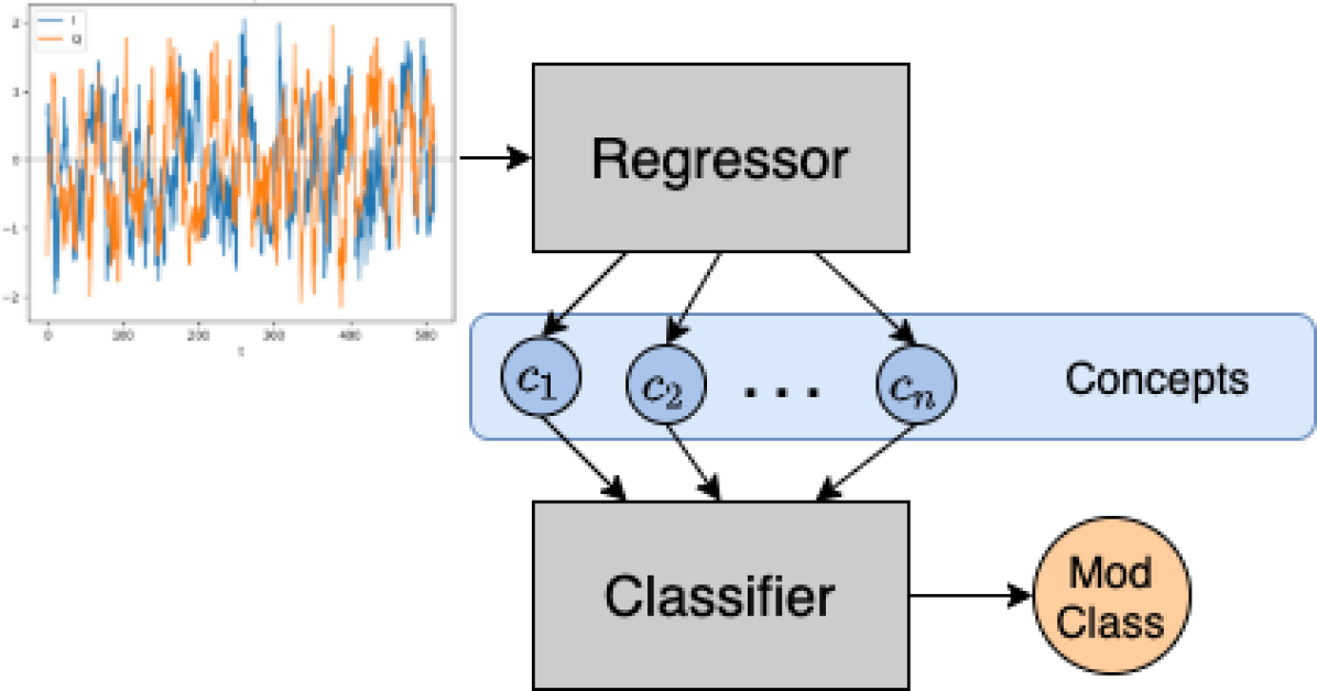
CB models first predict a set of concepts, defined during training, which are then used to make the final prediction. As a result, CB models provide inherent explainability via the predicted concepts, may enable zero-shot learning, as investigated in Section V-C, and may provide additional metrics for NN architecture selection and design. The proposed CB model-based approach, shown in Figure 1, provides the desired explainability with little-to-no loss in accuracy compared to a single-network CNN-based approach [7].

The remainder of this paper is organized as follows: First, Section II summarizes existing works related to the presented CB model-based approach. Section III describes CB models in more detail, including how the models were trained and evaluated. Then, Section IV introduces the problem space and discusses the datasets used in the work. In Section V, results are presented which examine the accuracy of the concept predictions, as well as the final classification, on a number of test sets, and investigate the feasibility of using the proposed approach for zero-shot learning. Finally, Section VI concludes the work, and discusses avenues for future work.

Figure 1: The proposed CB model-based approach to Automatic Modulation Classification.

II Related Work

II-1 Explainable RFML

Prior work in explainable RFML algorithms primarily utilize “decision tree” or “hierarchical” neural networks [8, 9, 10], which break the problem space into sub-problems, each solved using separate neural networks. For example, in [8], to solve an AMC problem, a first network determines the subgroup or modulation type of the input signal (PSK, QAM, FSK, etc.), while networks for each subgroup identify the modulation order, based on the output of the first network. In practice, networks such as these perform as well as recent single-network CNN approaches and provide some explainability, but it should be noted that in the case that the output of the first network is incorrect, the final classification will also necessarily be incorrect. Further, such decision-tree approaches tend to be more computationally and memory intensive than the single-network approach, and do not allow for zero-shot learning.

Other works utilize NN as naive feature learners and extractors in tandem with clustering techniques such as DBSCAN to increase explainability, an approach called “supervised bootstrapping,” for applications such as AMC and SEI [11, 12]. However, while supervised bootstrapping does allow for zero-shot learning, it requires hand-tuning of the clustering parameters and only provides limited explainability in the form of clustering visualizations.

II-2 Multi-task Learning

As discussed further in Section III, CB models are composed of a multi-head regression model, which performs the concept predictions, and a classifier, which utilizes the concept predictions as input to make the final classification. As a result, the proposed CB model-based approach can be viewed as a multi-task learning problem, an approach often utilized in the context of transfer learning. Other prior works in the realm of RFML have also utilized multi-task learning techniques, including the aforementioned “hierarchichal” neural networks [8], as well as for performing non-orthogonal multiple access [13].

III Concept Bottleneck Models

CB models first predict a number of concepts, provided during training, then use these predicted concepts to predict the target label. The CB model itself is composed of two networks: a multi-head regression network, $\hat{c}=g(x)$, which estimates the pre-defined concepts, $c$, using $x$ as input, and classification network, $\hat{y}=f(\hat{c})$, which predicts the target label, $y$, using only the estimated concepts, $\hat{c}$, as input. As a result, the regressor acts as a “bottleneck” in data flow. For the given AMC problem, $x$ is the raw IQ data in the form of a $2\times 128$ vector, and $y$ is the modulation scheme.

III-1 Learning Concept Bottleneck Models

As in the original CB work [6], three training regimes are examined in the results below: Independent, Sequential, and Joint. A standard trained network is included as a baseline.

1. The independent bottleneck learns $\hat{y}=\hat{f}(c)$ and $\hat{c}=\hat{g}(x)$ separately. During testing, $\hat{y}=\hat{f}(\hat{g}(x))$.

2. The sequential bottleneck learns $\hat{c}=\hat{g}(x)$ first, then learning $\hat{y}=\hat{f}(\hat{c})$.

3. The joint bottleneck trains both networks at once, learning $\hat{y}=\hat{f}(\hat{g}(x))$.

4. The standard model does not learn concepts, and rather learns $\hat{y}=\hat{f}(x)$.

Of the CB regimes, the independent bottleneck method is most efficient as the regressor and classifier can be trained in parallel. However, any error in the regressor is not considered in training the classifier, as the classifier is trained using the pristine concepts, $c$, as input, rather than those predicted by the regressor, $\hat{c}$. The sequential bottleneck method rectifies this shortcoming by training the classifier with concepts predicted by the regressor, $\hat{c}$, however, the two networks are trained with two independent loss functions. The joint bottleneck is the most complex method, as it utilizes a single loss function for training both networks. Specifically, this approach utilizes a weighted loss term, and therefore introduces an additional hyper-parameter which specifies the weight of the classifier’s loss term in relation to the regressor’s loss terms.

III-2 Concept Selection

The choice of concepts making up $c$ is largely a design choice, and is task specific. However, it should be noted that the chosen concepts must completely describe the label space, as no auxiliary data can flow through the network in it’s current form [14]. In this work, $c$ is a vector containing the following five values, selected to provide maximal explainability:

• $c_{M}=I_{M}(x):=\begin{cases}$1$&\text{if $x$ is Analog,}\\ $0$&\text{if $x$ is Digital.}\end{cases}$

• $c_{A}=I_{A}(x):=\begin{cases}$1$&\text{if $x$ is Amplitude Modulated,}\\ $0$&\text{Otherwise.}\end{cases}$

• $c_{P}=I_{P}(x):=\begin{cases}$1$&\text{if $x$ is Phase Modulated,}\\ $0$&\text{Otherwise.}\end{cases}$

• $c_{F}=I_{F}(x):=\begin{cases}$1$&\text{if $x$ is Frequency Modulated,}\\ $0$&\text{Otherwise.}\end{cases}$

• $c_{O}=\begin{cases}\frac{1}{\log_{2}(order(x))}&\text{if $order(x)$ is Defined,}\\ $\qquad 0$&\text{if $order(x)$ is Undefined. }\end{cases}$

TABLE I: Regressor architecture.

Layer Type	Num Kernels/Nodes	Kernel Size	Padding
Input	size = (2, 128)
Conv2d	96	(1, 21)	(0, 10)
ReLU
Dropout	rate = 0.5
Conv2d	96	(2, 21)	(0, 10)
ReLU
Dropout	rate = 0.5
Flatten
Linear	384
ReLU
Dropout	rate = 0.5
Linear	5
Trainable Parameters: 9830313

TABLE II: Classifier architecture.

Layer Type	Num Nodes
Input	5
Linear	64
ReLU
Dropout	rate = 0.5
Linear	64
ReLU
Dropout	rate = 0.5
Dense	9
Trainable Parameters: 5129

III-3 Model Description

In this work, the concept regressor is a CNN with five regression heads, each using a MSE loss function, equally weighted during training. The classifier is an MLP and uses a Categorical Cross Entropy loss function. These architectures were chosen using a number of hyper-parameter sweeps. The baseline CNN simply is a slightly wider version of that used in [7], and is identical to the regression architecture, with a softmax output layer instead the 5 regression heads. The specifications for each of these networks is given in Tables I and II.

Additionally, for the models trained using the joint bottleneck training regime, the classifier’s loss makes up 0.3 of the total loss, with the remaining 0.7 equally distributed amongst the regression heads. As a result, the classifier’s loss is weighed approximated double that of any single regression head in the total loss term. This hyper-parameter was chosen using additional hyper-parameter sweeps.

All models used in this work were trained using the Adam optimizer with a learning rate of 0.0001. Each regressor was trained for 200 epochs and each classifier was trained for 100 epochs, both with checkpoints saved at epochs with the lowest validation loss.

IV Problem Space and Dataset

TABLE III: In-Set Signals and Generation Parameters

Modulation Name	Symbol Order	Parameter Space
BPSK	2	RRC Pulse Shape Excess Bandwidth {0.35, 0.5} Symbol Overlap {3, 5}
QPSK	4	RRC Pulse Shape Excess Bandwidth {0.35, 0.5} Symbol Overlap {3, 5}
8PSK	8	RRC Pulse Shape Excess Bandwidth {0.35, 0.5} Symbol Overlap {3, 5}
16QAM	16	RRC Pulse Shape Excess Bandwidth {0.35, 0.5} Symbol Overlap {3, 5}
64QAM	64	RRC Pulse Shape Excess Bandwidth {0.35, 0.5} Symbol Overlap {3, 5}
FSK	2	Rect Phase Shape Carrier Spacing 5kHz, 75kHz
AM	-	DSB Mode Modulation Index [0.5, 0.9]
FM-NB	-	Modulation Index [0.05, 0.4]
AWGN	-

TABLE IV: Out-of-Set Signals and Generation Parameters

Modulation Name	Symbol Order	Parameter Space
16PSK	16	RRC Pulse Shape Excess Bandwidth {0.35, 0.5} Symbol Overlap {3, 5}
32QAM	32	RRC Pulse Shape Excess Bandwidth {0.35, 0.5} Symbol Overlap {3, 5}
MSK	2	Rect Phase Shape Carrier Spacing 2.5kHz
GFSK	2	Gaussian Phase Shape Carrier Spacing 5kHz, 75kHz Symbol Overlap {2, 4} Beta {0.3, 0.5}
AM	-	LSB Mode Modulation Index [0.5, 0.9]
FM-WB	-	Modulation Index [0.825, 1.88]

For this work, all signals which compose the training, validation, and test sets are observed at complex baseband, as given by

$$s[t]=\alpha_{\Delta}[t]\cdot\alpha[t]e^{j\omega[t]+j\theta[t]}\cdot e^{(j\omega_{\Delta}[t]+j\theta_{\Delta}[t])}+\nu[t]$$

where $\alpha[t]$ represents instantaneous magnitude, $\omega[t]$ represents instantaneous frequency, and $\theta[t]$ represents instantaneous phase, at time $t$. Frequency offsets are selected uniformly at random on the interval $[-0.1\pi,0.1\pi]$ and are held constant for each signal realization (i.e. $\omega_{\Delta}[t]=U(-0.1\pi,0.1\pi))$, and no phase offset is applied (i.e. $\theta_{\Delta}[t]=0$). All signals are sampled at either 4 or 8 samples per symbol, or 2 or 4 times Nyquist.

Additionally, all signals are observed in an AWGN environment with unit channel gain (i.e. $\alpha_{\Delta}[t]=1$), where $\nu[t]$ describes the additive interference or noise at time $t$. For each capture, the value of $\nu[t]$ is defined such that the SNR, defined as

$$\Gamma_{s}=10\log_{10}\bigg{(}\frac{\sum_{t=0}^{N-1}\lvert s[t]-\nu[t]\rvert^{2}}{\sum_{t=0}^{N-1}\lvert\nu[t]\rvert^{2}}\bigg{)}$$

is an integer value selected uniformly at random on the interval $[0,20]$dB for a capture containing $N$ samples.

The problem space is further constrained to the 15 modulation schemes shown in Tables III and IV. From these modulation schemes, three categories of signals are defined:

• in-set: includes modulation schemes given in Table III, observed during training, validation, and testing.

• near-set: includes modulation schemes in Table III, observed during testing with SNR selected uniformly at random on the intervals $[-5,-1]$dB and $[21,25]$dB. Used to measure the models ability to generalize.

• out-of-set: includes modulation schemes show in Table IV, which are only seen during testing, with the parameters as given, to gauge the zero-shot learning capabilities of the CB approach.

This work utilizes training, validation, and testing composed of synthetic signals generated using a custom Python wrapper around liquid-dsp [15]. The training set contained 10000 examples per class (90000 total), and the validation set contained 5000 examples per class (45000 total). Additionally, three test sets were used to evaluate the performance of the approach on in-set signals, near-set signals, and out-of-set signals, each of which contained 10000 examples per class (90000, 80000, and 60000 total).

V Results

As previously described in Section III, one regressor and classifier architecture is evaluated across the three CB training methods (Independent, Sequential, and Joint) and the three test datasets (In-Set, Near-Set, and Out-of-Set). In the following subsections, the performance of these models is compared to each other to identify the strengths and weaknesses of each training method, as well as to a baseline CNN architecture.

V-A Classifier Performance

Figure 2: In-set accuracy versus SNR for all three concept bottleneck models and the baseline CNN model.

(a) Independent

(b) Sequential

(c) Joint

(d) Baseline CNN

Figure 3: Confusion matrices for each learning scheme on the in-set test data.

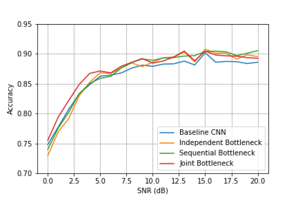
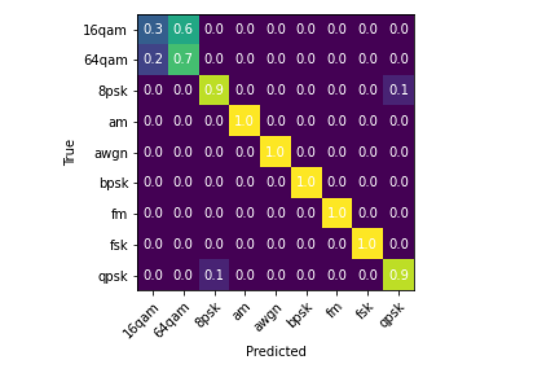
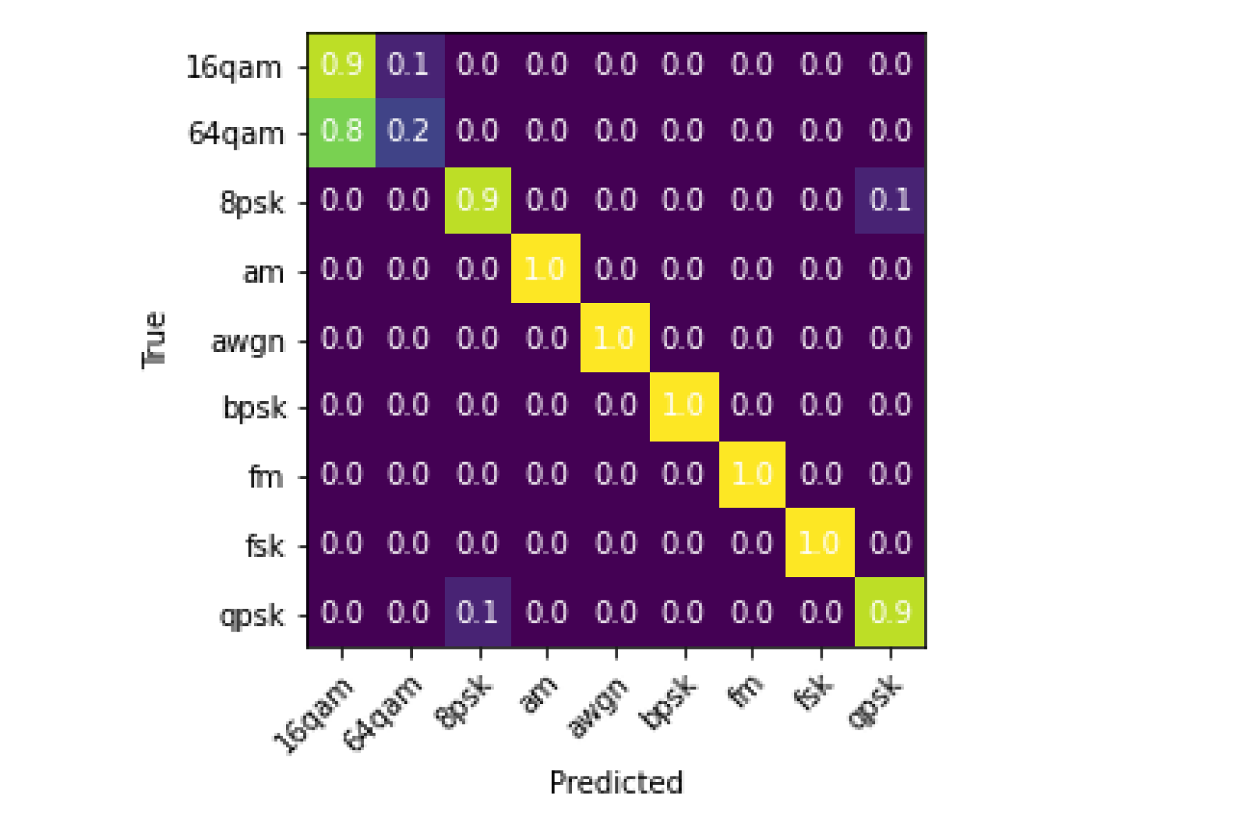
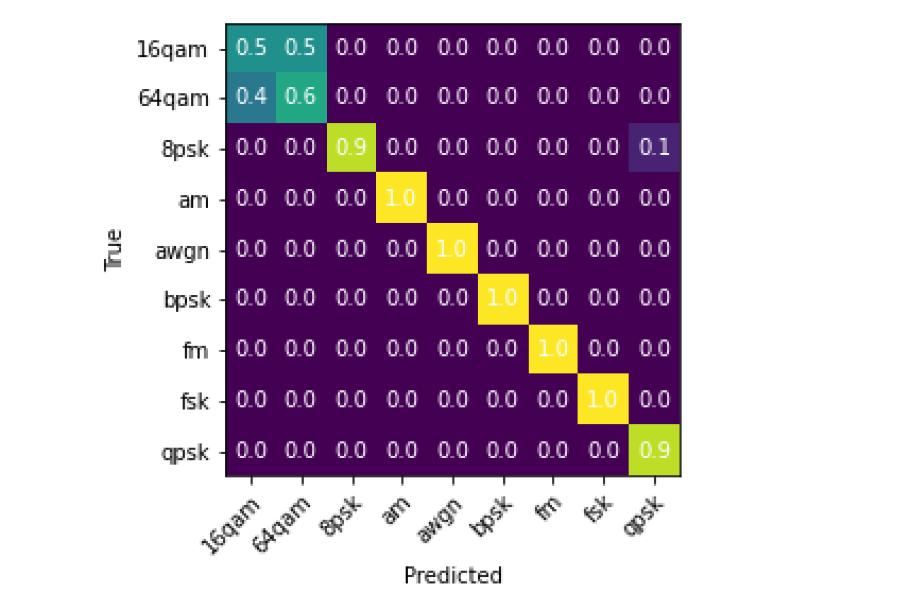
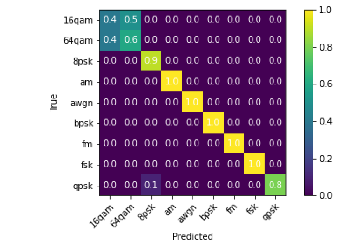
Considering first the in-set classification accuracy of each CB model in comparison to the baseline CNN approach in Table V and Figure 2. Both of these figures indicate that the CB models marginally outperform the baseline CNN approach on the in-set test dataset. Furthermore, all three CB models achieve overall in-set accuracies within 1% of each other, with the Joint model achieving the highest in-set classification accuracy of 87.24%. Additionally, Figure 3 shows that the primary source of confusion for all models, including both the CB models and baseline CNN, is 16QAM and 64QAM, which is to be expected, particularly at low SNR.

TABLE V: In-set and near-set classification accuracy for all models, averaged over all SNR.

Model	In-Set Accuracy	Near-Set Accuracy
Baseline CNN	0.8622	0.6836
Independent Bottleneck	0.8667	0.7151
Sequential Bottleneck	0.8693	0.7037
Joint Bottleneck	0.8724	0.6880

Table V also shows that all three CB models outperform the baseline CNN approach on the near-set test dataset. However, while the Joint model outperformed the Independent and Sequential models on the in-set test data, the opposite is true in the case of the near-set test data. That is, the Independent model, which was the lowest performing amongst the CB models on the in-set data, is the highest performing on the near-set test data.

V-B Regressor Performance

(a) Binary regression heads.

(b) Order regression head.

Figure 4: Performance of regression heads on in-set data.

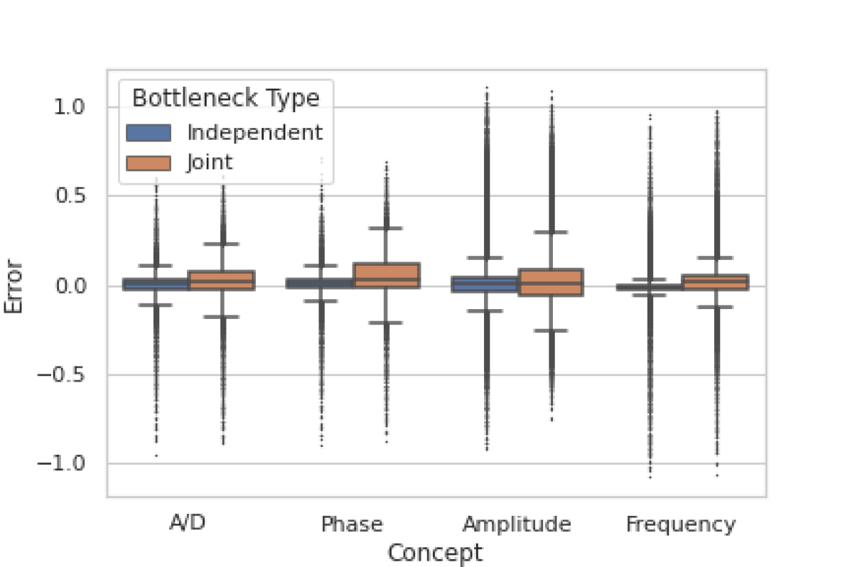
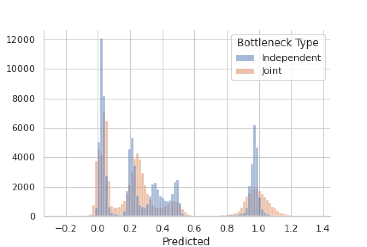
One of the primary benefits of the proposed CB model-based approach over the baseline CNN-based approach is the availability of decision explanations in the form of the intermediate predicted concepts. The accuracy of these predicted concepts on the in-set test dataset is shown in Figure 4. More specifically, for the Independent Bottleneck and Joint Bottleneck models, Figure 4(a) plots the error in the regression heads with binary truth values (A/D, Phase, Amplitude, and Frequency) in the form of a box-plot and Figure 4(b) plots the predicted order (more specifically the concept, $\hat{c}_{O}$) in the form of a histogram. Note that the Independent and Sequential models differ only in the classifier models, and utilize the same regressor models. Therefore, results in this section are shown for the Independent and Joint Bottleneck regressors only.

Figure 4(a) shows that both the Independent and Joint models predict the binary concepts with low error on in-set data. However, the Independent model shows stronger overall regression performance than the Joint Bottleneck model, despite the fact that the Joint Bottleneck outperforms the Independent and Sequential Bottleneck models in terms of overall accuracy. This result is evident in Figure 4(b) as well, where the histogram of the Independent Bottleneck model order regression-head contains all five peaks, while the histogram of the Joint Bottleneck model order regression-head only contains four peaks and has created a single output range for the higher order modulation schemes: 16 and 64.

These trends show that the Joint training regime results in marginally improved overall accuracy at the cost of losing some model explainability, as the accuracy of the concept predictions decreases. In addition to providing more transparent models, the Independent and Sequential training regimes also result in models more robust to near-set input. Therefore, the choice of training regime is dependent upon the relative importance of explainablity and classification accuracy to the designer/end-user. More specifically, the Independent model is the most explainable and robust to near-set input, the Joint model provides the highest in-set classification accuracy, and the Sequential model provides a sort of middle ground with quality decision explanations and good in-set and near-set classification accuracy.

V-C Zero-shot Learning

Another significant benefit of using the CB model-based approach over the baseline CNN-based approach is the potential for zero-shot learning, or the ability to classify signals outside of the training distribution, whether that be near-set or out-of-set (as described in Section IV). While the classification accuracy of the proposed CB approach on the near-set test dataset was discussed previously, this section examines the performance of the CB regression models on both the near-set and out-of-set test datasets. More accurate regression models, especially on the near-set and out-of-set test datasets, points to better zero-shot learning performance. To implement zero-shot learning in the proposed CB framework, the classifier component of the CB model would need to be re-trained, augmenting the training dataset with examples, ($c_{R}$, $y_{R}$), where $c_{R}$ are the concepts and $y_{R}$ are the target labels for the new signals of interest. However, this is left for future work.

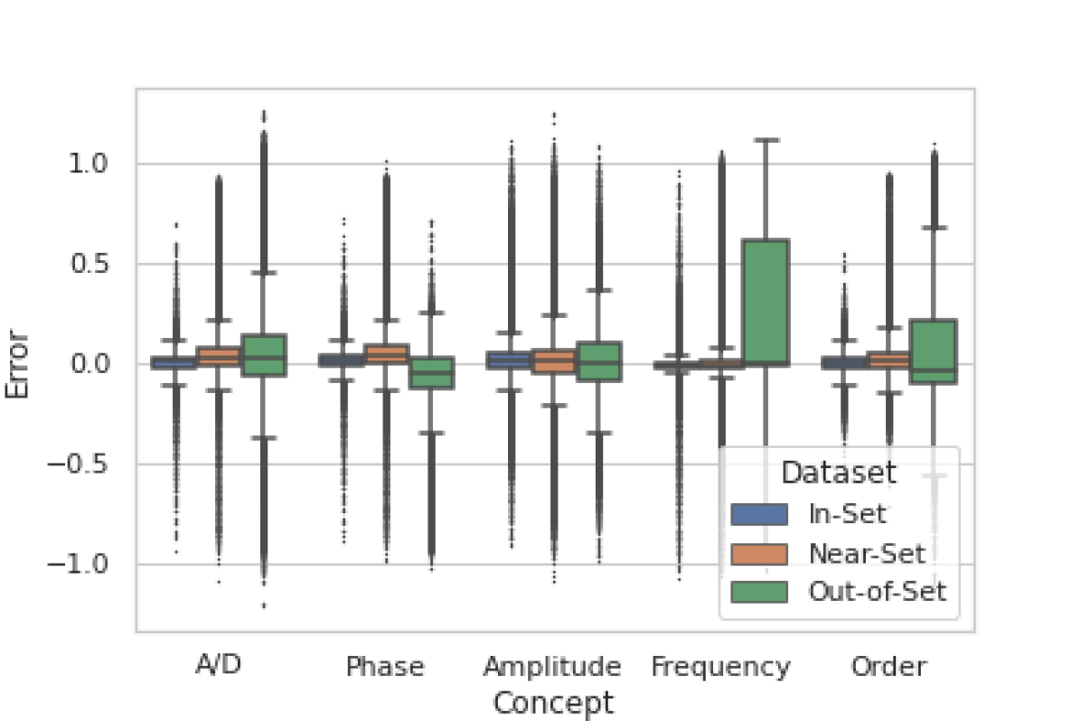
Figure 5 compares the prediction error across the three test datasets, and shows similar regression performance between the in-set and near-set datasets, which echos the classification results shown in Table V. However, while the A/D, Phase, and Amplitude binary regression heads continue to perform well on the out-of-set test dataset, Frequency and order prediction performance declines.

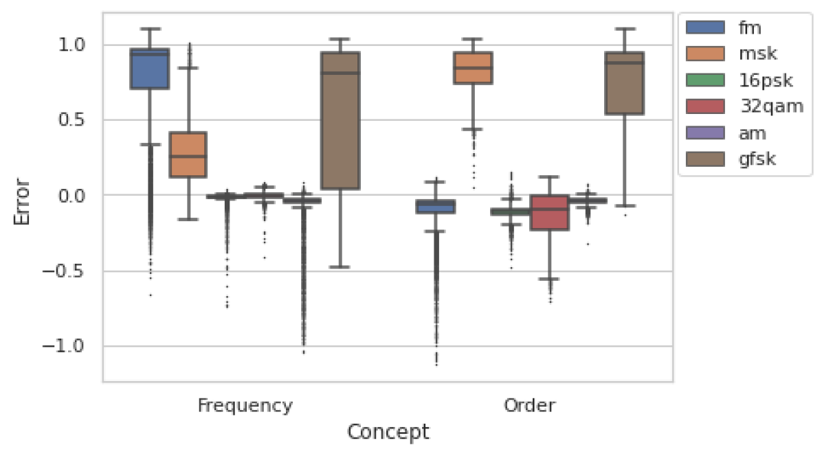
Figure 6 expands upon the results given in figure 5 by breaking out the performance of the Frequency and order regression heads by modulation scheme on the out-of-set signal types, and shows that for these more challenging concepts, FM-WB, GFSK, and MSK are most challenging for the regression model to accurately assess. Intuitively, these modulation schemes differ most from the in-set modulation schemes, in comparison to the remaining out-of-set modulation schemes, namely 16PSK, 32QAM, and AM-LSB. This result echos those shown in the zero-shot learning literature which indicate that algorithms similar to the CB approach often suffer when the source data and target data are disjoint [16]. Therefore, CB model-based zero-shot learning is likely feasible for near-set signal types and signal types which are similar to those seen in training. However, further work is likely needed to improve the accuracy of the regression model to improve zero-shot learning performance on out-of-set signal types.

VI Conclusion

Figure 5: Regression performance across the in-set, near-set, and out-of-set data types for the Independent Bottleneck model.

In this work, CB models were investigated as a means to provide decision explanations in the context of a DL-based AMC algorithm. The approach provides inherent decision explanations, in the form of intermediate concept predictions, in addition to the predicted modulation class, using only raw IQ data as input.

The approach was evaluated across three training regimes and three test sets containing in-set, near-set, and out-of-set data. Results show the CB models achieve similar classification accuracy to a recent single-network AMC algorithm on in-set data, and outperforms said algorithm on the near-set test dataset. Further, the proposed approach shows promise evaluating signal types unseen in training (out-of-set data) using the intermediate predicted concepts, a setting known as zero-shot learning.

Most apparently, future work includes applying the CB to other RFML applications, and improving accuracy through the use of more sophisticated architecures, loss functions, and hyper-parameter tuning. In particular, the regression component of the CB model needs improvement if zero-shot learning is desired, another avenue for future work. The accuracy of the intermediate concept predictions could also be investigated as another set of metrics for NN architecture selection. Finally, a more intriguing avenue for future work includes debiasing the model using a causal prior graph, to eliminate correlations between the intermediate concepts and spurious features such as SNR [14].

Figure 6: Out-of-set frequency and order prediction using the Independent Bottleneck model broken out by modulation scheme.

References

- [1] T. Rondeau, “Radio frequency machine learning systems (RFMLS).” [Online]. Available: https://www.darpa.mil/program/radio-frequency-machine-learning-systems
- [2] L. J. Wong, W. H. Clark, B. Flowers, R. M. Buehrer, A. J. Michaels, and W. C. Headley, “The rfml ecosystem: A look at the unique challenges of applying deep learning to radio frequency applications,” 2020.
- [3] M. E. Morocho-Cayamcela, H. Lee, and W. Lim, “Machine learning for 5G/B5G mobile and wireless communications: Potential, limitations, and future directions,” IEEE Access, vol. 7, pp. 137 184–137 206, 2019.
- [4] D. V. Carvalho, E. M. Pereira, and J. S. Cardoso, “Machine learning interpretability: A survey on methods and metrics,” Electronics, vol. 8, no. 8, p. 832, 2019.
- [5] O. A. Dobre, A. Abdi, Y. Bar-Ness, and W. Su, “Survey of automatic modulation classification techniques: classical approaches and new trends,” IET Communications, vol. 1, no. 2, pp. 137–156, 2007.
- [6] P. W. Koh, T. Nguyen, Y. S. Tang, S. Mussmann, E. Pierson, B. Kim, and P. Liang, “Concept bottleneck models,” arXiv preprint arXiv:2007.04612, 2020.
- [7] T. J. O’Shea, J. Corgan, and T. C. Clancy, “Convolutional radio modulation recognition networks,” in Engineering Applications of Neural Networks, C. Jayne and L. Iliadis, Eds. Cham: Springer International Publishing, 2016, pp. 213–226.
- [8] W. H. Clark, V. Arndorfer, B. Tamir, D. Kim, C. Vives, H. Morris, L. J. Wong, and W. C. Headley, “Developing RFML intuition: an automatic modulation classification architecture case study,” in MILCOM 2019 - 2019 IEEE Military Communications Conference (MILCOM), Oct 2019.
- [9] K. Karra, S. Kuzdeba, and J. Petersen, “Modulation recognition using hierarchical deep neural networks,” in 2017 IEEE International Symposium on Dynamic Spectrum Access Networks (DySPAN), 2017, pp. 1–3.
- [10] G. Vanhoy, N. Thurston, A. Burger, J. Breckenridge, and T. Bose, “Hierarchical modulation classification using deep learning,” in MILCOM 2018 - 2018 IEEE Military Communications Conference (MILCOM), 2018, pp. 20–25.
- [11] T. J. O’Shea, N. West, M. Vondal, and T. C. Clancy, “Semi-supervised radio signal identification,” in 2017 19th International Conference on Advanced Communication Technology (ICACT), 2017, pp. 33–38.
- [12] L. J. Wong, W. C. Headley, S. Andrews, R. M. Gerdes, and A. J. Michaels, “Clustering learned cnn features from raw i/q data for emitter identification,” in MILCOM 2018 - 2018 IEEE Military Communications Conference (MILCOM), 2018, pp. 26–33.
- [13] G. Gui, H. Huang, Y. Song, and H. Sari, “Deep learning for an effective nonorthogonal multiple access scheme,” IEEE Transactions on Vehicular Technology, vol. 67, no. 9, pp. 8440–8450, 2018.
- [14] M. T. Bahadori and D. E. Heckerman, “Debiasing concept bottleneck models with instrumental variables,” arXiv preprint arXiv:2007.11500, 2020.
- [15] J. Gaeddert, “liquid-dsp.” [Online]. Available: https://github.com/jgaeddert/liquid-dsp
- [16] Y. Fu, T. M. Hospedales, T. Xiang, and S. Gong, “Transductive multi-view zero-shot learning,” IEEE transactions on pattern analysis and machine intelligence, vol. 37, no. 11, pp. 2332–2345, 2015.