The Evolution of the Lyman-Alpha Luminosity Function During Reionization

Abstract

The time frame in which hydrogen reionization occurred is highly uncertain, but can be constrained by observations of Lyman-alpha (Ly$\alpha$) emission from distant sources. Neutral hydrogen in the intergalactic medium (IGM) attenuates Ly$\alpha$ photons emitted by galaxies. As reionization progressed the IGM opacity decreased, increasing Ly$\alpha$ visibility. The galaxy Ly$\alpha$ luminosity function (LF) is thus a useful tool to constrain the timeline of reionization. In this work, we model the Ly$\alpha$ LF as a function of redshift, $z=5-10$, and average IGM neutral hydrogen fraction, $\overline{x}_{\textsc{hi}}$. We combine the Ly$\alpha$ luminosity probability distribution obtained from inhomogeneous reionization simulations with a model for the UV LF to model the Ly$\alpha$ LF. As the neutral fraction increases, the average number density of Ly$\alpha$ emitting galaxies decreases, and are less luminous, though for $\overline{x}_{\textsc{hi}}\lesssim 0.4$ there is only a small decrease of the Ly$\alpha$ LF. We use our model to infer the IGM neutral fraction at $z=6.6,7.0,7.3$ from observed Ly$\alpha$ LFs. We conclude that there is a significant increase in the neutral fraction with increasing redshift: $\overline{x}_{\textsc{hi}}(z=6.6)=0.08^{+0.08}_{-0.05},\,\overline{x}_{\textsc{hi}}(z=7.0)=0.28\pm 0.05$ and $\overline{x}_{\textsc{hi}}(z=7.3)=0.83^{+0.06}_{-0.07}$. We predict trends in the Ly$\alpha$ luminosity density and Schechter parameters as a function of redshift and the neutral fraction. We find that the Ly$\alpha$ luminosity density decreases as the universe becomes more neutral. Furthermore, as the neutral fraction increases, the faint-end slope of the Ly$\alpha$ LF steepens, and the characteristic Ly$\alpha$ luminosity shifts to lower values, concluding that the evolving shape of the Ly$\alpha$ LF – not just its integral – is an important tool to study reionization.

1 Introduction

After Recombination, $\sim 75\%$ of the baryons in the early universe were atomic hydrogen. In the present-day universe, the majority of hydrogen in the intergalactic medium (IGM) is ionized. At some point within the first billion years, ionizing photons, likely emitted by the first stars and galaxies, reionized hydrogen during this ‘Epoch of Reionization’, initially in bubbles around galaxies which eventually overlapped and created an entirely ionized IGM (e.g., Barkana & Loeb, 2007; Mesinger, 2016; Dayal & Ferrara, 2018).

The time frame in which reionization occurred is still highly uncertain. Its onset and progression are rather poorly constrained (e.g., Greig et al., 2017; Mason et al., 2019a). The best constraints currently come from observations of the increasing optical depth to Ly$\alpha$  photons, observed in the spectra of high redshift quasars (e.g., Fan et al., 2006; McGreer et al., 2015; Bañados et al., 2018; Davies et al., 2018; Greig et al., 2017) and galaxies – both those selected as Lyman-break galaxies (e.g., Treu et al., 2013; Schenker et al., 2014; Mesinger et al., 2014; Mason et al., 2018, 2019b; Hoag et al., 2019; Whitler et al., 2020; Jung et al., 2020) and Lyman-alpha emitters (e.g., Malhotra & Rhoads, 2004; Konno et al., 2018). These constraints imply a fairly late and rapid reionization (e.g., Mason et al., 2019a; Naidu et al., 2020), though c.f. Finkelstein et al. (2019); Jung et al. (2020) who find evidence for a slightly earlier reionization. During reionization, Ly$\alpha$ photons are attenuated extremely effectively by neutral hydrogen (e.g., Miralda-Escudé, 1998; Mesinger et al., 2014; Mason et al., 2018). As a result, Ly$\alpha$ observations can be an investigative tool of the neutral IGM during the Epoch of Reionization. However, these reionization inferences are limited by systematic uncertainties in modelling the intrinsic Ly$\alpha$ emission – more independent probes are necessary to understand the systematic uncertainties in reionization inferences.

In this paper, we use the Lyman-alpha (Ly$\alpha$ ) luminosity function to constrain the progression of reionization with cosmic time. Ly$\alpha$ luminosity functions (LFs) have been used for over a decade to understand reionization (e.g., Rhoads & Malhotra, 2001; Malhotra & Rhoads, 2004; Stern et al., 2005; Jensen et al., 2013). LFs describe the luminosity distribution of a population of objects and we can quantify their evolution by looking at the LF at different redshifts. As Ly$\alpha$ is typically expected to be the strongest emission line in the rest-frame optical to UV (e.g., Partridge & Peebles, 1967; Shapley et al., 2003), wide-area ground-based narrow-band surveys (e.g., Malhotra & Rhoads, 2004; Ota et al., 2008, 2010; Ouchi et al., 2010; Konno et al., 2014; Konno et al., 2016; Ota et al., 2017; Konno et al., 2018) and, more recently, space-based grism observations (e.g., Tilvi et al., 2016; Bagley et al., 2017; Larson et al., 2018) have been efficient at discovering large populations of galaxies at high redshifts, selected based on strong Ly$\alpha$ fluxes, and known as ‘Ly$\alpha$ emitters’ or LAEs.

As Ly$\alpha$ photons are obscured during reionization, a decline in the Ly$\alpha$ LF is a signature of an increasingly neutral IGM. However, any evolution must be disentangled from the evolution in the underlying galaxy population with redshift (i.e., as galaxies become less numerous at high redshifts due to hierarchical structure formation). Previous works typically compared the evolution of the Ly$\alpha$ LF to that of the UV LF, which describes the number density of Lyman-break galaxies and is not distorted by reionization, to establish the evolution due to neutral gas (e.g., Ouchi et al., 2008, 2010; Konno et al., 2018; Konno et al., 2016). These works estimated the neutral fraction at specific redshifts by using the drop in the Ly$\alpha$ luminosity density compared to the UV luminosity density to calculate a transmission fraction, $T_{\mathrm{IGM}}$, the fraction of Ly$\alpha$ flux transmitted through the IGM, under the assumption $T_{\mathrm{IGM}}$ does not depend on Ly$\alpha$ or UV luminosity.

However, due to the inhomogeneous nature of reionization (e.g., Miralda-Escudé et al., 2000; Ciardi et al., 2003; Furlanetto & Oh, 2005; Mesinger, 2016), the transmission fraction is in reality a broad distribution, which is not captured by the luminosity density estimates. Importantly, Mason et al. (2018) demonstrated the transmission fraction depends on not only the the average neutral fraction of hydrogen in the IGM, but also the galaxy’s local environment and emission properties. For example, UV-bright galaxies have a higher transmission fractions at all neutral fraction values because their Ly$\alpha$ line profiles are typically redshifted far into the damping wing absorption profile and they also typically exist in large reionized bubbles early in reionization (Mason et al., 2018; Whitler et al., 2020). By contrast, UV-faint galaxies emit Ly$\alpha$ closer to their systemic velocity, which is thus more significantly absorbed by surrounding neutral IGM. They can be found in under-dense regions of the cosmic web where the IGM is still neutral, resulting in a lower transmission fraction even for high average neutral fractions.

This work models the evolution of the Ly$\alpha$ LF as a function of the volume average neutral hydrogen fraction, $x_{\textsc{hi}}$ , and redshift, z, to interpret observations and constrain reionization. We create our model by convolving the UV LF with the Ly$\alpha$ luminosity probability distribution as a function of $M_{\textsc{uv}}$ . The models in this project include realistic, inhomogeneous simulations for reionization, enabling us to include the full distribution of Ly$\alpha$ transmissions. This is an improvement on previous work which interpreted the Ly$\alpha$ LF using fixed Ly$\alpha$  transmission fractions (e.g., Konno et al., 2018; Hu et al., 2019), which may be considered an oversimplification. Furthermore, we use an analytic approach that enables us to model the Ly$\alpha$ LF as a function of $x_{\textsc{hi}}$ and $z$ independently, rather than using a simulation with a fixed reionization history (e.g., Itoh et al., 2018) – allowing us to disentangle the impact of IGM and redshift evolution.

This paper is structured as follows. In Section 2 we describe our model for the Ly$\alpha$ LF. In Section 3 we describe our results for the Ly$\alpha$ LF and the evolution of the Schechter function parameters and luminosity density. We infer the evolution of the neutral fraction for $z>6$ by fitting our model to observations and we forecast predictions for future surveys with the Nancy Grace Roman Space Telescope, Euclid, and the James Webb Space Telescope. In Section 4 we discuss our results and we present our conclusions in Section 5.

We use the Planck Collaboration et al. (2016) cosmology and all magnitudes are given in the AB system.

2 Methods

Here, we describe the components of our model. In Section 2.1, we describe the methodology used to model the Ly$\alpha$ LF. Both model components – the Ly$\alpha$ luminosity probability distribution and the UV LF – are described in the succeeding Sections 2.1.1 and 2.2. Section 2.3 describes the normalization of the Ly$\alpha$ LF. Section 2.4 describes the Bayesian framework used to infer the neutral fraction given the Ly$\alpha$ LF model and observational data. In Section 2.5 we discuss the differences in observational datasets that led to omitting or including certain surveys in our analysis.

2.1 Modelling the Ly$\alpha$ luminosity function

We model the evolution of the Ly$\alpha$ LF as a function of redshift and $x_{\textsc{hi}}$ by convolving models for the Ly$\alpha$ emission from Lyman-break galaxies (LBGs) and the UV LF during reionization. This enables us to disentangle the effects of redshift evolution from the evolution due to IGM absorption (Mason et al., 2015b; Mesinger, 2016; Mason et al., 2018).

The luminosity function (LF) of galaxies shows the number density of galaxies in a certain luminosity interval and is typically described using the Schechter (1976) function:

$$\phi(L)\mathrm{d}L=\phi^{*}\left(\frac{L}{L^{*}}\right)^{\alpha}\exp{\left(-\frac{L}{L^{*}}\right)}\,\mathrm{d}\left(\frac{L}{L^{*}}\right)$$ (1)

where $\phi^{*}$ is the normalization constant, $\alpha$ is the power law for faint-end slope for $L<L^{*}$, and there is an exponential cutoff at $L>L^{*}$. These parameters are known to be conditional on the observed wavelength and cosmic time, as well as the type of galaxy (e.g., Dahlen et al., 2005). The rest-frame UV LF has been measured in detail out to $z\sim 10$ and is one of our best tools for studying the evolution of galaxy populations (e.g., Bouwens et al., 2016, 2015; Finkelstein et al., 2015a; Oesch et al., 2015).

Following Dijkstra & Wyithe (2012); Gronke et al. (2015) we can predict the number density of LAEs by using the UV LF and Ly$\alpha$ luminosity probability distribution for LBGs to model the Ly$\alpha$ LF:

$$\begin{split}\phi_{\mathrm{LAE}}&(L_{\alpha},{x_{\textsc{hi}}},z)\mathrm{d}L_{\alpha}=\mathrm{d}L_{\alpha}F\\ &\times\int_{\mathrm{M}_{\mathrm{UV,min}}}^{\mathrm{M}_{\mathrm{UV,max}}}\mathrm{d}{M_{\textsc{uv}}}\,\phi({M_{\textsc{uv}}},z)P(L_{\alpha}\,|\,{M_{\textsc{uv}}},{x_{\textsc{hi}}},z)\end{split}$$ (2)

Here, $\phi({M_{\textsc{uv}}},z)\mathrm{d}{M_{\textsc{uv}}}$ is the UV LF in the range ${M_{\textsc{uv}}}\pm\mathrm{d}{M_{\textsc{uv}}}/2$ and is described in Section 2.2. $P(L_{\alpha}\,|\,{M_{\textsc{uv}}},{x_{\textsc{hi}}})$, is the conditional probability of galaxies that have a Ly$\alpha$ luminosity $L_{\alpha}$ in $L_{\alpha}\pm\mathrm{d}L_{\alpha}/{2}$, given a $M_{\textsc{uv}}$ value and neutral fraction and is described in Section 2.1.1. We integrate our Ly$\alpha$ LF over the $M_{\textsc{uv}}$ range $-24<{M_{\textsc{uv}}}<-12$ covering the observed range of the UV LF, $-23<{M_{\textsc{uv}}}<-17$.

The factor $F$ in Equation 2 is a normalization constant to fit the LF model to observations and can be thought of as the ratio of predicted LAEs versus the total number of LAEs recorded. If the Ly$\alpha$ luminosity distribution, $P(L_{\alpha}\,|\,{M_{\textsc{uv}}},{x_{\textsc{hi}}},z)$ accurately describes the luminosities of the same Lyman-break galaxies measured in the UV LF this factor should be $F=1$ (See Section 4.3 for further discussion).

2.1.1 Ly$\alpha$ luminosity probability distribution

The probability distribution for Ly$\alpha$ luminosity is derived from the Ly$\alpha$ rest-frame equivalent width (EW) probability density function $P(EW\,|\,{M_{\textsc{uv}}})$ where $P(L_{\alpha}\,|\,{M_{\textsc{uv}}},{x_{\textsc{hi}}})=P(EW\,|\,{M_{\textsc{uv}}},{x_{\textsc{hi}}})\frac{\partial EW}{\partial L_{\alpha}}$. We use the rest-frame EW probability distribution models by Mason et al. (2018) (based on observations by De Barros et al., 2017) who forward-model observed EW after transmission through 1.6 Gpc³ inhomogeneous reionization simulations (Mesinger, 2016) at fixed average neutral fraction ${x_{\textsc{hi}}}=0.01-0.95$, with a spacing of $\Delta{x_{\textsc{hi}}}\sim 0.01-0.03$. We use the following relationship between Ly$\alpha$ luminosity in $\mathrm{erg\,s}^{-1}$ and EW to obtain $\partial EW/\partial L_{\alpha}$:

$$L_{\alpha}=EW\times L_{\textsc{uv},\nu}\times\frac{c}{\lambda_{\mathrm{Ly}\alpha}^{2}}\left(\frac{\lambda_{\mathrm{Ly}\alpha}}{\lambda_{\textsc{uv}}}\right)^{\beta+2}$$ (3)

Here, $\lambda_{\alpha}\sim 1216$ Å is the wavelength of the Ly$\alpha$ resonance, the rest-frame wavelength of the UV continuum is typically measured at $\lambda_{\textsc{uv}}\sim 1500$ Å , $\beta$ is the UV continuum slope, where we assume $\beta=-2$ typical for high redshifts (e.g., Bouwens et al., 2014), and $c$ is the speed of light. $L_{\textsc{uv},\nu}$ is the UV luminosity density:

$$L_{\textsc{uv},\nu}=4\pi(10)^{2}\times 10^{-0.4({M_{\textsc{uv}}}+48.6)}\,\mathrm{erg\,s}^{-1}\,\mathrm{Hz}^{-1}.$$ (4)

We normalize $P(L_{\alpha}\,|\,{M_{\textsc{uv}}},{x_{\textsc{hi}}})$ over the luminosity range $L_{\alpha}=0-10^{44.5}$ erg s^-1 to encompass a large Ly$\alpha$ luminosity interval, and within our defined $M_{\textsc{uv}}$ range between $-24<{M_{\textsc{uv}}}<-12$ (see Section 2.1).

The Ly$\alpha$ luminosity probability distribution, $P(L_{\alpha}\,|\,{M_{\textsc{uv}}},{x_{\textsc{hi}}})$, is shown in Figure 1 for a few $x_{\textsc{hi}}$ and $M_{\textsc{uv}}$ values. We note that as the Mason et al. (2018) models assume no evolution of the intrinsic Ly$\alpha$ EW distribution with redshift – the only redshift evolution is due to the increasing neutral fraction, our Ly$\alpha$ luminosity distribution models also depend only on ${x_{\textsc{hi}}}$ with no additional redshift evolution. Recent works by Hashimoto et al. (2017); Jung et al. (2018); Shibuya et al. (2018) confirm a suitable approach to the Ly$\alpha$ EW distribution models we incorporate into our work. Each paper ultimately notes no significant evolution in the Ly$\alpha$ EW distribution with respect to redshift for $z\sim 5-7$.

Figure 1 demonstrates large differences in the probability distribution for UV-bright and UV-faint galaxies. For UV-faint galaxies, we expect a higher probability of Ly$\alpha$ luminosity emission at all $x_{\textsc{hi}}$ values but with a Ly$\alpha$ luminosity cut off at $L_{\alpha}\,\hbox to0.0pt{\lower 3.5pt\hbox{$\mathchar 0\relax\sim$}\hss}\raise 1.0pt\hbox{$<$}\,10^{42}$ erg s^-1. For UV-bright galaxies, at all $x_{\textsc{hi}}$ we expect galaxies to have higher Ly$\alpha$ luminosity values up to $L_{\alpha}\,\hbox to0.0pt{\lower 3.5pt\hbox{$\mathchar 0\relax\sim$}\hss}\raise 1.0pt\hbox{$<$}\,10^{44}$ erg s^-1, but this is rarer. For both UV-bright and UV-faint galaxies, as the neutral fraction increases, the probability of galaxies emitting strong Ly$\alpha$ overall decreases.

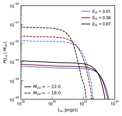
Figure 1: Example of the probability distribution for Ly$\alpha$ luminosity, $P({\mathrm{Ly}\alpha}\,|\,{M_{\textsc{uv}}},{x_{\textsc{hi}}})$. This distribution is for UV-bright (solid line) and UV-faint galaxies (dashed line) at different $x_{\textsc{hi}}$ values, ${x_{\textsc{hi}}}=0.01,0.36,0.87$. When $x_{\textsc{hi}}$ increases to an almost neutral environment, the probability of detecting luminous Ly$\alpha$ galaxies decreases compared to in an almost fully ionized environment.

The $M_{\textsc{uv}}$ dependence of $P(L_{\alpha}\,|\,{M_{\textsc{uv}}})$ is a direct consequence of the EW distribution model by Mason et al. (2018). This model can be described as an exponential distribution plus a delta function:

$$\begin{split}P(EW|{M_{\textsc{uv}}})=&\frac{A({M_{\textsc{uv}}})}{EW_{c}({M_{\textsc{uv}}})}e^{-\frac{EW}{EW_{c}({M_{\textsc{uv}}})}}H(EW)\\ &+[1-A({M_{\textsc{uv}}})]\delta(EW)\end{split}$$ (5)

where

$$A({M_{\textsc{uv}}}) =0.65+0.1\,\mathrm{tanh}[3({M_{\textsc{uv}}}+20.75)]$$ (6)

$$EW_{c}({M_{\textsc{uv}}}) =31+12\,\mathrm{tanh}[4({M_{\textsc{uv}}}+20.25)]\,\mathrm{\AA}$$ (7)

account for the fraction of emitters and the anti-correlation of EW with $M_{\textsc{uv}}$ respectively. $H(EW)$ is the Heaviside step function and $\delta(EW)$ is a Dirac delta function (see Section 2.1.3 of Mason et al., 2018 for further details). The intrinsic, emitted, distribution (i.e. ${x_{\textsc{hi}}}=0$) is an empirical model fit to observations by De Barros et al. (2017) at $z\sim 6$, where it was found that UV-bright galaxies had a lower probability of being emitters, and had lower average EWs (consistent with previous findings; e.g., Ando et al., 2006; Stark et al., 2010). The model EW distribution is then painted onto galaxies in inhomogeneous reionization simulations, with different average neutral fractions, and the ‘observed’ EW distribution in each of those simulations is recovered by sampling the transmission along thousands of sightlines.

Although bright galaxies have low EW compared to faint galaxies, they are, on average, less affected by neutral gas in the IGM: UV-bright galaxies are typically more massive and reside in dense regions of the universe, in large IGM bubbles that have already reionized. In the simulations we use, reionization occurs first in overdense regions due to the excursion set formalism (Mesinger & Furlanetto, 2007; Mesinger, 2016). Observationally, clustering analyses show that UV-bright galaxies typically live in massive halos in dense regions (e.g., Figure 15 of Harikane et al., 2018). So, Ly$\alpha$ photons can escape more easily and EWs decrease at a slower rate (transmissions are already high). UV-faint galaxies have a higher intrinsic EW, on average, that decreases more rapidly than for UV-bright galaxies as the universe becomes more neutral. This is because they can be more typically found in neutral patches of IGM.

As described above in Section 2.1, we generate our Ly$\alpha$ LF by integrating the UV LF over the $M_{\textsc{uv}}$ range $-24<{M_{\textsc{uv}}}<-12$, covering the observed range of the UV LF, $-23\lesssim{M_{\textsc{uv}}}\lesssim-17$. As the Mason et al. (2018) EW models were defined for $-23\leq{M_{\textsc{uv}}}\leq-17$ to include galaxies outside of this range we set galaxies brighter than ${M_{\textsc{uv}}}=-23$ to have the same $P(L_{\alpha}\,|\,{M_{\textsc{uv}}}=-23)$, and all galaxies fainter than ${M_{\textsc{uv}}}=-17$ have the same $P(L_{\alpha}\,|\,{M_{\textsc{uv}}}=-17)$ (for a given ${x_{\textsc{hi}}}$).

2.2 Galaxy UV luminosity functions

In this paper, we use the Mason et al. (2015b) UV LF model. In this model galaxy evolution is dependent on star formation that is associated with the construction of dark matter halos, with the assumption that these halos have a star formation efficiency that is mass dependent but redshift independent, which successfully reproduces observations over 13 Gyr (see also, e.g., Trenti et al., 2010; Tacchella et al., 2013, 2018; Mirocha et al., 2020).

The UV LF is plotted in Figure 2. It is well-described by a Schechter (1976) function (Equation 1). The steep drop off of UV-bright galaxies can be explained in terms of rare high mass halos and their star formation efficiency: high mass halos are not efficient at forming stars, likely due to strong negative active galactic nuclei (AGN) feedback. The drop in number density with increasing redshift indicates a shift in star formation towards fainter, less massive galaxies.

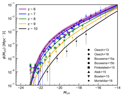
Figure 2: Modelled UV luminosity function for redshifts at $z=6-10$ for UV-bright and faint galaxies, based on Mason et al. (2015b) UV luminosity function model. There is a steep, exponential, drop-off for UV-bright galaxies that turns over into a power-law slope for UV-faint galaxies. The shaded region shows the $1\sigma$ confidence range at $z\sim 6$ and similar regions can be assumed for each redshift. UV LF observations are shown with each marker color matching its corresponding UV LF model at a given redshift. Points show the binned UV LFs and upper limits from Oesch et al. (2013, 2018); Bouwens et al. (2015, 2016); Finkelstein et al. (2015b); Atek et al. (2015); Bowler et al. (2015); Morishita et al. (2018).

2.3 Calibrating the normalization of the Ly$\alpha$ LF

To obtain an accurate model of the Ly$\alpha$ LF to compare with observations, we must calibrate the Ly$\alpha$ LF by finding the normalization constant, $F$. This factor accounts for any over-prediction in the number density of LAEs caused by the Ly$\alpha$ luminosity distribution, $P(L_{\alpha}\,|\,{M_{\textsc{uv}}},{x_{\textsc{hi}}},z)$ (Dijkstra & Wyithe, 2012; Gronke et al., 2015). If the Ly$\alpha$ luminosity distribution accurately describes the luminosities of the Lyman-break galaxies measured in the UV LF we should obtain $F=1$.

We estimate $F$ using a maximum-likelihood approach to fit our model at $z=5.7,{x_{\textsc{hi}}}\sim 0$ to the Konno et al. (2018); Ouchi et al. (2008) observations at $z=5.7$. We set calibration at this redshift and neutral fraction as it is likely to be after the end of reionization (e.g., McGreer et al., 2015). Note, due to our reionization simulation grid (see Section 2.1.1), we use ${x_{\textsc{hi}}}=0.01$ for calibration, rather than ${x_{\textsc{hi}}}=0.0$, but note that the difference in $P(L_{\alpha}|{M_{\textsc{uv}}},{x_{\textsc{hi}}})$ should be negligible for such a small change in neutral fraction (as shown by Mason et al., 2018).

We maximise the likelihood for the observed Ly$\alpha$ LFs in each luminosity bin $L_{i}$: $P(\phi_{i}\,|\,\theta=F,L_{i},\sigma_{i})$ given our model $\phi_{\mathrm{mod}}(\theta=F,L)$. This estimation using binned LFs may not be the most optimal: a more accurate likelihood would be obtained using individual source information and the survey selection function (see e.g., Trenti & Stiavelli, 2008; Kelly et al., 2008; Schmidt et al., 2014; Mason et al., 2015a), however collating of these data is not feasible within the scope of this project, and we leave this for future works. We note that Trenti & Stiavelli (2008) demonstrated that LFs estimated from binned data are generally in good agreement with those measured from unbinned data, but can bias the faint end slope towards steeper values. However, as the observed high-redshift Ly$\alpha$ LFs are mostly $\,\hbox to0.0pt{\lower 3.5pt\hbox{$\mathchar 0\relax\sim$}\hss}\raise 1.0pt\hbox{$>$}\,L^{*}$, we do not expect this to have a large impact on our results as the faint-end will already have large uncertainties.

Following Gillet et al. (2020) we use a split-norm likelihood (Equation 9), to take into account asymmetric error bars. Assuming each observation and luminosity bin are independent, the total likelihood is:

$$P(\phi_{obs}\,|\,\theta=F,L)=\prod_{i}S(\phi_{\mathrm{mod}}(F,L_{i}),\mu_{i},\sigma_{1,i},\sigma_{2,i})$$ (8)

Here, $\phi_{\mathrm{mod}}(F,L_{i})$ is the model LF at luminosity $L_{i}$ for parameter $\theta=F$, $\mu_{i}$ is the observed number density value at $L_{i}$, and $\sigma_{1,i}$ and $\sigma_{2,i}$ are the respective lower and upper errors of the observed number density. In a single luminosity bin:

$$S(\phi_{\mathrm{mod}}) =\begin{cases}B\exp[-\frac{1}{2}\frac{(\phi_{\mathrm{mod}}-\mu)^{2}}{\sigma_{1}^{2}}]&\text{if $\phi_{\mathrm{mod}}\leq\mu$}\\ B\exp[-\frac{1}{2}\frac{(\phi_{\mathrm{mod}}-\mu)^{2}}{\sigma_{2}^{2}}]&\text{if $\phi_{\mathrm{mod}}\geq\mu$}\\ \end{cases}$$ (9)

$$B =\left[\sqrt{2\pi}\left(\frac{\sigma_{1}+\sigma_{2}}{2}\right)\right]^{-1}$$ (10)

We minimize the logarithm of the likelihood Equation 8 to find $F$ using the Python package SciPy minimize. The obtained minimum value is $F=0.974$ which we then use for Ly$\alpha$ LF at all redshifts and $x_{\textsc{hi}}$ values.

Our recovered value of $F\approx 1$ indicates our luminosity distribution is a good model for Lyman-break galaxies. Other works such as Dijkstra & Wyithe (2012); Gronke et al. (2015) found $F\sim 0.5$ at $z=5.7$, and $F<1$ at all lower redshifts, which is due to the different EW distribution they employed. We discuss this further in Section 4.3.

2.4 Bayesian Inference of the neutral fraction

In Section 3.5 we use our model to infer the IGM neutral fraction from observations.

Bayes’ theorem allows us to establish a posterior distribution for $x_{\textsc{hi}}$ given observations. Bayes’ theorem is defined as:

$$\begin{split}P({x_{\textsc{hi}}}\,|\,\{\phi_{\mathrm{obs},i}(L_{i})\},z)=\\ \frac{P(\{\phi_{\mathrm{obs},i}(L_{i})\}\,|\,{x_{\textsc{hi}}},z)P({x_{\textsc{hi}}}|z)}{P(\{\phi_{\mathrm{obs},i}(L_{i})\})}\end{split}$$ (11)

Here, $\{\phi_{\mathrm{obs},i}(L_{i})\}$ is the set of observed data in luminosity bins $L_{i}$ (where $\mu_{i}$ is the observed number density value at $L_{i}$, and $\sigma_{1,i}$ and $\sigma_{2,i}$ are the respective lower and upper errors of the observed number density). $P(\{\phi_{\mathrm{obs},i}(L_{i})\}\,|\,{x_{\textsc{hi}}},z)$ is the likelihood of obtaining our observed data given the model. $P({x_{\textsc{hi}}}|z)=P({x_{\textsc{hi}}})$ is the prior for the model parameter, ${x_{\textsc{hi}}}$, where we assume the neutral fraction is independent of redshift. More physically, this prior could be dependent on redshift, but we leave the prior independent of redshift to allow more flexibility when estimating the neutral fraction. Regardless, we still see the inferred neutral fraction increase with redshift. We use a uniform prior from 0 to 1. Although this is technically not needed, making our approach essentially a maximum likelihood estimate, we keep the Bayesian formalism to allow more physical priors to be used in future works. $P(\{\phi_{\mathrm{obs},i}(L_{i})\})$ is the Bayesian information that normalizes the posterior distribution.

We obtain the posterior distribution of the neutral fraction of hydrogen using our Ly$\alpha$ LF model given the observed Ly$\alpha$ luminosity values, $L_{\alpha}$, number density, $\phi(L_{\alpha})$, and the uncertainties in the number density. We use the same split-norm likelihood defined in Equation 8 with $\phi_{\mathrm{mod}}({x_{\textsc{hi}}},L_{i})$. Further explanation of the inference of the neutral fraction can be seen in Appendix B.

We include uncertainties in our model Ly$\alpha$ LF due to uncertainties in the UV LF via a Monte Carlo approach. We generate 100 UV LFs with a $0.2$ dex uncertainty in number density (estimated from the Mason et al., 2015b, UV LF model). We then calculate the standard deviation of the resulting Ly$\alpha$ LF, $\sigma_{\mathrm{mod}}$, as a function of Ly$\alpha$ luminosity. We find the standard deviation is well-described by $\sigma_{\mathrm{mod}}(L_{\alpha})\approx 0.1\times\phi_{\mathrm{mod}}(L_{\alpha})$. We use this uncertainty in calculating the likelihood (Equation 9) where:

$$\sigma_{1} \rightarrow\sqrt{\sigma_{1}^{2}+\sigma_{\mathrm{mod}}^{2}}$$ (12)

$$\sigma_{2} \rightarrow\sqrt{\sigma_{2}^{2}+\sigma_{\mathrm{mod}}^{2}}$$ (13)

2.5 Ly$\alpha$ LF observational datasets

In comparing our model to observations, we wanted to ensure we used datasets where the selection strategies were similar to each other and similar to the datasets used to calibrate our model (Section 2.3), as it is known that different survey selection techniques can produce different estimates of the Ly$\alpha$ LF (for more discussion see Taylor et al., 2020). This led to the inclusion or exclusion of certain surveys from the estimation of the neutral fraction. In general, we aimed to use surveys which covered the widest areas (to minimize cosmic variance) and deepest Ly$\alpha$ luminosity limits.

For the neutral fraction inference (Section 3.5) it was important to use observed LFs that were calculated consistently with each other and our calibration LF at $z=5.7$ (Section 2.3). As Konno et al. (2018) covers the largest area, we used their LF for our calibration. Therefore, for the neutral fraction inference, we included additional datasets which covered the largest redshift range with similar flux measurements and corrections for their systematic uncertainties.

The observational datasets we used to infer the neutral fraction, and their survey areas, are as follows: Ly$\alpha$ LFs at $z=5.7,6.6$ by Konno et al. (2018) who surveyed $\sim 13.8$ and $\sim 21.2\,\mathrm{deg}^{2}$ areas of the sky using Subaru/Hyper Suprime-Cam (HSC) Subaru Strategic Program (SSP) Survey for redshifts $z=5.7,6.6$ respectively, and by Ouchi et al. (2008, 2010) who surveyed a $1\,\mathrm{deg}^{2}$ area of the sky using Subaru/XMM-Newton Deep Survey (SXDS) fields for both redshifts $z=5.7,6.6$. At $z=7.0$, we used Ly$\alpha$ LFs observed by Ota et al. (2017) who measured the total effective area of the Subaru Deep Field (SDF) and SXDS survey images for LF candidates to be $\sim 0.5\,\mathrm{deg}^{2}$. Itoh et al. (2018) conducted an ultra-deep and large-area HSC imaging survey under the Cosmic HydrOgen Reionization Unveiled with Subaru (CHORUS) Program in a total of $3.1\,\mathrm{deg}^{2}$ using two independent blank fields. Finally, Hu et al. (2019) implemented a large area survey using the Lyman Alpha Galaxies in the Epoch of Reionization (LAGER) project’s deep-fields COSMOS and Chandra Deep Field South (CDFS) covering an effective area of $2.14\,\mathrm{deg}^{2}$. Ly$\alpha$ LFs $z=7.3$ are identified by Konno et al. (2014), who surveyed a $\sim 0.5\,\mathrm{deg}^{2}$ area in the SXDS and COSMOS fields and Shibuya et al. (2012), who surveyed a total area of $1719\,\mathrm{arcmin}^{2}$ ($\sim 0.5\,\mathrm{deg}^{2}$) in the SDF and the Subaru/XMM-Newton Deep Survey Field (SXDF), using the Suprime-Cam.

We ultimately excluded LFs measured by Santos et al. (2016) at $z=5.7,6.6$ when estimating the neutral fraction because these LFs were significantly higher than those by Konno et al. (2018); Ouchi et al. (2008, 2010). This is most likely due to differences in incompleteness corrections and the methodology for taking Ly$\alpha$ flux measurements from narrow-band images (see Santos et al., 2016; Konno et al., 2018, for more discussion). We also excluded the LFs measured by Taylor et al. (2020) at $z=6.6$ from the estimation of the neutral fraction, where unlike other works, they corrected for an selection incompleteness, however our model only incorporates observations un-corrected for selection incompleteness (this decision is discussed further in Section 3.2).

Although there are Ly$\alpha$ LF measurements at higher redshift values (e.g., Hibon et al., 2010; Tilvi et al., 2010; Krug et al., 2012; Clément et al., 2012; Matthee et al., 2014, at $z=7.7$), we decide not to include these works in comparison to our model. Ultimately, the areas of surveys greater than $z=7.3$ are much smaller than surveys completed at lower redshifts. Therefore, surveys at $z>7.3$ more likely to be biased because reionization is inhomogeneous (see, for example, Figure 11 from Jensen et al., 2013, where they compare LFs for different survey areas). The highest redshift LAE candidates are also prone to higher rates of contamination (Matthee et al., 2014), so with only the inclusion of lower redshifts, we can obtain more robust estimations of the neutral fraction.

3 Results

In this Section, we describe the evolution of our model for the Ly$\alpha$ LF. In Section 3.1, we describe the expectation value of Ly$\alpha$ luminosity at a given $M_{\textsc{uv}}$ to understand what region of the Ly$\alpha$ LF galaxies from a given UV magnitude range dominate. In Section 3.2, we present our predicted Ly$\alpha$ LF and compare with observations. In Section 3.3, we describe the evolution of the Schechter parameters for our Ly$\alpha$ LF model from $z=5-10$. In Section 3.4, we show our results for the Ly$\alpha$ luminosity density as a function of redshift and $x_{\textsc{hi}}$ . In Section 3.5, we present our inference of the IGM neutral fraction. Section 3.6, presents predictions for future surveys with the Nancy Grace Roman Space Telescope, Euclid, and the James Webb Space Telescope from our model.

3.1 The average Ly$\alpha$ luminosity of LBGs

To understand the impact of environment and galaxy properties on the evolution of the Ly$\alpha$ LF during reionzation, we investigate the typical Ly$\alpha$ luminosity of LBGs. In Figure 3 we plot the expectation value of Ly$\alpha$ luminosity, $\langle L_{\alpha}\rangle$, as a function of UV magnitude at $z=6.0$. The expectation value is defined as:

$$\langle L_{\alpha}\rangle=\int_{L_{\mathrm{min}}}^{L_{\mathrm{max}}}{L_{\alpha}\cdot P_{\mathrm{norm}}(L_{\alpha}\,|\,{M_{\textsc{uv}}})\,\mathrm{d}L_{\alpha}}$$ (14)

$$P_{\mathrm{norm}}(L_{\alpha}\,|\,{M_{\textsc{uv}}})=\frac{P(L_{\alpha}\,|\,{M_{\textsc{uv}}})}{\int_{L_{\mathrm{min}}}^{L_{\mathrm{max}}}{P(L_{\alpha}\,|\,{M_{\textsc{uv}}})}}$$ (15)

where we calculate the integrals over the range $10^{36}<L_{\alpha}<10^{44.5}$ erg s^-1. This range (i.e., a range greater than zero) is chosen because we want to observe the typical $\langle L_{\alpha}\rangle$ - $M_{\textsc{uv}}$ relation for Ly$\alpha$ emitters. We also want to ensure coverage of the Ly$\alpha$ luminosity values over the $M_{\textsc{uv}}$ range $-24\leq{M_{\textsc{uv}}}\leq-12$.

Figure 3 demonstrates that for UV-bright galaxies, ${M_{\textsc{uv}}}\lesssim-20$, we expect an average Ly$\alpha$ luminosity $L_{\alpha}\sim 10^{42}-10^{43.6}$ erg s^-1. For UV-faint galaxies we expect a lower typical Ly$\alpha$ luminosity of $L_{\alpha}\sim 10^{39}-10^{41}$ erg s^-1. Here, we also show how $\langle L_{\alpha}\rangle$ compares for galaxies brighter or fainter than ${M_{\textsc{uv}}}^{*}$ (where we use ${M_{\textsc{uv}}}^{*}=-20.9$ at $z=6.0$ from Mason et al., 2015b).

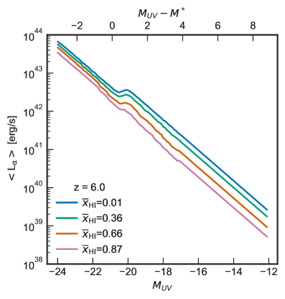
Figure 3: Expectation value for Ly$\alpha$ luminosity at $z=6.0$ for a range of $M_{\textsc{uv}}$ values and $x_{\textsc{hi}}$ values. Here, we also show how $\langle L_{\alpha}\rangle$ compares for galaxies brighter or fainter than ${M_{\textsc{uv}}}^{*}$ (where we use ${M_{\textsc{uv}}}^{*}=-20.9$ at $z=6.0$ from Mason et al., 2015b). The model expects UV-faint galaxies to have an average Ly$\alpha$ luminosity lower than that of UV-bright galaxies. As the neutral fraction increases, $\langle L_{\alpha}\rangle$ decreases. For UV-bright galaxies, there is not much decrease in the Ly$\alpha$ luminosity expected (a factor of $\sim 2$), compared to a factor $\sim 10$ for UV-faint galaxies. The bump in the plot, around ${M_{\textsc{uv}}}\sim-20$, is due to the EW probability distribution threshold between UV-bright and UV-faint galaxies (see Mason et al., 2018), and is discussed further in Section 3.1.

Figure 3 shows a decrease in Ly$\alpha$ luminosity for a given $M_{\textsc{uv}}$ as $x_{\textsc{hi}}$ increases, as expected due to the reduced transmission in an increasingly neutral IGM (Mason et al., 2018). This effect is strongest for UV-faint galaxies, where the average Ly$\alpha$ luminosity decreases by a factor of $\sim 10$ as $x_{\textsc{hi}}$ increases to 1. UV-bright galaxies do not show much decrease in Ly$\alpha$ luminosity at different $x_{\textsc{hi}}$ . The more sizeable impact of reionization on UV-faint galaxies is because they typically exist in the outskirts of dense IGM environments. Thus, a more neutral IGM shifts their Ly$\alpha$ luminosity towards even lower values.

The bump in the plot, around ${M_{\textsc{uv}}}\sim-20$, is due to the EW probability distribution threshold between UV-bright and UV-faint galaxies (Mason et al., 2018). We tested the importance of this bump by fixing the $P(EW)$ distribution (in our case we tested at $P(EW|{M_{\textsc{uv}}})=P(EW|{M_{\textsc{uv}}}=-17)$) which removes the bump. However, this drastically affected the Ly$\alpha$ LF model where it does not fit observations well on the bright-end. This means that $P(EW)$ must be shifted to lower EW values for galaxies brighter than ${M_{\textsc{uv}}}<-20$.

3.2 Evolution of the Ly$\alpha$  luminosity function

We compare our model Ly$\alpha$ LF to observations at $z=5.7,6.6,7.0,7.3$. In Figure 4, we plot our Ly$\alpha$ LF models for a range of $x_{\textsc{hi}}$ from a fully neutral to fully ionized IGM at a given redshift. We also plot observations by Ouchi et al. (2008, 2010); Shibuya et al. (2012); Konno et al. (2014); Santos et al. (2016); Ota et al. (2017); Konno et al. (2018); Itoh et al. (2018); Hu et al. (2019); Taylor et al. (2020) for comparison. Note that we use the selection incompleteness un-corrected LFs by Hu et al. (2019) for the best comparison with other observations and our model, which is calibrated using data which do not account for this incompleteness. Our simple model reproduces the shape of the Ly$\alpha$ LF remarkably well. Note that our Ly$\alpha$ LF is slightly lower than the one observed by Santos et al. (2016). This mismatch between their Ly$\alpha$ LF and other works found in literature is known and discussed, e.g., in Taylor et al. (2020); Hu et al. (2019).

We see that at $z=5.7,6.6,7.0$ the observations are fairly consistent with ${x_{\textsc{hi}}}\sim 0.15-0.36$, whereas at $z=7.3$ the data are more consistent with ${x_{\textsc{hi}}}\sim 0.66-0.87$, suggesting an increasingly neutral IGM environment as redshift increases, consistent with other observations at $z\sim 7$ (e.g., Mason et al., 2018; Whitler et al., 2020; Mason et al., 2019b; Hoag et al., 2019).

Our model predicts that there is not much decrease in number density at low neutral fractions, ${x_{\textsc{hi}}}\,\hbox to0.0pt{\lower 3.5pt\hbox{$\mathchar 0\relax\sim$}\hss}\raise 1.0pt\hbox{$<$}\,0.4$ but the LF decreases more rapidly at higher neutral fractions. Based on Figure 3 the lack of evolution at ${x_{\textsc{hi}}}\,\hbox to0.0pt{\lower 3.5pt\hbox{$\mathchar 0\relax\sim$}\hss}\raise 1.0pt\hbox{$<$}\,40\%$ can be explained by the fact that the bright-end of the Ly$\alpha$ LF is dominated by UV-bright galaxies which exist in over-dense regions of IGM that tend to reionize early (Mesinger & Furlanetto, 2007; Mesinger, 2016; Harikane et al., 2018). Thus, only in reionization’s earliest stages do these galaxies experience significant reduction in transmission.

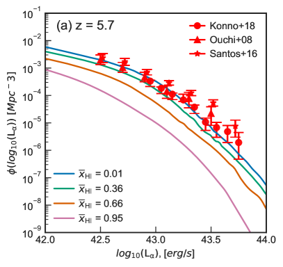
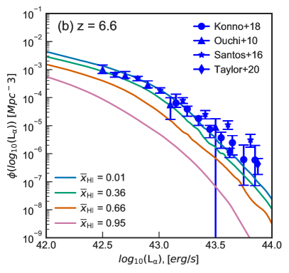
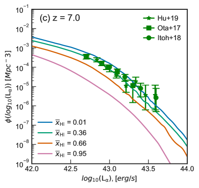
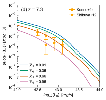
Figure 4: Our predictions for Ly$\alpha$ LF for $z=5.7,6.6,7.0,7.3$ at ${x_{\textsc{hi}}}=0.01-0.87$ (explained in Section 3.2). We also plot observations by Ouchi et al. (2008, 2010); Shibuya et al. (2012); Konno et al. (2014); Santos et al. (2016); Ota et al. (2017); Konno et al. (2018); Itoh et al. (2018); Hu et al. (2019); Taylor et al. (2020) for comparison with our model. Each model line corresponds to a different neutral fraction. The Ly$\alpha$ LF model decreases and changes shape at each redshift as $x_{\textsc{hi}}$ increases. By comparing the observations to our model, as redshift increases, an increasingly neutral IGM is favoured.

3.3 Evolution of Schechter function parameters for the Ly$\alpha$ LF

We fit Schechter parameters, $\alpha,L^{*},\phi^{*}$, for our models using emcee (Foreman-Mackey et al., 2013) to predict how the shape of the Ly$\alpha$ LF evolves with redshift and neutral fraction. To compare with observations, we fit the LF over the luminosity range $42.5<\log_{10}L_{\alpha}/\mathrm{erg\,s}^{-1}<44$. We fit the Schechter function to our Ly$\alpha$ LF models with all possible combinations of redshift and $x_{\textsc{hi}}$ but point out that the resulting Ly$\alpha$ LF are not exact Schechter functions for realistic Ly$\alpha$ EW distributions (even if the input UV LF is) – our Ly$\alpha$ LFs are generally less steep at the bright-end than a Schechter function. Further details about the fitting are provided in Appendix A.

In Figure 5 we plot the evolution of each parameter (where we show the median value from the fits) with respect to redshift and $x_{\textsc{hi}}$ . We see that the parameters decrease overall as the universe becomes more neutral due to Ly$\alpha$ photon attenuation and decrease with redshift because galaxies become fainter and rarer as redshift increases (as seen in the UV LF (Figure 2)).

The left panel of Figure 5 shows redshift versus $\alpha$, which is the power law slope for very low luminosities. At fixed $x_{\textsc{hi}}$ , $\alpha$ decreases as redshift increases, within the slope range of approximately $-2.5<\alpha<-1.8$, as expected due the hierarchical build-up of galaxies producing an increasingly steep faint-end slope of the UV LF with redshift (Mason et al., 2015b). The points plotted at each redshift show the impact of neutral hydrogen. $\alpha$ decreases significantly more due to the neutral gas than it does with redshift because Ly$\alpha$ attenuation affects faint galaxies more and thus makes them fainter, forcing them further back into the Ly$\alpha$ LF.

The center panel of Figure 5 reveals that $L^{*}$ decreases in the range $z=5-7$, but increases sharply toward $z=8$, and declines toward higher redshifts at fixed neutral fractions. This upturn is a consequence of the evolving shape of the UV LF due to dust attenuation at these redshifts in our model. In Mason et al. (2015b), there is an overlapping between $z=6-8$ for the UV LF model around ${M_{\textsc{uv}}}=-23$ which corresponds to $L_{\alpha}=10^{43.6}\,\mathrm{erg\,s}^{-1}$, also seen in observations (e.g., Bouwens et al., 2016, 2015). This overlapping is consistent with a reduction in dust obscuration, such that younger, brighter galaxies at higher redshifts contain less dust and so, there is a possibility of observing more of them and shifting the LF models towards higher luminosities. As the neutral fraction increases at each redshift, the characteristic Ly$\alpha$ luminosity, $L^{*}$, decreases. This trend can be attributed to an increasing attenuation of Ly$\alpha$ photons from UV-bright galaxies as the neutral fraction increases.

The right panel of Figure 5 shows a decreasing number density of Ly$\alpha$ emitting galaxies as we look back to higher redshifts. For each redshift, as shown, assuming the IGM is ionized, more Ly$\alpha$ emitting galaxies are expected to be visible to us and thus the number density increases with decreasing redshift, compared to a neutral IGM. At higher redshifts and at a fixed neutral fraction, we see an overall decrease in number density of Ly$\alpha$ emitters – due to the overall reduction in the number of galaxies at high redshifts (as seen in the evolution of the UV LF, e.g., Bouwens et al., 2015, 2016; Mason et al., 2015b).

We did not compare our Schechter function parameters directly with observations as previous works used a fixed $\alpha$ to determine their best-fit Schechter function parameters (e.g, Konno et al., 2014, 2018; Ouchi et al., 2008, 2010; Itoh et al., 2018; Ota et al., 2017; Hu et al., 2019). As the Schechter function parameters are degenerate (see, e.g., discussion in Herenz et al., 2019), it is difficult to compare with our model directly. Also note that our model for the Ly$\alpha$ LF is not well described by a Schechter fit – our model LFs are typically less steep at the bright end than a Schechter function’s exponential drop-off (see Figure 9). In our approach (Equation 2) we do not expect the Ly$\alpha$ LF to be Schechter form as the integral of the Schechter UV LF does not have a Schechter form, as discussed in Section 3.1 of Gronke et al. (2015). Physical reasons for an observed bright-end excess in the Ly$\alpha$ LF are discussed in Section 4.1 of Konno et al. (2018), including the contribution of AGN, large ionized bubbles around bright LAEs and gravitational lensing.

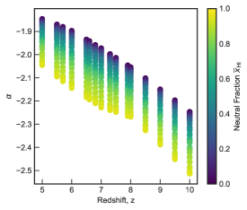
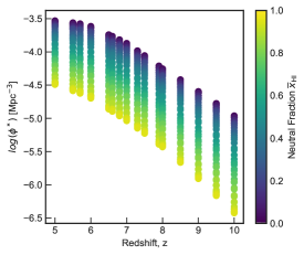
Figure 5: The evolution of the Schechter function parameters $\alpha,L^{*},\phi^{*}$ (left, center, right panels respectively), as a function of redshift $z=5-10$ with a step of $\Delta z=0.5$. Models at different average neutral fractions, $x_{\textsc{hi}}$ are shown with different colors referenced on the adjacent colorbar. Further details about the fitting procedure are explained in Sections 3.3 and Appendix A. We find strong evolution of the Schechter function parameters with $x_{\textsc{hi}}$ , in which each parameter decreases as the neutral fraction increases because Ly$\alpha$ photons become more attenuated.

3.4 Evolution of Ly$\alpha$ luminosity density

The Ly$\alpha$ luminosity density (LD) is the total energy emitted in Ly$\alpha$ by all galaxies obtained by integrating the luminosity function:

$$\rho_{\alpha}(z,{x_{\textsc{hi}}})=\int L_{\alpha}\phi(L_{\alpha},z,{x_{\textsc{hi}}})\,\mathrm{d}L_{\alpha}$$ (16)

where $\phi(L_{\alpha},z,{x_{\textsc{hi}}})$ is our Ly$\alpha$ LF model number density. We generate $\rho_{\alpha}(z,{x_{\textsc{hi}}})$ from our model by integrating over our luminosity grid $10^{42.4}\leq L_{\alpha}\leq 10^{44.5}$ erg s^-1 to compare with observations that use similar luminosity limits, as the luminosity density is highly sensitive to the minimum luminosity, due to the power-law slope of the LF faint end.

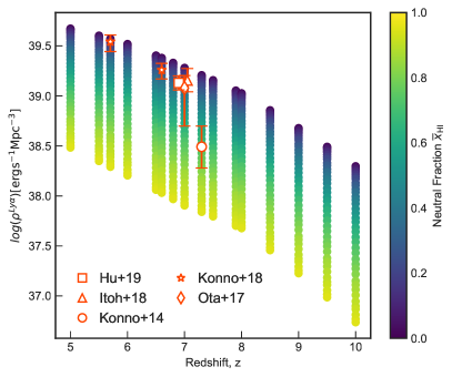
Figure 6: Evolution of the Ly$\alpha$ luminosity density as a function of redshift and the IGM neutral fraction between $z=5-10$. Observational data from Konno et al. (2018) (orange stars, $z=5.7,6.6$), Hu et al. (2019) (orange squares, $z=6.9$), Itoh et al. (2018) (orange triangles, $z=7.0$), Ota et al. (2017) (orange diamonds, $z=7.0$) and Konno et al. (2014) (orange circles, $z=7.3$), show a clear drop in the overall Ly$\alpha$ luminosity density as redshift increases. The LD model shows a decreasing trend as redshift increases and we can expect to see lower LD values as the neutral fraction increases at any redshift.

Figure 6 shows the evolution of the luminosity density along a range of redshifts, $z=5-10$, and the neutral fraction, $x_{\textsc{hi}}$ , predicted by our model. The modelled luminosity density decreases by a factor of $\sim 10$ as the universe becomes more neutral and declines overall as redshift increases. Observations from Konno et al. (2014, 2018); Hu et al. (2019); Itoh et al. (2018); Ota et al. (2017) at $z=5.7,6.6,7.0,7.3$ show a decrease in luminosity density to higher redshifts. We compare our model with observations and see that the LD observations are consistent with a mostly ionized IGM at $z=5.7,6.6,7.0$ and increase towards a more neutral IGM at $z=7.3$. These observations, similar to the Ly$\alpha$ LF observations, are chosen based on their selection incompleteness being un-corrected further explained in Hu et al. (2019). We also chose to plot Ly$\alpha$ LD observations that were considered fiducial (some works also tested separate LD points at different $\alpha$ to compare with others).

3.5 The evolution of the neutral fraction at $z>6$

We perform a Bayesian inference for the neutral fraction based on our model, as explained in Section 2.4. We infer ${x_{\textsc{hi}}}$ at $z=6.6,7.0,7.3$ by fitting our model to LF observations by Shibuya et al. (2012); Konno et al. (2014, 2018); Itoh et al. (2018); Ota et al. (2017); Hu et al. (2019). We infer ${x_{\textsc{hi}}}(z=6.6)=0.08^{+0.08}_{-0.05},\,{x_{\textsc{hi}}}(z=7.0)=0.28\pm 0.05$ and ${x_{\textsc{hi}}}(z=7.3)=0.83^{+0.06}_{-0.07}$ (all errors are $1\sigma$ credible intervals). Appendix B shows the posterior distributions for $x_{\textsc{hi}}$ at each redshift (Figure 10).

We also show the comparisons between the posterior distributions for the neutral fraction obtained using the Ly$\alpha$ LD observations (Konno et al., 2014; Ota et al., 2017; Konno et al., 2018; Itoh et al., 2018; Hu et al., 2019, see Section 3.4). As expected, we see larger uncertainties in the estimations of the neutral fraction from the Ly$\alpha$ LD data due to including fewer data points compared to the LFs. We find ${x_{\textsc{hi}}}(z=6.6)=0.22^{+0.12}_{-0.11}$, ${x_{\textsc{hi}}}(z=7.0)=0.25\pm 0.08$, and ${x_{\textsc{hi}}}(z=7.3)=0.69^{+0.12}_{-0.11}$. Using the full LF data thus not only enables us to infer neutral fractions that are more robust to non-uniform Ly$\alpha$ transmission, but adds a statistical advantage over previous luminosity density methods by reducing the uncertainty on the neutral fraction (for further discussion, we refer the reader to Section 4.2).

Figure 7 shows our new constraints on reionzation history along with other approaches to estimating the neutral fraction. Our results show clear upward trend in neutral fraction at higher redshifts, consistent with an IGM that reionizes fairly rapidly. Our measurement at $z=6.6$ is consistent with previous upper limits on the neutral fraction at $z\leq 6.6$ (McGreer et al., 2015; Ouchi et al., 2010; Sobacchi & Mesinger, 2015). Our measurement at $z=7.0$ is consistent with inferences from the Ly$\alpha$ damping wing in the quasar ULAS J1120+0641 (Davies et al., 2018), but is lower than than constraints from the Ly$\alpha$ EW distribution in LBGs by (Mason et al., 2018; Whitler et al., 2020), though is still consistent within $2\sigma$. Our measurement at $z=7.3$ is consistent with other constraints at $z>7$ (Hoag et al., 2019; Mason et al., 2019b; Davies et al., 2018) though, like the other $z>7$ constraints, is higher than the QSO damping wing measurements at $z=7.5$ for the quasar ULAS J1342+0928 by Greig et al. (2019).

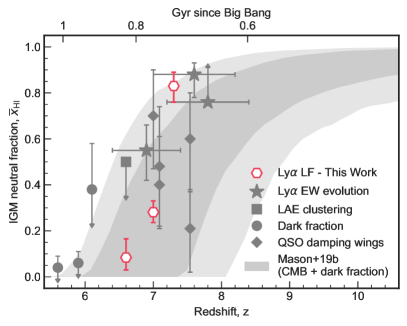
Figure 7: IGM neutral fraction of hydrogen as a function of redshift updated from Mason et al. (2018). Reionization history plot with this work corresponding to the Ly$\alpha$ LF given a $1\sigma$ uncertainty (red hexagons). Constraints derived from observations of previous estimates from the fraction of LBGs emitting Ly$\alpha$ are plotted (star; Mason et al. (2018, 2019b); Whitler et al. (2020); Hoag et al. (2019)); the clustering of Ly$\alpha$ emitting galaxies (square; Ouchi et al. (2010); Sobacchi & Mesinger (2015)); Ly$\alpha$ and Ly$\beta$ forest dark fraction (circle; McGreer et al. (2015)); and QSO damping wings (diamond; Greig & Mesinger (2017); Davies et al. (2018); Greig et al. (2019); Wang et al. (2020)). The shaded regions of the reionization plot show the corresponding $1\sigma$ and $2\sigma$ uncertainty coverage consistent with Planck Collaboration et al. (2016) $\tau$ and dark fraction (Mason et al., 2019a).

3.6 Predictions for Nancy Grace Roman Space Telescope, Euclid and JWST surveys

The Nancy Grace Roman Space Telescope High Latitude Survey (NGRST HLS) and the Euclid Deep Field Survey (DFS) will both be particularly important surveys which will probe into higher redshifts and detect Ly$\alpha$ emission lines further into the Epoch of Reionization with wide-area slit-less spectroscopy. The James Webb Space Telescope (JWST) will also be able to detect high redshift Ly$\alpha$ with high sensitivity, albeit in smaller areas. Here we make predictions for potential Ly$\alpha$ LFs with these telescopes.

The Euclid Deep Field Survey will cover a 40 sq. degree area at a $5\sigma$ flux limit of $\sim 8.6\times 10^{-17}$ erg s^-1 cm^-2. It will cover $0.9\leq\lambda_{\mathrm{obs}}\leq 1.3\mu$m corresponding to a redshift range for Ly$\alpha$ of $6\leq z\leq 10$ (e.g, Laureijs et al., 2012; Bagley et al., 2017). NGRST High Latitude Survey will cover $1.00\leq\lambda_{\mathrm{obs}}\leq 1.95\mu$m corresponding to a redshift range for Ly$\alpha$ of $8\leq z\leq 15$, and survey a 2200 sq. degree area at a $5\sigma$ flux limit of $\sim 7.1\times 10^{-17}$ erg s^-1 cm^-2 (e.g, Ryan et al., 2019; Spergel et al., 2013). JWST’s slit-less spectrograph NIRISS will cover $0.7\leq\lambda_{\mathrm{obs}}\leq 5.0\mu$m, capable of detecting Ly$\alpha$ at $z\gtrsim 5$. While there is no dedicated wide-area survey with NIRISS, we investigate a mock pure-parallel survey of 50 pointings ($\sim 240$ sq. arcmin) with a $5\sigma$ flux limit of $\sim 5.0\times 10^{-18}$ erg s^-1 cm^-2, assuming 2 hour exposures with the F115W filter.

We make predictions for these surveys in Figure 8. We plot our model Ly$\alpha$ LF and the approximate median neutral fraction value based the reionization history allowed by the CMB optical depth and dark pixel fraction at each redshift (Mason et al., 2019a) between $6<z<10$ (shown as the gray shaded region in Figure 7). We see that these surveys will detect luminous Ly$\alpha$ emitters at higher redshifts. We predict the NGRST HLS will be able to discover galaxies $L_{\alpha}>10^{43.76}$ erg s^-1 at redshifts up to $z=10$. Euclid Deep Field survey will be able to detect bright galaxies at $L_{\alpha}>10^{43.84}$ erg s^-1 but only up to $z\sim 8$. Using the JWST mock pure-parallel survey, we estimate it be able to detect bright galaxies at $L_{\alpha}>10^{42.61}$ erg s^-1 up to $z\sim 9-10$.

We note that the predicted number counts will likely be higher than shown in Figure 8 due to gravitational lensing magnification bias, which can increase the observed number of galaxies at the bright-end of the LF in flux-limited surveys (Wyithe et al., 2011; Mason et al., 2015a; Marchetti et al., 2017).

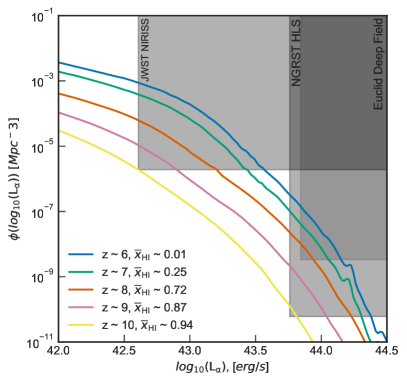
Figure 8: Ly$\alpha$ LF model at redshifts $z=6-10$ and their corresponding median neutral fraction values. The shaded boxes represent the survey depth coverage for the NGRST High Latitude Survey (a $5\sigma$ flux limit of $\sim 7.1\times 10^{-17}$ erg s^-1 cm^-2 and a redshift range of $8\leq z\leq 15$ (e.g, Ryan et al., 2019; Spergel et al., 2013), the Euclid Deep Field Survey (a $5\sigma$ flux limit of $\sim 8.6\times 10^{-17}$ erg s^-1cm^-2 and a redshift range of $6\leq z\leq 10$ (e.g, Laureijs et al., 2012; Bagley et al., 2017), and the JWST NIRISS mock pure-parallel survey (a $5\sigma$ flux limit of $\sim 5.0\times 10^{-18}$ erg s^-1 cm^-2 and a redshift range of $z\gtrsim 5$). We calculate the luminosity limits and depths for the NGRST HLS, Euclid DFS, and JWST NIRISS mock pure-parallel survey at a median redshift value of $z=8$.

4 Discussion

In this Section, we discuss uncertainties that affect our Ly$\alpha$ LF model (Section 4.1), a comparison with previous work that attempted to constrain reionization from Ly$\alpha$ LFs (Section 4.2), and an explanation of our Ly$\alpha$ luminosity distributions for both Ly$\alpha$ and UV-selected galaxies and their affect on the normalization factor (Section 4.3).

4.1 Modelling caveats

In building our model, we make several assumptions that can affect the results which are summarized here. These assumptions are also described by Mason et al. (2018); Whitler et al. (2020) and we refer the reader there for additional details. Firstly, we assume that the intrinsic ‘emitted’ Ly$\alpha$ luminosity distribution does not evolve with redshift (only $M_{\textsc{uv}}$ ) and is the same as the observed Ly$\alpha$ luminosity distribution at $z\sim 6$ (as modelled from the EW distribution by Mason et al., 2018), and that only evolution in the ‘observed’ luminosity distribution is due to reionization alone. However, we should expect some evolution in the Ly$\alpha$ luminosity distribution with redshift, as galaxy properties evolve. Physically, we could expect galaxies to have higher luminosities as redshift increases, due to, e.g., lower dust attenuation (Hayes et al., 2011), which leads to a steepening of the Ly$\alpha$ LF with redshift (Gronke et al., 2015; Dressler et al., 2015). In that case, more significant absorption by the IGM would be required to explain the observed Ly$\alpha$ LFs and we would thus infer a higher inferred neutral fraction. Alternatively, a decrease in outflow velocities possibly associated with a decreasing specific SFR, could lower Ly$\alpha$ escape from galaxies, decreasing the emitted luminosity (Hassan & Gronke, 2020), in which case a lower neutral fraction would be inferred.

We also assume that Ly$\alpha$ visibility evolution between $z=6-7$ is due only to the evolution of the Ly$\alpha$ damping wing optical depth (e.g., Miralda-Escudé, 1998), due to the diffuse neutral IGM. We do not model redshift evolution of the Ly$\alpha$ transmission in the ionized IGM or CGM at fixed halo mass (e.g., Laursen et al., 2011; Weinberger et al., 2018). The amount of transmission due to these components is determined by the Ly$\alpha$ line shape. If the Ly$\alpha$ line velocity offset from systemic decreases with redshift at fixed halo mass, this would decrease the Ly$\alpha$ transmission throughout the ionized IGM and CGM (Dijkstra et al., 2011; Choudhury et al., 2015) and reduce the need for a highly neutral IGM. A full exploration of the degeneracies and systematic uncertainties due to the Ly$\alpha$ emission model is left to future work.

4.2 Comparison with previous work

In this work we directly compare measurements of the Ly$\alpha$ LF to our model. Previous works, e.g. Ouchi et al. (2010); Zheng et al. (2017); Konno et al. (2014, 2018); Inoue et al. (2018); Hu et al. (2019), estimate the neutral fraction by evaluating the Ly$\alpha$ luminosity density. While this provides a reasonable first-order estimate, this method can be difficult to interpret as it relies on models and observations using the same luminosity limit in the luminosity density integral, and it collapses any valuable information that is obtained in the evolving shape of the Ly$\alpha$ LF (including increasing the statistical uncertainty on $x_{\textsc{hi}}$ by reducing the number of data points – see Appendix B). As demonstrated in Section 3.3 the Ly$\alpha$ shape does evolve.

Furthermore, these works estimate the neutral fraction based on the assumption that the transmission fraction, $T_{\mathrm{IGM}}$ is constant for all galaxies. However, as shown by e.g. Mason et al. (2018); Whitler et al. (2020) it is a broad distribution and depends on galaxy properties, through their large scale structure environment and the internal kinematics that sets the Ly$\alpha$ line shape. If the transmission fraction varies with Ly$\alpha$ or UV luminosity, the common method of calculating Ly$\alpha$ transmission by taking the ratio of the Ly$\alpha$ luminosity density at different redshifts is invalid, thus our work enables a more robust estimate of $x_{\textsc{hi}}$ from the Ly$\alpha$ LFs. Many of these works compare with simulations by McQuinn et al. (2007), which do model the impact of inhomogeneous reionization on the Ly$\alpha$ LF but take a more simplistic approach to modelling Ly$\alpha$ luminosity: each galaxy has a Ly$\alpha$ luminosity proportional to its mass. In our work, we use the EW probability distribution from Mason et al. (2015b), to take into account that galaxies have a range of Ly$\alpha$ EW at fixed UV magnitude. Our approach is thus more similar to that of Jensen et al. (2013) who model the Ly$\alpha$ luminosity probability distribution as a function of halo mass. However, Jensen et al. (2013) model the Ly$\alpha$ luminosity and equivalent width distributions independently, whereas we have shown the Ly$\alpha$ LF can be self-consistently described by the same Ly$\alpha$ EW distribution that describes Lyman-break galaxies.

Finally, our semi-analytic model provides flexibility over approaches which model radiative transfer in N-body simulations (e.g., Dayal et al., 2011; Jensen et al., 2013; Hutter et al., 2014; Inoue et al., 2018) or sophisticated hydrodynamical simulations (e.g., Dayal et al., 2011; Weinberger et al., 2019), by keeping the IGM neutral fraction and redshift as free parameters, rather than assuming a fixed reionization history. Using this new model for the Ly$\alpha$ LF, we can separate redshift and the neutral fraction, fixing either parameter if needed, and see how observations compare to our model.

4.3 Reconciling the Ly$\alpha$ luminosity distributions for Ly$\alpha$ and UV-selected galaxies

As described in Section 2.3, a normalization factor, $F$, is introduced to the Ly$\alpha$ LF to account for any mismatch in the number density of LAEs (Dijkstra & Wyithe, 2012). If the Ly$\alpha$ luminosity distribution model accurately describes the Lyman-break galaxy population observed in the UV LF, we expect $F=1$. We find $F=0.974$ in our model, which is considerably higher than previous work focusing on the Ly$\alpha$ LF at lower redshifts which found $F\sim 0.5$ (Dijkstra & Wyithe, 2012; Gronke et al., 2015).

The key difference compared to this previous work which leads to our model successfully reproducing the Ly$\alpha$ LF without the need for additional normalization, is due to the EW distribution we employed. While we, as well as the previous work, include non-emitters in the model, the EW distribution used by Dijkstra & Wyithe (2012); Gronke et al. (2015) (calibrated to measurements of Shapley et al., 2003; Stark et al., 2010; Stark et al., 2011, at $z\sim 3-6$) shows an increasing probability of Ly$\alpha$ emission for lower UV brightness galaxies, leading to a Ly$\alpha$ emitter ($EW>0$ Å) fraction of unity for ${M_{\textsc{uv}}}\,\hbox to0.0pt{\lower 3.5pt\hbox{$\mathchar 0\relax\sim$}\hss}\raise 1.0pt\hbox{$>$}\,-19$. The EW distribution we used caps this ‘emitter fraction’ at $65\%$ (our function $A({M_{\textsc{uv}}})$ in Section 2.1.1).

Which parametrization of the EW distribution is most appropriate is still up to debate (see, e.g., detailed discussion by Oyarzún et al., 2017, who study more complex distributions also dependent on the stellar mass and the UV slope). The recent study of Caruana et al. (2018) supports our non-emitter fraction, as they find a fraction of $\sim 0.5\pm 0.15$ galaxies with $EW>0\,$Å at $3<z<6$ in HST continuum selected galaxies for within the MUSE Wide field (Herenz et al., 2017; Urrutia et al., 2019) is present. However, Caruana et al. (2018) also find a non-evolution of this fraction with UV magnitude (in contrast with previous models) as well as typically lower Ly$\alpha$ fractions for larger EW cuts (e.g., the value for $W>50\,$Å seems to be in slight tension with measurements by Stark et al., 2010 who find $\approx 45\pm 10\%$ of galaxies have Ly$\alpha$ $EW>55\,$Å and a strong anti-correlation with UV brightness).

Another factor to consider when comparing $z\lesssim 3$ and $z\gtrsim 5$ EW distributions is the impact of the IGM on the Ly$\alpha$ line even at $z\sim 5-6$. In fact, is has been suggested by Weinberger et al. (2019) that $F$ could stem from this effect but note that Dijkstra & Wyithe (2012) and Gronke et al. (2015) compare their modelled Ly$\alpha$ LFs at $z\sim 3$ to data by Ouchi et al. (2008); Gronwall et al. (2007) and Rauch et al. (2008), respectively, and still require $F\sim 0.5$ at this low $z$.

Future observational studies will constrain the Ly$\alpha$ EW distribution further both as a function of redshift and UV magnitude, and thus can quantify the fraction of non-emitters for UV faint galaxies. We have shown that a constant non-emitter fraction of $\sim 35\%$ for $M_{\rm UV}\lesssim-19$ makes the fudge factor $F\sim 0.5$ obsolete, which indicates that such a ‘cutoff’ exists in reality.

5 Conclusions

We have developed a model for the Ly$\alpha$ LF during reionization, and compared it with observations at specific redshifts to estimate the evolution of the neutral fraction. Our model can be extended to predict the evolution of the Ly$\alpha$ LF with neutral fraction at even higher redshifts, deeper in the era of reionization. Our model takes into account inhomogeneous reionization, enabling us to understand the impact of galaxy environment on the Ly$\alpha$ LF.

Our conclusions are as follows:

1. By combining previously established models for the UV luminosity function and the Ly$\alpha$ EW distribution for UV-selected galaxies, we successfully reproduce the observed $z=5.7$ Ly$\alpha$ luminosity function (derived from Ly$\alpha$ -selected galaxies).

2. Our model predicts a decline in the Ly$\alpha$ luminosity function as the neutral fraction increases. For ${x_{\textsc{hi}}}\,\hbox to0.0pt{\lower 3.5pt\hbox{$\mathchar 0\relax\sim$}\hss}\raise 1.0pt\hbox{$<$}\,0.4$, the Ly$\alpha$ LF models exhibit relatively little decrease in number density, however, at higher neutral fractions we see a significant drop in number density.

3. We predict that the average Ly$\alpha$ luminosity for a Lyman-break galaxy of a given UV magnitude decreases as the neutral fraction increases. We find there is only a moderate decrease in Ly$\alpha$ luminosity for UV-bright galaxies at increasing $x_{\textsc{hi}}$ (factor of $\sim 2$ from a fully ionized to fully neutral IGM), because they typically exist in dense regions of the universe that reionize early, allowing large amounts of Ly$\alpha$ photons to be transmitted. For UV-faint galaxies which are typically found in neutral IGM regions, we see a decrease in Ly$\alpha$ luminosity by a factor of $\sim 10$ with the neutral fraction.

4. We find strong evolution of the Schechter function parameters with $x_{\textsc{hi}}$ , demonstrating the LF shape changes. The faint-end slope $\alpha$, number density $\phi^{*}$ and the characteristic luminosity $L^{*}$ all generally decrease with increasing neutral fraction. These decreases in the Schechter function parameters with increasing $x_{\textsc{hi}}$ can be explained by a reduction in Ly$\alpha$ luminosity from all galaxies, with the faintest galaxies experiencing the most significant decline in transmission which shifts the faint-end slope to steeper values.

5. The Ly$\alpha$ luminosity density decreases overall as the universe becomes more neutral, as shown by previous work.

6. We perform a Bayesian inference of the IGM neutral fraction given observations using our model. We infer an IGM neutral fraction at $z=6.6$ of ${x_{\textsc{hi}}}=0.08^{+0.08}_{-0.05}$, rising to ${x_{\textsc{hi}}}=0.28\pm 0.05$ for $z=7.0$ and ${x_{\textsc{hi}}}=0.83^{+0.06}_{-0.07}$ for $z=7.3$, providing further evidence for a late and fairly rapid reionization.

7. Using our Ly$\alpha$ LF model with a fiducial reionization history, we predict the NGRST HLS will be able to discover bright galaxies with $L_{\alpha}>10^{43.76}$ erg s^-1 at redshifts up to $z=10$. Euclid Deep Field survey will be able to detect bright galaxies at $L_{\alpha}>10^{43.84}$ erg s^-1 but only up to $z\sim 8$. Using a JWST mock pure-parallel survey, we estimate it be able to detect galaxies at $L_{\alpha}>10^{42.61}$ erg s^-1 up to $z\sim 9-10$.

Constraining the evolving shape of the Ly$\alpha$ LF as a function of redshift provides an important tool to estimate the evolving neutral fraction during reionization. Understanding the timeline of reionization and the properties of galaxies that existed as a function of redshift, and how they are impacted by neutral gas, can ultimately be used to infer properties of the first stars and galaxies that initialized reionization.

Appendix A Example of fitting Schechter function parameters

Figure 9 shows examples of outputs for the best-fit Schechter function parameters for $z=5.7$ and ${x_{\textsc{hi}}}=0.01$ as described in Section 3.3. We perform a Bayesian inference (Equation 11) to obtain the parameters, using the likelihood:

$$P(\phi\,|\,\alpha,L_{\star},\phi_{\star})\propto\prod_{i}\exp{\left[-\left(\ln{\phi_{\mathrm{mod}}(L_{i})}-\ln{\phi_{\mathrm{Sch}}(L_{i},\alpha,L_{\star},\phi_{\star})}\right)^{2}\right]}$$ (A1)

where $\phi_{\mathrm{mod}}(L_{i})$ are our model Ly$\alpha$ LFs at luminosity values $L_{i}$, and $\phi_{\mathrm{Sch}}(L_{i},\alpha,L_{\star},\phi_{\star})$ is the Schechter function (Equation 1). We perform the inference using emcee (Foreman-Mackey et al., 2013).

For all Schechter function fits, we restrict the fit to the luminosity range $41.0<\log_{10}L_{\alpha}<44.0$ erg s^-1, and use the following uniform priors for the Bayesian inference: $-4<\alpha<0$, $40<\log_{10}L_{\star}<44$ and $-10<\log_{10}\phi_{\star}<-2$. Example posteriors and fitted LFs are shown in Figure 9. We explored a variety of luminosity ranges for the fitting and note that the absolute values of the recovered Schechter parameters are quite sensitive to the fitted luminosity range, however the trends in redshift and neutral fraction are consistent across the luminosity ranges, as long as $<L_{\star}$ luminosities were included. Our model LFs have $L_{\star}\sim 10^{43}$ erg s^-1, comparable to the luminosity limits of $z\,\hbox to0.0pt{\lower 3.5pt\hbox{$\mathchar 0\relax\sim$}\hss}\raise 1.0pt\hbox{$>$}\,7$ surveys (e.g., Ota et al., 2017; Hu et al., 2019), demonstrating the importance of deep LAE surveys to obtain accurate fits to the observed luminosity functions. In our analysis in Section 3.3 we use the use the median values of the Schechter function parameters obtained from the posteriors. Note that our model for the Ly$\alpha$ LF is not well described by a Schechter fit – we see a shallower bright-end drop off.

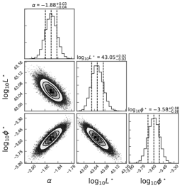
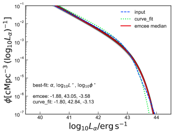
Figure 9: (Left) Posterior probability distributions for Schechter function parameters fit to our Ly$\alpha$ LF model at $z=5.7$ and ${x_{\textsc{hi}}}=0.01$. (Right) Our Ly$\alpha$ LF model at $z=5.7$ and ${x_{\textsc{hi}}}=0.01$ (blue dashed line) compared with the best-fit Schechter functions. Thin black solid lines show Schechter LFs with parameters from 100 draws from the posterior distribution. The Schechter LF obtained from the median of the posteriors is shown as the red solid line. We also plot the Schechter fit obtained using SciPy curve_fit for comparison (green dotted line). We use the median values of the Schechter function parameters for our analysis.

Appendix B Inference of the neutral fraction, $x_{\textsc{hi}}$ at $z=6.6,7.0,7.3$

To infer the neutral fraction we calculate a posterior distribution for $z=6.6,7.0,7.3$. The posterior, defined in Section 2.4, is normalized and plotted against neutral fraction values ${x_{\textsc{hi}}}$. To determine the $68\%$ and $95\%$ confidence intervals, we interpolate the inverse cumulative distribution function (CDF) to find the neutral fraction value that falls at a given confidence interval value. Figure 10 shows the $x_{\textsc{hi}}$ posterior at each redshift for both Ly$\alpha$ LF data and Ly$\alpha$ LD data, along with the confidence intervals. We also compare the Ly$\alpha$ LF models at the median $x_{\textsc{hi}}$ values to the data to verify our inferred values.

To verify advantages the Ly$\alpha$ LF may have over the Ly$\alpha$ LD in estimating the median neutral fraction, we establish the $x_{\textsc{hi}}$ posterior using the Ly$\alpha$ LD data. We expect larger uncertainties in the neutral fraction using only the LD data – the errors should roughly increase by $\sqrt{N}$, where $N$ is the ratio of the number of individual data points with the two methods. Also note, some observations do not have Ly$\alpha$ LD data that can be included in the estimation of the neutral fraction (e.g, Ouchi et al., 2010; Shibuya et al., 2012) and thus also affect the results.

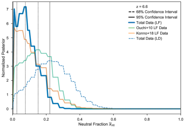
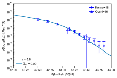
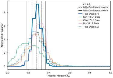
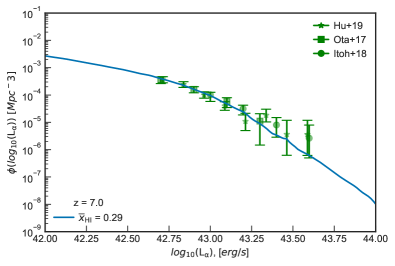
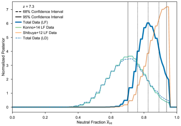
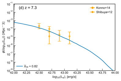
Figure 10: (Left) Neutral hydrogen fraction versus the normalized posterior distribution $P({x_{\textsc{hi}}}|\phi_{\mathrm{obs}},z)$ (see Section 2.4) for each redshift. The thick blue lines in each posterior plot show the total posterior distributions at each redshift alongside the individual posterior distributions for each data set (shown in either green, orange, or pink thin lines). The blue dashed lines correspond to total Ly$\alpha$ LD posterior distributions. The black dashed lines show the $68\%$ or $1\sigma$ confidence interval where the upper, lower, and median limits are defined. The black solid lines show the upper and lower limits for the $95\%$ or $2\sigma$ confidence interval. For redshifts $z=6.6,7.0,7.3$, our median neutral fraction values (mid-dashed line on the left figures) is estimated to be: ${x_{\textsc{hi}}}(z=6.6)=0.08$, ${x_{\textsc{hi}}}(z=7.0)=0.28$, and ${x_{\textsc{hi}}}(z=7.3)=0.83$. If we compare our total data posteriors, the Ly$\alpha$ LD posterior distribution has median neutral fraction values of: ${x_{\textsc{hi}}}(z=6.6)=0.22$, ${x_{\textsc{hi}}}(z=7.0)=0.25$, and ${x_{\textsc{hi}}}(z=7.3)=0.69$. In Figure 7 we plot the median and $68\%$ confidence interval values. (Right) We show the corresponding Ly$\alpha$ LF plot at that redshift and median neutral fraction value to verify our fit.

References

- Ando et al. (2006) Ando M., Ohta K., Iwata I., Akiyama M., Aoki K., Tamura N., 2006, ApJ, 645, L9
- Atek et al. (2015) Atek H., et al., 2015, ApJ, 814, 69
- Bañados et al. (2018) Bañados E., et al., 2018, Nature, 553, 473
- Bagley et al. (2017) Bagley M. B., et al., 2017, ApJ, 837, 11
- Barkana & Loeb (2007) Barkana R., Loeb A., 2007, Reports on Progress in Physics, 70, 627
- Bouwens et al. (2014) Bouwens R. J., et al., 2014, ApJ, 793, 115
- Bouwens et al. (2015) Bouwens R. J., et al., 2015, ApJ, 803, 34
- Bouwens et al. (2016) Bouwens R. J., et al., 2016, ApJ, 830, 67
- Bowler et al. (2015) Bowler R. A. A., et al., 2015, MNRAS, 452, 1817
- Caruana et al. (2018) Caruana J., et al., 2018, MNRAS, 473, 30
- Choudhury et al. (2015) Choudhury T. R., Puchwein E., Haehnelt M. G., Bolton J. S., 2015, MNRAS, 452, 261
- Ciardi et al. (2003) Ciardi B., Stoehr F., White S. D. M., 2003, MNRAS, 343, 1101
- Clément et al. (2012) Clément B., et al., 2012, A&A, 538, A66
- Dahlen et al. (2005) Dahlen T., Mobasher B., Somerville R. S., Moustakas L. A., Dickinson M., Ferguson H. C., Giavalisco M., 2005, The Astrophysical Journal, 631, 126
- Davies et al. (2018) Davies F. B., et al., 2018, ApJ, 864, 142
- Dayal & Ferrara (2018) Dayal P., Ferrara A., 2018, Phys. Rep., 780, 1
- Dayal et al. (2011) Dayal P., Maselli A., Ferrara A., 2011, MNRAS, 410, 830
- De Barros et al. (2017) De Barros S., et al., 2017, A&A, 608, A123
- Dijkstra & Wyithe (2012) Dijkstra M., Wyithe J. S. B., 2012, Monthly Notices of the Royal Astronomical Society, 419, 3181
- Dijkstra et al. (2011) Dijkstra M., Mesinger A., Wyithe J. S. B., 2011, MNRAS, 414, 2139
- Dressler et al. (2015) Dressler A., Henry A., Martin C. L., Sawicki M., McCarthy P., Villaneuva E., 2015, ApJ, 806, 19
- Fan et al. (2006) Fan X., Carilli C., Keating B., 2006, Annual Review of Astronomy and Astrophysics, 44, 415
- Finkelstein et al. (2015a) Finkelstein S. L., et al., 2015a, ApJ, 810, 71
- Finkelstein et al. (2015b) Finkelstein S. L., et al., 2015b, ApJ, 810, 71
- Finkelstein et al. (2019) Finkelstein S. L., et al., 2019, ApJ, 879, 36
- Foreman-Mackey et al. (2013) Foreman-Mackey D., Hogg D. W., Lang D., Goodman J., 2013, PASP, 125, 306
- Furlanetto & Oh (2005) Furlanetto S. R., Oh S. P., 2005, MNRAS, 363, 1031
- Gillet et al. (2020) Gillet N. J. F., Mesinger A., Park J., 2020, MNRAS, 491, 1980
- Greig & Mesinger (2017) Greig B., Mesinger A., 2017, MNRAS, 465, 4838
- Greig et al. (2017) Greig B., Mesinger A., Haiman Z., Simcoe R. A., 2017, MNRAS, 466, 4239
- Greig et al. (2019) Greig B., Mesinger A., Bañados E., 2019, MNRAS, 484, 5094
- Gronke et al. (2015) Gronke M., Dijkstra M., Trenti M., Wyithe S., 2015, Monthly Notices of the Royal Astronomical Society, 449, 1284–1290
- Gronwall et al. (2007) Gronwall C., et al., 2007, ApJ, 667, 79
- Harikane et al. (2018) Harikane Y., et al., 2018, PASJ, 70, S11
- Hashimoto et al. (2017) Hashimoto T., et al., 2017, A&A, 608, A10
- Hassan & Gronke (2020) Hassan S., Gronke M., 2020, arXiv e-prints, p. arXiv:2010.00023
- Hayes et al. (2011) Hayes M., Schaerer D., Östlin G., Mas-Hesse J. M., Atek H., Kunth D., 2011, ApJ, 730, 8
- Herenz et al. (2017) Herenz E. C., et al., 2017, A&A, 606, A12
- Herenz et al. (2019) Herenz E. C., et al., 2019, A&A, 621, A107
- Hibon et al. (2010) Hibon P., et al., 2010, A&A, 515, A97
- Hoag et al. (2019) Hoag A., et al., 2019, ApJ, 878, 12
- Hu et al. (2019) Hu W., et al., 2019, ApJ, 886, 90
- Hunter (2007) Hunter J. D., 2007, Comput. Sci. Eng., 9, 99
- Hutter et al. (2014) Hutter A., Dayal P., Partl A. M., Müller V., 2014, MNRAS, 441, 2861
- Inoue et al. (2018) Inoue A. K., et al., 2018, PASJ, 70, 55
- Itoh et al. (2018) Itoh R., et al., 2018, ApJ, 867, 46
- Jensen et al. (2013) Jensen H., Laursen P., Mellema G., Iliev I. T., Sommer-Larsen J., Shapiro P. R., 2013, MNRAS, 428, 1366
- Jung et al. (2018) Jung I., et al., 2018, ApJ, 864, 103
- Jung et al. (2020) Jung I., et al., 2020, arXiv e-prints, p. arXiv:2009.10092
- Kelly et al. (2008) Kelly B. C., Fan X., Vestergaard M., 2008, ApJ, 682, 874
- Konno et al. (2014) Konno A., et al., 2014, ApJ, 797, 16
- Konno et al. (2016) Konno A., Ouchi M., Nakajima K., Duval F., Kusakabe H., Ono Y., Shimasaku K., 2016, ApJ, 823, 20
- Konno et al. (2018) Konno A., et al., 2018, PASJ, 70, S16
- Krug et al. (2012) Krug H. B., et al., 2012, ApJ, 745, 122
- Larson et al. (2018) Larson R. L., et al., 2018, The Astrophysical Journal, 858, 94
- Laureijs et al. (2012) Laureijs R., et al., 2012, in Clampin M. C., Fazio G. G., MacEwen H. A., Oschmann Jacobus M. J., eds, Society of Photo-Optical Instrumentation Engineers (SPIE) Conference Series Vol. 8442, Space Telescopes and Instrumentation 2012: Optical, Infrared, and Millimeter Wave. p. 84420T, doi:10.1117/12.926496
- Laursen et al. (2011) Laursen P., Sommer-Larsen J., Razoumov A. O., 2011, ApJ, 728, 52
- Malhotra & Rhoads (2004) Malhotra S., Rhoads J. E., 2004, ApJ, 617, L5
- Marchetti et al. (2017) Marchetti L., Serjeant S., Vaccari M., 2017, MNRAS, 470, 5007
- Mason et al. (2015a) Mason C. A., et al., 2015a, ApJ, 805, 79
- Mason et al. (2015b) Mason C. A., Trenti M., Treu T., 2015b, ApJ, 813, 21
- Mason et al. (2018) Mason C. A., Treu T., Dijkstra M., Mesinger A., Trenti M., Pentericci L., de Barros S., Vanzella E., 2018, ApJ, 856, 2
- Mason et al. (2019a) Mason C. A., et al., 2019a, MNRAS, 485, 3947
- Mason et al. (2019b) Mason C. A., et al., 2019b, Monthly Notices of the Royal Astronomical Society, 485, 3947
- Matthee et al. (2014) Matthee J. J. A., et al., 2014, MNRAS, 440, 2375
- McGreer et al. (2015) McGreer I. D., Mesinger A., D’Odorico V., 2015, MNRAS, 447, 499
- McQuinn et al. (2007) McQuinn M., Hernquist L., Zaldarriaga M., Dutta S., 2007, MNRAS, 381, 75
- Mesinger (2016) Mesinger A., 2016, Understanding the Epoch of Cosmic Reionization. Vol. 423, doi:10.1007/978-3-319-21957-8,
- Mesinger & Furlanetto (2007) Mesinger A., Furlanetto S., 2007, ApJ, 669, 663
- Mesinger et al. (2014) Mesinger A., Aykutalp A., Vanzella E., Pentericci L., Ferrara A., Dijkstra M., 2014, Monthly Notices of the Royal Astronomical Society, 446, 566
- Miralda-Escudé (1998) Miralda-Escudé J., 1998, ApJ, 501, 15
- Miralda-Escudé et al. (2000) Miralda-Escudé J., Haehnelt M., Rees M. J., 2000, ApJ, 530, 1
- Mirocha et al. (2020) Mirocha J., Mason C., Stark D. P., 2020, MNRAS, 498, 2645
- Morishita et al. (2018) Morishita T., et al., 2018, ApJ, 867, 150
- Naidu et al. (2020) Naidu R. P., Tacchella S., Mason C. A., Bose S., Oesch P. A., Conroy C., 2020, ApJ, 892, 109
- Oesch et al. (2013) Oesch P. A., et al., 2013, ApJ, 773, 75
- Oesch et al. (2015) Oesch P. A., et al., 2015, ApJ, 804, L30
- Oesch et al. (2018) Oesch P. A., et al., 2018, ApJS, 237, 12
- Oliphant (2007) Oliphant T. E., 2007, Comput. Sci. Eng., 9, 10
- Ota et al. (2008) Ota K., et al., 2008, ApJ, 677, 12
- Ota et al. (2010) Ota K., et al., 2010, ApJ, 722, 803
- Ota et al. (2017) Ota K., et al., 2017, ApJ, 844, 85
- Ouchi et al. (2008) Ouchi M., et al., 2008, ApJS, 176, 301
- Ouchi et al. (2010) Ouchi M., et al., 2010, ApJ, 723, 869
- Oyarzún et al. (2017) Oyarzún G. A., Blanc G. A., González V., Mateo M., Bailey John I. I., 2017, ApJ, 843, 133
- Partridge & Peebles (1967) Partridge R. B., Peebles P. J. E., 1967, ApJ, 147, 868
- Pérez & Granger (2007) Pérez F., Granger B. E., 2007, Comput. Sci. Eng., 9, 21
- Planck Collaboration et al. (2016) Planck Collaboration et al., 2016, A&A, 594, A13
- Rauch et al. (2008) Rauch M., et al., 2008, ApJ, 681, 856
- Rhoads & Malhotra (2001) Rhoads J. E., Malhotra S., 2001, ApJ, 563, L5
- Robitaille et al. (2013) Robitaille T. P., et al., 2013, A&A, 558, A33
- Ryan et al. (2019) Ryan R., et al., 2019, BAAS, 51, 413
- Santos et al. (2016) Santos S., Sobral D., Matthee J., 2016, MNRAS, 463, 1678
- Schechter (1976) Schechter P., 1976, ApJ, 203, 297
- Schenker et al. (2014) Schenker M. A., Ellis R. S., Konidaris N. P., Stark D. P., 2014, ApJ, 795, 20
- Schmidt et al. (2014) Schmidt K. B., et al., 2014, ApJ, 786, 57
- Shapley et al. (2003) Shapley A. E., Steidel C. C., Pettini M., Adelberger K. L., 2003, ApJ, 588, 65
- Shibuya et al. (2012) Shibuya T., Kashikawa N., Ota K., Iye M., Ouchi M., Furusawa H., Shimasaku K., Hattori T., 2012, ApJ, 752, 114
- Shibuya et al. (2018) Shibuya T., et al., 2018, PASJ, 70, S14
- Sobacchi & Mesinger (2015) Sobacchi E., Mesinger A., 2015, MNRAS, 453, 1843
- Spergel et al. (2013) Spergel D., et al., 2013, arXiv e-prints, p. arXiv:1305.5425
- Stark et al. (2010) Stark D. P., Ellis R. S., Chiu K., Ouchi M., Bunker A., 2010, MNRAS, 408, 1628
- Stark et al. (2011) Stark D. P., Ellis R. S., Ouchi M., 2011, ApJ, 728, L2
- Stern et al. (2005) Stern D., Yost S. A., Eckart M. E., Harrison F. A., Helfand D. J., Djorgovski S. G., Malhotra S., Rhoads J. E., 2005, ApJ, 619, 12
- Tacchella et al. (2013) Tacchella S., Trenti M., Carollo C. M., 2013, ApJ, 768, L37
- Tacchella et al. (2018) Tacchella S., Bose S., Conroy C., Eisenstein D. J., Johnson B. D., 2018, ApJ, 868, 92
- Taylor et al. (2020) Taylor A. J., Barger A. J., Cowie L. L., Hu E. M., Songaila A., 2020, ApJ, 895, 132
- Tilvi et al. (2010) Tilvi V., et al., 2010, ApJ, 721, 1853
- Tilvi et al. (2016) Tilvi V., et al., 2016, ApJ, 827, L14
- Trenti & Stiavelli (2008) Trenti M., Stiavelli M., 2008, ApJ, 676, 767
- Trenti et al. (2010) Trenti M., Stiavelli M., Bouwens R. J., Oesch P., Shull J. M., Illingworth G. D., Bradley L. D., Carollo C. M., 2010, ApJ, 714, L202
- Treu et al. (2013) Treu T., Schmidt K. B., Trenti M., Bradley L. D., Stiavelli M., 2013, ApJ, 775, L29
- Urrutia et al. (2019) Urrutia T., et al., 2019, A&A, 624, A141
- Van Der Walt et al. (2011) Van Der Walt S., Colbert S. C., Varoquaux G., 2011, Comput. Sci. Eng., 13, 22
- Wang et al. (2020) Wang F., et al., 2020, ApJ, 896, 23
- Weinberger et al. (2018) Weinberger L. H., Kulkarni G., Haehnelt M. G., Choudhury T. R., Puchwein E., 2018, MNRAS, 479, 2564
- Weinberger et al. (2019) Weinberger L. H., Haehnelt M. G., Kulkarni G., 2019, MNRAS, 485, 1350
- Whitler et al. (2020) Whitler L. R., Mason C. A., Ren K., Dijkstra M., Mesinger A., Pentericci L., Trenti M., Treu T., 2020, MNRAS, 495, 3602
- Wyithe et al. (2011) Wyithe J. S. B., Yan H., Windhorst R. A., Mao S., 2011, Nature, 469, 181
- Zheng et al. (2017) Zheng Z.-Y., et al., 2017, ApJ, 842, L22