The rapid transition from star-formation to AGN dominated rest-frame UV light at $\mathbf{z\simeq 4}$

Abstract

With the advent of deep optical-to-near-infrared extragalactic imaging on the degree scale, samples of high-redshift sources are being selected that contain both bright star-forming (SF) galaxies and faint active galactic nuclei (AGN). In this study we investigate the transition between SF and AGN-dominated systems at $z\simeq 4$ in the rest-frame UV. We find a rapid transition to AGN-dominated sources bright-ward of $M_{\rm UV}\simeq-23.2$. The effect is observed in the rest-frame UV morphology and size-luminosity relation, where extended clumpy systems become point-source dominated, and also in the available spectra for the sample. These results allow us to derive the rest-frame UV luminosity function for the SF and AGN-dominated sub-samples. We find the SF-dominated LF is best fit with a double-power law, with a lensed Schechter function being unable to explain the existence of extremely luminous SF galaxies at $M_{\rm UV}\simeq-23.5$. If we identify AGN-dominated sources according to a point-source morphology criterion we recover the relatively flat faint-end slope of the AGN LF determined in previous studies. If we instead separate the LF according to the current spectroscopic AGN fraction, we find a steeper faint-end slope of $\alpha=-1.83\pm 0.11$. Using a simple model to predict the rest-frame AGN LF from the $z=4$ galaxy LF we find that the increasing impact of host galaxy light on the measured morphology of faint AGN can explain our observations.

1 Introduction

How supermassive black holes and their host galaxies co-evolve over cosmic time poses many fundamental questions within Astrophysics. The detection of luminous quasars at very high redshift (e.g. Fan et al., 2003; Willott et al., 2010a; Mortlock et al., 2011; Bañados et al., 2016, 2018; Yang et al., 2020) demonstrates that active black holes are present less than a Gyr after the Big Bang. Within the same epoch, the star-forming (SF) galaxy population is known to be building-up rapidly from measurements of the evolving rest-frame UV luminosity function (LF; e.g. Bouwens et al., 2015; Finkelstein et al., 2015; Bowler et al., 2020; Ono et al., 2018). Until recently, the populations of quasars and SF galaxies at redshifts $z=4-8$ have typically been treated as separate, due primarily to the disparate luminosity space occupied by the current samples. This is despite the majority of galaxies and quasars at very high-redshifts being selected based on the same spectral feature in optical/NIR survey data; the Lyman-continuum and/or the Lyman-$\alpha$ break. The strong Lyman-break in the spectral energy distribution (SED), which is redshifted into the optical filters at $z\gtrsim 3$ and near-IR at $z\gtrsim 7$, has allowed large samples of UV-bright galaxies and AGN to be selected efficiently. In the last decade, the advent of intermediate surveys that probe areas up to a few hundred square degrees on the sky has led to the first samples that bridge both faint AGN as well as bright galaxies, filling in a previously unachievable parameter space in volume and luminosity (Matute et al., 2013; Kashikawa et al., 2015; Matsuoka et al., 2018b; Stevans et al., 2018; Ono et al., 2018; Adams et al., 2020). The properties of these intermediate luminosity sources are important for several reasons. Firstly, the existence of very UV bright, highly star-forming galaxies can challenge models of feedback and dust obscuration via the inferred steepness of the bright-end of the Lyman-break galaxy (LBG) UV LF (e.g. Bower et al., 2012; Gonzalez-Perez et al., 2013; Bowler et al., 2014; Dayal et al., 2014; Clay et al., 2015). Furthermore, the uncertainty in the number of the brightest galaxies in combination with ‘contamination’ of these samples with faint-AGN or interloper populations can confuse the interpretation of the shape and evolution of the galaxy LF (e.g. Bowler et al., 2012; Bian et al., 2013). Secondly, the determination of the faint-end slope of the AGN LF is crucial for understanding if these sources played any significant role in reionizing the Universe at $z\gtrsim 7$ (e.g. as advocated by Giallongo et al., 2015, 2019, see discussion in Parsa et al., 2018). Thirdly, samples of sources in which the AGN and stellar component both contribute measurably to the observed light give an insight into how and when black holes become intricately linked to their host galaxy (e.g. via measurements of the black-hole to bulge/stellar mass relation at very high-redshift; Willott et al., 2010b; Venemans et al., 2017).

While the rest-frame UV $z\simeq 4$ AGN LF was first measured several decades ago (e.g. Warren et al., 1994; Richards et al., 2006; Masters et al., 2012; Ikeda et al., 2012), recent surveys have been able to select larger samples over a wider luminosity range, thus providing greater precision. In particular, there have been several successful campaigns to identify fainter sources at $z\geq 4$ with surveys such as the Subaru High-$z$ Exploration of Low-Luminosity Quasars (SHELLQs: Matsuoka et al., 2018a), the Infrared Medium Survey (IMS: Kim et al., 2019) and the Hyper-SuprimeCam Stragetic Survey Program (HSC-SSP; Akiyama et al., 2018). These studies have been able to constrain the faint-end of the AGN LF for the first time at $z\gtrsim 4$, however there remain large discrepancies in the derived faint-end slope which ranges from $\alpha\simeq-1.3$ (Matsuoka et al., 2018b; Akiyama et al., 2018) to as steep as $\alpha\simeq-2$ (McGreer et al., 2018; Giallongo et al., 2019; Shin et al., 2020). A key challenge in the robust determination of the number density of the lowest luminosity AGN is that faint-ward of a certain absolute UV magnitude ($M_{\rm UV}\simeq-23$; Stevans et al., 2018; Ono et al., 2018; Adams et al., 2020), LBGs become overwhelmingly more numerous. In response, AGN selection methodologies have typically included a condition that the source must be unresolved in imaging data, as expected for a source dominated by the central AGN. Despite this, the very faintest sources targeted by these studies have shown spectra that are typical of Lyman-break galaxies (e.g. Matsuoka et al., 2018b; Kashikawa et al., 2015). Furthermore, as studies probe fainter AGN in the rest-frame UV, it is unclear how the light from star-formation might impact the morphology (e.g. Gavignaud et al., 2006) and hence cause current selection procedures based on compactness to become incomplete. Thus a more detailed analysis of the properties of faint-AGN and bright galaxies is required.

In Adams et al. (2020) we selected a sample of LBGs and AGN at $z\simeq 4$ from the COSMOS and XMM-LSS deep extragalactic fields using a photometric redshift analysis based on the ground-based optical to NIR photometry. The advantages of this sample over previous studies are i) we do not impose any condition on source size or morphology and hence we are complete to both point-sources and extended galaxies, ii) we exploit the NIR data which results in a very clean selection of $z\simeq 4$ sources and iii) we have used two of the most widely studied deep fields where there is wealth of deep multi-wavelength data and spectroscopy available. Here we utilise this sample to investigate the properties of objects within the ‘transition’ regime between bright-AGN and the typical galaxy population at this redshift. We do this by looking at the morphology and size of the sources using both the available ground-based and wide-area Hubble Space Telescope (HST) mosaics in COSMOS. In addition we have compiled publicly available spectra for the sample and use this to further classify sources. The structure of the paper is as follows. In Section 2 we describe the variety of datasets we use, and in Section 3 we describe the size measurements and the results from the available archival spectra of the sample. In Section 4 we derive the AGN fraction from our data and estimate the separated SF and AGN-dominated LFs. We discuss our results in 5 and present a simple empirical model of the AGN LF which we use to interpret our results in Section 6. We end with conclusions in 7. Throughout this work we present magnitudes in the AB system (Oke, 1974; Oke & Gunn, 1983). The standard concordance cosmology is assumed, with $H_{0}=70\,{\rm km}\,{\rm s}^{-1}\,{\rm Mpc}^{-1}$, $\Omega_{\rm m}=0.3$ and $\Omega_{\Lambda}=0.7$. At $z=[3.5,4.0,4.5]$ this cosmology implies that one arcsec corresponds to physical distances of $[7.3,7.0,6.6]\,{\rm kpc}$.

2 Sample selection and data

The sample of $z\simeq 4$ galaxies and AGN we utilize in this work was selected in the COSMOS and XMM-LSS deep extragalactic fields. The selection was based on a photometric redshift fitting of the optical to NIR bands (u-band to $K_{s}$) from the available ground-based data. In this paper we further include HST ACS imaging and spectroscopic observations available in the public domain.

2.1 The sample

The full sample of $z\simeq 4$ sources from Adams et al. (2020) consisted of 20064 (38722) sources in the COSMOS (XMM-LSS) fields bright-ward of the 50 percent completeness limit of $M_{\rm UV}\simeq-20$. To be included in the sample the object must have a best-fitting photometric redshift in the range $3.5<z<4.5$ with either a galaxy or AGN SED. Stars were removed using a relative $\chi^{2}$ cut, such that the galaxy or AGN template must have a better fit than the stellar model. In this work we refined this sample using the most up-to-date photometry in the fields. We matched the original catalogue with a new $I$-band selected catalogue (created in an identical fashion) that included the deeper HSC DR2 data, and the UltraVISTA DR4 imaging. The matching process revealed a small number of artefacts that were removed in the newer HSC release. We also required the objects to satisfy the selection criterion described above when run on the new deeper photometry, and be brighter than $15\sigma$ in the ground-based $I$-band to ensure a robust morphology analysis. As a result of these steps we were left with a sample of 15126 (25592) sources in COSMOS (XMM-LSS). For the morphology analysis we required the sources to be covered by the HST/ACS mosaic in the COSMOS field. The sub-sample covered by this mosaic contained 13848 sources.

2.2 Imaging data

Within the COSMOS field we used the HST/Advanced Camera for Surveys (ACS) mosaic in the F814W filter (hereafter $I_{814}$: Koekemoer et al., 2007; Scoville et al., 2007; Massey et al., 2010). We obtained $10\times 10\,{\rm arcsec}^{2}$ cut-outs from this mosaic for each source in our COSMOS sample where the ACS data existed (corresponding to 96 percent of the sample). The ACS data has a pixel scale of $0.03\,{\rm arcsec}/{\rm pix}$, and a typical point-source full-width-at-half-maximum (FWHM) of less than 0.1 arcsec. The COSMOS field is uniformly covered to single orbit depth, leading to a $5\sigma$ depth of 27.0 (0.6 arcsecond diameter aperture). Both the COSMOS and XMM-LSS fields contain a wealth of data in the optical and NIR bands. In this study we measure the rest-frame UV size from the HSC $I$ and CFHT $i$-bands. This allowed us to identify any potential systematics in the size measurement from using data of different depth and seeing. The HSC $I$-band is available across both fields, with varying depth, while the CFHT $i$-band is uniform in depth but is available for only a 1$\,{\rm deg}^{2}$ subsection of each field (Bowler et al., 2020). The images have a pixel scale of $0.15$ and $0.2$ in COSMOS and XMM-LSS respectively. The seeing in these bands was approximately 0.65 arcsec.

2.3 Publicly available spectroscopy

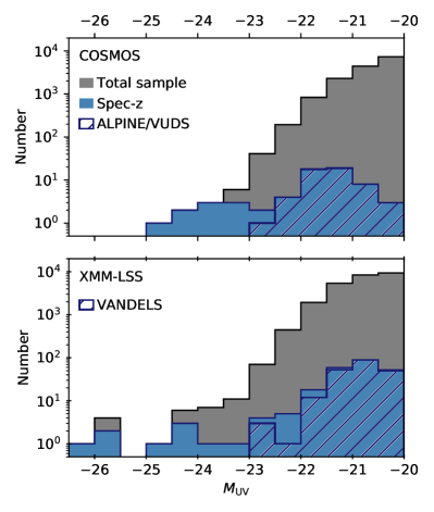
Figure 1: The absolute UV magnitude distribution of our sample of $z\simeq 4$ sources selected initially in Adams et al. (2020). The samples in the COSMOS and XMM-LSS fields are shown in the upper and lower plots respectively. The total sample of galaxies and AGN with best-fit photometric redshifts in the range $3.5<z<4.5$ are shown as the grey histogram. The spectroscopically confirmed sources are shown as the blue shaded histogram. In hatched blue we have highlighted the spectroscopic redshifts from the deep galaxy surveys of ALPINE and VUDS in COSMOS and VANDELS in XMM-LSS. The spectroscopic redshifts at brighter magnitudes are typically from magnitude limited surveys (e.g. SDSS, zCOSMOS; see Table 2).

We endeavoured to extract the publicly available spectroscopy for the sample. In both fields we initially matched to the compilation of spectroscopic redshifts created by the HSC team, which we supplemented with additional catalogues from the VANDELS (Pentericci et al., 2018; McLure et al., 2018) in XMM-LSS, and the ALMA Large Program to INvestigate (ALPINE; Fèvre et al., 2019) and the Boutsia et al. (2018) sample of $z\simeq 4$ AGN in COSMOS. In Fig. 1 we show the spectroscopically confirmed sources in comparison to the full sample as a function of absolute UV magnitude. In total we found a total of 63 and 236 high-redshift sources with secure spectroscopic flags in COSMOS and XMM-LSS respectively (76 and 270 with all flags). As part of this process we identified and removed 4 (12) low-redshift interlopers in COSMOS (XMM-LSS). In COSMOS, 100 percent of the sources in our sample at $M_{\rm UV}<-23.5$ are confirmed spectroscopically, partially due to the campaign of Boutsia et al. (2018). In XMM, we find a lower percentage of 42 percent in the same magnitude range. At the bright-end of our sample the spectroscopic redshifts come primarily from magnitude limited surveys including the Sloan Digital Sky Survey (SDSS; Eisenstein et al., 2011; Richards et al., 2002), zCOSMOS (Lilly et al., 2007), VIMOS VLT Deep Survey (VVDS; Le Fèvre et al., 2015) and Primus (Coil et al., 2011). At the faint-end of our survey the redshifts were obtained as specific follow-up for high-redshift galaxies. The ALPINE sample includes sources from the VIMOS Ultra Deep Survey (VUDS; Le Fèvre et al., 2015) and Deep Imaging Multi-Object Spectrograph (DEIMOS; Hasinger et al., 2018) follow-up of high-redshift sources that are spread over the COSMOS field. The VANDELS survey on the other hand, was limited to a smaller region of the field that overlaps with the HST Cosmic Assembly NIR Deep Extragalactic Legacy Survey (CANDELS; Grogin et al., 2011; Koekemoer et al., 2011) where extremely deep spectroscopic integrations were performed. Thus the VANDELS sources extend to fainter magnitudes than in ALPINE. At the faint-end of the survey $\lesssim 2$ percent of our sample have been confirmed as part of these deep spectroscopic surveys. While we cross-matched our sample to all available spectroscopic redshifts, we were only able to obtain a subset of reduced spectra depending on the survey. We extracted all of the publicly available spectra from SDSS, zCOSMOS, VVDS and VANDELS for further analysis.

3 Results

Armed with our sample of $z\simeq 4$ sources in the COSMOS and XMM-LSS fields, we proceeded to measure their sizes and spectroscopic properties. As we are primarily concerned with the objects in the ‘transition’ regime where AGN and LBGs have similar number densities, this analysis focuses on the results at $M_{\rm UV}\lesssim-22$. At these bright magnitudes we have a larger proportion of spectroscopic follow-up from magnitude limited surveys and we are able to identify the source morphology at high S/N in the high-resolution HST data (e.g. even if the source fragments into several clumps the components are detected individually at $>5\,\sigma$).

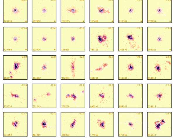
Figure 2: Postage-stamp images in the HSC/ACS $I_{814}$ band of the brightest 30 sources in our COSMOS $z\simeq 4$ sample. The sources are presented in order of $M_{\rm UV}$, with the brightest sources in the top left, spanning the range $-24.18<M_{\rm UV}<-22.67$. The stamps are $2\,{\rm arcsec}$ on a side (corresponding to $\sim 14\,{\rm kpc}$ at $z=4$), in the standard orientation of North to the top, and East to the left. The images have been scaled by surface brightness, from $2\sigma$ (approximately $24{\rm mag}/{\rm arcsec}$) to the peak. Contours have been added at intervals of $1{\rm mag}$ starting at the peak, to highlight the central compactness of the sources. The ID number is shown in the bottom left and the $M_{\rm UV}$ is shown in the upper right. Sources that have been spectroscopically confirmed are labelled with an astericks in the bottom right corner. Note that all of the spectroscopically confirmed sources in this figure show strong quasar features in the spectra.

3.1 Visual morphology

We first visually inspected the $z\simeq 4$ sources that had high-resolution imaging from the COSMOS HST/ACS $I_{814}$ mosaic. In Fig. 2 we show postage-stamp images of the brightest 30 sources in our sample. The brightest eight sources have been spectroscopically confirmed as quasars (see Table 2) and as expected, these sources appear compact. As we go fainter in this sub-sample there is a dramatic change in the visual morphology, with the appearance of extended, clumpy, sources. For example objects ID793151, ID746876 and ID168777 are clearly resolved, with multiple-components that extend $>0.5\,{\rm arcsec}$ ($>3.5\,{\rm kpc}$) from the centroid. This is as expected from the galaxy size-luminosity relation and extensive studies of similarly luminous sources at $z\simeq 3$ (e.g. Law et al., 2012; Lotz et al., 2006) and $z>5$ (e.g. Jiang et al., 2013; Bowler et al., 2017). In the sources that are confirmed as AGN from their spectra, there is some evidence for weak extended emission (e.g. ID702265), which could be arising from the host galaxy. Furthermore, one of the sources (ID153468) that is a confirmed quasar from the available rest-frame UV spectrum in Boutsia et al. (2018), appears to be compact but resolved (which is also confirmed by quantitative measure of the size, see Section 4.1). This demonstrates that the host galaxy light is contributing significantly to the rest-frame UV light from this source. We estimated the contribution from the host galaxy by simultaneously fitting a PSF and Sérsic profile (fixed to $n=1.0$; Law et al., 2012) to the image using GALFIT. The best-fit from this crude estimate was an equal contribution from the AGN and SF in this object. For the other visual point-sources in the data, we found that a PSF alone was adequate to fit the imaging. If we assume that the extended sources are SF-dominated, whilst the point-sources are AGN dominated (which is likely given the high rate of AGN spectra found for these sources), then we see a rapid transition in the individual galaxy morphology that indicates a transition from AGN to SF dominated systems at $M_{\rm UV}\simeq-23$. A transition at this magnitude is in good agreement with that predicted by the simultaneous AGN and LBG LF fitting of Adams et al. (2020) and we compare our results directly to this study in our analysis of the AGN fraction in Section 4.1.

3.2 Size-luminosity relation

Due to the clumpy nature of the sources in the HST $I_{814}$ data, the sizes of these sources can be substantially biased depending on the chosen measurement technique. When running Source Extractor (SE; Bertin & Arnouts, 1996) on these images for example, we found that the majority of the SF-dominated sources were de-blended into several component. This results in a severe underestimate of the individual sizes of the brightest galaxies in the sample. To get around this issue we proceeded to make high signal-to-noise stacks of the data over a range in $M_{\rm UV}$.

3.2.1 Stacking procedure

We created stacks in both the high-resolution HST imaging and the ground-based HSC and CFHT $i$-band data. In both cases masks were formed from the SEGMENTATION images created with SE. For the ground-based data we masked all sources that were not associated with the central source. In the HST/ACS data we recombined de-blended components by retaining all objects that were within a radius of 0.8 arcsec from the central coordinate defined by the ground-based centroid. Due to their close proximity, and the extended emission connecting clumps in many cases, we are confident these components are at the same redshift (see Fig. 2 and discussion in Bowler et al., 2017). If the separate components were galaxies at lower redshifts, we would expect these interloper sources to effect the ground-based optical to NIR photometry and thus be removed as interlopers by our SED fitting process. With our recombined source we then determined the new centroid of the detected pixels in this extended object as the barycentre or first order moment (as used in SE). With these masked and centred images we proceeded to stack the images using both an average and median stack for comparison. The size measurement we used was the half-light radius from SE. In the following plots we present the results derived from the median stack using the barycentre centroid, however we comment on any different results found using the other methods. We obtained errors on our stacked size measurements using bootstrap resampling. At the bright-end where there are very few sources in each bin this essentially measures the spread of the individual sizes in that bin.

3.2.2 Results

In Fig. 3 we show the observed sizes of the stack galaxy images, uncorrected for the PSF, as a function of $M_{\rm UV}$ for the ground-based and HST data. At the faint-end of our sample we find that the galaxy stacks are resolved even in the ground-based data, with measured half-light radii in the range $r_{\rm 1/2}\simeq 0.55$–$0.6\,{\rm arcsec}$ as compared to $r_{\rm 1/2}\simeq 0.4$–$0.45\,{\rm arcsec}$ for the PSF. As we move to brighter galaxy stacks there is a gentle increase in size until $M_{\rm UV}\simeq-22.5$, where we see a drop to smaller sizes that are consistent with being unresolved. The results from the HSC $I$-band and the CFHT $i$-band are consistent within the errors for both fields. In COSMOS, where we also have the higher resolution imaging HST $I_{814}$ data, the drop in size observed in the ground-based and HST data occurs at a consistent $M_{\rm UV}$. The wider area covered by XMM-LSS can also explain the shallower decline in size bright-ward of $M_{\rm UV}=-23$ as compared to the COSMOS result, because this larger volume will result in rarer bright galaxies being detected. Indeed, we identify a spectroscopically confirmed galaxy at $M_{\rm UV}=-23.6$ (see Section 3.3). In both COSMOS and XMM-LSS, the brightest sources all appeared as point-source in the ground-based data, however we found that in some cases the measured $r_{1/2}$ was larger than expected due to blending with foreground galaxies.

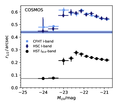
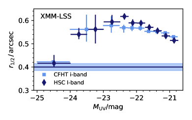
Figure 3: The observed half-light radius of our sample of $z\simeq 4$ sources, uncorrected for the PSF, in the COSMOS and XMM-LSS fields (upper and lower plot respectively). In each plot the dark blue diamonds show the HSC I-band measurement, and the light blue squares show the CFHT i-band result. In the COSMOS plot we show the measured $r_{\rm 1/2}$ from the HSC $I_{814}$-band as the black circles. The blue horizontal band shows the $r_{\rm 1/2}$ measured for the ground-based PSF. The corresponding band for the ACS data is shown as the black/grey line. In all datasets we see a drop off in measured size at $M_{\rm UV}<-22.5$, although this is less pronounced in XMM-LSS.

In order to measure the size-luminosity relation we corrected for the effect of the PSF by subtracting in quadrature the $r_{1/2}$ measured for stars in the imaging. This is an approximate correction for the PSF, however we use it for comparison with previous studies. The size-luminosity relation was measured from the HST/ACS data only, as these data provide the most robust size measurements due to the smaller effect of the PSF (which has $r_{1/2}=0.0725\,{\rm arcsec}$). We then converted the $r_{1/2}$ into a physical distance by assuming a redshift of $z=4.0$. The resulting size-luminosity relation derived from the HST/ACS data is shown in Fig. 4. As expected from this effective rescaling of the observed sizes shown in Fig. 3, we see a clear drop in size at $M_{\rm UV}<-22.5$. To determine the size-luminosity relation from the sample we therefore fit to the points faint-ward of this magnitude, assuming the standard parameterisation of $r_{\rm 1/2}\propto L^{\beta}$ (e.g. Shen et al., 2003). We find a best fitting slope of $\beta=0.16\pm 0.03$, with a normalisation given by $R_{0}=1.45\pm 0.02$ at $M_{\rm UV}=-21.0$. If we use the SE single-component centroid (e.g. prior to recombining de-blended components), we derive an identical slope, but a lower normalisation of $R_{0}=1.36\pm 0.02$. We find no difference in results when using an average stack instead of the median presented here. Our derived size-luminosity relation is consistent with that determined by Huang et al. (2013), who found $\beta=0.22\pm 0.06$, and Curtis-Lake et al., 2016 who found $\beta=0.06\pm 0.11$. We find an offset compared to the relation derived in Curtis-Lake et al. (2016), which we attribute to the different measurement of size used by that study.

By extrapolating our fitted size-luminosity relation to brighter magnitudes, it is evident that there is a dramatic drop in the observed sizes of $z\simeq 4$ sources. We attribute this drop to the increasing contribution of point-sources bright-ward of $M_{\rm UV}=-22.5$, in agreement with the visual morphologies shown in Fig. 2. The transition occurs over almost one magnitude, being complete around $M_{\rm UV}=-23.25$ according to our ACS stacks. From the XMM-LSS results shown in Fig. 3, which cover a wider area than COSMOS and hence are likely to detect the presence of the rarest SF galaxies, there is evidence for extended sources up to $M_{\rm UV}\simeq-24$.

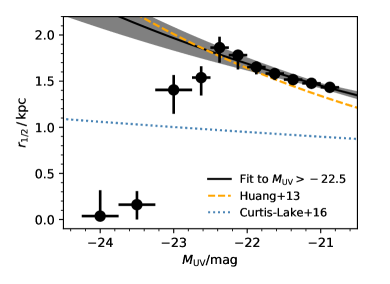
Figure 4: The size-luminosity relation at $z\simeq 4$, derived from the subset of our sample that have high-resolution ACS $I_{814}$ coverage. Our best-fit relation to the points at $M_{\rm UV}>-22.5$ is shown as the solid black line, with the grey shading showing the $1\sigma$ confidence interval. The size-luminosity relation from Huang et al. (2013) and Curtis-Lake et al. (2016) at $z=4$ are shown as the orange dashed and blue dotted lines respectively. A clear deviation from the relation is observed at bright magnitudes, with the sources at $M_{\rm UV}<-23.2$ being consistent with being unresolved by HST/ACS.

3.3 Rest-frame UV spectroscopy

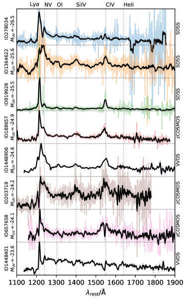
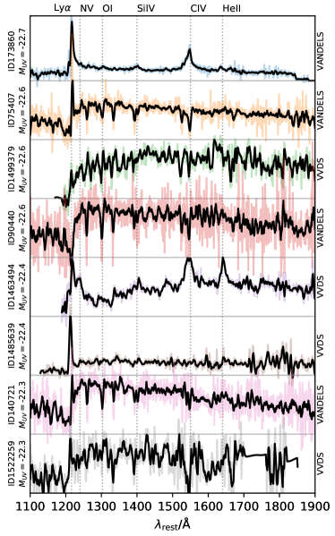
Figure 5: A compilation of rest-frame UV spectra of the brightest sources in the $z\simeq 4$ sample. The spectra have been shifted into the rest-frame according to the spectroscopic redshift provided by each survey, and are ordered by absolute UV magnitude with the brightest source at the top left. The raw data is shown as the coloured background and a box-car filtered spectrum in shown in black. Each spectrum (which was originally in units of ${\rm erg}/{\rm s}/$Å) was normalised to a peak flux of 1.0, and has been presented offset in the vertical direction for clarity. On the left of each spectrum is a label presenting the ID number and the absolute UV magnitude of the object. On the right of each spectrum is the name of the survey which obtained the data. We label common high-ionization emission lines with vertical dashed lines.

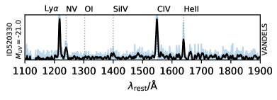
Figure 6: The spectrum of the faintest AGN we have identified in our $z\simeq 4$ sample when cross-matched to publicly available spectra. The data is displayed as in Fig. 5. This source was found within the XMM-LSS field and has a spectrum from the VANDELS survey. It is the only source we find with AGN features faintward of $M_{\rm UV}=-22.4$.

To inform further our classification of sources as SF or AGN-dominated in the ‘transition’ region observed in the size-luminosity relation, we retrieved the publicly available spectra available for the sample. While the brightest sources in our sample are confirmed from magnitude limited surveys (e.g. SDSS, zCOSMOS), there is a dearth of spectra in the range $-23.5<M_{\rm UV}<-22.5$, as is visible in Fig. 1 and shown in Table 2. Nevertheless, we compiled the publicly available spectra and present the results for all sources brighter than $M_{\rm UV}=-22$ in Fig. 5. We smoothed the spectra with a box-car filter of width $1000\,{\rm km}/{\rm s}$ in the rest-frame, to highlight the spectral features above the noise. The brightest seven sources show broad emission lines of NV $\lambda 1240$Å, SiIV $\lambda\lambda 1393,1402$ and CIV$\lambda\lambda 1548,1550$Å in addition to strong Lyman-$\alpha$ emission, all of which are clear signatures of unobscured AGN spectra. In addition to the typical AGN spectra, we identify source that show the appearance of SF-dominated light in the rest-frame UV. Faint-ward of $M_{\rm UV}=-24$ we see a majority of sources that show the appearance of SF-dominated light, with narrow Lyman-$\alpha$ emission and absorption lines. Of particular interest is ID1448401 which is the most luminous source ($M_{\rm UV}=-23.6$) in this sub-sample to show a SF-dominated spectrum. We discuss the implications for the discovery of this object for the LF in Section 4. Within the SF-dominated objects, we see a large variation in the observed spectra, with some showing strong Lyman-$\alpha$ and others showing a continuum break and no appreciable Lyman-$\alpha$ emission.

The sources shown in Fig. 5 are particularly bright which makes it relatively straightforward to see the presence of SF or AGN-type features in the spectra. Even with this limited spectroscopic sub-sample, it is evident that there is a transition in the rest-frame UV spectra of $z\simeq 4$ sources between $-24.0<M_{\rm UV}<-22.0$. Fainter than $M_{\rm UV}=-22.4$ we find only one other spectrum that shows clear evidence of AGN signatures, both through a visual inspection of the smoothed data and through an analysis of the spectral flags provided by each survey. The spectrum of this faint AGN is shown in Fig 6. This source was observed as part of the VANDELS survey of the XMM-LSS field and has $z_{\rm spec}=3.9407$ and $M_{\rm UV}=-21.0$. It lies outside the region of HST data from CANDELS, however it appears extended in the ground-based HSC I-band data, with a PSF uncorrected $r_{\rm 1/2}=0.77\,{\rm arcsec}$. In the spectrum there are again strong emission lines of high-ionization species including CIV and HeII. In comparison to the brighter AGN shown in Fig. 5 however, ID520330 shows stronger and considerably narrower emission lines. We measured the FWHM of the CIV doublet in all of the spectra shown, both directly from the smoothed data and through fitting a simple model of two Gaussians at the doublet wavelengths (constrained to have the same normalisation and standard-deviation). Both methods produced consistent results within the errors. The result of this analysis was that the brighter AGN in our sample show CIV $FWHM\simeq 2000$–$6000\,{\rm km}/{\rm s}$, as found for the general population of SDSS quasars for example (e.g. Vanden Berk et al., 2001). In contrast, the faint source ID520330 shows a significantly narrower width of $FWHM=1200\pm 100\,{\rm km}/{\rm s}$. Similarly, this faint source has the highest rest-frame equivalent width of CIV amongst the AGN spectra, showing $EW_{0}\simeq 150\pm 30$Å. This is to be compared with $EW_{0}\simeq 20$–$90$Å for the brighter sources. Emission lines of this width and strength are characteristic of obscured Type II AGN (e.g. Alexandroff et al., 2013), where only the narrow line region is observed. The fact that we see Type II signatures in the faintest source in the rest-frame UV is also to be expected, as the bright continuum from the AGN is obscured in this case. Thus for this source we are observing predominantly the host galaxy continuum, with the addition of AGN emission lines.

4 Separating the UV LF of AGN and LBGs

As expected, the brightest sources in our $z\simeq 4$ sample appear to be AGN-dominated in the rest-frame UV, showing a point-source morphology in the HST/ACS imaging and strong quasar features in the rest-frame UV spectra. Faint-ward of $M_{\rm UV}\simeq-22.5$ however, the sources become extended, with spectra that are dominated by the light from young stars. In the ‘transition’ regime between these AGN and SF-dominated objects, we find evidence for a mixture of these two classes in our sample. In this Section we use these observations to infer the rest-frame UV LF of the two components, with the assumption that the majority of the sources in our sample can be separated into either an AGN or SF-dominated category. The existence of a slightly extended source that shows the rest-frame UV spectrum of an AGN (see Section 3.1) demonstrates that this assumption will break down depending on how AGN are distributed in the underlying galaxy population. We discuss this issue further in Section 6.

4.1 AGN fraction

To separate AGN and galaxies in our sample we define an AGN fraction ($f_{\rm AGN}$) as a function of absolute UV magnitude. We first define a quantitative measure of AGN-dominated sources from the $I_{814}$-band high-resolution images by assigning objects with a $r_{1/2}<0.1\,{\rm arcsec}$ as AGN. In addition, we determined a comparison $f_{\rm AGN}$ from the visual morphology of the brightest sources. Despite this being more subjective than a size cut we found very close agreement between these two measures. As a final check we also used GALFIT to fit the stacked images in each $M_{\rm UV}$ bin. We used a two component model consisting of a point-source and a Sérsic profile (with a fixed index of $n=1$). Reassuringly the AGN fraction of each stack, as defined by the ratio of the flux in the point-source compared to the total flux, agreed very well with the size cut. Hence we are confident that the derived AGN fraction from the source morphology does not depend significantly on the method used to derive it. Faint-ward of $M_{\rm UV}=-22$, the smaller mean sizes of galaxies coupled with the scatter in the galaxy size-luminosity relation makes it more challenging to separate compact galaxies from point-sources using a size criterion. Hence we do not present measurements of the morphology-based $f_{\rm AGN}$ for sources faintward of $M_{\rm UV}=-22$. We also defined an AGN fraction from archival spectra for a sub-set of our sample. Using the spectra presented in Fig. 5 we identified AGN-dominated sources according to the presence of strong emission lines of CIV, NV and HeII. Due to the small number of sources with spectra we used wider bins than for our morphology measurement. We determined the centre of each bin by taking the average source luminosity to negate any bias in the distribution of sources within that bin. Faintward of $-22.0$ we find only one source which has AGN signatures in the available spectroscopy sample. This source is identified as a Type II AGN (ID520330) in which the rest-frame UV continuum is dominated by the host-galaxy light and we therefore define this source as SF-dominated (as discussed in Section 6.3).

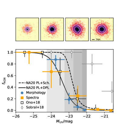
Figure 7: The AGN fraction as a function of absolute UV magnitude at $z=4$, derived from morphology/size criteria (blue circles) and from spectroscopy (orange squares). We compare to previous estimates of the AGN fraction at $z=4$ from Ono et al. (2018) and the $z=2$–$3$ results from Sobral et al. (2018) as the open black squares and grey diamonds respectively. The lines show the predicted $f_{\rm AGN}$ from the simultaneous fitting of the LBG and AGN LF presented in Adams et al. (2020). The dashed and solid lines show the results assuming a Schechter and DPL form for the LBG LF respectively. The four images in the upper row show the result of stacking our sample in the four grey highlighted bins in $M_{\rm UV}$ shown on the plot. The stamps are $1.5\,{\rm arcsec}$ on a side, with contours at intervals of $1.0\,{\rm mag}$ from the peak.

We present the derived $f_{\rm AGN}$ measurements in Fig. 7. Both the morphological and spectroscopic measurements show a sharp drop in the $f_{\rm AGN}$ between $-24\lesssim M_{\rm UV}\lesssim-22.5$, with around equal occurrence of AGN and LBGs at around $M_{\rm UV}\simeq-23.2$. This is also visually apparent in the stacked HST/ACS images (top of Fig. 7), where at $M_{\rm UV}\simeq-23$ the stack is clearly extended (although with less flux in the wings) while at $M_{\rm UV}\simeq-23.8$ the image is consistent with being a point-source. Comparing to previous estimates of the $f_{\rm AGN}$ at $z\simeq 4$ we find good agreement with the spectroscopy measurements of Ono et al. (2018), who used predominantly archival redshifts with spectroscopic flags to determine the AGN fraction. The advantage of our method of AGN classification from the full spectrum is that we are not sensitive to differences between AGN classifications between spectroscopic surveys. We find a brighter transition magnitude than that of Sobral et al. (2018), who found a drop in the fraction of AGN at $M_{\rm UV}=-21.5$ at $z\simeq 2$–$3$. This study was based on the follow-up of strong Lyman-$\alpha$ emitters rather than LBGs, and hence it could be expected that this pre-selection for strong line-emitters would preferentially detect AGN at fainter magnitudes. We note however, that in Sobral et al. (2018) the AGN fraction at $M_{\rm UV}>-22.5$ is determined from sources predominantly from a detection of the NV line with low S/N ($\lesssim 3.0$), their classification as AGN is somewhat uncertain.

At $-23<M_{\rm UV}<-22$ we see a slight difference in the derived AGN fraction from our morphological and spectroscopic measurements. From a morphology cut we measure $f_{\rm AGN}=0.06^{+0.03}_{-0.02}$ at $M_{\rm UV}=-22.5$ while with spectroscopic data we find $f_{\rm AGN}=0.25^{+0.17}_{-0.12}$. Although the errors are large, due predominantly to the small number statistics for the spectroscopic sub-sample, a difference between the $f_{\rm AGN}$ between a strict morphological selection and spectroscopic identification could be expected in this magnitude range. This is a consequence of the increasing importance of host galaxy light at fainter UV magnitudes, and we present a toy model that can explain these observations in Section 6. Alternatively the slight difference found could be due to bias in the spectroscopic measurement, as arguably the strong emission lines from AGN and the compactness of the emission could make them easier to identify in spectroscopic measurements. In the range $-23<M_{\rm UV}<-22$ we find no difference between the sizes of the spectroscopically confirmed sources and our full sample, suggesting that we are not biased to compact sources. In this magnitude range we find 10 sources with archival spectroscopy, four from the VANDELS survey and six from VVDS (of which eight with secure flags are shown in Fig. 5). While VVDS is a purely I-band magnitude limited survey, VANDELS selected against compact sources over 50 percent of the survey area that was covered by HST imaging (McLure et al., 2018), and hence VANDELS should be biased against AGN. If we measure the $f_{\rm AGN}$ in the VVDS and VANDELS survey separately, we find $f_{\rm AGN}=0.25^{+0.25}_{-0.15}$ for both surveys when secure flags are used, indicating that there is no clear bias within the limitations of small number statistics. Two of the VVDS spectra were not included in our initial AGN fraction calculation as they have poor quality flags. If we assume these objects are SF-dominated, under the assumption that AGN features are easier to identify, then we obtain a lower $f_{\rm AGN}=0.20^{+0.15}_{-0.10}$ in this magnitude range. This value is still higher than that derived from our morphology measurement, however larger spectroscopic samples are clearly required to determine if there is a real discrepancy between the $f_{\rm AGN}$ found from a strict morphological cut in contrast to a classification from spectroscopy.

In Fig. 7 we also present the predicted AGN fraction from the simultaneous fitting of the combined AGN and LBG LF presented in Adams et al. (2020). Adams et al. (2020) assumed either a Schechter function or DPL form for the LBG LF in addition to a single power-law (PL) to model the faint-end of the AGN. Without any further information about the nature of the sources, both models produced a good fit for the observed UV LF over $-26<M_{\rm UV}<-20$ (see left panel of Fig. 8). In comparison to our derived $f_{\rm AGN}$ we see that the Schechter function form of the LBG LF predicts a steeper decline in the fraction of AGN at fainter magnitudes than a DPL model, due to the exponential drop-off at the bright-end of this parameterisation. Note that the position of this drop depends on the position of the ‘knee’ in the LF, which is strongly constrained by the number density of sources $M_{\rm UV}>-21$. Both our measurements of the AGN fraction deviate from this steeper Schechter prediction at $M_{\rm UV}\sim-24$, as do the results of Ono et al. (2018), suggesting that a DPL is the more appropriate function to describe the LBG LF at $z\simeq 4$.

4.2 The Luminosity Function

In the previous section we compared the observed $f_{\rm AGN}$ to that expected from the fitting of the full AGN + LBG rest-frame UV LF. In this section we instead use the $f_{\rm AGN}$ derived in this study to separate the LF results of Adams et al. (2020) into AGN and SF-dominated subsamples. Because we could only classify a small fraction of the full sample using the morphology and spectroscopy data (e.g. because high-resolution imaging was only available in COSMOS, and the spectroscopy data only covers $\sim 1$ percent of the sample), we elected to apply the $f_{\rm AGN}$ to the data points from Adams et al. (2020) as opposed to recalculating the LF from a significantly smaller sample. We determined the separate LFs by using the AGN fractions derived from the morphology and spectroscopy results separately. To interpolate the $f_{\rm AGN}$ we fit a constrained model to our binned AGN fraction points shown in Fig. 7. The model consisted of two power-laws to approximate the overlap between the bright-end of the galaxy LF and the faint-end of the AGN LF without over-fitting the data. Due to the difference in the $f_{\rm AGN}$ derived from using the morphological and spectroscopic data, we find differences in the separate LFs for the AGN and SF dominated sources as shown in the two right-hand plots in Fig. 8.

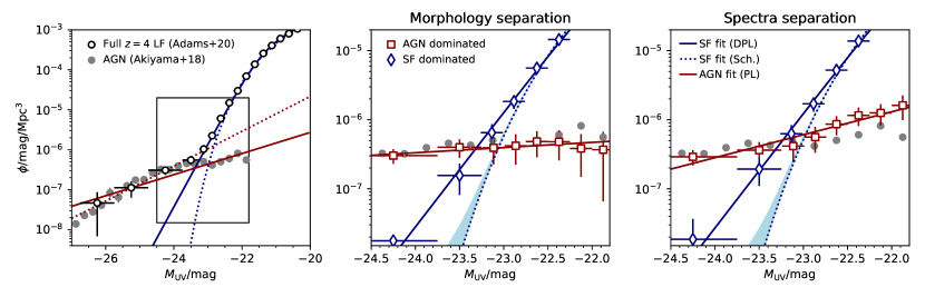
Figure 8: The rest-frame UV LF at $z\simeq 4$. The left-hand panel shows the full LF derived in Adams et al. (2020) as the open black circles. The solid (dotted) lines on this plot show the result of the simultaneous fitting presented in Adams et al. (2020) with a DPL (Schecher) assumed galaxy LF. The central and right-hand plots show a zoom-in of the transition region, where we have separated objects that have rest-frame UV light that is SF (blue diamonds) or AGN (red squares) dominated. In these plots we show the best-fit AGN power law as the red line. The best-fit Schechter or DPL function to the SF-dominated results are shown as the blue dotted and solid lines respectively. For the Schechter function the fit is constrained by points that are fainter than $M_{\rm UV}=-22$. The effect of the magnification bias on the Schechter function is shown as the blue shaded excess on this curve. In all three plots we show the AGN results from Akiyama et al. (2018) as the grey filled circles.

We present the results of fitting the separated AGN and SF-dominated LFs with different parameterisations in Fig. 8. The best-fit parameters are presented in Table 1 in comparison to the LF parameters derived from the simultaneous fit of Adams et al. (2020). The AGN fractions derived from these fits in comparison to the results of Adams et al. (2020) are presented in Appendix B. We fit our separated AGN-dominated UV LFs using a single power-law, as we do not extend faint-ward of the apparent LF knee at $M_{\rm UV}\sim-26$. For the SF LF we fit using both a Schechter function or a DPL. If we focus first on the SF-dominated results, we find that the separation of sources using a morphology or spectroscopy criterion makes only a marginal difference to the derived LF. This is evident in the fitting results presented in Table 1, where the values are well within the $1\sigma$ errors in the different scenarios. We also find good consistency with the Schechter and DPL parameters from Adams et al. (2020), which is to be expected as the LBG fit is predominantly constrained by the data-points at $M_{\rm UV}>-22$. We checked that the impact of strong gravitational lensing on a Schechter function fit could not reproduce the number of bright sources by applying the methodology of Mason et al. (2015); Barone-Nugent et al. (2015). The excess that results from the lensing is shown in Fig. 8 and is too small to account for the number density we find at $M_{\rm UV}<-23$.

In contrast to the SF-dominated LF, the faint-end of the AGN-dominated LF depends more significantly on the assumed $f_{\rm AGN}$. If we use a morphology criterion we find a shallow slope ($\alpha=-1.19\pm 0.05$) due to the rapid drop in point-source dominated sources faint-ward of $M_{\rm UV}\simeq-23$. In this case, we find close agreement with the results of Akiyama et al. (2018), who derived a faint-end slope of $\alpha=-1.30\pm 0.05$. This is to be expected given that Akiyama et al. (2018) identified AGN based on a compactness criterion in the ground-based HSC data. If instead we use our spectroscopic criterion in determining $f_{\rm AGN}$ we find a significantly steeper slope of the faint-end of the AGN LF of $\alpha=-1.85\pm 0.05$. In this case our data points start to diverge from the Akiyama et al. (2018) points, due to a higher proportion of AGN-dominated sources at faint magnitudes in this parameterisation (see Fig. 7). Adams et al. (2020) found $\alpha=-1.66^{+0.29}_{-0.58}$ in the fit of a DPL (LBG component) with a PL (AGN component). The large error on this value is a consequence of the degeneracy between the bright-end slope of the LBG LF and the AGN faint-end slope. Our measurement of the slope of the faint-end of the AGN LF is more constrained by the data-points at $M_{\rm UV}\gtrsim-24$, which allows us to find a best-fit that is shallower, but still consistent within $1.5\sigma$, from the Adams et al. (2020) result.

Table 1: The luminosity function parameterisations for the separated SF and AGN results shown in Fig. 8. The upper part of the table shows the results when separating according to a morphological criterion, while the lower part shows the results when AGN are identified according to their spectra. The first column indicates the sub-sample that was fit to (SF-dominated or AGN-dominated). For the SF case, we show the results for a Schechter function and DPL fit in the first and second row. The fit to the AGN case was performed with a single power law, with the normalisation calculated at a fixed $M_{\rm UV}$ highlighted with an asterick. The second and third column denote the characteristic absolute magnitude and normalisation. The fourth column show the faint-end slope for the SF and AGN fits, and the final column shows the bright-end slope for the DPL fit.

Type	$M^{*}$	$\phi^{*}$	$\alpha$	$\beta$
	$/{\rm mag}$	$/{\rm mag}/{\rm Mpc}^{3}$
SF	$-21.00(0.10)$	$1.36(0.24)\times 10^{-3}$	$-1.75(0.13)$	–
SF	$-21.53(0.06)$	$0.36(0.05)\times 10^{-3}$	$-2.07(0.07)$	$-5.15(0.10)$
AGN	-25.70*	$2.48(0.31)\times 10^{-7}$	$-1.19(0.05)$	–
SF	$-20.97(0.09)$	$1.44(0.25)\times 10^{-3}$	$-1.72(0.13)$	–
SF	$-21.50(0.05)$	$0.37(0.04)\times 10^{-3}$	$-2.05(0.06)$	$-5.15(0.09)$
AGN	-25.70*	$0.77(0.21)\times 10^{-7}$	$-1.83(0.11)$	–
Adams et al. (2020)
Sch.	$-20.89^{+0.12}_{-0.10}$	$1.62^{+0.33}_{-0.27}\times 10^{-3}$	$-1.66^{+0.13}_{-0.08}$	–
+PL	-25.70*	$0.71^{+0.44}_{-0.39}\times 10^{-7}$	$-2.09^{+0.32}_{-0.38}$	–
DPL	$-21.37^{+0.08}_{-0.11}$	$0.50^{+0.10}_{-0.06}\times 10^{-3}$	$-1.92^{+0.07}_{-0.04}$	$-4.92^{+0.29}_{-0.25}$
+PL	-25.70*	$0.85^{+0.81}_{-0.34}\times 10^{-7}$	$-1.66^{+0.29}_{-0.58}$	–

5 Discussion

In this work we have investigated the transition in the properties of $z\simeq 4$ sources at $M_{\rm UV}\simeq-23$, where the number densities of faint-AGN and bright-galaxies converge. From our imaging data we observe a change in the source morphology, through a sharp drop in the average size of sources in the size-luminosity relation that is also seen in the individual source morphology. We also see a change in the features present in the available rest-frame UV spectra for the sample. The absolute UV magnitude at which this transition occurs corresponds to the point of rapid decline in the bright-end of the galaxy LF. Furthermore, the form of the increase in the AGN fraction to brighter magnitudes depends on the shape of the galaxy LF bright-ward of the knee in the function ($M_{\rm UV}\simeq-21$; see Table 1). There has been an ongoing discussion on the shape of the rest-frame UV at high-redshifts. While the UV LF at $z\gtrsim 4$ has typically been fitted by a Schechter function (e.g. McLure et al., 2013; Finkelstein et al., 2015; Bouwens et al., 2015), recent results have demonstrated an excess of highly luminous galaxies in relation to the Schechter function predictions (Bowler et al., 2014; Ono et al., 2018; Bowler et al., 2020). In our derived AGN fraction, and in the corresponding SF-dominated LFs, we have found evidence for a shallower decline in the number density of the brightest SF galaxies at $z\simeq 4$. Most strikingly, the discovery of an extremely bright source at $M_{\rm UV}=-23.6$ with no evidence for AGN spectral features (ID1448401 in Fig. 5) supports a $f_{\rm AGN}\simeq 0.8$ (range within the errors of $0.38$–$0.95$) at this magnitude, which leads to a number density of sources well in excess of the Schechter function prediction. This finding is potentially in conflict with studies that have found support for a Schechter function form at $z\simeq 3$–$4$ (van der Burg et al., 2010; Hathi et al., 2010; Bian et al., 2013; Parsa et al., 2016), however it is only recently that the datasets available at $z\simeq 4$ have had sufficient volume to adequately constrain the number density of the rarest galaxies/faint-AGN. If we fit our SF-dominated LF with a DPL, the results are in good agreement with the evolution in the DPL parameters derived in Bowler et al. (2015); Bowler et al. (2020), who found a steady steepening of the bright-end from $z\simeq 9$ to $z\simeq 5$ consistent with the increasing impact of dust. If this steepening is due to dust obscuration in the most highly star-forming galaxies, then the effects of this dust should be observable both in the colours of bright LBGs and directly via reprocessed emission in the far-infrared. Interestingly, the brightest spectroscopically confirmed LBG in our sample (ID1448401) shows a very blue rest-frame UV continuum (rest-frame UV slope $F_{\lambda}\propto\lambda^{\beta}$; $\beta\simeq-2$). From the observed colour-magnitude relation at this redshift, this source would be expected to show a redder slope with $\beta\simeq-1.4$ (Lee et al., 2011; Bouwens et al., 2014). Rogers et al. (2014) demonstrated that at $z\simeq 5$ there is an increased scatter in the rest-frame UV slopes of LBGs to brighter magnitudes, and thus it is plausible that this LBG is a rare example of a highly star-forming galaxy ($SFR\simeq 80\,{\rm M}_{\odot}/{\rm yr}$;  Madau et al., 1998) with little dust attenuation at this redshift. Thus while overall the increased production and attenuation of dust in the most highly SF galaxies from $z\simeq 9$–$4$ could cause a steepening of the bright-end slope of the rest-frame UV LF, this does not preclude the existence of galaxies with high-SFRs and a lack of dust obscuration within this epoch.

5.1 The faint-end of the AGN UV LF

There has been a renewed interest in recent years on the slope of the faint-end of the rest-frame UV LF of AGN. This was motivated by the claimed detection of high-redshift X-ray sources by Giallongo et al. (2015), who used their data to suggest that UV-faint AGN could contribute significantly to the process of reionization at $z>6$. Such an analysis relies on the integral of an extrapolated rest-frame UV LF to determine the total number of ionizing photons that can be produced by AGN at very high-redshifts. The subsequent studies of Boutsia et al. (2018) and Giallongo et al. (2019) have further claimed an excess in sources at the faint-end of the $z\simeq 4$. While several works have called these results into question (e.g. Parsa et al., 2018; McGreer et al., 2018; Cowie et al., 2020) at $z>4$, the determination of an accurate slope of the faint-end of the AGN LF remains of interest. Our observations demonstrate that the derived slope of the $z\simeq 4$ AGN LF depends strongly on the selection method. We can reproduce the flatter slope found in Akiyama et al. (2018) by using a criterion on morphology to separate AGN-dominated sources from the full $z\simeq 4$ LF. If instead we use a spectroscopic determination of $f_{\rm AGN}$ to estimate the AGN LF, we derive a steeper faint-end slope ($\alpha\sim-1.8$). The rest-frame UV spectroscopic features of AGN are strong and broad emission lines (e.g. Fig. 5), while LBGs are expected to show absorption features or potentially weak nebular emission lines (Stark et al., 2014; Shapley et al., 2003; Steidel et al., 2016). Thus we expect any classification of a source as an AGN based on the rest-frame UV spectrum to be sensitive to not only the brightest AGN-dominated objects, but also objects in which the light from SF is significant. Instead, AGN selections that include a point-like morphology selection will exclude objects where the host galaxy UV light causes the source to be rejected as too extended. Given the wide range in imaging depths and compactness criterion used in different AGN selections, it is challenging to understand the incompleteness of previous studies due to this effect. It is clear however, from our study and other works (e.g. Matsuoka et al., 2018b), that faint-ward of $M_{\rm UV}\simeq-24$ it is necessary to account for both AGN and SF-dominated sources.

5.2 Evolution of the AGN to SF transition into the EoR

Both the AGN and LBG rest-frame UV LFs are known to evolve rapidly at $z\gtrsim 4$. In Bowler et al. (2020) we found evidence for a flattening of the bright-end slope with increasing redshift in the range $z=5$–$10$, with a corresponding evolution in $M^{*}$ according to $\Delta M^{*}/\Delta z\simeq-0.5$. This was interpreted as a result of decreased dust obscuration and mass quenching within the Epoch of Reionization (EoR). Such a change in shape would be imprinted onto the measured AGN fraction at these redshifts, with a predicted fainter transition magnitude and extended tail of highly luminous SF galaxies. This prediction is consistent with the tentative detection of weak AGN features in the rest-frame UV spectra of moderately bright LBGs at $z\gtrsim 6$ (Laporte et al., 2017; Tilvi et al., 2016), as we predict a higher $f_{\rm AGN}$ to fainter magnitudes within this epoch. These detections however, are at odds with the expected number density of faint AGNs at $z\simeq 6$, which have been shown to undergo an accelerated decline at $z>5$ (McGreer et al., 2013; Jiang et al., 2016). From the extrapolated number densities of high-redshift AGN, we do not expect that current LBG samples at $z\geq 7$ will contain any AGN-dominated sources, as AGN are only expected to be more numerous than LBGs at $M_{\rm UV}\leq-24$ (see discussion in Bowler et al., 2014). This is consistent with the lack of point-sources found at $z\simeq 6$–$7$, where it has been possible to gain high-resolution imaging of the brightest sources with HST (Jiang et al., 2013; Bowler et al., 2017). These somewhat conflicting results could be a result of weaker AGN residing within high-redshift LBGs, or misclassification of emission lines as AGN signatures. Taking the results of this study coupled with what is known about the evolving UV LFs to higher redshifts, we predict that AGN ‘contamination’ of rest-frame UV selection samples faint-ward of $M_{\rm UV}\simeq-23$ will be minimal at $z\geq 7$.

6 A simple model of the AGN UV LF

We created a toy model of the predicted rest-frame UV LF of AGN to aid in the interpretation of our observations. The model takes the observed UV LF of LBGs and uses this, via simple empirical relations, to estimate the luminosity and number density of UV-bright AGN at the same epoch.

6.1 Method

For each galaxy of a given absolute UV magnitude, we first estimate the stellar mass according to the relation found by Duncan et al. (2014):

$${\rm log}_{10}(M_{\star})=(9.02\pm 0.02)\,(M_{\rm UV}+19.5)-(0.45\pm 0.02).$$ (1)

The slope and normalisation of this relation is consistent between different studies (e.g. Salmon et al., 2015; Song et al., 2016; see figure 5 of Tacchella et al., 2018). This relation has been derived in the past to determine the stellar mass functions at high-redshift from the rest-frame UV LF, where the effect of scatter is essential in order to reproduce the observed mass and LFs (Stark et al., 2013; Duncan et al., 2014). We therefore include a scatter of $0.4\,{\rm dex}$ in the relationship above, which is consistent with that required in Duncan et al. (2014) and is at the upper end of the measured intrinsic scatter in the $SFR$–$M_{\star}$ relation (Curtis-Lake et al., 2020; Salmon et al., 2015). From the stellar mass we then estimate the black hole mass using the $m_{\rm BH}-M_{\star}$ relation of the form:

$${\rm log}_{10}(m_{\rm BH})=G_{\rm BH}\,[{\rm log}_{10}(M_{\star})+11.0]+I_{\rm BH}$$ (2)

Here $G_{\rm BH}=d{\rm log}_{10}(m_{\rm BH})/dM_{\star}$ gives the gradient of the relation and $I_{\rm BH}$ the intercept (defined at a mass of ${\rm log}_{10}(M_{\star}/{\rm M}_{\odot})=11.0$). The form or even existence of such a relationship at high-redshift is uncertain. We therefore consider two plausible scenarios based on previous results from both luminous quasars at high-redshift and low-redshift galaxies. The simplest scenario is one in which the black-hole mass is a constant fraction of the stellar mass at a given redshift. In this case (denoted model A hereafter) we set $G_{\rm BH}=1.0$ and $I_{\rm BH}=9.0+{\rm log}_{10}(1+z)$ to give $m_{\rm BH}/M_{\star}=0.05$ at $z=4$, as found in observations of high-redshift quasars (e.g. Venemans et al., 2017; Targett et al., 2012). The $1+z$ term follows observations and theoretical arguments for an increased $m_{\rm BH}$ to bulge-mass ratio at high-redshifts (e.g. Venemans et al., 2015; Croton, 2006; Wyithe & Loeb, 2003). Such high ratios of $m_{\rm BH}/M_{\star}$ may not be representative of the AGN population at this redshift (e.g due to selection effects), hence we treat this scenario as an extreme case. An alternative scenario is one in which black holes in more massive galaxies are over-developed, whereas those in less massive sources are a smaller fraction of the stellar mass. Such a scenario has been measured at low-redshift by Reines & Volonteri (2015). In this case (denoted as model B hereafter) we set $G_{\rm BH}=1.4$ and $I_{\rm BH}=8.95+{\rm log}_{10}(1+z)$. Scatter is also significant in the $m_{\rm BH}$-$M_{\star}$ relation (e.g.see Hirschmann et al., 2010; Volonteri & Reines, 2016), and we therefore include an intrinsic scatter of $0.3\,{\rm dex}$. The result of these steps is a relationship between the $M_{\rm UV}$ of a LBG and the estimated $m_{\rm BH}$. The $m_{\rm BH}$ can then be converted into an estimated bolometric luminosity using an assumption on the Eddington ratio. We assume a log-normal distribution of mean $\lambda=0.6$ and $\sigma=0.3\,{\rm dex}$ as found by Willott et al., 2010b (see also Kelly & Shen, 2013). Finally we convert the bolometric luminosity into a UV luminosity by assuming a bolometric correction (taken to be $4.4$; Runnoe et al., 2012; Mortlock et al., 2011). From a single $M_{\rm UV}$ from SF we thus obtain a spread in the predicted total absolute UV magnitude due to the addition of an unobscured black hole ($M_{\rm UV,BH}$).

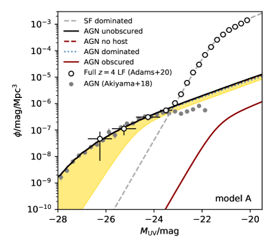
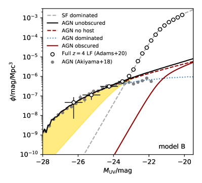
Figure 9: The predicted rest-frame UV LF of AGN as derived from our simple models. The upper plot shows the results for a model where $m_{\rm BH}/M_{\star}=0.05$ (model A), and the lower plot shows the results where $m_{\rm BH}\propto M_{\star}^{1.4}$ (model B). The grey dashed line shows the DPL fit to the rest-frame UV LF for star-forming galaxies from Adams et al. (2020). The result of applying empirical scaling relations, with scatter, to this galaxy LF results in the AGN prediction shown as the black line. The effect of scatter is highlighted as the gold shaded region, such that the lower edge of this shading would be the prediction with no scatter. The red solid line shows the predicted obscured Type II AGN LF, and the blue dotted line shows the expected LF for sources in which $L_{\rm BH}/L_{\rm SF}>12.5$. The red dashed line shows the predicted AGN LF without the UV emission from the host galaxy. The open circles show the measurements from Adams et al. (2020) and the grey filled circles show the results from Akiyama et al. (2018), who imposed a criterion on the source morphology.

Following these steps resulted in a simulated AGN LF with a relative flat shape at the bright-end. This is in contrast with the knee in the function around $M_{\star}\sim-26$ found in observations. This effect arises in our model from the creation of infeasibly massive black holes and galaxies, due to the application of scatter in the relations between $M_{\rm UV}$, $M_{\star}$ and $m_{\rm BH}$. While the form of the bright-end of the AGN LF does not impact the results of this work, we nevertheless impose a crude cut in the stellar and black-hole masses to remove these unrealistic sources. We take a limiting stellar mass of ${\rm log}_{10}(M_{\star})=10.8$ from the characteristic mass of high-redshift galaxies (e.g. Ilbert et al., 2013; McLeod et al., 2020), and impose an upper limit on the black-hole mass of ${\rm log}_{10}(m_{\rm BH})=9.5$ to approximate the drop in the (uncertain) black-hole mass functions at $z\simeq 4$ (e.g. Shankar et al., 2009; Kelly & Merloni, 2012). If a model galaxy/black hole exceeds these mass limits due to scatter, we allocate a lower mass at random according to the relations described above. The result of this simple process is a knee in the AGN LF in good agreement with the observations. We calculate the results of this analysis for both the Schechter and DPL form presented in Adams et al. (2020), where they fitted to only points at $M_{\rm UV}>-22.0$ to ensure that the results were not influenced by AGN-dominated sources. The resulting AGN LF depends only weakly on the assumed shape of the LBG LF because the majority of the simulated AGN are hosted in galaxies with $M_{UV}>-22.0$ where there is good agreement between the Schechter and DPL fits. In contrast, the ratio of AGN to SF-dominated sources at $M_{\rm UV}\sim-23$ does rely on the LBG LF shape, as it depends on how steeply the LBG LF drops-off at the bright-end (see Section 5).

To obtain a predicted AGN LF that matches the number density of quasars known at $z\simeq 4$ we include two factors to modulate the number of LBGs that host an AGN. The first is the obscured fraction, which describes how many ‘on’ AGN are not bright in the rest-frame UV continuum (e.g. are obscured Type II AGN). We fixed $f_{\rm obsc.}=0.6$ (Ueda et al., 2014; Vito et al., 2018). The second modulating factor is the fraction of galaxies that host an active black hole, which is a proxy for the duty cycle of AGN activity. The $f_{\rm active}$ was determined in our model as the factor required to bring the predicted AGN LF in agreement with the observed AGN LF in the range $-27<M_{\rm UV}<-24$. We find $f_{\rm active}=0.0007$ for model A and $f_{\rm active}=0.003$ for model B. Note that $f_{\rm active}$ is not directly comparable to the duty cycle of AGN activity, as it is the fraction of AGN that appear bright in the rest-frame UV rather than the fraction of active black holes.

6.2 Results

We present the results of this analysis in comparison with the observed LBG and AGN rest-frame UV LF in Fig. 9. Despite the simplicity of the model, it does a reasonable job at reproducing the shape of the observed $z\simeq 4$ AGN LF at luminosities bright-ward of $M_{\rm UV}\simeq-23.5$. A striking feature of the predicted LFs shown in Fig. 9 is the dominant role of scatter which is well known to be important from observations of the brightest quasars (e.g. Venemans et al., 2017; Willott et al., 2013; Targett et al., 2012). Furthermore, both models predict a similarly steep faint-end slope consistent with that found by other empirical predictions (e.g. Veale et al., 2014; Ren et al., 2020; Delvecchio et al., 2020). For sources around $M_{\rm UV}\simeq-23$, our two models give different predictions for the importance of scatter in the observed galaxies. This has consequences for the expected morphology and spectroscopic properties of sources around this magnitude. The AGN LFs from our toy model do not show the flattening observed in the results of Akiyama et al. (2018) faint-ward of $M_{\rm UV}\simeq-24$. Akiyama et al. (2018) used a moment based measure to select compact sources in ground-based HSC data, while our model does not make any assumption about the size or morphology of each model galaxy/AGN. If we impose the condition that the AGN luminosity must be a certain multiple of the stellar light (e.g. $L_{\rm BH}/L_{\rm SF}\gtrsim 10$) then we are able to reproduce the flattening found in the data, but only in the case where the black-hole mass is an increasing fraction of the stellar mass (model B). The magnitude of the cut is motivated by previous studies comparing the host galaxy and AGN emission in the rest-frame UV and optical for sources selected as quasars (typically $\Delta M=2$–$3\,{\rm mag}$;  Jahnke et al., 2004; Schramm et al., 2008; Goto et al., 2009; Mechtley et al., 2016; Lawther et al., 2018) When fitting the Akiyama et al. (2018) points with the ratio as a free parameter, we found a best-fit ratio of $L_{\rm BH}/L_{\rm SF}=12.5\pm 0.5$ for model B. The drop in the AGN LF in this case is due to the host galaxy rest-frame UV light becoming significant at $M_{\rm UV}>-23$. Such a cut is incomplete to fainter AGN (relative to their host galaxy UV emission) and therefore results in an artificial flattening in the observed AGN LF as shown in Fig. 9. If instead black holes populate host galaxies as in our model A, where the effect of scatter in shaping the observed AGN LF at fainter magnitudes is dominant, then such a flattening is not predicted with this relative luminosity cut. The effect can also be seen in Fig. 10 where we compare the observed $f_{\rm AGN}$ to that predicted from our model. These results demonstrate that the morphological and spectroscopic properties of sources around $M_{\rm UV}\simeq-23$ gives important information about how active black holes are distributed within host galaxies. If the rest-frame UV is always dominated by light from the AGN, then selections based on a point-sources condition will be complete (model A). Such a selection will not be feasible to fainter magnitudes however, due to LBGs themselves becoming more compact. If instead the host galaxy light can become important at fainter magnitudes, as in our model B, then we see a distinct incompleteness in point-source selections for AGN at $M_{\rm UV}>-23$. In this case it becomes essential to define the relative ‘AGN-strength’ that is being included with a given selection methodology, to fully understand what population is being measured.

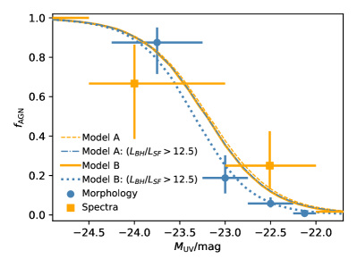
Figure 10: The predicted AGN fraction as a function of absolute UV magnitude at $z=4$ from our toy model. The models are compared to the derived fraction from our morphology (blue circles) and spectroscopy (orange squares) data. The yellow dashed (solid) lines show the predicted $f_{\rm AGN}$ from model A (B) with all AGN included. The blue dot-dashed (dotted) line corresponds to the $f_{\rm AGN}$ if a luminosity cut of $L_{\rm BH}/L_{\rm SF}$ is imposed to model A (B), to identify AGN-dominated sources. We see that with this cut model B is able to reproduce our observed morphology-based AGN fraction.

6.3 Obscured Type-II AGN

So far in this work we have considered only unobscured Type I AGN, which we expect to contribute significantly to the rest-frame UV continuum luminosity of the source. In the orientation-based unified model of AGN we also expect obscured Type II-like AGN, where the presence of an AGN is only observable in the UV via narrow emission lines. In our model of the AGN LF as derived from the LBG LF, we can predict the number density of these obscured sources. Interestingly, our preferred model (model B), which can better explain our observations of the $f_{\rm AGN}$ and the observed flattening of the faint-end slope found by Akiyama et al. (2018), also predicts an increased contribution of obscured AGN at $M_{\rm UV}>-22$. This is a natural consequence of our assumed active and obscured fractions of galaxies in the model. In model B we expect to see an increased contribution from obscured AGN at fainter magnitudes, with the number densities of ‘obscured’ and ‘unobscured’ sources becoming comparable (within a factor of $<5$) at $M_{\rm UV}\gtrsim-21$. While there are many assumptions and uncertainties in this prediction, we note that faint-ward of $M_{\rm UV}=-22$ we detect one source with clear AGN signatures in the compilation of spectra for our sample. This source, ID520330, appears to be an obscured Type II source (Fig. 6) at $M_{\rm UV}=-21$. From this one object we estimate the number density of obscured AGN at this magnitude is around $\phi=7\pm 7\times 10^{-6}\,/{\rm mag}/{\rm Mpc}^{3}$, which despite the huge uncertainties is within a factor of ten from our model prediction (model B: Fig. 9). These arguments demonstrate that there is still considerable uncertainty in the faint-end of the $z\simeq 4$ AGN UV LF depending on how AGN are defined and on the selection procedure. Given the large samples of $z\simeq 4$ sources available to-date from deep optical/NIR surveys (e.g. Adams et al., 2020; Ono et al., 2018; Bouwens et al., 2015), the next steps to overcome this challenge do not require substantial increases in sample size. Rather, in this work we have demonstrated that with a combination of magnitude limited spectroscopic follow-up, coupled with high-resolution imaging, it will be possible to probe the connection between faint-AGN and their galaxy hosts.

7 Conclusions

We present the size, morphology and spectroscopic properties of a sample of $3.5<z<4.5$ galaxies and AGN selected based on a photometric redshift fitting analysis in Adams et al. (2020). The broad magnitude range probed by the parent sample ($-26\lesssim M_{\rm UV}\lesssim-20$) allows us to uniquely probe the transition between SF- and AGN-dominated sources. We use both ground-based and HST imaging data to identify the changes in morphology and size, and archival spectra to detect signatures of AGN in the rest-frame UV spectrum. The key conclusions of this study are as follows.

• We find the expected galaxy size-luminosity relation up to an absolute UV magnitude of $M_{\rm UV}=-22.5$, beyond which we observe a steep downturn due to the increasing presence of objects with a point-source morphology. The effect is seen in both the high-resolution HST $I_{814}$ imaging and the ground-based data. We find that brightest galaxies in the sample have a highly irregular structure as expected from previous works.

• The existence of archival spectra for a sub-set of our sample allows us to identify SF and AGN dominated sources from the rest-frame UV spectral signatures. At the bright-end of our sample we see clear AGN signatures in the available spectra, while deep spectroscopy from targeted high-redshift surveys show the expected features of LBGs. We identify a very bright source $M_{\rm UV}=-23.6$ ($SFR\simeq 80\,{\rm M}_{\odot}/{\rm yr}$) that shows no evidence for an AGN contribution to the rest-frame UV light.

• We combine the morphology/size and spectroscopy information to estimate the AGN fraction as a function of $M_{\rm UV}$. We find a steep transition at $M_{\rm UV}\simeq-23.2$ where the number of bright galaxies drops while AGN-dominated sources become ubiquitous. We find a slight tension in the $f_{\rm AGN}$ derived independently from our morphology and spectroscopy data at $M_{\rm UV}\simeq-22.5$, with the spectroscopy results finding a higher fraction by a factor of $\sim 5$.

• We use this AGN fraction to estimate the separated AGN and SF-dominated rest-frame UV LFs at $z\simeq 4$. We find the bright-end of the SF-dominated LF to be described by a DPL with a bright-end slope of $\beta=-5.15\pm 0.10$. Our LBG UV LF is consistent with that expected from the observed steepening in $\beta$ from $z\simeq 9$–$5$ found by Bowler et al. (2020), which can be explained by an increased effect of dust attenuation in the most highly star-forming galaxies.

• We find that the slope of the faint-end of the AGN LF depends on how we determine the AGN fraction. If we impose a point-source morphology criterion, as in several recent studies of faint AGN, then we find a shallow slope with $\alpha=-1.19\pm 0.05$. Conversely, if we derive the AGN number density using the spectroscopic results we find a steeper slope of $\alpha=-1.83\pm 0.11$.

• A simple model of the AGN LF, derived using empirical relations applied to the LBG UV LF at $z=4$, can provide a good description of the transition from AGN to SF-dominated sources. By applying a criterion on the relative emission from the AGN and host galaxy ($L_{\rm BH}/L_{\rm SF}>15$), we are able to reproduce the observed flattening of the $z=4$ AGN LF at $M_{\rm UV}<-22$ found by Akiyama et al. (2018). This flattening is only predicted in the case that the light from SF becomes significant in comparison to the AGN in less massive galaxies.

Our results demonstrate that while the increasingly large samples of $z\simeq 4$ sources have resulted in low statistical errors on the rest-frame UV LF of AGN, there remain considerable systemic uncertainties on the faint-end of this function. In particular, the commonly imposed point-source criterion in the selection of AGN samples at these redshifts can result in incomplete samples of active sources at $M_{\rm UV}>-24$ due to the impact of the host galaxy. The degree of this incompleteness depends on how active black holes populate the underlying galaxy distribution and how these active sources appear in the rest-frame UV light accessible in optical datasets. Upcoming wide-area high-resolution imaging (e.g. from Euclid; Laureijs et al., 2012) with extensive spectroscopic follow-up (e.g. from degree-scale multi-object spectrographs like the William Herschel Telescope Enhanced Area Velocity Explorer; Dalton et al., 2012 and the Multi-Object Optical and Near-infrared Spectrograph; Cirasuolo, 2014) will be a powerful combination to understand further the co-evolution of galaxies and AGN at high redshifts.

Data Availability

The datasets used in this work were derived from sources in the public domain. Links to the online repositories and references to the survey data we utilized are listed in Section 2.

Appendix A Spectroscopically confirmed sources

In Table 2 we present the brightest sources in our parent sample that have been spectroscopically confirmed. In addition to the published spectroscopic redshift, for some of these sources we were able to obtain reduced spectra which we present in Fig. 5. As discussed further in Adams et al. (2020) we overlap with the majority of the Boutsia et al. (2018) sample. As part of our analysis we identified a discrepancy between the absolute magnitudes presented by Boutsia et al. (2018), which can be up to $1\,{\rm mag}$ fainter than the $M_{\rm UV}$ we calculated from our best-fitting SED model. In Boutsia et al. (2018) the $M_{\rm UV}$ is estimated by applying a $K$-correction to the $r-$band data, which typically hosts the Lyman-break from $z=3.9$–$4.7$. Our analysis demonstrates that this method can underestimate the $M_{\rm UV}$. In addition to this discrepancy, we find we cannot reproduce the higher number density of AGN derived by Boutsia et al. (2018) ($\phi=1.6\times 10^{-6}$ at $M_{\rm UV}=-23.5$). This is puzzling given that the majority of the Boutsia et al. (2018) sources are reselected in this work.

Table 2: The spectroscopically confirmed high-redshift sources from the full $z\simeq 4$ sample. We present the objects with $M_{\rm UV}<-22.0$, with the COSMOS and XMM-LSS sources in the upper and lower part of the table respectively. The first column is the source ID number followed by the R.A. and Declination. In column 3 we present the total HSC $I$-band apparent magnitude followed by the best-fitting photometric redshift with a Galaxy and QSO template in columns 4 and 5. In brackets after the photometric redshift is the $\chi^{2}$ of the fit. The final two columns denote the absolute UV magnitude followed by a note indicating the origin of the spectroscopic measurement. KB18 corresponds to Boutsia et al. (2018), zCOS to zCOSMOS, PR to Primus, VAN to VANDELS. We denote with an asterick the objects for which we were able to obtain the rest-frame UV spectrum, presented in Section 3.3.

ID	R.A.	Dec.	$I_{\rm HSC}$	$z_{\rm gal}$	$z_{\rm qso}$	$z_{\rm spec}$	$M_{\rm UV}$	Notes
188657	9:57:52.16	+1:51:20.08	21.20	0.27 (39.0)	3.92 (20.1)	4.174	-24.90	KB18(658294),zCOS*
203718	10:01:56.55	+1:52:18.80	21.88	4.19 (70.3)	4.28 (50.3)	4.447	-24.18	zCOS,PR*
657658	10:02:48.91	+2:22:11.88	21.69	3.75 (96.0)	3.52 (151.7)	3.748	-24.12	KB18(1163086),zCOS,PR*
702265	10:00:24.23	+2:25:09.86	22.55	4.28 (123.4)	4.36 (98.0)	4.596	-23.94	PR
153468	9:58:08.09	+1:48:33.10	22.40	3.92 (19.1)	3.88 (25.4)	3.986	-23.75	KB18(664641)
113309	10:00:25.77	+1:45:33.11	22.40	3.79 (126.7)	4.16 (87.0)	4.140	-23.72	KB18(330806)
677759	10:02:33.23	+2:23:28.74	22.45	3.50 (123.0)	3.72 (58.1)	3.650	-23.43	KB18(1159815)
724788	9:59:06.46	+2:26:39.39	22.35	3.73 (122.8)	3.92 (81.7)	4.170	-23.42	KB18(1273346),PR
523406	9:59:31.01	+2:13:32.88	22.46	3.48 (70.0)	3.60 (52.7)	3.650	-23.37	KB18(1054048)
908052	9:59:22.37	+2:39:32.63	23.49	3.72 (76.3)	4.08 (32.9)	3.748	-22.99	KB18(1730531)
840823	10:00:54.52	+2:34:34.90	23.75	4.43 (15.1)	4.56 (36.7)	4.539	-22.57	DEIMOS(842313)
112866	10:01:26.67	+1:45:26.16	23.87	4.44 (9.2)	4.60 (11.6)	5.137	-22.49	DEIMOS(308643)
654636	10:01:31.60	+2:21:57.73	24.01	4.48 (8.6)	4.52 (25.1)	4.511	-22.34	VUDS(5101210235)
606304	10:01:12.50	+2:18:52.58	24.09	4.46 (60.9)	4.44 (32.0)	5.691	-22.27	VUDS(5101218326)
697618	10:01:19.91	+2:24:47.47	24.21	4.46 (2.3)	4.56 (8.4)	4.419	-22.14	DEIMOS(733857)
278034	2:18:44.46	-4:48:24.59	19.74	4.13 (144.0)	4.44 (98.3)	4.574	-26.48	SDSS*
1364622	2:27:54.62	-4:45:35.37	20.31	3.60 (48.6)	3.72 (97.3)	3.741	-25.64	SDSS*
919928	2:24:13.41	-5:27:24.73	20.31	3.56 (44.2)	3.80 (24.2)	3.779	-25.55	SDSS*
1448906	2:25:27.23	-4:26:31.21	21.32	3.54 (66.1)	3.68 (29.3)	3.835	-24.57	PR, VVDS*
45737	2:18:05.65	-5:26:35.58	21.75	3.77 (45.5)	3.64 (102.1)	4.077	-24.21	PR
456332	2:17:14.17	-4:20:00.54	22.30	0.47 (65.4)	4.36 (52.2)	4.317	-24.12	PR
307263	2:18:31.37	-4:43:54.39	21.88	3.42 (32.0)	3.64 (13.9)	3.683	-24.03	PR
1448401	2:27:54.45	-4:26:37.97	22.29	3.63 (24.3)	3.64 (66.4)	3.835	-23.62	VVDS*
173860	2:17:34.38	-5:05:14.55	23.25	0.35 (63.9)	3.88 (28.2)	3.983	-22.72	VAN(199159)*
75407	2:17:53.11	-5:21:24.40	23.67	0.35 (14.0)	4.20 (10.0)	3.802	-22.64	VAN(141491)*
1499379	2:25:33.71	-4:15:41.51	23.68	0.42 (21.7)	4.28 (16.5)	3.699	-22.62	VVDS*
90440	2:18:05.17	-5:18:55.74	23.67	0.41 (15.5)	4.16 (9.6)	3.921	-22.58	VAN(150302)*
1463494	2:27:53.87	-4:23:20.34	23.37	3.36 (69.4)	3.56 (54.2)	3.626	-22.42	VVDS*
1485639	2:26:59.61	-4:18:32.88	23.67	3.82 (10.1)	4.08 (15.8)	3.872	-22.36	VVDS*
140721	2:17:33.77	-5:10:24.57	23.76	3.98 (13.4)	4.20 (22.3)	4.129	-22.33	VAN(018574)*
1522259	2:25:33.61	-4:10:57.99	23.79	4.12 (20.6)	4.28 (15.9)	4.116	-22.32	VVDS*

Appendix B AGN fraction from our fitting

In Fig. 11 we show the resulting AGN fractions derived from our fitting procedure to the separated AGN and SF UV LFs. We compare these to the results from Adams et al. (2020) who did not separate the two populations. In comparison to Adams et al. (2020) we find that the DPL and Schechter parameterisations of the SF-dominated sources are consistent within $1\sigma$. The observed differences in the $f_{\rm AGN}$ are instead found to be due to more significant changes in the derived parameters for the power-law fit to the AGN-dominated sub-sample. When a Schechter function form is assumed for the SF-dominated sources, the fit to the AGN-dominated objects has a shallower slope than in Adams et al. (2020), leading to a brighter point of transition. Conversely, when a DPL function form is assumed for the SF-dominated sources, the power-law fit to the AGN-dominated objects shows a higher normalisation and hence the transition point (where $f_{\rm AGN}\simeq 0.5$) moves faint-wards.

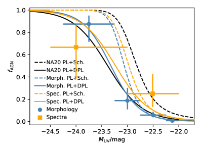
Figure 11: The results of our fitting to the separated AGN and SF-dominated sources. The solid (dashed) lines show the $f_{\rm AGN}$ derived when assuming a DPL (Schechter) function for the SF component. In both cases a power-law is assumed for the AGN component. The black lines show the results from a simultaneous fit of both types of sources by Adams et al. (2020). The blue (orange) lines show the results from this work, where we have separated SF and AGN-dominated sources according to the morphology (spectra). We reproduce our observed $f_{\rm AGN}$ points as in Fig. 7.

References

- Adams et al. (2020) Adams N. J., Bowler R. A. A., Jarvis M. J., Häußler B., McLure R. J., Bunker A., Dunlop J. S., Verma A., 2020, MNRAS, 494, 1771
- Akiyama et al. (2018) Akiyama M., et al., 2018, PASJ, 70, S34
- Alexandroff et al. (2013) Alexandroff R., et al., 2013, MNRAS, 435, 3306
- Bañados et al. (2016) Bañados E., et al., 2016, ApJSS, 227, 11
- Bañados et al. (2018) Bañados E., et al., 2018, Nat, 553, 473
- Barone-Nugent et al. (2015) Barone-Nugent R. L., Wyithe J. S. B., Trenti M., Treu T., Oesch P., Bouwens R., Illingworth G. D., Schmidt K. B., 2015, MNRAS, 450, 1224
- Bertin & Arnouts (1996) Bertin E., Arnouts S., 1996, A&AS, 117, 393
- Bian et al. (2013) Bian F., et al., 2013, ApJ, 774, 28
- Boutsia et al. (2018) Boutsia K., Grazian A., Giallongo E., Fiore F., Civano F., 2018, ApJ, 869, 20
- Bouwens et al. (2014) Bouwens R. J., et al., 2014, ApJ, 793, 115
- Bouwens et al. (2015) Bouwens R. J., et al., 2015, ApJ, 803, 34
- Bower et al. (2012) Bower R. G., Benson A. J., Crain R. A., 2012, MNRAS, 422, 2816
- Bowler et al. (2012) Bowler R. A. A., et al., 2012, MNRAS, 426, 2772
- Bowler et al. (2014) Bowler R. A. A., et al., 2014, MNRAS, 440, 2810
- Bowler et al. (2015) Bowler R. A. A., et al., 2015, MNRAS, 452, 1817
- Bowler et al. (2017) Bowler R., Dunlop J., McLure R., McLeod D., 2017, MNRAS, 466, 3612
- Bowler et al. (2020) Bowler R. A. A., Jarvis M. J., Dunlop J. S., McLure R. J., McLeod D. J., Adams N. J., Milvang-Jensen B., McCracken H. J., 2020, MNRAS, 2084, 2059
- Cirasuolo (2014) Cirasuolo M., 2014, SPIE, 9147, 91470N
- Clay et al. (2015) Clay S., Thomas P., Wilkins S., Henriques B., 2015, MNRAS, 415, 2692
- Coil et al. (2011) Coil A. L., et al., 2011, ApJ, 741, 8
- Cowie et al. (2020) Cowie L. L., Barger A. J., Bauer F. E., González-López J., 2020, ApJ, 891, 69
- Croton (2006) Croton D. J., 2006, MNRAS, 369, 1808
- Curtis-Lake et al. (2016) Curtis-Lake E., et al., 2016, MNRAS, 457, 440
- Curtis-Lake et al. (2020) Curtis-Lake E., Chevallard J., Charlot S., 2020, preprint (arXiv:2001.08560)
- Dalton et al. (2012) Dalton G., et al., 2012, SPIE, 8446, 84460P
- Dayal et al. (2014) Dayal P., Ferrara A., Dunlop J. S., Pacucci F., 2014, MNRAS, 445, 2545
- Delvecchio et al. (2020) Delvecchio I., et al., 2020, ApJ, 892, 17
- Duncan et al. (2014) Duncan K., et al., 2014, MNRAS, 444, 2960
- Eisenstein et al. (2011) Eisenstein D. J., et al., 2011, AJ, 142, 24
- Fan et al. (2003) Fan X., et al., 2003, AJ, 125, 1649
- Fèvre et al. (2019) Fèvre O. L., Béthermin M., Faisst A., Capak P., Cassata P., Silverman J. D., Schaerer D., Yan L., 2019, preprint(arXiv:1910.09517)
- Finkelstein et al. (2015) Finkelstein S. L., et al., 2015, ApJ, 810, 71
- Gavignaud et al. (2006) Gavignaud I., et al., 2006, A&A, 457, 79
- Giallongo et al. (2015) Giallongo E., et al., 2015, A&A, 578, A83
- Giallongo et al. (2019) Giallongo E., et al., 2019, ApJ, 884, 19
- Gonzalez-Perez et al. (2013) Gonzalez-Perez V., Lacey C. G., Baugh C. M., Frenk C. S., Wilkins S. M., 2013, MNRAS, 429, 1609
- Goto et al. (2009) Goto T., Utsumi Y., Furusawa H., Miyazaki S., Komiyama Y., 2009, MNRAS, 400, 843
- Grogin et al. (2011) Grogin N. A., et al., 2011, ApJS, 197, 35
- Hasinger et al. (2018) Hasinger G., et al., 2018, ApJ, 858, 77
- Hathi et al. (2010) Hathi N. P., et al., 2010, ApJ, 720, 1708
- Hirschmann et al. (2010) Hirschmann M., Khochfar S., Burkert A., Naab T., Genel S., Somerville R. S., 2010, MNRAS, 407, 1016
- Huang et al. (2013) Huang K.-H., Ferguson H. C., Ravindranath S., Su J., 2013, ApJ, 765, 68
- Ikeda et al. (2012) Ikeda H., et al., 2012, ApJ, 756, 160
- Ilbert et al. (2013) Ilbert O., et al., 2013, A&A, 556, A55
- Jahnke et al. (2004) Jahnke K., et al., 2004, ApJ, 614, 568
- Jiang et al. (2013) Jiang L., et al., 2013, ApJ, 773, 153
- Jiang et al. (2016) Jiang L., et al., 2016, ApJ, 833
- Kashikawa et al. (2015) Kashikawa N., et al., 2015, ApJ, 798, 28
- Kelly & Merloni (2012) Kelly B. C., Merloni A., 2012, Adv. in Ast., 2012
- Kelly & Shen (2013) Kelly B. C., Shen Y., 2013, ApJ, 764
- Kim et al. (2019) Kim Y., et al., 2019, ApJ, 870, 86
- Koekemoer et al. (2007) Koekemoer A. M., et al., 2007, ApJS, 172, 196
- Koekemoer et al. (2011) Koekemoer A. M., et al., 2011, ApJS, 197, 36
- Laporte et al. (2017) Laporte N., et al., 2017, ApJ, 837, L21
- Laureijs et al. (2012) Laureijs R., et al., 2012, in Clampin M. C., Fazio G. G., MacEwen H. A., Oschmann J. M., eds, Vol. 8442, Space Telescopes and Instrumentation 2012: Optical. p. 84420T, doi:10.1117/12.926496, http://adsabs.harvard.edu/abs/2012SPIE.8442E..0TL
- Law et al. (2012) Law D. R., Steidel C. C., Shapley A. E., Nagy S. R., Reddy N. A., Erb D. K., 2012, ApJ, 745, 85
- Lawther et al. (2018) Lawther D., Vestergaard M., Fan X., 2018, MNRAS, 475, 3213
- Le Fèvre et al. (2015) Le Fèvre O., et al., 2015, A&A, 576, A79
- Lee et al. (2011) Lee K.-s., et al., 2011, ApJ, 733, 99
- Lilly et al. (2007) Lilly S. J., et al., 2007, ApJS, 172, 70
- Lotz et al. (2006) Lotz J. M., Madau P., Giavalisco M., Primack J., Ferguson H. C., 2006, ApJ, 636, 592
- Madau et al. (1998) Madau P., Pozzetti L., Dickinson M., 1998, ApJ, 498, 106
- Mason et al. (2015) Mason C. A., et al., 2015, ApJ, 805, 79
- Massey et al. (2010) Massey R., Stoughton C., Leauthaud A., Rhodes J., Koekemoer A., Ellis R., Shaghoulian E., 2010, MNRAS, 401, 371
- Masters et al. (2012) Masters D., et al., 2012, ApJ, 752, L14
- Matsuoka et al. (2018a) Matsuoka Y., et al., 2018a, ApJS, 237, 5
- Matsuoka et al. (2018b) Matsuoka Y., et al., 2018b, ApJ, 869, 150
- Matute et al. (2013) Matute I., Masegosa J., Márquez I., Husillos C., Olmo A., Perea J., Povi M., 2013, A&A, 557, A78
- McGreer et al. (2013) McGreer I. D., et al., 2013, ApJ, 768, 105
- McGreer et al. (2018) McGreer I., Fan X., Jiang L., Cai Z., 2018, ApJ, 155, 131
- McLeod et al. (2020) McLeod D. J., McLure R. J., Dunlop J. S., Cullen F., Carnall A. C., Duncan K., 2020, 24, 1
- McLure et al. (2013) McLure R. J., et al., 2013, MNRAS, 432, 2696
- McLure et al. (2018) McLure R. J., et al., 2018, MNRAS, 479, 25
- Mechtley et al. (2016) Mechtley M., et al., 2016, ApJ, 830, 156
- Mortlock et al. (2011) Mortlock D. J., et al., 2011, Nat, 474, 616
- Oke (1974) Oke J. B., 1974, ApJS, 27, 21
- Oke & Gunn (1983) Oke J. B., Gunn J. E., 1983, ApJ, 266, 713
- Ono et al. (2018) Ono Y., et al., 2018, PASJ, 70, S10
- Parsa et al. (2016) Parsa S., Dunlop J. S., McLure R. J., Mortlock A., 2016, MNRAS, 456, 3194
- Parsa et al. (2018) Parsa S., Dunlop J. S., McLure R. J., 2018, MNRAS, 474, 2904
- Pentericci et al. (2018) Pentericci L., et al., 2018, A&A, 616, A174
- Reines & Volonteri (2015) Reines A. E., Volonteri M., 2015, ApJ, 813, 82
- Ren et al. (2020) Ren K., Trenti M., Di Matteo T., 2020, ApJ, 894, 124
- Richards et al. (2002) Richards G. T., et al., 2002, AJ, 123, 2945
- Richards et al. (2006) Richards G. T., et al., 2006, AJ, 131, 2766
- Rogers et al. (2014) Rogers A. B., et al., 2014, MNRAS, 440, 3714
- Runnoe et al. (2012) Runnoe J. C., Brotherton M. S., Shang Z., 2012, MNRAS, 422, 478
- Salmon et al. (2015) Salmon B., et al., 2015, ApJ, 799, 183
- Schramm et al. (2008) Schramm M., Wisotzki L., Jahnke K., 2008, A&A, 478, 311
- Scoville et al. (2007) Scoville N., et al., 2007, ApJS, 172, 1
- Shankar et al. (2009) Shankar F., Weinberg D. H., Miralda-Escudé J., 2009, ApJ, 690, 20
- Shapley et al. (2003) Shapley A. E., Steidel C. C., Pettini M., Adelberger K. L., 2003, ApJ, 588, 65
- Shen et al. (2003) Shen S., Mo H. J., White S. D. M., Blanton M. R., Kauffmann G., Voges W., Brinkmann J., Csabai I., 2003, MNRAS, 343, 978
- Shin et al. (2020) Shin S., et al., 2020, ApJ, 893, 45
- Sobral et al. (2018) Sobral D., et al., 2018, MNRAS, 482, 2422
- Song et al. (2016) Song M., et al., 2016, ApJ, 825, 5
- Stark et al. (2013) Stark D. P., Schenker M. A., Ellis R., Robertson B., McLure R., Dunlop J., 2013, ApJ, 763, 129
- Stark et al. (2014) Stark D. P., et al., 2014, MNRAS, 445, 3200
- Steidel et al. (2016) Steidel C. C., Strom A. L., Pettini M., Rudie G. C., Reddy N. A., Trainor R. F., 2016, ApJ, 826, 159
- Stevans et al. (2018) Stevans M. L., et al., 2018, ApJ, 863, 63
- Tacchella et al. (2018) Tacchella S., Bose S., Conroy C., Eisenstein D. J., Johnson B. D., 2018, ApJ, 868, 92
- Targett et al. (2012) Targett T. A., Dunlop J. S., Mclure R. J., 2012, MNRAS, 420, 3621
- Tilvi et al. (2016) Tilvi V., et al., 2016, ApJL, 827, L14
- Ueda et al. (2014) Ueda Y., Akiyama M., Hasinger G., Miyaji T., Watson M. G., 2014, ApJ, 786, 104
- Vanden Berk et al. (2001) Vanden Berk D. E., et al., 2001, AJ, 122, 549
- Veale et al. (2014) Veale M., White M., Conroy C., 2014, MNRAS, 445, 1144
- Venemans et al. (2015) Venemans B. P., Walter F., Zschaechner L., Decarli R., De Rosa G., Findlay J. R., McMahon R. G., Sutherland W. J., 2015, ApJ, 816, 37
- Venemans et al. (2017) Venemans B. P., et al., 2017, ApJ, 837, 146
- Vito et al. (2018) Vito F., et al., 2018, MNRAS, 473, 2378
- Volonteri & Reines (2016) Volonteri M., Reines A. E., 2016, ApJ, 820, L6
- Warren et al. (1994) Warren S. J., Hewett P. C., Osmer P. S., 1994, ApJ, 421, 412
- Willott et al. (2010a) Willott C. J., et al., 2010a, AJ, 139, 906
- Willott et al. (2010b) Willott C. J., et al., 2010b, AJ, 140, 546
- Willott et al. (2013) Willott C. J., Omont A., Bergeron J., 2013, ApJ, 770, 13
- Wyithe & Loeb (2003) Wyithe J. S. B., Loeb A., 2003, ApJ, 595, 614
- Yang et al. (2020) Yang J., et al., 2020, ApJ, 897, L14
- van der Burg et al. (2010) van der Burg R. F. J., Hildebrandt H., Erben T., 2010, A&A, 523, A74