123456

Basciftci and Van Hentenryck

Capturing Travel Mode Adoption in ODMTS

Capturing Travel Mode Adoption
in Designing On-demand Multimodal Transit Systems

Beste Basciftci Department of Business Analytics, University of Iowa, Iowa City, Iowa, 52242, USA, beste-basciftci@uiowa.edu Pascal Van Hentenryck Georgia Institute of Technology, Atlanta, Georgia 30332, USA, pvh@isye.gatech.edu

This paper studies how to integrate rider mode preferences into the design of On-Demand Multimodal Transit Systems (ODMTS). It is motivated by a common worry in transit agencies that the ODMTS may be poorly designed if the latent demand, i.e., new riders adopting the system, is not captured. The paper proposes a bilevel optimization model to address this challenge, in which the leader problem determines the ODMTS design, and the follower problems identify the most cost efficient and convenient route for riders under the chosen design. The leader model contains a choice model for every potential rider that determines whether the rider adopts the ODMTS given her proposed route. To solve the bilevel optimization model, the paper proposes an exact decomposition method that includes Benders optimal cuts and nogood cuts to ensure the consistency of the rider choices in the leader and follower problems. Moreover, to improve computational efficiency, the paper proposes upper and lower bounds on trip durations for the follower problems, valid inequalities that strenghten the nogood cuts, and approaches to reduce the problem size with problem-specific preprocessing techniques.

The proposed method is validated using an extensive computational study on a real data set from AAATA, the transit agency for the broader Ann Arbor and Ypsilanti region in Michigan. The study considers the impact of a number of factors, including the price of on-demand shuttles, the number of hubs, and access to transit systems criteria. The designed ODMTS feature high adoption rates and significantly shorter trip durations compared to the existing transit system and highlight the benefits in ensuring access for low-income riders. Finally, the computational study demonstrates the efficiency of the decomposition method for the case study and the benefits of computational enhancements that improve the baseline method by several orders of magnitude.

On-Demand Multimodal Transit Systems, Travel Mode Adoption, Benders Decomposition, Branch and cut

1 Introduction

This paper considers On-Demand Multimodal Transit Systems (ODMTS) (Mahéo et al. 2019, Van Hentenryck 2019), a new type of transit systems that combine on-demand shuttles with fixed routes served by buses or rail. ODMTS are organized around a number of hubs, on-demand shuttles serve local demand and act as feeders to and from the hubs, and fixed routes provide high-frequency service between hubs. By dispatching in real time on-demand shuttles to pick up riders at their origins and drop them off at their destinations, ODMTS are “door-to-door” and address the first/last mile problem that plagues most of the transit systems. Moreover, ODMTS address congestion and economy of scale by providing high-frequency services along high-density corridors. Figure 1 presents a sample ODMTS with buses between hubs along with the on-demand shuttles that can serve these hubs. They have been shown to bring substantial convenience and cost benefits in simulation and pilot studies in the city of Canberra, Australia (Mahéo et al. 2019), the transit system of the University of Michigan (Van Hentenryck 2019), the Ann-Arbor/Ypsilanti region in Michigan (Basciftci and Van Hentenryck 2020), and the city of Atlanta (Dalmeijer and Van Hentenryck 2020). ODMTS differ from micro-mobility in that they are designed and operated holistically. The ODMTS design thus becomes a variant of the hub-arc location problem (Campbell et al. 2005a, b): It is an optimization model that decides which bus/rail lines to open in order to maximize convenience and minimize costs (Mahéo et al. 2019). This optimization model uses, as input, the current demand, i.e., the set of origin-destination pairs in the existing transit system.

This paper is motivated by a significant worry of transit agencies: the need to capture latent demand in the design of ODMTS. This concern, which recognizes the complex interplay between transit agencies and riders (Cancela et al. 2015), was also raised by Campbell and Van Woensel (2019): they articulated the potential of (1) leveraging data analytics within the planning process and (2) proposing transit systems that encourage riders to switch transportation modes. As a consequence, rider preferences and the induced mode choices should be significant factors in the design of transit systems (Laporte et al. 2007). Yet, many transit agencies only consider existing riders when redesigning their network. But, as convenience improves, more riders may decide to switch modes and adopt the transit system instead of traveling with their personal vehicles. By ignoring this latent demand, the transit system may be designed suboptimally, resulting in higher costs or poor quality of service. Basciftci and Van Hentenryck (2020) illustrated these points by comparing the designs of ODMTS that differ by whether they capture latent demand. The results highlighted the significant cost increase when latent demand is not considered as the design under-invested in fixed routes and over-utilized on-demand shuttles. Note also that Agatz et al. (2020) highlighted the integration of stakeholder behavior in optimization models as a fundamental theme to address grand challenges in the next generation of transportation systems.

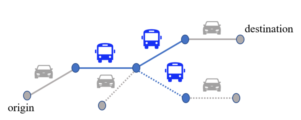
Figure 1: Illustration of the ODMTS with buses and on-demand shuttles. Hubs are denoted in blue color. Origin and destination stops are denoted in gray color. Solid lines represent the route of a rider from her origin to destination. Dashed lines represent potential bus legs between hubs or on-demand shuttles to/from the hubs.

Before presenting the design framework, it is useful to review how an ODMTS is used in practice. When a user requests a ride, she is presented with the route from origin to destination that jointly optimizes system cost and user convenience. The user then decides whether she takes the ride or uses a different transportation mode. It is thus important to realize that users do not choose their routes in the ODMTS: they are presented with routes in their mobile applications and decide whether to take them. If they could choose the routes, they would select a direct shuttle trip.

The key contribution of this paper is to propose a general framework to design an ODMTS based on both existing and latent demands. The framework assumes that the mode preference of a rider is expressed through a choice model which, given a route in the ODMTS, determines whether the rider adopts the ODMTS or continues to use her personal vehicle. The network design problem is then formulated as a bilevel optimization model which can be informally understood as follows. There is a subproblem associated with each trip by a rider: given a network design (i.e., a choice of bus routes to open), this subproblem chooses the route from the trip origin to the trip destination that optimizes a weighted combination of system cost and user convenience. The master problem chooses a network design, obtains the routes of each pair (trip,rider), and determines whether the riders take the proposed rides based in their choice models. The master problem optimizes an objective function that consists of several components: (1) the fixed cost of opening bus routes; (2) the cost and convenience of the trips accepted by the riders; and (3) the revenue of all adopted trips. The bilevel optimization model is solved using an exact decomposition method: it uses traditional Benders optimality cuts and nogood cuts, which are strengthened by valid inequalities exploiting the network structure. The approach is validated on a real case study.

The contributions of the paper can be summarized as follows:

1. The paper presents a bilevel optimization approach to the design of ODMTS under rider adoption constraints. The bilevel optimization problem consists of (i) a leader problem that determines the transit network design and takes into account rider preferences as well as revenues and costs from adopting riders; (ii) follower problems identify the most cost-efficient and convenient route for riders. The personalized choice models are integrated into the leader problem to represent the interplay between the transit agency and rider preferences. Since the model assumes a fixed cost for riding the transit system, the choice models capture the desired convenience of the trips.

2. The paper proposes an exact decomposition method for the bilevel optimization model. The method combines a Benders decomposition approach with combinatorial cuts that ensure the consistency between rider choices and the leader decisions. Furthermore, the paper presents valid inequalities that significantly strengthen these combinatorial cuts, as well as preprocessing steps that reduce the problem dimensionality. These enhancements produce orders of magnitude improvements in computation times.

3. The paper validates the approach using a comprehensive case study that considers the transit agency of the broad Ann Arbor/Ypsilanti region in Michigan. The case study demonstrates the benefits of the proposed approach from adoption, convenience, cost and access to transit systems perspectives. The results highlight that the ODMTS decreases trip durations by up to 53% compared to the existing system, induces high adoption rates for the latent demand, and operates well inside the budget of the transit agency.

The rest of the paper is organized as follows. Section 2 reviews the relevant literature. Section 3 presents the problem setting and the resulting bilevel ODMTS design problem with latent demand and rider choices. Section 4 proposes theoretical results on trip durations in ODMTS. Section 5 presents an exact decomposition algorithm and derives valid inequalities and problem-specific enhancements. Section 6 demonstrates the performance of the proposed approach in the case study. Section 7 concludes the paper with final remarks.

2 Related Literature

The design of transit networks organized around hubs is an emerging research area, with the goal of ensuring reliable service and economies of scale (Farahani et al. 2013a). Campbell et al. (2005a, b) introduce a variant of this problem, the hub-arc location problem, to select the set of arcs to open between hubs while optimizing the flow with minimum cost. Alumur et al. (2012) consider multimodal hub location and hub network design problem by taking into account both cost and convenience aspects in satisfying demand. Mahéo et al. (2019) examine this problem in the context of ODMTS, pioneering on-demand shuttles to serve all or parts of the trips, and allowing routes that do not necessarily involve arcs between hubs. The goal is to obtain a transit network design that minimizes the cost and duration of the overall trips. In these studies, user behaviour is not explicitly captured within the transit network design process; instead the objective function minimizes a weighted combination of the system cost and the travel times of the trips for existing riders of the transit system. Recently, Steiner and Irnich (2020) studied the design of an integrated public bus system with on-demand services. The paper points out the importance of optimizing over a mode-choice model for each origin-destination pair for determining rider preferences, and it mentions the resulting modeling and computational complexities. But the paper does not include mode-choice models: instead the formulation precomputes the induced demand based on the zones where on-demand service are provided.

Capturing information about rider routes into transit network design is a critical component of ensuring accessible public transit systems (Schöbel 2012). Guan et al. (2006) model a joint line planning and passenger assignment problem as a single-level mixed integer program, where riders select their routes during network design and the route durations are part of the objective function along with the costs of the transit network. Borndörfer et al. (2007) study this line planning problem under these two competing objectives by utilizing a column-generation approach as its solution methodology. Schöbel and Scholl (2006) consider identifying the routes that minimize the overall travel time of the riders under a budget constraint on the transit network design.

Another relevant line of research involving transit network design problems focuses on maximizing population coverage by examining population in the neighborhood of the potential stations (Wu and Murray 2005, Matisziw et al. 2006, Curtin and Biba 2011). In these settings, travel costs can be jointly optimized with the maximization of ridership capture (Gutiérrez-Jarpa et al. 2013). Marín and García-Ródenas (2009) integrate user behavior into this planning problem by representing the choices of the riders according to the network design and the cost of the resulting trip in comparison to their current mode of travel, and Marin and Jaramillo (2009) provide an algorithm based on Benders decomposition for its solution. Laporte et al. (2011a) extend this problem under the possibility of arc failure; they aim at providing routes faster than other modes for a high proportion of the trips under a budget constraint. García-Archilla et al. (2013) study a similar problem and propose a heuristic approach as its solution methodology. Bucarey et al. (2020) study this problem setting to enhance its formulation and further introduce a partial covering problem by enforcing a lower bound on the ridership amount while minimizing the network design cost. In these problems, user choices can be associated with the costs or the durations of the trips to represent their mode switching behavior. Due to the complexity in modeling and solving these problems with respect to the dual perspectives of transit agency and riders, these studies focus on single-level formulations.

To represent the travel behavior of the riders in transit systems, Ye et al. (2007) present the important factors in adoption decisions such as trip duration and the number of transfers of the proposed routes, along with the income levels of the riders. Additionally, Correa and Stier-Moses (2011) discuss the importance of cost in mode selection if the riders are subject to the price of the suggested route. To capture the mode selection behavior of the riders in a given origin-destination pair, all-or-nothing policies can be adopted for the mode decisions of all riders in that trip or logit models can be used to separate these riders (Laporte et al. 2005). Chowdhury and Ceder (2016) provide a comprehensive review on the rider perspectives in public transit. Recently, Yan et al. (2021) study the travel behavior of the low-income riders in on-demand public transit systems as opposed to fixed public transit systems, and observe higher adoption preferences due to the higher flexibility and access provided by on-demand services. These studies highlight the importance of trip duration in determining the adoption behavior of the riders, which can be further impacted by the characteristics of the rider and route of the corresponding trip. These factors along with the transfer times and the costs of the trips can be integrated into the trip duration to obtain a combined metric in determining personalized travel choice functions (Basciftci and Van Hentenryck 2020).

As should be clear at this point, the design of public transit systems involve decision-making processes from multiple entities, including transit agencies and riders (Laporte et al. 2011b). Bilevel optimization is thus a key methodology to formulate these multi-player optimization problems and it has been applied to several urban transit network design problems (LeBlanc and Boyce 1986, Farahani et al. 2013b). This setting involves a leader who determines a set of decisions, and the followers determine their actions under these decisions. Fontaine and Minner (2014) study the discrete network design problem where the leader designs the network to reduce congestion under a budget constraint and the riders search for the shortest path from their origin to destination. Yao et al. (2012) and Yu et al. (2015) consider this setting over multimodal transit networks with buses and cars; they determine which bus legs are open and with which frequencies, and ensure traffic equilibrium. Bilevel optimization is also studied in toll optimization problems over multicommodity transportation networks by maximizing the revenues obtained through tolls in the leader problem and obtaining the paths with minimum costs in the follower problem (Labbé et al. 1998, Brotcorne et al. 2001). These studies are then extended to a more general problem setting when the underlying network is jointly optimized while considering the pricing aspect (Brotcorne et al. 2008). Pinto et al. (2020) also apply bilevel optimization to the joint design of multimodal transit networks and shared autonomous mobility fleets. Here, the upper-level problem is a transit network frequency setting problem that allows for the removal of bus routes.

Colson et al. (2007) provide an overview of bilevel optimization approaches with solution methodologies and discuss traffic equilibrium constraints that may complicate the network design problems further when congestion is considered. Colson et al. (2005), Sinha et al. (2018) further present possible solution methodologies to address bilevel optimization problems. Due to the complex nature of the bilevel problems involving transportation networks, various studies (e.g., Bianco et al. (2009), Yao et al. (2012), Kalashnikov et al. (2016)) focus on developing heuristics as its solution methodology. On the other hand, Gao et al. (2005), Fontaine and Minner (2014), Yu et al. (2015) provide reformulation and decomposition-based solution methodologies to provide exact solutions for this class of problems. Despite this extensive literature on bilevel optimization in transportation problems, personalized rider preferences regarding transit routes have not been incorporated into the network design. As rider choices are neglected within the planning process, the latent demand, i.e., potential riders who can adopt the transit system, is disregarded, potentially leading to suboptimal network designs with lower adoptions. To our knowledge, Basciftci and Van Hentenryck (2020) provide the first study that focuses on this bilevel optimization problem by associating rider choices with the cost and time of those trips in the ODMTS system. The leader problem optimizes the network design of the ODMTS, and the follower problems identify the optimum route of each trip based on their weighted cost and convenience. Additionally, riders have a personalized choice model to determine their travel mode by observing the suggested route. The studied problem considers the specific case where the transit agency and riders subsidize the cost of the trips equally, leading rider choices to be based on a combination of these cost and convenience. However, if pricing is not equally subsidized between these entities or rider preferences solely depend on the time of the trips, then the problem becomes much more challenging to solve. To address these challenges, this paper extends this line of research and models rider preferences that depends on trip convenience for a transit system with fixed ticket prices. Since this setting substantially complicates exact solution methods, this paper studies an exact decomposition method that exploits Benders optimality cuts, combinatorial cuts, and dedicated valid inequalities strengthening the combinatorial cuts. Section 3.3 provides an extensive comparison and discussion of the two proposed models and highlights the contributions of this paper in comparison to existing studies. This paper also contains an extensive computational study that includes rider adoption, cost, revenue, and access to transit systems aspects on various instances.

3 The Bilevel Optimization Approach

This section presents a bilevel optimization approach for the ODMTS design based on a game theoretic framework between the transit agencies and riders. The transit agency is the leader who determines the transit network design of the system, whereas the riders are the followers who decide whether to adopt the transit system as their travel mode. The proposed framework aims at designing the ODMTS network while taking into account both existing transit riders and the latent demand, i.e., riders who observe the system design and performance, and decide their travel mode accordingly. Section 3.1 describes the problem setting, Section  3.2 presents the optimization model, Section  3.3 provides a discussion on the proposed framework, and Section 3.4 presents preprocessing steps for dimensionality reduction. This proposed problem stays as close as possible to the original setting of the ODMTS design (Mahéo et al. 2019).

3.1 Problem Setting

The input for the ODMTS design is defined in terms of a set $N$ of nodes associated with bus stops, a subset $H\subseteq N$ of which are designated as hubs. Each trip $r\in T$ has an origin stop $or^{r}\in N$, a destination stop $de^{r}\in N$, and a number of riders taking that trip $p^{r}\in\mathbb{Z}_{+}$. The time and distance between each pair $i,j\in N$ are denoted by $t_{ij}$ and $d_{ij}$ respectively. These parameters can be asymmetric but are assumed to satisfy the triangular inequality. Costs and inconvenience (e.g., travel time) are the two main aspects that transit agencies consider during network design. As the agencies generally operate under limited budget, it becomes critical to minimize cost. On the other hand, designing transit systems with better convenience not only improves the service for existing riders but also provides a more appealing mode choice for potential riders who may now decide to adopt the system when the duration of their suggested routes improves. Furthermore, adoption of additional riders increases the revenue for the transit agency. To this end, the optimization problem uses a parameter $\theta\in[0,1]$ to balance both objectives using a convex combination. In particular, inconvenience is associated with the travel time and multiplied by $\theta$, while travel cost is associated with the travel distance and multiplied by $1-\theta$.

Riders pay a fixed cost $\phi$ to use the transit system, irrespective of their routes. This fixed cost per rider becomes a revenue to the transit agency, which is captured as

$$\varphi=(1-\theta)\phi,$$

in the leader objective for additional riders. If a leg between the hubs $h,l\in H$ is open, then the transit agency incurs an investment cost $\rho\,n\,d_{hl}$, where $\rho$ is the cost of using a bus per mile and $n$ is the number of buses operating in each open leg within the planning horizon. This cost is captured as

$$\beta_{hl}=(1-\theta)\rho\,n\,d_{hl}$$

in the objective. Moreover, the transit agency incurs a service cost for each trip $r\in T$ that consists of the weighted cost and inconvenience of using bus legs between hubs and on-demand shuttle legs between bus stops. More specifically, the weighted cost and inconvenience for an on-demand shuttle between $i$ and $j$ is given by

$$\gamma_{ij}^{r}=(1-\theta)g\,d_{ij}+\theta t_{ij},$$

where $g$ is the cost of using a shuttle per mile. Since the operating cost of buses are already considered within the investment costs, each bus leg between the hubs $h,l\in H$ in trip $r\in T$ only incurs an inconvenience cost

$$\tau^{r}_{hl}=\theta(t_{hl}+s),$$

where $s$ is the average waiting time of a bus.

To represent the latent demand for the transit system, the set of trips is partitioned into two groups: riders from the trip set $T^{\prime}\subseteq T$ currently travel with their personal vehicles, and riders from the trip set $T\setminus T^{\prime}$ currently use the transit system. The modeling assumes that existing transit riders will remain loyal to the ODMTS, given that case studies have demonstrated that ODMTS improves rider convenience for the vast majority of the trips and these riders might not have an alternative mode of transportation. Riders from $T^{\prime}$ may switch their travel mode from their personal vehicles to the ODMTS, depending on the inconvenience of the route assigned to them. Consequently, each trip $r\in T^{\prime}$ is associated with a binary choice model ${\cal C}^{r}$ that determines, given a proposed route, whether its riders adopt the ODMTS. More precisely, given route vectors $\mathbb{x^{r}},\mathbb{y^{r}}$ for trip $r$, which are described in more detail in Section 3.2 and represent the utilized hub legs and on-demand shuttles respectively, ${\cal C}^{r}(\mathbb{x^{r}},\mathbb{y^{r}})$ holds if trip $r$ adopts the ODMTS. Since the price of the ODMTS is fixed, this paper assumes that the choice model only depends on the trip inconvenience which is captured by the function

$$f^{r}(\mathbb{x^{r}},\mathbb{y^{r}})=\sum_{h,l\in H}(t_{hl}+s)x_{hl}^{r}+\sum_{i,j\in N}t_{ij}y_{ij}^{r}.$$ (1)

In this choice model, waiting times are considered at every transfer point at hub locations to account for the impact of transfers within the suggested route. On the other hand, waiting time for on-demand shuttles is considered negligible as ride-sharing operations can be optimized in real-time using efficient algorithms (e.g., Riley et al. (2019)) to obtain low waiting times. Moreover, the paper assumes that a rider will adopt the ODMTS if her trip inconvenience in the transit system is not more than $\alpha^{r}$ times of her direct trip duration $t^{r}_{cur}$ (using her personal vehicle), where $\alpha^{r}$ is a parameter associated with the rider. More formally, the paper adopts the following choice model

$${\cal C}^{r}(\mathbb{x^{r}},\mathbb{y^{r}})\equiv\mathbbm{1}(f^{r}(\mathbb{x^{r}},\mathbb{y^{r}})\leq\alpha^{r}\ t^{r}_{cur}).$$ (2)

Before introducing the optimization model, it is useful to recall how ODMTS is designed and operated: (1) the transit agency designs the ODMTS to optimize a weighted combination of system cost and rider convenience; (2) when a rider requests an ODMTS trip during operation, she is presented by the ODMTS runtime system with the route that again optimizes a weighted combination of system cost and rider convenience; and (3) the rider then decides whether to adopt the proposed route based on her choice model or to drive with her own vehicle. The choice model of a rider is purely based on convenience, since the price of the ODMTS ride is fixed. Section 3.3 discusses this framework further and, in particular, highlights the need for a bilevel optimization. Indeed, while a single-level optimization can be formulated, it would enable the transit agency to propose arbitrarily bad rides to users in order to avoid serving them.

Sets
$N$	Set of bus stops.
$H$	Set of potential hubs.
$T$	Set of all trips (existing trips and latent demand).
$T^{\prime}$	Set of trips with choice (latent demand).
Parameters
$\theta$	Weight factor for cost and inconvenience.
$\beta_{hl}$	Weighted setup cost of opening the leg between hubs $h,l$.
$\tau_{hl}^{r}$	Weighted cost and inconvenience of the leg between hubs $h,l$ for trip $r$.
$\gamma_{ij}^{r}$	Weighted cost and inconvenience of the on-demand shuttle between stops $i,j$ for trip $r$.
$\varphi$	Weighted ticket price.
$\phi$	Ticket price.
$t_{ij}$	Travel time between stops $i,j$.
$d_{ij}$	Travel distance between stops $i,j$.
$s$	Average waiting time at hubs.
Decision Variables
$z_{hl}$	$1$ if the leg from hubs $h$ to $l$ is open, and $0$ otherwise.
$x_{hl}^{r}$	$1$ if route of trip $r$ utilizes the leg from hubs $h$ to $l$, and $0$ otherwise.
$y_{ij}^{r}$	$1$ if route of trip $r$ utilizes an on-demand shuttle from stops $i$ to $j$, and $0$ otherwise.
$\delta^{r}$	$1$ if riders of trip $r$ adopts the ODTMS, and $0$ otherwise.
$b^{r}$	Weighted cost and inconvenience of trip $r$.
$f^{r}$	Inconvenience of trip $r$.

Table 1: Problem parameters and decision variables.

3.2 The Bilevel Optimization Model

The decision variables of the optimization model are as follows: Binary variable $z_{hl}$ is 1 if the bus leg between the hubs $h,l\in H$ is open. Additionally, for each trip $r\in T$, binary variables $x_{hl}^{r}$ and $y_{ij}^{r}$ represent whether the route selected for trip $r$ utilizes the bus leg between the hubs $h,l\in H$, and the shuttle leg between the stops $i,j\in N$, respectively. Given a network design, variable $b^{r}$ corresponds to the weighted cost and inconvenience (i.e., trip duration) of trip $r\in T$ by considering the hub leg and on-demand shuttle components used in serving that trip. Similarly, variable $f^{r}$ is introduced in (1) and represents solely the inconvenience of trip $r\in T$. The optimization model also uses a binary decision variable $\delta^{r}$ for each trip $r\in T^{\prime}$ to represent whether its rider switches her travel mode to the ODMTS. Note that all riders of a trip $r\in T^{\prime}$ are assumed to have the same adoption behavior with the same $\alpha^{r}$ value. Table 1 provides a summary of the main sets, parameters and decision variables used in the optimization model.

$$\min_{z_{hl},b^{r},\delta^{r}}\quad \sum_{h,l\in H}\beta_{hl}z_{hl}+\sum_{r\in T\setminus T^{\prime}}p^{r}b^{r}+\sum_{r\in T^{\prime}}p^{r}\delta^{r}(b^{r}-\varphi)$$ (3a)

s.t. $$\sum_{l\in H}z_{hl}=\sum_{l\in H}z_{lh}\quad\forall h\in H$$ (3b)

$$\delta^{r}={\cal C}^{r}(\mathbb{x^{r}},\mathbb{y^{r}})\quad\forall r\in T^{\prime}$$ (3c)

$$z_{hl}\in\{0,1\}\quad\forall h,l\in H$$ (3d)

$$\delta^{r}\in\{0,1\}\quad\forall r\in T^{\prime}$$ (3e)

where $(\mathbb{x^{r}},\mathbb{y^{r}},b^{r})$ are a solution to the optimization problem

$$\operatorname*{lex-min}_{x_{hl}^{r},y_{ij}^{r},b^{r},f^{r}}\quad \langle b^{r},f^{r}\rangle$$ (4a)

s.t. $$b^{r}=\sum_{h,l\in H}\tau_{hl}^{r}x_{hl}^{r}+\sum_{i,j\in N}\gamma_{ij}^{r}y_{ij}^{r}$$ (4b)

$$f^{r}=\sum_{h,l\in H}(t_{hl}+s)x_{hl}^{r}+\sum_{i,j\in N}t_{ij}y_{ij}^{r}$$ (4c)

$$\sum_{\begin{subarray}{c}h\in H\\ \text{if }i\in H\end{subarray}}(x_{ih}^{r}-x_{hi}^{r})+\sum_{j\in N}(y_{ij}^{r}-y_{ji}^{r})=\begin{cases}1&,\text{if }i=or^{r}\\ -1&,\text{if }i=de^{r}\\ 0&,\text{otherwise}\end{cases}\quad\forall i\in N$$ (4d)

$$x_{hl}^{r}\leq z_{hl}\quad\forall h,l\in H$$ (4e)

$$x_{hl}^{r}\in\{0,1\}\quad\forall h,l\in H,y_{ij}^{r}\in\{0,1\}\quad\forall i,j\in N.$$ (4f)

Figure 2: The Bilevel Optimization Model for ODMTS Design with Travel Mode Adoption.

The optimization model is given in Figure 2: it consists of a leader model and a follower problem for each trip $r$. The leader problem (Equations (3a)– (3e)) determines the network design between the hubs for the ODMTS whereas, given this design, the follower problem (Equations (4a)–(4f)) identifies routes for each trip $r\in T$ by utilizing the legs in this network along with the on-demand shuttles that can serve the first and last miles of the trip or provide a direct ride from its origin to destination.

The leader objective (3a) minimizes the sum of (i) the investment cost of opening bus legs, (ii) the weighted cost and inconvenience of the trips of the existing riders, and (iii) the weighted cost and inconvenience minus revenues of those riders adopting the ODMTS. As existing transit riders are assumed to adopt the ODMTS, their constant revenue component is omitted in the objective. Constraint (3b) guarantees weak connectivity between the hubs by ensuring the sum of incoming and outgoing open legs to be equal to each other for each hub. Although this formulation does not eliminate the potential of disconnected components in the network, the case studies under various demand patterns and parameter settings in Section 6.2 always result in connected designs. Constraint (3c) captures the mode choice of the riders in $T^{\prime}$ based on the ODMTS routes.

For a given trip $r$, the follower problem (4) minimizes the lexicographic objective function $\langle b^{r},f^{r}\rangle$, where $b^{r}$ represents the cost and inconvenience of trip $r$ and $f^{r}$ breaks potential ties by returning a most convenient route for the rider of trip $r$. Observe that this latter objective is aligned with the travel choice model. Constraint (4d) enforces flow conservation for the bus and shuttle legs used in trip $r$. Constraint (4e) ensures that the route only considers open bus legs. Note that sub-objective $b^{r}$ contains sub-objective $f^{r}$ multiplied by $\theta$, and the lexicographic objective breaks ties by choosing the optimal value of $b^{r}$ with the smallest value of $f^{r}$.

Proposition 1

For any $\mathbb{z}\in\{0,1\}^{|H|\times|H|}$, a lexicographic minimizer of problem (4) exists and the lexicographic minimum is unique.

This proposition follows because the feasible space of a follower subproblem is not empty, since there is always a direct shuttle route from $or^{r}$ to $de^{r}$. Moreover, each component of the objective is bounded from below.

Observe that, once a design $\mathbb{z}$ is chosen, the mode choice of every rider is uniquely determined, which is important for computational reasons. Moreover, the follower problem has a totally unimodular constraint matrix, and can be solved as a linear program using an objective of the form $M\ b^{r}+f^{r}$ for a suitably large $M$. In the rest of the paper, a solution $\mathbb{z}\in\{0,1\}^{|H|\times|H|}$ is called an ODMTS design. Moreover, given two ODMTS designs $\mathbb{z}^{1}$ and $\mathbb{z}^{2}$, $\mathbb{z}^{1}\leq\mathbb{z}^{2}$ iff $z^{1}_{hl}\leq z^{2}_{hl}$ for all $h,l\in H$. This means that every bus leg that is open in $\mathbb{z}^{1}$ is also open in $\mathbb{z}^{2}$ with potentially more bus legs open in the latter design.

3.3 Discussion on the Proposed Model

The model in Figure 2 considers an optimization of an on-demand multimodal network over a choice function for riders that considers only convenience. This captures the reality of transit systems as most of these systems are currently organized with fixed pricing strategies and, as a result, preferences of the potential riders can be based on the convenience of the suggested routes. Under this setting, from the transit agency’s perspective, cost and convenience may be antagonistic to each other. Specifically, if only convenience matters, then shuttles would be used for serving the trips, increasing the cost of the ODMTS. On the other hand, the network designer may decrease the cost for the network design by opening new bus lines and benefit from economies of scale. These bus lines may improve the convenience of some riders already using the bus network. But it may also worsen the convenience of some other riders, who may not have direct shuttle trips anymore or may now have shorter first/last shuttle legs. Those riders may thus decide not to adopt the transit system because of the worse convenience. In effect, the realistic setting adopted in the paper creates a non-monotonic behavior in the design process, as opening or closing bus legs may increase or decrease convenience of the riders. In turn, this behavior further necessitates the bilevel structure of the optimization model. Indeed, a single-level model would let the optimization choose which route to propose to each rider and could therefore choose routes that are so long that the rider will not adopt the system. The optimization would then select which riders and neighborhoods it would serve, and rejects those who are “profitable”, defeating the purpose of public transit and the need to serve underrepresented, low-income communities. Section 8 in the Appendix provides the formulation for the single-level problem and illustrates this unfair behavior of the transit agency over a sample instance. These results demonstrate that the model suggests longer routes for a subset of potential riders, so that they do not adopt the transit system, because they are not profitable. This results in significantly lower adoption ratios. This unfair behavior goes against the mission of transit agencies that generally aim at providing an equitable and unbiased access to their system. This is precisely what the bi-level model achieves.

This paper thus proposes a fundamentally different setting compared to Basciftci and Van Hentenryck (2020). Indeed, as discussed in the literature review, Basciftci and Van Hentenryck (2020) study an optimization model where the objective of the transit agency and the choice models of the riders are aligned and consist of a convex combination of cost and convenience. Specifically, in their study, mode choices depend on the variable $b^{r}$, as opposed to the convenience $f^{r}$, with the choice function $\mathbbm{1}(b^{r}(\mathbb{x^{r}},\mathbb{y^{r}})\leq\alpha^{r}\ b^{r}_{cur})$, where $b^{r}_{cur}$ represents the weighted cost and convenience of the rider’s current trip using her personal vehicle. Furthermore, the costs of on-demand shuttles are equally subsidized between the transit agency and riders: the weighted cost and convenience for an on-demand shuttle between $i$ and $j$ for both the transit agency and riders is given by $(1-\theta)\ \frac{g}{2}\ d_{ij}+\theta t_{ij}$, which half the cost of the on-demand shuttle component $g$. On the other hand, in this paper, the objective for the transit agency, i.e., $\gamma^{r}_{ij}$ for trip $r$, is given by $(1-\theta)\ g\ d_{ij}+\theta t_{ij}$ and the riders pay a fixed price for any trip. As a result, the choice models focus exclusively on convenience but may differ obviously for different classes of riders. This paper also models the additional revenues coming from transit adoption in its objective function.

The model has fundamental mathematical and computational consequences. The alignment of the choice functions and the objective function in Basciftci and Van Hentenryck (2020) ensures a desirable monotonicity property: as more bus lines are open, the $b^{r}$ values improve. This monotonic relationship between the network design $\mathbb{z}$ and the $b^{r}$ values simplifies the combinatorial cuts that are added as a part of the solution procedure to ensure the consistency between rider choices and network design decisions as rider choices remain consistent with changes in the designs. On the other hand, in this paper, adding bus lines may improve or decrease convenience $f^{r}$, creating a non-monotonic behavior that complicates the cut generation procedure. As discussed later in the paper, the combinatorial cuts now need to be lifted without these desirable monotonicity property. Section 9 in the Appendix further discusses the comparison of the two studies by highlighting the novel technical results, the differences in the cut generation procedures, and the case studies.

3.4 Preprocessing Steps

This section presents a number of preprocessing steps to simplify the bilevel optimization problem.

3.4.1 Linearization of the Leader Problem

The objective function of the leader problem (3a) includes bilinear terms $\delta^{r}b^{r}$ for all trips $r\in T^{\prime}$. These terms can be linearized with an exact McCormick reformulation since $\delta^{r}$ is a binary variable. In particular, a bilinear term $\delta^{r}b^{r}$ ($r\in T^{\prime}$) in the objective function is replaced with a new variable $\nu^{r}$, and the following constraints are added to the leader problem:

$$\nu^{r} \leq M^{r}\delta^{r}$$ (5a)

$$\nu^{r} \leq b^{r}$$ (5b)

$$\nu^{r} \geq b^{r}-M^{r}(1-\delta^{r})$$ (5c)

$$\nu^{r} \geq 0,$$ (5d)

where the term $M^{r}$ is an upper bound on the value of $b^{r}$. The following result is helpful in finding such a bound.

Proposition 2

Let $r\in T$ and $({b^{r}_{1}}^{*},{f^{r}_{1}}^{*})$ and $({b^{r}_{2}}^{*},{f^{r}_{2}}^{*})$ be the optimal objective values of the follower problem under the ODMTS designs $\mathbb{z}^{1}$ and $\mathbb{z}^{2}$. If $\mathbb{z}^{1}\leq\mathbb{z}^{2}$, then ${b^{r}_{1}}^{*}\geq{b^{r}_{2}}^{*}$.

Proof.

Proof: If $\mathbb{z}^{1}\leq\mathbb{z}^{2}$, then $\mathbb{z}^{2}$ has at least as many bus legs as $\mathbb{z}^{1}$. Hence, the feasible region of the follower problem under $\mathbb{z}^{1}$ is a subset of the feasible region under $\mathbb{z}^{2}$. $\square$ ∎

For a given ODMTS design and a trip $r$, the follower problem (4) returns a path of least cost and inconvenience between $or^{r}$ and $de^{r}$. As a result, by Proposition 2, the ODMTS design with no bus leg gives an upper bound on the value of $b^{r}$. Similarly, the ODMTS design with all legs open returns a lower bound that can be inserted in the leader problem to strengthen the formulation.

3.4.2 Elimination of Arcs

The follower problem (4) considers all arcs between nodes $i,j\in N$ for shuttle legs. However, only a subset of these arcs are needed due to the triangular inequality on arc weights. In particular, the follower problem needs only to consider arcs i) from origin to hubs, ii) from hubs to destination, and iii) from origin to destination. This set of arcs is denoted as $A^{r}$ in the following. As a result, the bilevel optimization problem only uses the following decision variables for each trip $r$:

$$y^{r}_{or^{r}h},y^{r}_{hde^{r}} \in\{0,1\}\quad\forall h\in H$$

$$y^{r}_{or^{r}de^{r}} \in\{0,1\}.$$

4 Analytical Results on Trip Durations

This section presents analytical results that show how ODMTS designs impact the duration of the routes proposed to riders. It focuses on the general case where the trip origin and destination are not hub locations: each such trip is of two possible forms: i) a combination of legs including shuttle trips from origin to a hub and from a hub to destination along with bus ride(s) between the hubs or ii) a direct shuttle ride from origin to destination. Section 4.1 derives upper and lower bounds on trip durations when new arcs are added or existing arcs are removed from an ODMTS design. Section 4.2 identifies certain cases where a trip duration does not worsen with the addition or removal of arcs from a given design. These results are used in Section 5 in dedicated inequalities that link ODMTS designs and rider choices.

4.1 Identification of bounds on the duration of the trips

This section first derives upper bounds on trip durations when new arcs are added to an ODMTS design. It then derives corresponding lower bounds when arcs are removed from a design.

Proposition 3

Consider transit network design $\mathbb{z}^{1}$ and assume that the optimal route for trip $r$ includes shuttle trips from origin $or^{r}$ to hub $m$ and from hub $n$ to destination $de^{r}$ with a trip time $t^{1}$. For any network $\mathbb{z}^{2}\geq\mathbb{z}^{1}$, the time $t^{2}$ of the optimal route for trip $r$ admits the following upper bound:

$$t^{2}\leq t^{1}+\frac{(1-\theta)}{\theta}g\left(d_{or^{r}m}+d_{nde^{r}}-\min_{h,l\in H}\left\{d_{or^{r}h}+d_{lde^{r}}\right\}\right)=UB^{1}.$$ (6)

Proof.

Proof: Without loss of generality, assume that the optimal route of trip $r$ under design $\mathbb{z}^{2}$ includes the shuttle trips from origin $or^{r}$ to hub $h^{\prime}$ and from hub $l^{\prime}$ to destination $de^{r}$. Let ${b^{r}_{1}}^{*}=\theta t^{1}+(1-\theta)g(d_{or^{r}m}+d_{nde^{r}})$ and ${b^{r}_{2}}^{*}=\theta t^{2}+(1-\theta)g(d_{or^{r}h^{\prime}}+d_{l^{\prime}de^{r}})$ be the optimal objective function values under designs $\mathbb{z}^{1}$ and $\mathbb{z}^{2}$. If $\mathbb{z}^{2}\geq\mathbb{z}^{1}$, then ${b^{r}_{1}}^{*}\geq{b^{r}_{2}}^{*}$. It follows that:

$$\theta t^{1}+(1-\theta)g(d_{or^{r}m}+d_{nde^{r}}) \geq\theta t^{2}+(1-\theta)g(d_{or^{r}h^{\prime}}+d_{l^{\prime}de^{r}})$$

$$\theta t^{1}+(1-\theta)g\left(d_{or^{r}m}+d_{nde^{r}}-(d_{or^{r}h^{\prime}}+d_{l^{\prime}de^{r}})\right) \geq\theta t^{2}$$

$$t^{1}+\frac{(1-\theta)}{\theta}g\left(d_{or^{r}m}+d_{nde^{r}}-(d_{or^{r}h^{\prime}}+d_{l^{\prime}de^{r}})\right) \geq t^{2}$$

$$t^{1}+\frac{(1-\theta)}{\theta}g\left(d_{or^{r}m}+d_{nde^{r}}-\min_{h,l\in H}\left\{d_{or^{r}h}+d_{lde^{r}}\right\}\right) \geq t^{2}.\;\;\;\square$$

∎

Corollary 1

If $m$ is the closest hub to origin $or^{r}$ and $n$ is the closest hub to destination $de^{r}$, then the upper bound in Proposition 3 reduces to $t^{2}\leq t^{1}$.

This corollary indicates that, if the route of a trip includes shuttle components from its origin and destination to the closest hubs, then addition of arcs only makes the duration of the trip better. For example, if a rider is already adopting the ODMTS under the initial design, then these riders will keep adopting the system under the new design as the duration of the trip can only get shorter.

Proposition 4

Consider ODMTS design $\mathbb{z}^{1}$ and assume that the optimal route for trip $r$ is a direct shuttle trip with trip time $t^{1}$. For any ODMTS design $\mathbb{z}^{2}\geq\mathbb{z}^{1}$, the time $t^{2}$ of the optimal route for trip $r$ satisfies the following upper bound:

$$t^{2}\leq\max\left\{t^{1},t^{1}+\frac{(1-\theta)}{\theta}g\left(d_{or^{r}de^{r}}-\min_{h,l\in H}\left\{d_{or^{r}h}+d_{lde^{r}}\right\}\right)\right\}=UB^{2}.$$ (7)

Proof.

Proof: Under $\mathbb{z}^{2}$, the optimal route for trip $r$ involves either a direct trip from origin $or^{r}$ to destination $de^{r}$ or a combination of rides involving shuttle trips from origin $or^{r}$ to some hub $h^{\prime}$, from some hub $l^{\prime}$ to destination $de^{r}$, and bus rides between hubs $h^{\prime},l^{\prime}$. In the first case, observe that $t^{1}$ is an upper bound on the trip duration $t^{2}$. In the second case,

$$\theta t^{1}+(1-\theta)gd_{or^{r}de^{r}} \geq\theta t^{2}+(1-\theta)g(d_{or^{r}h^{\prime}}+d_{l^{\prime}de^{r}})$$

$$\theta t^{1}+(1-\theta)g\left(d_{or^{r}de^{r}}-(d_{or^{r}h^{\prime}}+d_{l^{\prime}de^{r}})\right) \geq\theta t^{2}$$

$$t^{1}+\frac{(1-\theta)}{\theta}g\left(d_{or^{r}de^{r}}-\min_{h,l\in H}\left\{d_{or^{r}h}+d_{lde^{r}}\right\}\right) \geq t^{2}.$$

Depending on $\mathbb{z}^{2}$, both cases are possible and the result follows. $\square$ ∎

When $\mathbb{z}^{1}$ has no hub legs open, the optimal route for trip $r$ takes time $t_{or^{r}de^{r}}$. Therefore, for any network $\mathbb{z}^{2}\geq\mathbb{z}^{1}$, the upper bound using Proposition 4 becomes

$$t^{2}\leq\max\left\{t_{or^{r}de^{r}},t_{or^{r}de^{r}}+\frac{(1-\theta)}{\theta}g\left(d_{or^{r}de^{r}}-\min_{h,l\in H}\left\{d_{or^{r}h}+d_{lde^{r}}\right\}\right)\right\}.$$ (8)

If this upper bound value is duration of the direct route, then the trip must be served by an on-demand shuttle. The following corollary can thus be used as a pre-processing step to identify direct shuttle trips.

Corollary 2

For any trip $r\in T$, if $\min_{h,l\in H}\left\{d_{or^{r}h}+d_{lde^{r}}\right\}\geq d_{or^{r}de^{r}}$, then the trip will be served with on-demand shuttles only.

Proof.

Proof: The proof is by contradiction. Suppose that, trip $r$ is served with on-demand shuttles to and from hubs, and bus leg(s) between hubs under a network $\mathbb{z}^{2}$ where $\mathbb{z}^{2}\geq\mathbb{z}^{1}$. Without loss of generality, assume that the origin is connected to hub $m$ and hub $n$ is connected to the destination. Then, $d_{or^{r}m}+d_{nde^{r}}\geq\min_{h,l\in H}\left\{d_{or^{r}h}+d_{lde^{r}}\right\}\geq d_{or^{r}de^{r}}$. Moreover, the time of this route is at least the time of the direct trip by the triangle inequality, contradicting the hypothesis by definition of $b^{r}$. $\square$ ∎

The next results derive lower bounds on trip durations.

Proposition 5

Consider ODMTS design $\mathbb{z}^{1}$, and assume that the optimal route for trip $r$ includes the shuttle trips from origin $or^{r}$ to hub $m$ and from hub $n$ to destination $de^{r}$ with a trip time $t^{1}$. For any design $\mathbb{z}^{2}$ such $\mathbb{z}^{1}\geq\mathbb{z}^{2}$, the time $t^{2}$ of the optimal route for trip $r$ has a lower bound as

$$t^{2}\geq t^{1}+\frac{(1-\theta)}{\theta}g\left(d_{or^{r}m}+d_{nde^{r}}-\max\left\{\max_{h,l\in H}\left\{d_{or^{r}h}+d_{lde^{r}}\right\},d_{or^{r}de^{r}}\right\}\right)=LB^{1}.$$ (9)

Proof.

Proof: Observe first that the optimum $b^{r}$ value for trip $r$ under $\mathbb{z}^{1}$ is greater than or equal to the corresponding value under network design $\mathbb{z}^{2}$. Without loss of generality, assume that the optimum route of trip $r$ under design $\mathbb{z}^{2}$ includes either the shuttle trips from origin $or^{r}$ to hub $h^{\prime}$ and from hub $l^{\prime}$ to destination $de^{r}$, or a direct shuttle trip from origin $or^{r}$ to destination $de^{r}$. In the first case,

$$\theta t^{1}+(1-\theta)g(d_{or^{r}m}+d_{nde^{r}}) \leq\theta t^{2}+(1-\theta)g(d_{or^{r}h^{\prime}}+d_{l^{\prime}de^{r}})$$

$$t^{1}+\frac{(1-\theta)}{\theta}g\left(d_{or^{r}m}+d_{nde^{r}}-(d_{or^{r}h^{\prime}}+d_{l^{\prime}de^{r}})\right) \leq t^{2}$$

$$t^{1}+\frac{(1-\theta)}{\theta}g\left(d_{or^{r}m}+d_{nde^{r}}-\max_{h,l\in H}\left\{d_{or^{r}h}+d_{lde^{r}}\right\}\right) \leq t^{2}.$$

In the second case,

$$t^{1}+\frac{(1-\theta)}{\theta}g\left(d_{or^{r}m}+d_{nde^{r}}-d_{or^{r}de^{r}}\right)\leq t^{2},$$

completing the proof. $\square$ ∎

Proposition 6

Consider ODMTS design $\mathbb{z}^{1}$, and assume that the optimal route for trip $r$ is a direct shuttle trip from origin $or^{r}$ to destination $de^{r}$ with a trip time $t^{1}$. For any network $\mathbb{z}^{2}$, $\mathbb{z}^{1}\geq\mathbb{z}^{2}$, the time $t^{2}$ of the optimum route for trip $r$ will be $t^{2}=t^{1}=LB^{2}$.

Proof.

Proof: As the feasible solutions under $\mathbb{z}^{2}$ is a subset of the feasible solutions under $\mathbb{z}^{1}$, the optimum route of trip $r$ with respect to the follower problem will remain as a direct shuttle trip from origin $or^{r}$ to destination $de^{r}$. $\square$ ∎

4.2 Specific Network Designs

This section presents two specific but important cases where the duration of the studied trip cannot become worse when more bus legs are added. The first case considers a trip route where shuttles connect the origin and destination to hubs and where additional arcs do not make closer hubs available. Given ODMTS design $\mathbb{z}$, define the set of active hubs $\mathcal{H}(\mathbb{z})=\{h\in H:\sum_{l\in H}z_{hl}>0\}$. Due to the weak connectivity constraint (3b), $\sum_{l\in H}z_{hl}>0$ implies $\sum_{l\in H}z_{lh}>0$ for all $h\in H$. Define the following minimum distances from/to node $i\in N$ to/from any active hub under $\mathbb{z}$ as $\overrightarrow{d}_{i}^{\min}(\mathbb{z}):=\min_{h\in\mathcal{H}(z)}\{d_{ih}\}$ and $\overleftarrow{d}_{i}^{\min}(\mathbb{z}):=\min_{h\in\mathcal{H}(z)}\{d_{hi}\}$. Finally, define $\overrightarrow{W}_{i}(z)=\{h\in H\setminus\mathcal{H}(z):d_{ih}<\overrightarrow{d}_{i}^{\min}(z)\}$ and $\overleftarrow{W}_{i}(z)=\{h\in H\setminus\mathcal{H}(z):d_{hi}<\overleftarrow{d}_{i}^{\min}(z)\}$ as the set of non-active hubs that are closer to the origin and destination than the active hubs respectively. The next proposition shows that, if the non-active hubs closer to the origin and destination of a trip $r$ in the current design remain inactive in a larger design, the duration of trip $r$ can only improve.

Proposition 7

Consider ODMTS design $\mathbb{z}^{1}$, and assume that the optimal route for trip $r$ includes the shuttle trips from origin $or^{r}$ to hub $m$, and from hub $n$ to destination $de^{r}$, with a trip time $t^{1}$. If $m$ and $n$ are the closest active hubs to the origin and destination, i.e., $d_{or^{r}m}=\overrightarrow{d}_{or^{r}}^{\min}(\mathbb{z}^{1})$ and $d_{nde^{r}}=\overleftarrow{d}_{de^{r}}^{\min}(\mathbb{z}^{1})$, then for any network design $\mathbb{z}^{2}$ satisfying

$$\mathbb{z}^{2}\in\{\mathbb{z}\in\{0,1\}^{|H|\times|H|}: z_{hl}=1\>\>\forall\>(h,l)\>s.t.\>z^{1}_{hl}=1,$$

$$\sum_{l\in H}z_{hl}=0\>\>\forall\>h\in\overrightarrow{W}_{or^{r}}(\mathbb{z}^{1}),$$

$$\sum_{l\in H}z_{hl}=0\>\>\forall\>h\in\overleftarrow{W}_{de^{r}}(\mathbb{z}^{1})\},$$

then the time $t^{2}$ of the optimal route for trip $r$ in $\mathbb{z}^{2}$ satisfies $t^{2}\leq t^{1}$.

Proof.

Proof: By definition of $\mathbb{z}^{2}$, $\overrightarrow{d}_{or^{r}}^{\min}(\mathbb{z}^{1})=\overrightarrow{d}_{or^{r}}^{\min}(\mathbb{z}^{2})$ and $\overleftarrow{d}_{de^{r}}^{\min}(\mathbb{z}^{1})=\overleftarrow{d}_{de^{r}}^{\min}(z^{2})$. This implies that $d_{or^{r}h}\geq\overrightarrow{d}_{or^{r}}^{\min}(\mathbb{z}^{2})$ and $d_{hde^{r}}\geq\overleftarrow{d}_{de^{r}}^{\min}(\mathbb{z}^{2})$ for all hubs $h\in\mathcal{H}(\mathbb{z}^{2})$. Since the cost only depends on the distance of the shuttle rides, the cost of the optimal route under $\mathbb{z}^{1}$ is $g(\overrightarrow{d}_{or^{r}}^{\min}(\mathbb{z}^{1})+\overleftarrow{d}_{de^{r}}^{\min}(\mathbb{z}^{1}))$, and the corresponding cost under $\mathbb{z}^{2}$ become $g(d^{\prime}_{1}+d^{\prime}_{2})$, where $d^{\prime}_{1}\geq\overrightarrow{d}_{or^{r}}^{\min}(z^{1})$ and $d^{\prime}_{2}\geq\overleftarrow{d}_{de^{r}}^{\min}(z^{1})$. Since the latter cost is greater than or equal to the former one, and $z^{2}\geq z^{1}$, it must be the case that $t^{2}\leq t^{1}$. $\square$ ∎

The next result identifies the set of arcs whose removal from the transit design do not impact the duration of the associated trip.

Proposition 8

Consider design $\mathbb{z}^{1}$, and assume that the optimal route of trip $r$ takes time $t^{1}$. If design $\mathbb{z}^{2}$ is obtained from $\mathbb{z}^{1}$ by removing some arcs that are not used on the optimal route for $r$, then the trip duration for $r$ under $\mathbb{z}^{2}$ remains $t^{1}$.

5 Solution Methodology

This section proposes a solution methodology that decomposes the bilevel problem (3) into a master problem and subproblems. The approach combines a traditional Benders decomposition (Benders 1962) to generate optimality cuts with combinatorial Benders cuts to reconcile rider choices in the master problem with those induced by the optimal routes in the follower subproblems. In that sense, it is reminiscent of logical Benders and Branch-and-Check methods pioneered in Hooker (2002), Thorsteinsson (2001), Hooker and Ottosson (2003), Hooker (2007). More specifically, the master problem consists of the leader problem with variables $(\{z_{hl}\}_{h,l\in H},\{\delta^{r}\}_{r\in T^{\prime}},\{b^{r}\}_{r\in T})$ where the rider choice constraint (3c) is relaxed. In each iteration, the follower subproblems are solved to generate optimality cuts on variables $b^{r}$. In addition, combinatorial cuts are introduced to guarantee the consistency between ${\cal C}^{r}(\mathbb{x}^{r},\mathbb{y}^{r})$ and the master variable $\delta^{r}$. These “basic” combinatorial cuts are further improved using the results of Section 4. The proposed decomposition algorithm converges when the lower bound obtained by the master problem, and the upper bound constructed from the feasible solutions of the subproblems are close enough.

The rest of this section formally introduces the decomposition algorithm along with the several enhancements. Section 5.1 and Section 5.2 present the master problem and the Benders subproblems. Section 5.3 proposes the cut generation procedure for the optimality cut and the combinatorial cuts for coupling the choice model and the network design. Section 5.4 summarizes the decomposition algorithm, and proves its finite convergence. Section 5.5 proposes valid inequalities that enforce the relationship between the ODMTS designs and the rider choices. Finally, Section 5.6 discusses Pareto-optimal cut generation procedure for enhancing the performance of the solution methodology.

5.1 Master Problem

To formally present the decomposition algorithm, the bilevel problem (3) can be equivalently written as in the following form,

$$\min\quad \sum_{h,l\in H}\beta_{hl}z_{hl}+\sum_{r\in T\setminus T^{\prime}}p^{r}b^{r}+\sum_{r\in T^{\prime}}p^{r}\delta^{r}(b^{r}-\varphi)$$ (10a)

s.t. $$\eqref{eq:upperLevelConstr1},\eqref{eq:binaryConstraint},\eqref{eq:continuousConstraint},$$

$$\mathcal{L^{\prime}}^{r}(z,\delta^{r})\geq 0\quad\forall r\in{T^{\prime}},$$ (10b)

$$\mathcal{L}^{r}(z,b^{r})\geq 0\quad\forall r\in T.$$ (10c)

The constraint set $\mathcal{L^{\prime}}^{r}(z,\delta^{r})$ in (10b) corresponds to all combinatorial cuts that ensure the consistency between the network design and the choice variables, and the constraint set $\mathcal{L}^{r}(z,b^{r})$ in (10c) provide an explicit formulation of the follower problem, as traditionally done in deriving Benders decomposition methods. In particular, these cuts provide lower bounds on the $b^{r}$ values based on the follower problem. All of the cuts in (10b) and (10c) can be precomputed to obtain an equivalent formulation, but they add exponentially many constraints. Thus, the proposed decomposition algorithm starts with a subset of them and dynamically adds the corresponding constraints as new network designs are identified, along with the addition of valid inequalities based on the analytical results on trip durations.

To this end, the initial master problem (11) can be formulated as a relaxation of the problem (10):

$$\min\quad \sum_{h,l\in H}\beta_{hl}z_{hl}+\sum_{r\in T\setminus T^{\prime}}p^{r}b^{r}+\sum_{r\in T^{\prime}}p^{r}(\nu^{r}-\delta^{r}\varphi)$$ (11a)

s.t. $$\eqref{eq:upperLevelConstr1},\eqref{eq:binaryConstraint},\eqref{eq:continuousConstraint},\eqref{eq:objLinearization}.$$

At each iteration of the algorithm, the relaxed master problem (11) determines an ODMTS design to be evaluated by the subproblems. Benders cuts and combinatorial cuts are then added to this problem following the procedure proposed in Section 5.3 along with the valid inequalities introduced in Section 5.5 to ensure optimality and consistency between the rider choices in the master problem and the follower routes.

5.2 Subproblem for Each Trip

Given a transit network design solution $\{\bar{z}_{hl}\}_{h,l\in H}$ obtained by the master problem, the subproblem for each trip $r$ can be formulated using the follower problem (4) over the objective function $\hat{b}^{r}=Mb^{r}+f^{r}$ and its associated coefficients $\hat{\tau}_{hl}^{r}:=M\tau_{hl}^{r}+t_{hl}+s$ and $\hat{\gamma}_{ij}^{r}:=M\gamma_{ij}^{r}+t_{ij}$ $\hat{\tau}_{hl}$. The resulting problem can be formulated as follows:

$$\min\quad \sum_{h,l\in H}\hat{\tau}_{hl}^{r}x_{hl}^{r}+\sum_{i,j\in A^{r}}\hat{\gamma}_{ij}^{r}y_{ij}^{r}$$ (12a)

s.t. $$\sum_{\begin{subarray}{c}h\in H\\ \text{if }i\in H\end{subarray}}(x_{ih}^{r}-x_{hi}^{r})+\sum_{i,j\in A^{r}}(y_{ij}^{r}-y_{ji}^{r})=\begin{cases}1&,\text{if }i=or^{r}\\ -1&,\text{if }i=de^{r}\\ 0&,\text{otherwise}\end{cases}\quad\forall i\in N$$ (12b)

$$x_{hl}^{r}\leq\bar{z}_{hl}\quad\forall h,l\in H$$ (12c)

$$0\leq x_{hl}^{r}\leq 1,\quad\forall h,l\in H,0\leq y_{ij}^{r}\leq 1\quad\forall i,j\in A^{r}.$$ (12d)

The model exploits the totally unimodular property of the follower problem under a given binary solution $\{\bar{z}_{hl}\}_{h,l\in H}$ and uses the arc set $A^{r}$, eliminating the unnecessary arcs for the on-demand shuttles. The dual of subproblem (12) is expressed in terms of the dual variables $u^{r}_{i}$ and $v_{hl}^{r}$ that correspond to constraints (12b) and (12c):

$$\max\quad (u_{or^{r}}^{r}-u_{de^{r}}^{r})-\sum_{h,l\in H}\bar{z}_{hl}v^{r}_{hl}$$ (13a)

s.t. $$u_{h}^{r}-u_{l}^{r}-v_{hl}^{r}\leq\hat{\tau}_{hl}^{r}\quad\forall h,l\in H$$ (13b)

$$u_{i}^{r}-u_{j}^{r}\leq\hat{\gamma}_{ij}^{r}\quad\forall i,j\in A^{r}$$ (13c)

$$u_{i}^{r}\geq 0\quad\forall i\in N,v_{hl}^{r}\geq 0\quad\forall h,l\in H.$$ (13d)

Note the primal subproblem (12) is always feasible and bounded as each trip can be served by a direct shuttle trip. Therefore, the dual subproblem (13) is feasible and bounded as well. Benders optimality cuts in the form

$$d^{r}\geq(\bar{u}^{r}_{or^{r}}-\bar{u}^{r}_{de^{r}})-\sum_{h,l\in H}z_{hl}\bar{v}_{hl}^{r}$$ (14)

are thus added to the master problem at each iteration using the optimal solution $(\bar{u}^{r},\bar{v}^{r})$ of the dual subproblem.

5.3 Cut Generation Procedure

This section presents how to achieve the consistency of the rider choices in the master problem and those induced by the subproblems.

Definition 1 (Choice Consistency)

For a given trip $r$, the solution values $\{\bar{z}_{hl}\}_{h,l\in H}$ and $\bar{\delta}^{r}$ of the master problem are consistent with an optimal solution $(\mathbb{\bar{x}^{r}},\mathbb{\bar{y}^{r}},\bar{b}^{r})$ of the follower problem (4) under the design $\{\bar{z}_{hl}\}_{h,l\in H}$ if $\bar{\delta}^{r}={\cal C}^{r}(\mathbb{\bar{x}^{r}},\mathbb{\bar{y}^{r}})$.

To ensure choice consistency between the choice variable $\delta^{r}$ and the evaluated choice function ${\cal C}^{r}$ under a given network design $\mathbb{z}$, two possible cases must be considered:

1. Solution values $\{\bar{z}_{hl}\}_{h,l\in H}$ and $\bar{\delta}^{r}$ are inconsistent with ${\cal C}^{r}(\mathbb{\bar{x}^{r}},\mathbb{\bar{y}^{r}})$ when

   1. $\bar{\delta}^{r}=1$ and ${\cal C}^{r}(\mathbb{\bar{x}^{r}},\mathbb{\bar{y}^{r}})=0$;

   2. $\bar{\delta}^{r}=0$ and ${\cal C}^{r}(\mathbb{\bar{x}^{r}},\mathbb{\bar{y}^{r}})=1$.

2. Solution values $\{\bar{z}_{hl}\}_{h,l\in H}$ and $\bar{\delta}^{r}$ are consistent with ${\cal C}^{r}(\mathbb{\bar{x}^{r}},\mathbb{\bar{y}^{r}})$.

By Proposition 1, the lexicographic minimum of problem (4) is unique and hence the routes of the lexicographic minimizers have the same cost and inconvenience under a given ODMTS design. Therefore, it is sufficient to relate the rider choices with the ODMTS design to ensure the consistency in these decisions. In particular, the first inconsistency (case 1(a)) can be eliminated with the combinatorial cut (15) by ensuring $\delta^{r}$ to be 0 under the design $\bar{z}$.

$$\sum_{(h,l):\bar{z}_{hl}=0}z_{hl}+\sum_{(h,l):\bar{z}_{hl}=1}(1-z_{hl})\geq\delta^{r}.$$ (15)

The second inconsistency (case 1(b)) can be eliminated with the cut (16) by ensuring $\delta^{r}$ to be 1 under the design $\bar{z}$.

$$\sum_{(h,l):\bar{z}_{hl}=0}z_{hl}+\sum_{(h,l):\bar{z}_{hl}=1}(1-z_{hl})+\delta^{r}\geq 1.$$ (16)

Combinatorial cuts (15) and (16) guarantee the consistency between the rider choice variables and the choices induced by $\bar{\mathbb{z}}$. We can further strengthen these cuts by exploiting the properties of the choice model (2). Based on the analyses in Section 4, it is possible to add new valid inequalities to the master problem at each iteration.

Theorem 1

Problem (10) is equivalent to the original Problem in Figure 2.

Proof.

Proof: Combinatorial cuts (15) and (16) constitute the consistency cut set (10b), whereas Constraint (10c) represents the cuts (14). Since $b^{r}$ is multiplied by a non-negative coefficient in the objective of the leader problem in Figure 2 and there are finitely many cuts in the form (14), (15), (16), Problem (10) is equivalent to the original problem. ∎

5.4 The Decomposition Algorithm

With these definitions in place, it is possible to present the decomposition algorithm, which is summarized in Algorithm 1. The algorithm is guaranteed to converge to an optimal solution of Problem (10).

Algorithm 1 Decomposition Algorithm

1:Set $LB=-\infty$, $UB=\infty$, $z^{*}=\emptyset$.

2:while $UB>LB+\epsilon$ do

3:     Solve the relaxed master problem (11) and obtain the solution ($\{\bar{z}_{hl}\}_{h,l\in H}$, $\{\bar{\delta}^{r}\}_{r\in T^{\prime}}$, $\{\bar{b}^{r}\}_{r\in T})$.

4:     Update $LB$.

5:     for all $r\in T$ do

6:         Solve the subproblem (13) under $\{\bar{z}_{hl}\}_{h,l\in H}$ and obtain $({b^{r}}^{*},{f^{r}}^{*})$.

7:         Add optimality cut in the form (14) to the relaxed master problem (11).      

8:     for all $r\in T^{\prime}$ do

9:         if $\{\bar{z}_{hl}\}_{h,l\in H}$ and $\bar{\delta}^{r}$ are inconsistent with ${\cal C}^{r}(\mathbb{\bar{x}^{r}},\mathbb{\bar{y}^{r}})$ then

10:              Add cuts in the form (15) or (16) to the relaxed master problem.          

11:         Add cuts discussed in Section 5.5 if the sufficient conditions are satisfied.

12:         if ${\cal C}^{r}(\mathbb{x^{r}},\mathbb{y^{r}})$ is 1 then

13:              Set $\hat{\delta}^{r}=1$.

14:         else

15:              Set $\hat{\delta}^{r}=0$.               

16:     $\widehat{UB}=\sum_{h,l\in H}\beta_{hl}\bar{z}_{hl}+\sum_{r\in T\setminus T^{\prime}}p^{r}{b^{r}}^{*}+\sum_{r\in T^{\prime}}p^{r}\hat{\delta}^{r}({b^{r}}^{*}-\varphi)$.

17:     if $\widehat{UB}<UB$ then

18:         Update $UB$ as $\widehat{UB}$, $z^{*}=\bar{z}$.      

Proposition 9

Algorithm 1 converges to an optimal solution of Problem (10) in finitely many iterations.

Proof.

Proof: First observe that there are finitely many combinatorial cuts (15) and (16) that can be added to ensure the relationship between network design and rider preferences as all variables are binary. Similarly, there are finitely many optimality cuts of the form (14), since there are finitely many vertices in the dual follower subproblems. Hence Algorithm 1 is guaranteed to terminate.

It remains to show that it terminates with an optimal solution. Observe that the master problem provides a lower bound to Problem (10), since it contains only a subset of the cuts. Moreover, at each iteration, Algorithm 1 computes a valid upper bound $\widehat{UB}$. If $\bar{b}^{r}=b^{r^{*}}$ for all $r\in T\setminus T^{\prime}$, $\bar{\delta}^{r}=\hat{\delta}^{r}$ for all $r\in T^{\prime}$, and $\bar{b}^{r}=b^{r^{*}}$ for all $r\in T^{\prime}$ such that $\bar{\delta}^{r}=1$, the upper bound and the lower bound are the same, and the algorithm terminates with an optimal solution. Otherwise, it suffices to show that the algorithm generates at least one new cut. For $r\in T\setminus T^{\prime}$, if $\bar{b}^{r}$ in the master problem is smaller than $b^{r^{*}}$, then the algorithm generates a new optimality cut (line 7). For $r\in T^{\prime}$, if $\bar{\delta}^{r}\neq\hat{\delta}^{r}$, then the algorithm generates a new cut in line 9–10. If the choices are consistent and rider $r$ adopts the system (i.e., $\bar{\delta}^{r}=1$), then the algorithm generates a new optimality cut if $\bar{b}^{r}$ in the master problem is smaller than $b^{r^{*}}$ (line 7 again). This concludes the proof. ∎

5.5 Valid Inequalities

This section proposes valid inequalities for the studied problem (3) to strengthen the relationship between transit network design and rider choice variables. The first result utilizes the upper bound values on the duration of the trips.

Lemma 1

For ODMTS design $\mathbb{z}^{1}$, consider the upper bound $UB$ in Propositions 3 and 4. If a rider of trip $r$ adopts the transit system under $\mathbb{z}^{1}$, and $UB\leq\alpha^{r}t^{r}_{cur}$, then the rider also adopts the ODMTS under any design $\mathbb{z}^{2}$ such that $\mathbb{z}^{1}\leq\mathbb{z}^{2}$,

Lemma 1 allows for the design of combinatorial cuts that strengthen the consistency cuts introduced in (16), by exploiting the property that a rider keeps adopting the system under any design with at least the bus legs open in $\mathbb{z}^{1}$.

Proposition 10

For a given transit network design $\mathbb{z}^{1}$, if the condition in Lemma 1 holds for trip $r$, then the consistency cut becomes

$$\sum_{(h,l):z^{1}_{hl}=1}(1-z_{hl})+\delta^{r}\geq 1.$$ (17)

The second result exploits the lower bound values on the duration of the trips.

Lemma 2

For design $\mathbb{z}^{1}$, consider the lower bound $LB$ on trip duration as derived in Propositions 5 and 6. If a rider of trip $r$ does not adopt the ODMTS under $\mathbb{z}^{1}$, and $LB\geq\alpha^{r}t^{r}_{cur}$, then the rider will not adopt the ODMTS under any network design $\mathbb{z}^{2}$ such that $\mathbb{z}^{1}\geq\mathbb{z}^{2}$.

Lemma 2 enables the derivation of combinatorial cuts that strengthen the consistency cuts introduced in (15), by benefiting from the conditions that the riders continue using their personal vehicles under any design with at most the bus legs open in $\mathbb{z}^{1}$.

Proposition 11

For a given design $\mathbb{z}^{1}$, if the condition in Lemma 2 holds for trip $r$, then consistency cut becomes

$$\sum_{(h,l):z^{1}_{hl}=0}z_{hl}\geq\delta^{r}.$$ (18)

By leveraging the lifted network designs introduced in Section 4.2, additional valid inequalities are proposed to enhance the consistency cuts as follows.

Proposition 12

For a given transit network design $\mathbb{z}^{1}$, if the condition in Proposition 7 holds and the rider of trip $r$ adopts the ODMTS under $\mathbb{z}^{1}$, then the consistency cut becomes:

$$\sum_{h\in\overrightarrow{W}_{or^{r}}(\mathbb{z}^{1})\cup\overleftarrow{W}_{de^{r}}(\mathbb{z}^{1}),l\in H}z_{hl}+\sum_{(h,l):{\mathbb{z}^{1}}_{hl}=1}(1-z_{hl})+\delta^{r}\geq 1$$ (19)

Proof.

Proof: For any design $\mathbb{z}^{2}$ in the form described in Proposition 7, $t^{2}\leq t^{1}$. Therefore, if the rider of trip $r$ adopts the ODMTS under $\mathbb{z}^{1}$, then $t^{2}\leq t^{1}\leq\alpha^{r}t^{r}_{cur}$. This result implies adoption of the ODMTS for trip $r$ by setting $\delta^{r}$ to 1, under any design $\mathbb{z}^{2}$. $\square$ ∎

For a given transit network design $\mathbb{z}^{1}$, if the arc(s) satisfying the condition in Proposition 8 are removed from $\mathbb{z}^{1}$, then the rider choices remain the same.

Proposition 13

If the rider of trip $r$ adopts the ODMTS under design $\mathbb{z}^{1}$, then the following inequality is valid:

$$\sum_{h\in\mathcal{A}^{r}(\mathbb{z}^{1})}(1-z_{hl})+\sum_{(h,l):{\mathbb{z}^{1}}_{hl}=0}z_{hl}+\delta^{r}\geq 1$$ (20)

On the other hand, if the rider of trip $r$ does not adopt the ODMTS under $\mathbb{z}^{1}$, then the following inequality is valid:

$$\sum_{h\in\mathcal{A}^{r}(\mathbb{z}^{1})}(1-z_{hl})+\sum_{(h,l):{\mathbb{z}^{1}}_{hl}=0}z_{hl}\geq\delta^{r}$$ (21)

5.6 Pareto-Optimal Cuts

To further accelerate the solution methodology, the decomposition algorithm generates Pareto-optimal cuts (Magnanti and Wong 1981). Each subproblem is first solved to identify its optimal objective function value, i.e., $\Upsilon^{r}(\bar{z})$ for trip $r$ and design $\bar{\mathbb{z}}$. The second step solves the Pareto subproblem

$$\max\quad (u_{or^{r}}^{r}-u_{de^{r}}^{r})-\sum_{h,l\in H}{z}^{0}_{hl}v^{r}_{hl}$$ (22a)

s.t. $$u_{h}^{r}-u_{l}^{r}-v_{hl}^{r}\leq\hat{\tau}_{hl}^{r}\quad\forall h,l\in H$$ (22b)

$$u_{i}^{r}-u_{j}^{r}\leq\hat{\gamma}_{ij}^{r}\quad\forall i,j\in A^{r}$$ (22c)

$$(u_{or^{r}}^{r}-u_{de^{r}}^{r})-\sum_{h,l\in H}\bar{z}_{hl}v^{r}_{hl}=\Upsilon^{r}(\bar{z})$$ (22d)

$$u_{i}^{r}\geq 0\quad\forall i\in N,v_{hl}^{r}\geq 0\quad\forall h,l\in H,$$ (22e)

where constraint (22d) is added and the objective function (22a) uses a core point $\mathbb{z}^{0}$ that satisfies the weak connectivity constraint (3b). This core point can be selected from the relative interior of the convex hull of feasible network designs to obtain cuts that are not dominated by other optimality cuts. However, points that do not satisfy these criteria can be also used in the objective function to obtain valid cuts. In this study, for a given $\eta\in(0,1)$, this point is set as $z^{0}_{hl}=\eta$ for all $h,l\in H$. This selected point can be further updated through iterations to enhance the computational performance of this approach (Papadakos 2009).

6 Computational Study

This section presents a case study using a real data set from AAATA, the transit agency serving the broader Ann Arbor and Ypsilanti area of Michigan. Section 6.1 introduces the experimental setting. Section 6.2 presents the ODMTS design under different configurations, and provides a detailed analysis in comparison to the current transit system. Section 6.3 discusses the computational performance of the proposed solution approach.

6.1 Experimental Setting

The case study is based on the AAATA transit system that operates over 1,267 bus stops, in which 10 of these stops are designated as hubs in the baseline ODMTS setting since they are located at high density corridors. It uses all the trips utilizing the current transit system from 6 pm to 10 pm, i.e., which consists primarily of commuting trips from work to home. There are 1,503 trips, each associated with an origin and a destination bus stop, for a total of 5,792 riders as each trip can have multiple riders. As the time and distance between bus stop pairs do not satisfy triangular inequality, a preprocessing step is applied to ensure this property.

The experimental settings define different rider preferences depending on income levels. More specifically, as the income level of the riders increases, they become less tolerant to increases in trip duration. To this end, the experiments categorize the trips into three groups: high-income, middle-income, and low-income trips. This categorization in income levels is based on the destination stop of each trip, which is used as a proxy for the residential address of riders of that trip. Out of the 1,503 trips, there are 476 low-income, 819 middle-income, and 208 high-income trips with 1,754, 3,316, and 722 riders respectively. The experimental settings also assume that all low-income riders must use the transit system, whereas a certain percentage of riders from middle-income and high-income levels have the option to switch to the ODMTS from their current mode of travel with personal vehicles. In particular, 100%, 75%, and 50% of the trips from the low-income, middle-income and high-income categories must utilize the transit system, while the remaining ones have a mode decision to make. Consequently, the value of the parameter $\alpha^{r}$ in choice function (2) becomes smaller as the income level of the riders increases. In particular, $\alpha^{r}$ is set to 1.5 and 2 for the trips associated with high-income and middle-income riders respectively.

The bus cost per mile, $\rho$, is set to $5.44 and the on-demand shuttle cost per mile, $g$, is set to $1.61. The price $\phi$ of using the ODMTS $2.50, which is in line with the fares of transit agencies. The experimental setting assumes $n=16$ buses within the four-hour planning horizon for each open leg between the hubs with an average waiting time $s$ of 7.5 minutes. The cost and inconvenience parameter $\theta$ is 0.001 in the case study. As part of preprocessing, the shortest path between each node pair $i,j$ is precomputed based on the arc weights that are equal to the weighted cost and inconvenience of that pair if it is served by an on-demand shuttle, i.e. with the arc weights $(1-\theta)g\,d^{\prime}_{ij}+\theta t^{\prime}_{ij}$, where $d^{\prime}_{ij}$ and $t^{\prime}_{ij}$ correspond to the distance and time metrics in the original data set. Using the resulting shortest path, the time $t_{ij}$ and distance $d_{ij}$ values between nodes $i,j$ are computed for each pair. Furthermore, the value of the parameter $\eta$ in Section 5.6 is set to 0.01 after comparing its computational performance against different values. Computational experiments are conducted using Gurobi 9.0 as the solver on an Intel i5-3470T 2.90 GHz machine with 8 GB RAM.

6.2 Study of ODMTS Designs

This section studies the ODMTS designs under different assumptions. Section 6.2.1 presents the baseline ODMTS design and analyses its trip duration and adoption rates. The following sections examine how the baseline design changes under various assumptions. Sections 6.2.2–6.2.6 examine configurations where (1) the cost of operating on-demand shuttles becomes higher, (2) travel inconvenience is penalized more, (3) ridership increases, (4) travel choices are associated with riders who cannot afford personal vehicles for examining access to transit systems, and (5) the number of hubs is increased and the ridership also grows. Finally, Section 6.2.7 compares the baseline with the five configurations with respect to adoption rates, costs, and revenues obtained.

6.2.1 The Baseline ODMTS Design

The baseline ODMTS design is depicted in Figure 3 and it opens 7 hubs. Hub candidates are shown as black triangles and bus stops are colored by income level: red dots in low-income regions, gray squares in middle-income regions, and green pluses in high-income regions. 94% of middle-income and 74% of high-income riders adopt the ODMTS.

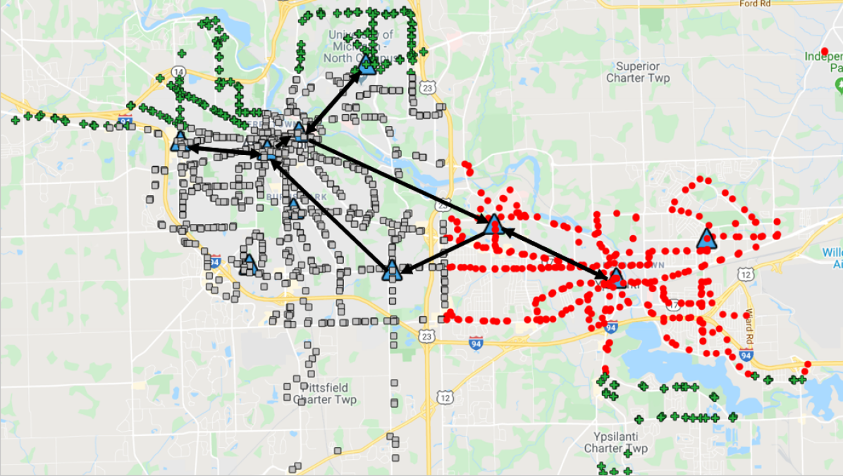
Figure 3: Network Design for the ODMTS with 10 Hubs (black triangles represent potential hub locations and black arrows show the open hub legs in the network design. In terms of bus stops; stops in low-income regions, middle-income regions, high-income regions correspond to red dots, gray squares, green pluses, respectively).

	Riders adopting ODMTS				Existing riders				Riders not adopting ODMTS
Income	ODMTS	direct	AAATA		ODMTS	direct	AAATA		ODMTS	direct	AAATA
low	NA				16.05	6.90	25.63		NA
medium	4.21	3.61	14.64		11.27	5.03	21.53		25.91	7.73	31.88
high	4.61	4.61	15.42		9.84	5.31	21.06		19.96	8.37	29.77

Table 2: Trip Duration Analysis under 10 Hubs Design.

	Riders adopting ODMTS				Existing riders				Riders not adopting ODMTS
Income	ODMTS	direct	AAATA		ODMTS	direct	AAATA		ODMTS	direct	AAATA
low	NA				18.39	6.91	25.63		NA
medium	3.21	2.82	12.19		14.16	5.03	21.53		27.38	7.23	29.14
high	4.47	4.47	14.42		10.41	5.36	21.06		21.09	8.37	29.99

Table 3: Trip Duration Analysis under 10 Hubs Design with Increased On-Demand Shuttle Cost.

Table 2 reports various statistics on trip durations per income level for existing riders, riders adopting the designed ODMTS, and those not adopting it. More precisely, the table uses the following classification: i) riders who choose to adopt the ODMTS, ii) existing riders of the transit system who have no mode choice and thus necessarily adopt the ODMTS, and iii) riders with choice who do not adopt the designed ODMTS. For each rider type and each income level, the table reports three average trip durations over the corresponding rider sets: the duration in the designed ODMTS, the duration of the direct trip, and the duration in the existing AAATA transit system.

The table highlights that the ODMTS routes are significantly shorter than those of the existing transit system. For existing riders, the trip durations reduced by 37%, 48%, and 53% for low-income, middle-income, and high-income riders. This is critical since many of these riders may not have an alternative transportation mean, and the ODMTS should not increase the travel time for the vast majority of these riders. In particular, out of 1503 trips, 1347 trips utilize the ODMTS as either their riders prefer adopting the ODMTS or they are part of the existing trips. From the set of trips with choice who adopt the ODMTS, all trips have a travel time which is less than their corresponding travel time in the current transit system. On the other hand, a subset of the existing trips have longer trip durations. Specifically, out of 1347 trips, 11% of trips (149 trips) have longer travel time in the ODMTS with on average 7.99 minutes longer trips. Note that this is a pessimistic estimate for the ODMTS as the transit times in the current system do not factor in the time to walk from the true origin to the bus stop and from bus stop to the true destination, whereas the ODMTS picks up and drops off the riders (essentially) at their origin and to their destination. This result demonstrates that, for 89% of the trips, ODMTS perform better compared to the current transit system with better convenience while being profitable at reasonable ticket prices as discussed in Section 6.2.7.

Furthermore, it is interesting to examine low-income riders whose trips take longer than 40 minutes in the existing transit system. These trips, called low-income long transit (LILT) trips, constitute 28% of the low-income rides and have an average transit time of 51.39 minutes. Under the baseline ODMTS design their average trip duration decreased to 32.21 minutes, a 37% reduction in transit time. For riders with mode choice, the durations of the existing transit routes are also significantly reduced under the baseline ODMTS design. Interestingly, riders who adopt the ODMTS have routes almost as short as direct trips. The reduction in average trip duration is 71% and 70% for middle-income and high-income riders who adopt the ODMTS design, making the proposed ODMTS substantially more attractive. The riders who do not adopt ODMTS have longer direct trip times: although the baseline ODMTS improves over the existing system, the reduction in transit time is not enough to induce a mode change.

6.2.2 Impact of Increased Cost for On-Demand Shuttles

Consider the case where the cost of on-demand shuttles increases by 50%. Figure 4 depicts the resulting ODMTS design which now opens all hubs and significantly increases their connectivity. The resulting ODMTS thus relies more on the bus network and less on the on-demand shuttles to serve the trips. The overall adoption rates decreased slightly, as 92% of the middle-income and 74% of the high-income riders adopt the system. This reduction in adoption is obviously directly linked to longer transit times. Table 3 reports the average trip durations corresponding to each rider class under this setting.

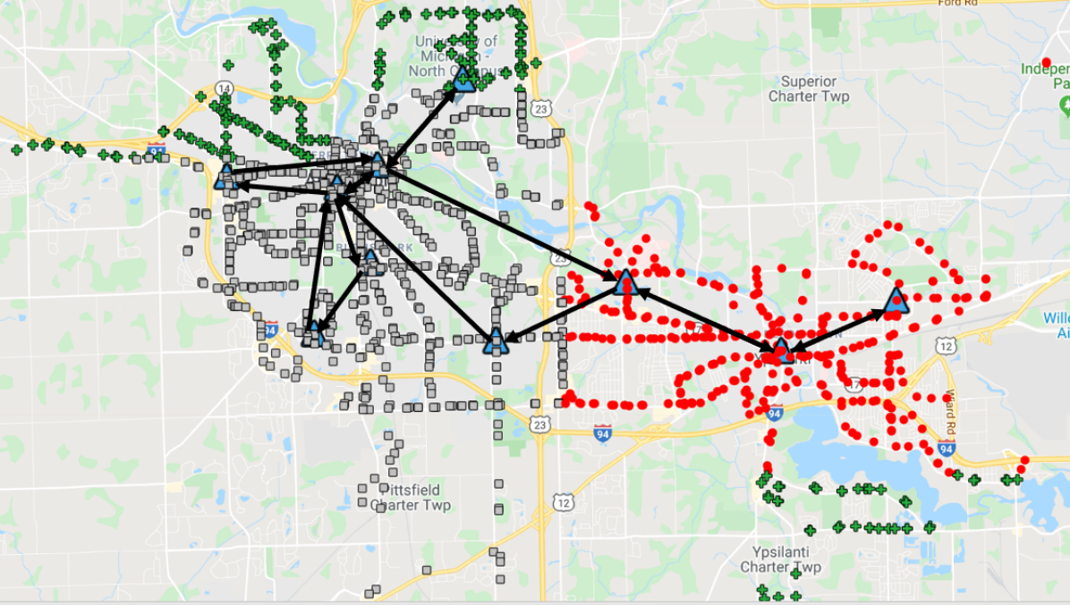
Figure 4: Network Design for the ODMTS with 10 Hubs with Increased On-Demand Shuttle Cost.

6.2.3 Impact of Weights of Cost and Inconvenience

This section studies the effect of the choice of the parameter $\theta$, which is used for adjusting the trade-off between cost and inconvenience in the weighted objective. It presents the results of the baseline instance in Section 6.2.1 under a higher value of $\theta$ as 0.01, i.e., giving more weight to inconvenience and less weight to cost of the ODMTS. The resulting network design is shown in Figure 5. Under this setting, in comparison to Figure 3, only three bus legs are open as the system aims at serving trips with shorter travel times, resulting in the usage of more on-demand shuttles. Table 4 summarizes the trip duration analysis under this setting, where 99% of middle-income and 100% of high-income riders adopt the ODMTS. As this ODMTS heavily depends on on-demand shuttles and do not benefit from the potential bus legs between hubs, it is not a desirable and sustainable system in comparison to the baseline setting with higher operational costs, as shown in Table 9. As larger $\theta$ values give similar results, $\theta$ is selected as 0.001 throughout the computational study.

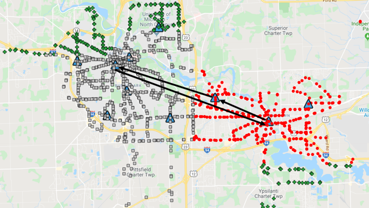
Figure 5: Network Design for the ODMTS with 10 Hubs with Increased $\theta$ parameter value.

	Riders adopting ODMTS				Existing riders				Riders not adopting ODMTS
Income	ODMTS	direct	AAATA		ODMTS	direct	AAATA		ODMTS	direct	AAATA
low	NA				8.47	6.70	25.63		NA
medium	5.75	5.16	21.65		5.76	4.93	21.53		31.99	15.03	70.52
high	6.98	6.79	24.69		5.17	5.13	21.06		NA

Table 4: Trip Duration Analysis under 10 Hubs Design with $\theta=0.01$.

6.2.4 Impact of Increased Ridership

This section examines the effect of increased ridership and studies the ODMTS design when the number of riders doubles. The resulting ODMTS design is illustrated in Figure 6. Again, all of the hubs are open and most of the bus legs from the baseline design also operate in the new design. Furthermore, the design increases connectivity to the lower-income communities by opening new bus legs in the corresponding regions. On the other hand, adoption ratios in terms of the trips decreased marginally: 92% of middle-income and 74% of high-income riders utilize the resulting system.

	Riders adopting ODMTS				Existing riders				Riders not adopting ODMTS
Income	ODMTS	direct	AAATA		ODMTS	direct	AAATA		ODMTS	direct	AAATA
low	NA				17.33	6.90	25.63		NA
medium	3.71	3.17	13.69		12.06	5.03	21.53		24.71	7.30	29.31
high	4.53	4.53	14.39		10.09	5.31	21.06		20.85	8.38	30.17

Table 5: Trip Duration Analysis under 10 Hubs Design with Doubled Ridership.

	Riders adopting ODMTS				Existing riders				Riders not adopting ODMTS
Income	ODMTS	direct	AAATA		ODMTS	direct	AAATA		ODMTS	direct	AAATA
low	32.40	11.99	51.50		13.01	5.65	19.07		49.24	10.05	50.46
medium	3.71	3.17	13.69		12.06	5.03	21.53		24.71	7.30	29.31
high	4.53	4.53	14.39		10.09	5.31	21.06		20.85	8.38	30.17

Table 6: Trip Duration Analysis under 10 Hubs Design with Doubled Ridership and Rider Choices for LILT trips.

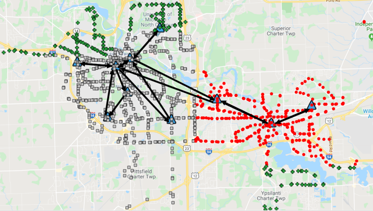
Figure 6: Network Design for the ODMTS with 10 Hubs with Doubled Ridership.

Table 5 presents the average trip durations for this design. Similar to the base case, the ODMTS performs better than the current transit system. The trip durations for existing riders become slightly longer in the new design as more bus legs are utilized.

6.2.5 Impact of Access Needs in ODMTS

The next results concern access to transit systems, a critical metric for transit agencies. As mentioned earlier, it is critical to ensure that low-income riders with no personal vehicles can be served by the transit system within reasonable transit times. Otherwise, they may lose their access to jobs, education, health-care, and other amenities, since the trip duration may become impractical. Consider again the LILT trips discussed in Section 6.2.1. To study these access needs to transit systems, these trip riders are associated with a choice model with $\alpha^{r}$ parameter set to 4. If a trip duration becomes longer than four times than the direct trip time, these riders will not be able to utilize the system anymore and lose access to major opportunities. Out of 476 low-income trips, there are 132 such LILT trips. The results are presented for the case of doubled ridership.

Under this model, 96% of low-income trips utilize the ODMTS system and almost all of the LILT riders adopt the ODMTS, demonstrating the system ability to meet access needs. The ODMTS design is the same as in Figure 6.

Table 6 presents the trip duration results with this choice model and doubled ridership. As the design remains the same, the middle-income and high-income trips have the same adoption rates and trip durations as in Table 5. LILT riders who adopt the ODMTS have an average trip duration less than three times that of the direct trip duration, and significantly shorter than the average trip duration by the existing transit system. On the other hand, LILT riders who do not adopt the ODMTS have much longer trip durations, although they have shorter trips on average compared to the current system. Figure 7 visualizes two of them, which are representative of trips for which riders do not adopt the ODMTS. The trips share the same destination (denoted by “de”) but have different origins (denoted by “or1” and “or2”). Their routes are illustrated with orange dashed routes from origins to destination. More specifically, the trip with origin “or1” uses an on-demand shuttle to reach the closest open hubs, but results in a long trip due to many transfers between hubs. On the other hand, the trip with origin “or2” utilizes the on-demand shuttles for longer trip segments, but it involves a transfer to the city center, increasing the trip duration. In general, however, all the LILT trips with destination points in the vicinity of the eastern-most hub adopt the ODMTS even when their origins are in the city center.

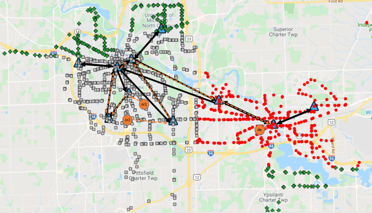
Figure 7: Visualization of Sample LILT Trips Not Adopting ODMTS.

6.2.6 Impact of Number of Hubs

It is also interesting to study the effect of increasing the number of hubs as ridership increases. Figure 8 presents the ODMTS design for 20 hubs and doubled ridership. The resulting design opens 14 hubs and the bus network has a significantly broader geographical coverage. In this setting, 91% of middle-income and 73% of high-income riders adopt the ODMTS respectively. Table 7 reports the average trip duration: the more expansive bus network induces increases of 11%, 18%, 1% in average trip durations for low-income, middle-income, and high-income riders respectively. Additionally, for the LILT trips, their average trip duration reduced from 51.39 minutes in the current transit system to 36.74 minutes in this setting, which is a 29% decrease on trip duration despite of having on average 2.5 minutes longer trips than the analogous ODMTS design for 10 hubs.

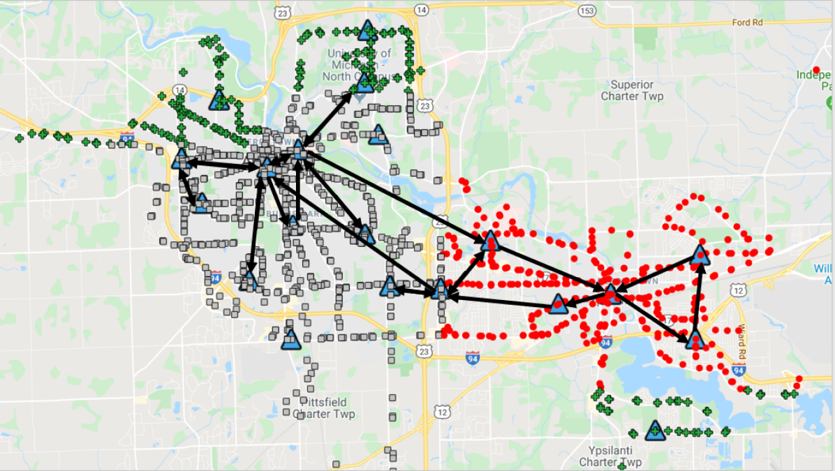
Figure 8: Network Design for the ODMTS with 20 Hubs with Doubled Ridership.

	Riders adopting ODMTS				Existing riders				Riders not adopting ODMTS
Income	ODMTS	direct	AAATA		ODMTS	direct	AAATA		ODMTS	direct	AAATA
low	NA				19.21	6.90	25.63		NA
medium	3.05	2.64	11.22		14.19	5.03	21.53		24.21	7.12	28.94
high	4.02	4.02	14.02		10.17	5.31	21.06		20.26	8.41	29.54

Table 7: Trip Duration Analysis under 20 Hubs Design with Doubled Ridership.

6.2.7 Adoption and Cost Analysis

Tables 8 and 9 present a detailed comparison of the ODMTS designs considered in Sections 6.2.1-6.2.6 with respect to the adoption, cost, and revenue. The revenue is assumed to be $2.5 per ride. 10Hub refers to the baseline design from Section 6.2.1, 10HubISC to the 10 hub design with increased on-demand shuttle costs from Section 6.2.2, 10HubMWI to the 10 hub design with more weight to minimizing inconvenience, 10HubDR to the 10 hub design with doubled ridership from Section 6.2.4, 10HubDRAC to the 10 hub design with doubled ridership and considerations of access from Section 6.2.5, and 20HubDR to the 20 hub design with doubled ridership from Section 6.2.6. In Table 8, columns “MI” and “HI” under “Adoption (%)” column represent the percentage of the middle and high income riders who adopt the ODMTS. No low-income riders have a choice model, except in 10HubDRAC where 3428 of 3508 low-income riders adopt the ODMTS. Column “# of Riders” corresponds to the number of riders considered in the design, with the number of riders utilizing the ODMTS in parentheses for middle-income, high-income and total riders, respectively. In Table 9, columns “Revenue”, “Inv Cost”, and “Trv Cost” represent the revenue of the transit agency (from existing users and those choosing to adopt the ODMTS), the investment cost of operating bus legs between hubs, and the total travel cost of the ODMTS riders. Column “Net Cost/Rider” presents the cost (or benefit) per rider: it is obtained by deducting the revenue from the sum of the investment and travel costs and dividing by the number of ODMTS riders.

	Adoption (%)			# of Riders
	MI	HI		MI	HI	Total
10Hub	94	74		3316 (3112)	722 (536)	5792 (5402)
10HubISC	92	74		3316 (3040)	722 (532)	5792 (5326)
10HubMWI	99	100		3316 (3312)	722 (722)	5792 (5788)
10HubDR	92	74		6632 (6124)	1444 (1068)	11584 (10700)
10HubDRAC	92	74		6632 (6124)	1444 (1068)	11584 (10620)
20HubDR	91	73		6632 (6052)	1444 (1048)	11584 (10608)

Table 8: Adoption Comparison under Different ODMTS Settings.

	Revenue & Costs
	Revenue	Inv Cost	Trv Cost	Net Cost/Rider
10Hub	13505.00	2440.80	13553.31	0.46
10HubISC	13315.00	3564.59	17516.07	1.46
10HubMWI	14470.00	1429.86	22153.77	1.57
10HubDR	26750.00	4073.14	23847.84	0.11
10HubDRAC	26550.00	4073.14	23642.55	0.11
20HubDR	26520.00	4959.34	20285.19	-0.12

Table 9: Cost and Revenue Comparison under Different ODMTS Settings.

The first interesting result is that the baseline design would be profitable for a price of $2.96, which is quite remarkable, given the improvements in quality of service and the increased ridership. Of course, the analysis ignores a variety of fixed costs and subsidies but the analysis reflects the significant ODMTS potential. As ridership grows, revenues also grow in proportion and the adoption rates remain similar. The investment cost for the bus network and the travel costs of the on-demand shuttles also grow but slower: this means that the net cost per rider decrease significantly, highlighting economies of scale in ODMTS. The 20-hub design is particularly interesting: the investment cost for the buses further increases but the cost for on-demand shuttles decreases more, making the ODMTS profitable at $2.5.

Capturing travel mode adoption in the design of ODMTS ensures that the transit system will be sized properly and have the targeted level of performance. However, it is also interesting to mention the financial benefits of modeling mode adoption. By scaling the obtained results for 52 weeks, 5 days a week, and 12 hours a day, the bilevel optimization model would produce savings of $165,937, $302,350, and $120,631 for 10HubDR, 20HubDR, and 10HubISC respectively.

6.3 Computational Efficiency

		10 hubs			20 hubs
Income	# of trips	direct trips	% Identified		direct trips	% Identified
low	476	145	30.46		106	22.27
medium	819	260	31.75		220	26.86
high	208	80	38.46		52	25.00
Total	1503	485	32.27		378	25.15

Table 10: Direct Trip Identification Analysis.

(a) 10 Hubs Instance.

(b) 20 Hubs Instance.

Figure 9: Impact of the Enhancements on Computational Performance.

This section reports a number of computational results on the bilevel optimization model, including the impact of the preprocessing steps and the valid inequalities. Table 10 reports on the ability to detect direct trips for instances with 10 and 20 hubs. 32% and 25% of the trips are identified as direct in the 10 hubs and 20 hubs instances. The percentage decreases for 20 hubs since the bus network is more expansive. In 10 hubs setting, the highest percentage of direct trips are high-income, as the hub locations are further away from the origin and destination of these trips. This percentage reduces substantially for 20 hubs for high-income class, especially in comparison to other rider classes, demonstrating the importance of hub locations and the number of hubs for this analysis.

Figures 9(a) and 9(b) examine the benefits of the bounds on the follower problem presented in Section 3.4.1 in combination with the valid inequalities proposed in Section 5.5 in comparison to a standard Benders decomposition algorithm with the nogood cuts for ensuring consistency between rider choices and network designs by excluding these enhancements. The figures use the baseline instance with 10 Hubs studied in Section 6.2.1 and the 20 Hubs instance studied in Section 6.2.6. They report the optimality gap and the run time at each iteration of the algorithm over a time limit of 1 hour and 10 hours for the 10 Hubs and 20 Hubs instances, which terminate with optimality gaps of %8.40 and %3.58 for the base case and %1.15 and %2.84 for the the enhanced case, respectively. Furthermore, under the same time limit, the base case and enhanced case are able to conduct 6 and 33 iterations for the 10 Hubs instance, and 22 and 26 iterations for the 20 Hubs instance. Note that 10 Hubs instance can be solved to optimality within 2 hours. The results demonstrate the significant computational impact of the bounds and valid inequalities: the proposed decomposition algorithm is capable of producing high-quality solutions in a reasonable amount of time for this real case study and brings improvements of several orders of magnitude compared to a decomposition algorithm that does not preprocess trips with respect to the bounds and only relies on Benders and classical nogood cuts.

As doubling the ridership in the case study considers the same origin-destination pairs with increased ridership amounts, the computational performance is not impacted by this change. On the other hand, increasing the number of distinct origin-destination pairs will typically impact the run time required for convergence of the solution algorithm. Table 11 highlights these results over instances with different trip sizes, which are randomly selected from the set of trips. It compares the runtimes of the algorithm when riders are all adopting the transit (no latent trips) and when some riders may adopt the system (latent trips) depending on the mode choice model, as discussed in Section 6.1. The results show how much more challenging the problem becomes when latent demand is taken into account. However, the algorithms presented in this paper, are still capable of addressing this planning problem and obtain small optimality gaps. This is significant, since latent demand is a key worry of transit agencies as mentioned in the introduction. Obviously, improved computational methods are an important topic for future research.

		10 hubs			20 hubs
# of trips	latent trips	# of iter.	run time (s)		# of iter.	run time (s)
100	No	2	4.96		2	9.91
	Yes	2	6.76		2	11.73
200	No	2	8.90		2	19.13
	Yes	3	14.12		3	24.66
500	No	5	50.58		5	94.96
	Yes	88	1316.76		94	18000.00*

Table 11: Run time comparison over instances with different trip sizes (*This instance reached the time limit with an optimality gap of %2.0).

7 Conclusion

This paper studied how to integrate rider mode preferences into the design of ODMTS. This functionality was motivated by the desire to capture the impact of latent demand, a key worry of transit agencies. The paper proposed a bilevel optimization model to address this challenge, in which the leader problem determines the ODMTS design, and the follower problems identify the most cost efficient and convenient route for riders under the chosen design. The leader model contains a choice model for every potential rider that determines whether the rider adopts the ODMTS given her proposed route.

To solve the bilevel optimization model, the paper proposed a decomposition method that includes Benders optimal cuts and nogood cuts to ensure the consistency of the rider choices in the leader and follower problems. Moreover, to improve the computational efficiency of the method, the paper proposed upper and lower bounds on trip durations for the follower problems and valid inequalities that strenghten the nogood cuts using the problem structure.

The paper also presented an extensive computational study on a real data set from AAATA, the transit agency for the broader Ann Arbor and Ypsilanti region in Michigan. The study considered the impact of a number of factors, including the price of on-demand shuttles, the number of hubs, and access to transit systems criteria. It analyzed the adoption rate of the ODTMS for various class of riders (low-income, middle-income, and high-income). The designed ODMTS feature high adoption rates and significantly shorter trip durations compared to the existing transit system both for existing riders and riders who adopted the ODMTS. Under increased ridership and/or the availability of more hubs, trip durations may increase as they use more bus legs between hubs and less on-demand shuttles; however, adoption rates are not impacted much and the net profit of the transit agency increases significantly through economies of scale. The results further highlighted the benefits in ensuring access for low-income riders as their trip durations decrease and remain reasonable. Finally, the computational study demonstrated the efficiency of the decomposition method for the case study and the benefits of computational enhancements.

Future work will consider more complex choice models (e.g., involving the increasing cost of transfers or probabilistic choice functions (Paneque et al. 2021)) and/or restrictions on acceptable routes. Scaling the approach to large metropolitan areas is also a priority.

Many thanks to Julia Roberts at AAATA for sharing the transit data and for many interesting discussions. This research is partly supported by NSF Leap HI proposal NSF-1854684, and Department of Energy Research Award 7F-30154.

8 Comparison with the Single-level Formulation

This section presents a single-level formulation for the bilevel problem in Figure 2 to demonstrate the need to adopt a bilevel approach. Figure 10 presents the single-level problem. which moves the constraints of the lower level problem to the upper level. For simplicity, the lexicographic objective in the follower problem is omitted.

$$\min_{z_{hl},x^{r}_{hl},y^{r}_{hl},b^{r},f^{r},\delta^{r}}\quad \sum_{h,l\in H}\beta_{hl}z_{hl}+\sum_{r\in T\setminus T^{\prime}}p^{r}b^{r}+\sum_{r\in T^{\prime}}p^{r}\delta^{r}(b^{r}-\varphi)$$ (23a)

s.t. $$\sum_{l\in H}z_{hl}=\sum_{l\in H}z_{lh}\quad\forall h\in H$$ (23b)

$$b^{r}=\sum_{h,l\in H}\tau_{hl}^{r}x_{hl}^{r}+\sum_{i,j\in N}\gamma_{ij}^{r}y_{ij}^{r}\quad\forall r\in T$$ (23c)

$$f^{r}=\sum_{h,l\in H}(t_{hl}+s)x_{hl}^{r}+\sum_{i,j\in N}t_{ij}y_{ij}^{r}\quad\forall r\in T$$ (23d)

$$\sum_{\begin{subarray}{c}h\in H\\ \text{if }i\in H\end{subarray}}(x_{ih}^{r}-x_{hi}^{r})+\sum_{j\in N}(y_{ij}^{r}-y_{ji}^{r})=\begin{cases}1&,\text{if }i=or^{r}\\ -1&,\text{if }i=de^{r}\\ 0&,\text{otherwise}\end{cases}\quad\forall i\in N,\>\forall r\in T$$ (23e)

$$x_{hl}^{r}\leq z_{hl}\quad\forall h,l\in H,\quad\forall r\in T$$ (23f)

$$\delta^{r}={\cal C}^{r}(\mathbb{x^{r}},\mathbb{y^{r}})\quad\forall r\in T^{\prime}$$ (23g)

$$z_{hl}\in\{0,1\}\quad\forall h,l\in H,\quad\delta^{r}\in\{0,1\}\quad\forall r\in T^{\prime}$$ (23h)

$$x_{hl}^{r}\in\{0,1\}\quad\forall h,l\in H,\quad y_{ij}^{r}\in\{0,1\}\quad\forall i,j\in N.$$ (23i)

Figure 10: The Single-level Optimization Model for ODMTS Design with Travel Mode Adoption.

The choice function of every trip $r$ depends on the trip durations $f^{r}$ as defined in (2). To represent this relationship, constraint (23g) can be linearized as follows:

$$f^{r} \geq\alpha^{r}t^{r}_{cur}+\epsilon_{f}-M_{f}\delta^{r},$$

$$f^{r} \leq\alpha^{r}t^{r}_{cur}+M_{f}(1-\delta^{r}),$$

where $\epsilon_{f}\approx 0$ and $M_{f}$ is an upper bound on all of the trip durations under any network design.

This formulation only evaluates the suggested routes and choices of the riders from the perspective of the transit agency, who consequently can suggest longer routes to the riders with choice if serving them is not profitable. Thus, their inconvenience is explicitly omitted in the system, which is undesirable for ensuring the access to the transit system.

To illustrate this potential behavior, this section presents a numerical study over the provided baseline setting in Section 6.2.1. The instance is built by randomly selecting 100 trips from the data set. For giving more riders the choice of adoption in this setting, all trips from low-income riders are considered as existing riders, whereas all trips from middle income and high income riders constitute the latent demand. Table 12 summarizes the comparison of the solutions of the bilevel problem in Figure 2 and the single-level problem in Figure 10 in terms of rider adoption. Since the single-level problem is a relaxation to the bilevel problem, it results in a smaller objective function value. However, the single-level problem has a much lower adoption for all riders with choice and it explicitly suggests longer routes to certain riders because serving them is not of direct benefit to the transit agency in terms of the objective function. This artificial removal of riders from the transit system also results in a different design with fewer opened bus legs.

These results highlight the need for the bi-level model in Figure 2 in order to eliminate this pathological and unfair behavior. This is aligned with the objectives of many transit agencies which aims at using ODMTS to improve mobility for underserved communities.

	# of trips (# of existing trips)	# of trips adopting ODMTS
		Single-level	Bilevel
low	34 (34)	34	34
medium	58 (0)	17	41
high	8 (0)	2	6

Table 12: Single-level and Bilevel models comparison over a sample instance.

9 Comparison with the Former Studies

This section expands the discussion presented in Section 3.3 to compare this study with the former study (Basciftci and Van Hentenryck 2020) in terms of the novel analytical results derived in Section 4, solution algorithm presented in Section 5 and case studies in Section 6. As the former paper studies an aligned choice model with the objective of the follower problem $b^{r}$, it benefits from the following result: Since the follower problem obtains the shortest path from origin to destination of a given trip with respect to the weighted cost and convenience of the arcs, $b^{r}$ value decreases as more hub legs become available. Then, the paper benefits from anti-monotone choice functions that are defined as follows.

Definition 9.1 (Anti-Monotone Mode Choice)

A choice function ${\cal C}^{r}$ is anti-monotone if $b^{r}_{1}\leq b^{r}_{2}\Rightarrow{\cal C}^{r}(b^{r}_{1})\geq{\cal C}^{r}(b^{r}_{2}).$

Observe that the choice function ${\cal C}^{r}(b^{r})\equiv\mathbbm{1}(b^{r}\leq\alpha^{r}\ b^{r}_{cur})$ is anti-monotone since $b_{1}^{r}\leq b_{2}^{r}$ implies ${\cal C}^{r}(b^{r}_{1})\geq{\cal C}^{r}(b^{r}_{2})$. Thus, to obtain the case $b_{1}^{r}\leq b_{2}^{r}$, we can simply consider evaluating $b^{r}$ under the designs $\mathbb{z}^{1}\geq\mathbb{z}^{2}$, where $b_{i}^{r}$ represents $b^{r}$ value under design $\mathbb{z}^{i}$. Under these relationships, nogood cuts (15) and (16) to ensure consistency between rider choices and design variables can be strengthened directly to the ones in (17) and (18) by adding or removing arcs from a given design, respectively, without deriving any further conditions. Having aligned objectives between the follower problem and the choice function along with the stronger cuts result in the fast convergence of the Benders decomposition based solution algorithm.

On the other hand, although the choice function studied in this paper is anti-monotone in terms of $f^{r}$, there is no direct relationship between the network design variable $z$ and the convenience $f^{r}$ as opening or closing of hub legs does not necessarily improve or deteriorate the convenience of the trips. Thus, the former results do not apply and these not aligned objectives complicate the solution procedure. To be able to strengthen the consistency cuts from nogood cuts in this setting, further analytical results are derived in Section 4. This analysis provides sufficient conditions to obtain the stronger cuts (17) and (18). Furthermore, to accelerate the solution algorithm, the problem size is reduced by identifying the direct trips derived through these analyses, as demonstrated in Table 10 over the studied instances. Moreover, stronger cuts in the form of (19) and (20) are derived by identifying certain hub legs whose addition or removal from a given design will not impact the convenience and consequently the adoption behavior of the riders. Furthermore, upper and lower bounds on the follower problem are presented in Section 3.4.1 to strengthen the presented formulation. The experiments demonstrate the significant computational benefits of adopting the proposed enhancements under this complicating setting with not aligned objectives.

In addition to the differences in the modelling perspectives discussed in Section 3.3 and these novel technical results tailored for this problem setting, this paper provides an extensive case study over the broader Ann Arbor and Ypsilanti area of Michigan over various instance settings. For each instance, the average trip time of each rider class depending on their adoption behaviour and income level are presented in comparison to the current transit system and direct travel option. The case study further presents results under different numbers of hubs, initial ridership amounts, on-demand shuttle costs, and with additional concerns on access to transit systems. These results demonstrate the performance of the ODMTS with high adoption percentages and better convenience along with profitability with reasonable ticket prices as ODMTS is designed under fixed pricing for existing riders and convenience concerned potential riders.

References

- Agatz et al. (2020) Agatz N, Hewitt M, Thomas BW (2020) “make no little plans”: Impactful research to solve the next generation of transportation problems. Networks 77(2):269–286.
- Alumur et al. (2012) Alumur S, Kara B, Karasan O (2012) Multimodal hub location and hub network design. Omega 40(6):927 – 939.