Nested Coordinate Systems in Geometric Algebra

Abstract

A nested coordinate system is a reassigning of independent variables to take advantage of geometric or symmetry properties of a particular application. Polar, cylindrical and spherical coordinate systems are primary examples of such a regrouping that have proved their importance in the separation of variables method for solving partial differential equations. Geometric algebra offers powerful complimentary algebraic tools that are unavailable in other treatments.

AMS Subject Classification MSC-2020: 15A63, 15A67, 42B37.

Keywords: Clifford algebra, coordinate systems, geometric algebra, separation of variables.

0 Introduction

Geometric algebra $\mathbb{G}_{3}$ is the natural generalization of Gibbs Heaviside vector algebra, but unlike the latter, it can be immediately generalized to higher dimensional geometric algebras $\mathbb{G}_{p,q}$ of a quadratic form. On the other hand, Clifford analysis, the generalization of Hamilton’s quaternions, is also expressed in Clifford’s geometric algebras [1]. The main purpose of this article is to formulate the concept of a nested coordinate system, a generalization of the well-known methods of orthogonal coordinate systems to apply to any coordinate system. We restrict ourselves to the geometric algebra $\mathbb{G}_{3}$ because of its close relationship to the Gibbs-Heaviside vector calculus [3]. This restriction also draws attention to the clear advantages of geometric algebra over the later, because of its powerful associative algebraic structure.

The idea of a nested rectangular coordinate system arises naturally when studying properties of polar coordinates in the $2$ and $3$-dimensional Euclidean vector spaces $\mathbb{R}^{2}$ and $\mathbb{R}^{3}$. We begin by discussing the relationship between ordinary polar coordinates and the nested rectangular coordinate system ${\cal N}_{1,2}$, before going on to the higher dimensional nested coordinate system ${\cal N}_{1,2,3}$ utilized in the reformulation of cylindrical and spherical coordinates. A detailed discussion of the geometric algebra $\mathbb{G}_{3}$ is not given here, but results are often expressed in the closely related well-known Gibbs-Heaviside vector analysis for the benefit of the reader.

1 Polar and nested coordinates systems

Let $\mathbb{G}_{2}:=\mathbb{G}(\mathbb{R}^{2})$ be the geometric algebra of $2$-dimensional Euclidean space $\mathbb{R}^{2}$. An introductory treatment of the geometric algebras $\mathbb{G}_{1}$, $\mathbb{G}_{2}$ and $\mathbb{G}_{3}$ is given in [4, 5, 6]. Most important in studying the geometry of the Euclidean plane is the position vector

$$\mathbf{x}:=\mathbf{x}[x,\hat{x}]=x\hat{x}$$ (1)

expressed here as a product of its Euclidean magnitude $x$ and its unit direction, the unit vector $\hat{x}$. In terms of rectangular coordinates $(x_{1},x_{2})\in\mathbb{R}^{2}$,

$$\mathbf{x}=\mathbf{x}[x_{1},x_{2}]=x_{1}e_{1}+x_{2}e_{2},$$ (2)

for the orthogonal unit vectors $e_{1},e_{2}$ along the $x_{1}$ and $x_{2}$ axis, respectively. The advantage of our notation is that it immediately generalizes to $3$ and higher dimensional spaces of arbitrary signature $(p,q)$ in any of the definite geometric algebras $\mathbb{G}_{p,q}:=\mathbb{G}(\mathbb{R}^{p,q})$ of a quadratic form.

The vector derivative, or gradient in the Euclidean plane is defined by

$$\nabla:=e_{1}\partial_{1}+e_{2}\partial_{2}$$ (3)

where $\partial_{1}:=\frac{\partial}{\partial x_{1}}$ and $\partial_{2}:=\frac{\partial}{\partial x_{2}}$ are partial derivatives [3, p.105]. Clearly,

$$e_{1}=\partial_{1}\mathbf{x}=e_{1}\cdot\nabla\mathbf{x},\ \ e_{2}=\partial_{2}\mathbf{x}=e_{2}\cdot\nabla\mathbf{x}.$$

Since $\nabla$ is the usual 2-dimensional gradient, it has the well-known properties

$$\nabla\mathbf{x}=2,\quad{\rm and}\quad\nabla x=\hat{x}.$$

With the help of the product rule for differentiation,

$$2=\nabla\mathbf{x}=(\nabla x)\hat{x}+x(\nabla\hat{x})=\hat{x}^{2}+x(\nabla\hat{x}).$$ (4)

Since in geometric algebra $\mathbf{x}^{2}=x^{2}$, it follows that $\hat{x}^{2}=1$, so that for $\mathbf{x}\in\mathbb{R}^{2}$,

$$\nabla\hat{x}=\frac{1}{x}\ \ {\rm and}\ \ e_{1}\cdot\nabla x=e_{1}\cdot\hat{x}=\frac{x_{1}}{x},\ \ e_{2}\cdot\nabla x=e_{2}\cdot\hat{x}=\frac{x_{2}}{x}.$$ (5)

Similarly, $\nabla\hat{x}=\frac{n-1}{x}$ for $\mathbf{x}\in\mathbb{R}^{n}$. This is the first of many demonstrations of the power of geometric algebra over standard vector algebra.

By a nested rectangular coordinate system ${\cal N}_{1,2}(x_{1},x[x_{1},x_{2}])$, we mean

$$\mathbf{x}=x\hat{x}=\mathbf{x}[x_{1},x]=\mathbf{x}\big{[}x_{1},x[x_{1},x_{2}]\big{]}.$$

The grouping of the variables allows us to consider $x_{1}$ and $x:=\sqrt{x_{1}^{2}+x_{2}^{2}}$ to be independent. The partial derivatives with respect to these independent variables is denoted by $\hat{\partial}_{1}:=\frac{\hat{\partial}}{\partial x_{1}}$ and $\hat{\partial}_{x}:=\frac{\hat{\partial}}{\partial x}$, the hat on the partial derivatives indicating the new choice of independent variables.

For polar coordinates $(x,\theta)\in\mathbb{R}^{2}$, for $x:=\sqrt{x_{1}^{2}+x_{2}^{2}}\geq 0$, $0\leq\theta<2\pi$, and $\mathbf{x}:=\mathbf{x}[x,\theta]$,

$$\mathbf{x}=x\hat{x}[\theta]=x(e_{1}\frac{x_{1}}{x}+e_{2}\frac{x_{2}}{x})=x(e_{1}\cos\theta+e_{2}\sin\theta),$$ (6)

where $\cos\theta:=\frac{x_{1}}{x}$ and $\sin\theta:=\frac{x_{2}}{x}$. Using (5),

$$\nabla\hat{x}=\nabla\hat{x}[\theta]=(\nabla\theta)\frac{\partial\hat{x}}{\partial\theta}=\frac{1}{x}\quad\iff\quad\nabla\theta=\frac{1}{x}\frac{\partial\hat{x}}{\partial\theta},\ \nabla^{2}\theta=0,$$ (7)

since

$$\nabla\hat{x}=(\nabla\theta)\partial_{\theta}(e_{1}\cos\theta+e_{2}\sin\theta)=(\nabla\theta)(-e_{1}\sin\theta+e_{2}\cos\theta),$$

and

$$\nabla^{2}\theta=-\frac{\hat{x}}{x^{2}}\partial_{\theta}\hat{x}+\frac{1}{x}(\nabla\theta)\partial_{\theta}^{2}\hat{x}=-2\Big{(}\frac{\hat{x}}{x^{2}}\cdot(\partial_{\theta}\hat{x})\Big{)}=0.$$

The $\iff$ follows by multipling both sides of the first equation by the unit vector $\partial_{\theta}\hat{x}$, which is allowable in geometric algebra. Note also the use of the famous geometric algebra identity $2\mathbf{a}\cdot\mathbf{b}=(\mathbf{a}\mathbf{b}+\mathbf{b}\mathbf{a})$ for vectors $\mathbf{a}$ and $\mathbf{b}$, [4, p.26].

The 2-dimensional gradient $\nabla$,

$$\nabla=e_{1}\frac{\partial}{\partial x_{1}}+e_{2}\frac{\partial}{\partial x_{2}}=e_{1}\partial_{1}+e_{2}\partial_{2}$$ (8)

already defined in (3), and the Laplacian $\nabla^{2}$ is given by

$$\nabla^{2}=\frac{\partial^{2}}{\partial x_{1}^{2}}+\frac{\partial^{2}}{\partial x_{2}^{2}}=\partial_{1}^{2}+\partial_{2}^{2}.$$ (9)

In polar coordinates,

$$\hat{\nabla}=(\nabla x)\hat{\partial}_{x}+(\nabla\theta)\hat{\partial}_{\theta}=\hat{x}\,\hat{\partial}_{x}+\frac{1}{x}(\hat{\partial}_{\theta}x)\hat{\partial}_{\theta}$$ (10)

for the gradient where $\hat{\partial}_{\theta}:=\frac{\hat{\partial}}{\partial\theta}$, and since $\hat{\nabla}^{2}\theta=0$,

$$\hat{\nabla}^{2}=\hat{\nabla}\big{(}\hat{x}\,\hat{\partial}_{x}+(\hat{\nabla}\theta)\,\hat{\partial}_{\theta}\big{)}=\Big{(}\hat{\nabla}\hat{x}+\hat{x}\cdot\hat{\nabla}\Big{)}\hat{\partial}_{x}+\Big{(}\hat{\nabla}^{2}\theta+(\hat{\nabla}\theta)\cdot\hat{\nabla}\Big{)}\hat{\partial}_{\theta}$$

$$=\hat{\partial}_{x}^{2}+\frac{1}{x}\hat{\partial}_{x}+\frac{1}{x^{2}}\hat{\partial}_{\theta}^{2}.$$ (11)

for the Laplacian. The decomposition of the Laplacian (11), directly implies that Laplace’s differential equation is separable in polar coordinates.

When expressed in nested rectangular coordinates ${\cal N}_{1,2}(x_{1},x)$, the gradient $\nabla\equiv\hat{\nabla}$ takes the form

$$\hat{\nabla}:=(\nabla x_{1})\frac{\hat{\partial}}{\partial x_{1}}+(\nabla x)\frac{\hat{\partial}}{\partial x}=e_{1}\hat{\partial}_{1}+\hat{x}\hat{\partial}_{x}.$$ (12)

Dotting equations (8) and (12) on the left by $e_{1}$ and $\hat{x}$ gives the transformation rules

$$\partial_{1}=\hat{\partial}_{1}+\frac{x_{1}}{x}\hat{\partial}_{x},\ \ \hat{x}\cdot\hat{\nabla}=\frac{x_{1}}{x}\hat{\partial}_{1}+\hat{\partial}_{x}=\cos\theta\,\partial_{1}+\sin\theta\,\partial_{2}.$$

Using these formulas the nested Laplacian takes the form

$$\hat{\nabla}^{2}=\hat{\partial}_{1}^{2}+2\frac{x_{1}}{x}\hat{\partial}_{x}\hat{\partial}_{1}+\frac{1}{x}\hat{\partial}_{x}+\hat{\partial}_{x}^{2}=-\hat{\partial}_{1}^{2}+2\partial_{1}\hat{\partial}_{1}+\frac{1}{x}\hat{\partial}_{x}+\hat{\partial}_{x}^{2}.$$ (13)

The unusual feature of the nested Laplacian is that it is defined in terms of both the ordinary partial derivative $\partial_{1}$ and the nested partial derivative $\hat{\partial}_{1}$. Whereas partial derivatives generally commute, partial derivatives of different types do not. For example, it is easily verified that

$$\partial_{1}\hat{\partial}_{1}x_{1}x^{2}=2x_{1},\ \ {\rm whereas}\ \ \hat{\partial}_{1}\partial_{1}x_{1}x^{2}=4x_{1}.$$

Because the mixed partial derivatives $\hat{\partial}_{x}\hat{\partial}_{1}$ occurs in (13), Laplace’s differential equation in the real rectangular coordinate system ${\cal N}_{1,2}(x_{1},x)$ is not, in general, separable. Indeed, suppose that a harmonic function $F$ is separable, so that $F=X_{1}X$ for $X_{1}=X_{1}[x_{1}],X=X[x]$. Using (13),

$$\frac{\hat{\nabla}^{2}F}{X_{1}X}=\frac{\partial_{1}^{2}X_{1}}{X_{1}}+\frac{\Big{(}\partial_{x}^{2}X+\frac{1}{x}\partial_{x}\Big{)}X}{X}+2\Big{(}\frac{x_{1}\partial_{1}X_{1}}{X_{1}}\Big{)}\Big{(}\frac{\partial_{x}X}{xX}\Big{)}=0.$$ (14)

The last term on the prevents F in general from being separable. However, it is easily checked that $F=k\frac{x_{1}}{x^{2}}$ is harmonic and a solution of (13). When $X_{1}[x_{1}]=kx_{1}$, it is easily checked that $\frac{x_{1}\partial_{1}X_{1}}{X_{1}}=1$. Letting $F=kx_{1}X[x]$, and requiring $\hat{\nabla}^{2}F=0$, leads to the differential equation for $X[x]$,

$$3\partial_{x}X+x\partial_{x}^{2}X=0,$$

with the solution $X[x]=c_{1}\frac{1}{x^{2}}+c_{2}$. The simplest example of a harmonic function $F=X_{1}X$ is when $X_{1}=x_{1}$ and $X=\frac{1}{x^{2}}$. A graph of this function is shown in Figure 1.

Figure 1: The harmonic $2$-dimensional function $F=\frac{x_{1}}{x_{1}^{2}+x_{2}^{2}}$ is shown.

2 Special harmonic functions in nested coordinates

Consider the real nested rectangular coordinate system $(x_{1},x_{p},x)$, defined by

$${\cal N}_{1,2,3}:=\{(x_{1},x_{p},x)|\ \mathbf{x}=x\hat{x}=x_{1}e_{1}+x_{p}\hat{x}_{p}+x\hat{x}\},$$

where $x_{p}=\sqrt{x_{1}^{2}+x_{2}^{2}}\geq 0,\ x=\sqrt{x_{1}^{2}+x_{2}^{2}+x_{3}^{2}}\geq 0$. In nested coordinates, the gradient $\nabla=e_{1}\partial_{1}+e_{2}\partial_{2}+e_{3}\partial_{3}$ takes the form

$$\hat{\nabla}=(\hat{\nabla}x_{1})\hat{\partial}_{1}+(\hat{\nabla}x_{p})\hat{\partial}_{p}+(\hat{\nabla}x)\hat{\partial}_{x}=e_{1}\hat{\partial}_{1}+\hat{x}_{p}\hat{\partial}_{p}+\hat{x}\hat{\partial}_{x},$$ (15)

where $\hat{\partial}_{p}:=\frac{\hat{\partial}}{\partial x_{p}}$. Formulas relating the gradients $\nabla$ and $\hat{\nabla}$ easily follow:

$$\partial_{1}=\hat{\partial}_{1}+e_{1}\cdot\hat{x}_{p}\,\hat{\partial}_{p}+e_{1}\cdot\,\hat{x}\,\hat{\partial}_{x}=\hat{\partial}_{1}+\frac{x_{1}}{x_{p}}\,\hat{\partial}_{p}+\frac{x_{1}}{x}\,\hat{\partial}_{x}$$ (16)

$$\partial_{2}=e_{2}\cdot\hat{x}_{p}\,\hat{\partial}_{p}+e_{2}\cdot\,\hat{x}\,\hat{\partial}_{x}=\frac{x_{2}}{x_{p}}\,\hat{\partial}_{p}+\frac{x_{2}}{x}\,\hat{\partial}_{x}$$ (17)

and

$$\partial_{3}=e_{3}\cdot\,\hat{x}\,\hat{\partial}_{x}=\frac{x_{3}}{x}\,\hat{\partial}_{x}.$$ (18)

For the Laplacian $\nabla^{2}$ in nested coordinates, with the help of (15),

$$\hat{\nabla}^{2}=\hat{\nabla}(e_{1}\hat{\partial}_{1}+\hat{x}_{p}\partial_{x_{p}}+\hat{x}\hat{\partial}_{x})=e_{1}\cdot\hat{\nabla}\,\hat{\partial}_{1}+\hat{\nabla}\cdot\hat{x}_{p}\,\hat{\partial}_{p}+\hat{\nabla}\cdot\hat{x}\,\hat{\partial}_{x}$$

$$=e_{1}\cdot\hat{\nabla}\,\hat{\partial}_{1}+\hat{\nabla}\cdot\hat{x}_{p}\,\hat{\partial}_{p}+\hat{\nabla}\cdot\hat{x}\,\hat{\partial}_{x}$$

$$=\Big{(}\hat{\partial}_{1}+\frac{x_{1}}{x_{p}}\,\hat{\partial}_{p}+\frac{x_{1}}{x}\,\hat{\partial}_{x}\Big{)}\hat{\partial}_{1}+\Big{(}\frac{1}{x_{p}}+\frac{x_{1}}{x_{p}}\hat{\partial}_{1}+\hat{\partial}_{p}+\frac{x_{p}}{x}\hat{\partial}_{p}\Big{)}\hat{\partial}_{p}$$

$$+\Big{(}\frac{2}{x}+\frac{x_{1}}{x}\hat{\partial}_{1}+\frac{x_{p}}{x}\hat{\partial}_{p}+\hat{\partial}_{x}\Big{)}\hat{\partial}_{x}$$

$$=\hat{\partial}_{1}^{2}+\hat{\partial}_{p}^{2}+\hat{\partial}_{x}^{2}+2\bigg{(}\frac{x_{1}}{x_{p}}\hat{\partial}_{1}\hat{\partial}_{p}+\frac{x_{1}}{x}\hat{\partial}_{1}\hat{\partial}_{x}+\frac{x_{p}}{x}\hat{\partial}_{p}\hat{\partial}_{x}\bigg{)}+\frac{1}{x_{p}}\hat{\partial}_{p}+\frac{2}{x}\hat{\partial}_{x}.$$ (19)

Another expression for the Laplacian in mixed coordinates is obtained with the help of (16),

$$\hat{\nabla}^{2}=-\hat{\partial}_{1}^{2}+\hat{\partial}_{p}^{2}+\hat{\partial}_{x}^{2}+2\bigg{(}\partial_{1}\hat{\partial}_{1}+\frac{x_{p}}{x}\hat{\partial}_{p}\hat{\partial}_{x}\bigg{)}+\frac{1}{x_{p}}\hat{\partial}_{p}+\frac{2}{x}\hat{\partial}_{x}.$$ (20)

Suppose $F=F[x_{1},x_{p},x]$. In order for $F$ to be harmonic, $\hat{\nabla}^{2}F=0$. Assuming that $F$ is separable, $F=X_{1}[x_{1}]X_{p}[x_{p}]X_{x}[x]$, and applying the Laplacian (20) to $F$ gives

$$\hat{\nabla}^{2}F=(\hat{\partial}_{1}^{2}X_{1})X_{p}X_{x}+X_{1}\Big{(}\big{(}\hat{\partial}_{p}^{2}+\frac{1}{x_{p}}\hat{\partial}_{p}\big{)}X_{p}\Big{)}X_{x}+X_{1}X_{p}\Big{(}\frac{2}{x}\hat{\partial}_{x}X_{x}\Big{)}$$

$$+2\bigg{(}\big{(}x_{p}\partial_{p}X_{p}\big{)}\big{(}\frac{1}{x}\hat{\partial}_{x}X_{x}\big{)}X_{1}+\big{(}\partial_{1}X_{p}\big{)}X_{x}+X_{p}\big{(}\partial_{1}X_{x}\big{)}\bigg{)}.$$ (21)

We now calculate the interesting expression

$$\frac{\big{(}x_{p}\partial_{p}X_{p}\big{)}\big{(}\frac{1}{x}\hat{\partial}_{x}X_{x}\big{)}X_{1}+\big{(}\partial_{1}X_{p}\big{)}X_{x}+X_{p}\big{(}\partial_{1}X_{x}\big{)}}{X_{1}X_{p}X_{x}}$$

$$=\Big{(}x_{p}\big{(}\partial_{p}\log X_{p}\big{)}\Big{)}\Big{(}\big{(}\frac{1}{x}\partial_{x}\log X_{x}\big{)}\Big{)}+\frac{\partial_{1}\log(X_{p}X_{x})}{X_{1}}.$$

In general, because of the last term in (21), a function $F=X_{1}X_{p}X_{x}$ will not be separable. However, just as in the two dimensional case, there are $3$-dimensional harmonic solutions of the form $F=x_{1}^{k}x_{p}^{m}x^{n}$. Taking the Laplacian (19) of $F$, with the help of [7], gives

$$\hat{\nabla}^{2}F=(2km+m^{2})x^{n}x_{1}^{k}x_{p}^{m-2}+(-k+k^{2})x^{n}x_{1}^{k-2}x_{p}^{m}$$

$$+(2kn+2mn+n(1+n))x^{n-2}x_{1}^{k}x_{p}^{m}=0.$$

This last expression vanishes when the system of three equations,

$$\{2km+m^{2}=0,\ \ -k+k^{2}=0,\ \ {\rm and}\ \ 2kn+2mn+n(1+n)=0\}.$$

All of the distinct non-trivial harmonic solutions $F=x_{1}^{k}x_{p}^{m}x^{n}$ are listed in the following Table

k m n

1 0 0

0 0 -1

1 -2 0

1 0 -3

1 -2 1

(22)

3 Cylindrical and spherical coordinates

Cylindrical and spherical coordinates are examples of nested coordinates ${\cal N}_{1,2}(\mathbb{R})$, and ${\cal N}_{2,3}(\mathbb{R})$, respectively. For the first,

$$\mathbf{x}=\mathbf{x}[x_{p},\theta,x_{3}]=\mathbf{x}_{p}[x_{p},\theta]+\mathbf{x}_{3}[x_{3}],$$ (23)

where $\mathbf{x}_{p}=x_{p}\hat{x}_{p}[\theta]$, $x_{p}=\sqrt{x_{1}^{2}+x_{2}^{2}}$, and $\mathbf{x}_{3}=x_{3}e_{3}$. Cylindrical coordinates $(x_{p},\theta,x_{3})\in\mathbb{R}^{3}=\mathbb{R}^{2}\cup\mathbb{R}^{1}$ are a decomposition of $\mathbb{R}^{3}$ into the polar coordinates $(x_{p},\theta)\in\mathbb{R}^{2}$, already studied in Section 1, and $x_{3}\in\mathbb{R}^{1}$. For spherical coordinates, $\mathbf{x}_{p}=x_{p}\hat{x}_{p}[\theta]$ the same as in cylindrical and polar coordinates, and

$$\mathbf{x}=\mathbf{x}[x,\theta,\varphi]=x\hat{x}[\theta,\varphi])=x\Big{(}e_{3}\cos\varphi+\hat{x}_{p}[\theta]\sin\varphi\Big{)},$$ (24)

where

$$x=\sqrt{x_{1}^{2}+x_{2}^{2}+x_{3}^{2}},\ \hat{x}[\theta,\varphi]=e_{3}\cos\varphi+\hat{x}_{p}[\theta]\sin\varphi,\ \hat{x}_{p}[\theta]=e_{1}\cos\theta+e_{2}\sin\theta.$$

The basic quantities that define both cylindrical and spherical coordinates are shown in Figure 2.

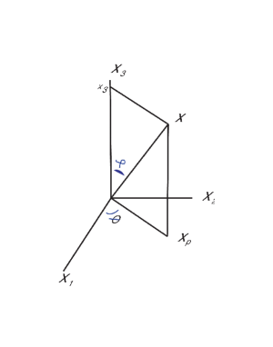
Figure 2: For cylindrical coordinates, $\mathbf{x}=x_{p}\hat{x}_{p}[\theta]+x_{3}e_{3}$. For spherical coordinates, $\mathbf{x}=x(e_{3}\cos\varphi+\hat{x}_{p}[\theta]\sin\varphi)$.

The gradient $\hat{\nabla}$ and Laplacian $\hat{\nabla}^{2}$ for cylindrical coordinates are easily calculated. With the help of (7), (10), and (11),

$$\hat{\nabla}=(\hat{\nabla}x_{p})\hat{\partial}_{p}+(\hat{\nabla}\theta)\hat{\partial}_{\theta}+(\hat{\nabla}x_{3})\hat{\partial}_{3}$$

for the cylindrical gradient, and

$$\hat{\nabla}^{2}=\hat{\nabla}\Big{(}\hat{x}_{p}\,\hat{\partial}_{p}+(\hat{\nabla}\theta)\,\hat{\partial}_{\theta}+e_{3}\hat{\partial}_{3}\Big{)}=\hat{\partial}_{p}^{2}+\frac{1}{x_{p}}\hat{\partial}_{p}+\frac{1}{x_{p}^{2}}\hat{\partial}_{\theta}^{2}+\hat{\partial}_{3}^{2}$$ (25)

for the cylindrical Laplacian. Letting $F[\mathbf{x}]=X_{p}[x]X_{\theta}[\theta]X_{3}[x_{3}]$, the resulting equation is easily separated and solved by standard methods, resulting in three second order differential equations with solutions,

$$X_{p}[x_{p}]=k_{1}J_{n}[\beta x_{p}]+k_{2}Y_{n}[\beta x_{p},]$$

$$X_{\theta}[\theta]=k_{3}\cos n\theta+k_{4}\sin n\theta$$

$$X_{3}[x_{3}]=k_{5}\cosh(\alpha(m-x_{3}))+k_{6}\sinh(\alpha(m-x_{3})),$$

where $J_{n}$ and $Y_{n}$ are Bessel functions of the first and second kind . The constants are determined by the various boundary conditions that must be satisfied in different applications [8, p.254].

Turning to spherical coordinates $(x,\theta,\varphi)\in\mathbb{R}^{3}$, the spherical gradient

$$\hat{\nabla}=(\hat{\nabla}x)\hat{\partial}_{x}+(\hat{\nabla}\theta)\hat{\partial}_{\theta}+(\hat{\nabla}\varphi)\hat{\partial}_{\varphi}=\hat{x}\hat{\partial}_{x}+\frac{1}{x_{p}}(\hat{\partial}_{\theta}\hat{x}_{p})\hat{\partial}_{\theta}+\frac{1}{x}(\hat{\partial}_{\varphi}\hat{x})\hat{\partial}_{\varphi},$$ (26)

where from previous calculations for polar and cylindrical coordinates,

$$\hat{\nabla}\theta=\frac{1}{x_{p}}(\hat{\partial}_{p}\hat{x}_{p}),\ (\hat{\nabla}\theta)^{2}=\frac{1}{x_{p}^{2}},\ \ \hat{\nabla}^{2}\theta=0,\ \ \hat{\nabla}\varphi=\frac{1}{x}\hat{\partial}_{\varphi}\hat{x},\ \ (\hat{\nabla}\varphi)^{2}=\frac{1}{x^{2}}.$$ (27)

Furthermore, since $\hat{x}=\hat{x}[\theta,\varphi]=e_{3}\cos\varphi+\hat{x}_{p}[\theta]\sin\varphi$

$$\frac{2}{x}=\hat{\nabla}\hat{x}=(\hat{\nabla}\theta)(\hat{\partial}_{\theta}\hat{x})+(\hat{\nabla}\varphi)(\hat{\partial}_{\varphi}\hat{x})=\frac{1}{x_{p}}(\hat{\partial}_{\theta}\hat{x})(\hat{\partial}_{\varphi}\hat{x})+\frac{1}{x},$$

it follows that

$$(\hat{\partial}_{\theta}\hat{x})(\hat{\partial}_{\varphi}\hat{x})=\frac{x_{p}}{x}=\sin\varphi,\ \ {\rm and}\ \ \hat{\nabla}^{2}\varphi=\frac{x_{3}}{x^{2}x_{p}}.$$

That $\hat{\nabla}^{2}\varphi=\frac{x_{3}}{x^{2}x_{p}}$ follows using (26) and (27),

$$\hat{\nabla}^{2}\varphi=\hat{\nabla}\big{(}\frac{1}{x}\hat{\partial}_{\varphi}\hat{x}\big{)}=\Big{(}-\frac{\hat{x}}{x^{2}}+\frac{1}{x}\hat{\nabla}\Big{)}\hat{\partial}_{\varphi}\hat{x}$$

$$=-\frac{\hat{x}}{x^{2}}\hat{\partial}_{\varphi}\hat{x}-\frac{1}{x}\Big{(}(\hat{\nabla}x)\hat{\partial}_{x}\hat{\partial}_{\varphi}\hat{x}+(\hat{\nabla}\theta)\hat{\partial}_{\theta}\hat{\partial}_{\varphi}\hat{x}+(\hat{\nabla}\varphi)\hat{\partial}_{\varphi}^{2}\hat{x}\Big{)}$$

$$=-\Big{(}\frac{\hat{x}}{x^{2}}\hat{\partial}_{\varphi}\hat{x}+\frac{1}{x^{2}}(\hat{\partial}_{\varphi}\hat{x})\hat{x}\Big{)}+\frac{1}{xx_{p}}(\hat{\partial}_{\theta}\hat{x}_{p})(\hat{\partial}_{\varphi}\hat{\partial}_{\theta}x)=\frac{x_{3}}{x^{2}x_{p}},$$

since partial derivatives commute, $\hat{\partial}_{x}\hat{x}=0$, and $\hat{\partial}_{\varphi}^{2}\hat{x}=-\hat{x}$.

For the spherical Laplacian, using (26) and (27),

$$\hat{\nabla}^{2}=\hat{\nabla}\Big{(}\hat{x}\hat{\partial}_{x}+(\hat{\nabla}\theta)\hat{\partial}_{\theta}+(\hat{\nabla}\varphi)\hat{\partial}_{\varphi}\Big{)}$$

$$=\Big{(}\frac{2}{x}+\hat{\partial}_{x}\Big{)}\hat{\partial}_{x}+(\hat{\nabla}\theta)\cdot\hat{\nabla}\hat{\partial}_{\theta}+\Big{(}\hat{\nabla}^{2}\varphi+(\hat{\nabla}\varphi)\cdot\hat{\nabla}\Big{)}\hat{\partial}_{\varphi}$$

$$=\Big{(}\hat{\partial}_{x}+\frac{2}{x}\Big{)}\hat{\partial}_{x}+\frac{1}{x_{p}^{2}}\hat{\partial}_{\theta}^{2}+\Big{(}\frac{x_{3}}{x^{2}x_{p}}+\frac{1}{x^{2}}\hat{\partial}_{\varphi}\Big{)}\hat{\partial}_{\varphi},$$

equivalent to the usual expression for the Laplacian in spherical coordinates [8, p.256].

Just as in cylindrical coordinates, the solution of Laplace’s equation in spherical coordinates is separable, $F=X_{x}[x]X_{\theta}[\theta]X_{\varphi}[\varphi]$, resulting in three second order differential equations with solutions

$$X_{x}[x]=k_{1}x^{\beta}+k_{2}x^{-(\beta+1)},$$

$$X_{\theta}[\theta]=k_{3}\cos n\theta+k_{4}\sin n\theta,$$

$$X_{\varphi}[\varphi]=k_{5}P_{n}^{m}(\cos\varphi)+k_{6}Q_{n}^{m}(\cos\varphi),$$

where $P_{n}^{m}$ and $Q_{n}^{m}$ are the Legendre functions of the first and second kind, respectively [8, p.258].

References

[1] R. Ablamowicz, G. Sobczyk, Editors: Lectures on Clifford (Geometric) Algebras and Applications, Birkhäuser, Boston 2003.
[2] E. Hobson, 1931, The theory of spherical and ellipsoidal harmonics,
Cambridge.
[3] J.E. Marsden, A.J. Tromba, Vector Calculus 2nd Ed., Freeman and Company, San Francisco 1980.
[4] G. Sobczyk, Matrix Gateway to Geometric Algebra, Spacetime and Spinors, Independent Publisher November 2019. https://www.garretstar.com
[5] G. Sobczyk, New Foundations in Mathematics: The Geometric Concept of Number,
Birkhäuser, New York 2013.
[6] G. Sobczyk. Many early versions of my work can be found on arXiv, or on my website: https://www.garretstar.com
[7] S. Wolfram, Mathematica.
[8] Tyn Myint-U, Partial Differential Equations of Mathematical Physics 2nd Ed., North Holland, NY 1980.