Markov models of coarsening in two-dimensional foams with edge rupture

Abstract

We construct Markov processes for modeling the rupture of edges in a two-dimensional foam. We first describe a network model for tracking topological information of foam networks with a state space of combinatorial embeddings. Through a mean-field rule for randomly selecting neighboring cells of a rupturing edge, we consider a simplified version of the network model in the sequence space $\ell_{1}(\mathbb{N})$ which counts total numbers of cells with $n\geq 3$ sides ($n$-gons). Under a large cell limit, we show that number densities of $n$-gons in the mean field model are solutions of an infinite system of nonlinear kinetic equations. This system is comparable to the Smoluchowski coagulation equation for coalescing particles under a multiplicative collision kernel, suggesting gelation behavior. Numerical simulations reveal gelation in the mean-field model, and also comparable statistical behavior between the network and mean-field models.

Keywords: foams, kinetic equations, Markov processes, combinatorial embeddings

Mathematics Subject Classification: 82D30,37E25,60J05

1 Introduction

Foams are a common instance of macroscopic material structure encountered in manufacturing. Some foams are desirable, such as those found in mousses, breads, detergents, and cosmetics, while others are unwanted byproducts in the production of steel, glass, and pulp [29, 7]. To better understand the complex geometric and topological structure of three-dimensional foams, scientists have designed simplified experiments to create two-dimensional foams, often through trapping a soap foam in a region between two transparent plates thin enough for only a single layer of cells to form [6, 16, 10, 27].

To replicate the topological transition that we find in an edge rupture, the author has conducted a simple experiment with a soap foam consisting of a mixture of liquid dish soap and water. The mixture is vigorously stirred to produce a foam and then spooned onto a $28\times 36\times.3$ cm transparent acrylic plate. Another plate is placed on top of the foam and then compressed to form a two-dimensional structure. The plates are tilted vertically to drain liquid, and after several minutes the foam sufficiently dries into a structure approximating a planar network. To produce the transition seen in Fig. 1, a small local force is applied to the outside of a plate at the center of an edge, causing it to rupture, immediately followed by each of the two neighboring edges at the rupturing edge’s endpoints merging into a single edge . While the experiment just described selects a single edge for rupture, multiple ruptures can occur naturally without applying external forces, with a typical time scale for the coarsening of the foam on the order of tens of minutes [8]. The rupture rate can be increased through using a weaker surfactant or applying heat. Typically, periods between ruptures are nonuniform, with infrequent ruptures eventually turning into a cascading regime during which the majority of ruptures occur [27].

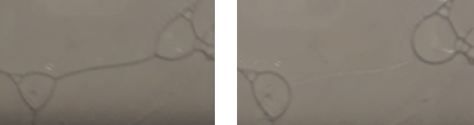
Figure 1: An edge in a two-dimensional soap foam immediately before (left) and after (right) its rupture. The length of the edge before rupture is approximately $1$ cm. 

The focus for this work is to construct minimal Markovian models for studying the statistical behavior of two-dimensional foams which coarsen through multiple ruptures of the type seen in Fig. 1. As a basis for comparison, let us briefly overview the more well-studied coarsening process of gas diffusion across cell boundaries. For a foam with isotropic surface tension on its boundary, gas diffusion induces network edges to evolve with respect to mean curvature flow. In two dimensions, the $n-6$ rule of von Neumann and Mullins [28, 23] gives a particularly elegant result that area growth of each cell with $n$ sides is constant and proportional to $n-6$. A cell with fewer than six sides can therefore shrink to a point, triggering topological changes in its neighboring cells. Several physicists used the $n-6$ rule to write down kinetic limits in the form of transport equations with constant area advection and a nonlinear intrinsic source term for handling topological transitions. Simulations of these models were shown to produce universal statistics found in physical experiments and direct numerical simulations on planar networks [14, 20, 15, 19].

The time scale for coarsening by gas diffusion is much slower than edge rupture, and is often measured in tens of hours [8]. In a foam with rupture, gas diffusion is a relatively minor phenomenon in determining densities for numbers of sides, and our models for this study will not consider diffusion by coarsening. Furthermore, the repartitioning of areas for cells after a rupture is a complex event where edges quickly adjust to reach a quasistationary state to minimize total surface tension, and unfortunately there is no known analog of the $n-6$ rule relating area and cell topology for ruptures. Since a main theme in this paper is to keep our models minimal, we will avoid questions related to cell areas, but rather only study frequencies of $n$-gons (cells with $n$ sides) after a total number of ruptures are performed. In Section 2, we construct a Markov chain model over a state space of combinatorial embeddings, which we refer to as ‘the network model’. Correlations in space between which two edges rupture in succession have been observed in physical experiments [6]. However, Chae and Tabor [8, Sect. IV:A] performed numerical simulations on several random models of foam rupture with uncorrelated rules for selecting rupturing edges, including selecting edges with uniform probability, and found comparable long-term behavior to physical experiments. In particular, all models produced networks consisting of larger cells surrounded by many smaller cells having few sides.

Using combinatorial rather than geometric embeddings as a state space in the network model allows us to track topological information of a network without needing to record geometrical quantities such as edge length, vertex coordinates, or curvature. A state transitions by removing a random edge from the network and performing the smoothing operation seen in Fig. 1. Explicit expressions for state transitions are provided in Section 2.3. While the network model does not need any geometric information to be well-defined, it is possible to generate a visualization of the coarsening process if we are provided with vertex coordinates for an initial embedding. Snapshots of the Markov chain $\{\mathbf{G}(m)\}_{m\geq 0}$ after $m=250k$ ruptures for $k=1,\dots,8$ are given in Figs. 2 and 3 for foams having initial conditions of 2500 cells generated by a randomly seeded Voronoi diagram and hexagonal lattice.

A schematic of the changes in side numbers for cells adjacent to a rupturing edge is given in Fig. 4. Typically, edge rupture can be seen as the composition of two graph operations:

1. Face merging: The two cells whose boundaries completely contain the rupturing edge will join together as a single cell after rupture. If the two cells have $i$ and $j$ sides before rupture, the new cell created from face merging has $i+j-4$ sides.

2. Edge merging: Each of the two cells sharing only a single vertex with the rupturing edge will have two of its edges smooth to create a single edge. If the two cells have $k$ and $l$ sides before rupture, the cells after edge merging have $k-1$ and $l-1$ sides.

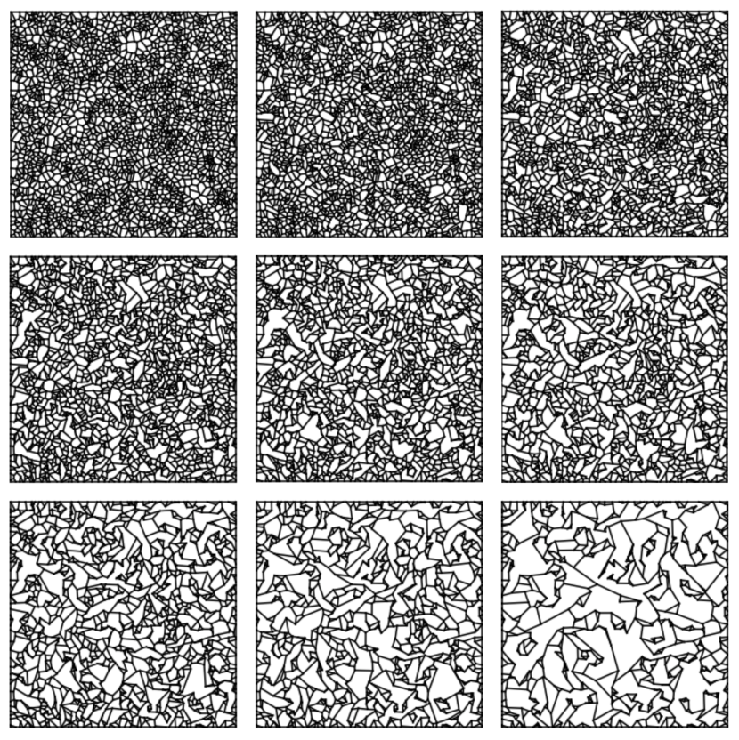
Figure 2: Snapshots of a sample path $\{\mathbf{G}(m)\}_{m\geq 0}$ with disordered initial conditions of a Voronoi diagram with random seeding. Top row left to right: $\mathbf{G}(0),\mathbf{G}(250),$ and $\mathbf{G}(500)$. Middle row: $\mathbf{G}(750),\mathbf{G}(1000),$ and $\mathbf{G}(1250)$. Bottom row: $\mathbf{G}(1500),\mathbf{G}(1750),$ and $\mathbf{G}(2000)$.  

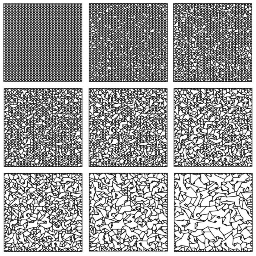
Figure 3: Snapshots of a sample path $\{\mathbf{G}(m)\}_{m\geq 0}$ with ordered hexagonal lattice initial conditions. Top row left to right: $\mathbf{G}(0),\mathbf{G}(250),$ and $\mathbf{G}(500)$. Middle row: $\mathbf{G}(750),\mathbf{G}(1000),$ and $\mathbf{G}(1250)$. Bottom row: $\mathbf{G}(1500),\mathbf{G}(1750),$ and $\mathbf{G}(2000)$.

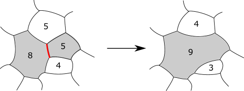
Figure 4: Side numbers immediately before (left) and after (right) a typical edge rupture. A numbers inside a cell denotes its number of sides. The rupturing edge is shown in bold red. Shaded cells denote those which undergo face merging.

In Fig. 4, shaded cells with eight and five sides merge to form a cell with nine sides, and the two unshaded cells with five and four sides undergo edge merging, producing cells with four and three sides. For a cell $C_{n}$ containing $n$ sides, we represent edge rupture with the three irreversible reactions

$$C_{i}+C_{j}\rightharpoonup C_{i+j-4},\quad C_{k}\rightharpoonup C_{k-1},\quad C_{l}\rightharpoonup C_{l-1}.$$ (1)

Rupture is mentioned as an ‘elementary move’ in [17] and [8] along with reactions occurring from gas diffusion, although the reaction (1) is not explicitly written down. It is important to note that not all ruptures will produce the reactions in (1). For instance, some edges do not have four distinct cells as neighbors. As an example, the ‘isthmus’ shown Fig. 5 has only three neighbors. To further complicate matters, rupture causes a loss of numbers of sides in neighboring cells which can create loops, multiedges, and islands. To keep our model minimal, in Section 2.2 we define a class rupturable edges which restricts all reactions to satisfy (1), with the exception of some edges at the domain boundary which have a similar reaction. Appendix A is meant to explicitly show the variety of reactions which can occur when some of the conditions for rupturable edges are lifted. Section 2.3 shows that the rupture operations restricted to rupturable edges is closed in a suitably chosen space of combinatorial embeddings. This enables us to construct a well-defined Markov chain by randomly selecting edges to rupture at each transition.

A major advantage of keeping the network model minimal is the relative ease of creating a simplified mean-field Markov model to approximate statistical topologies. In Section 3, we define a mean-field rule and its associated Markov chain for randomly selecting neighbors of a rupturing edge which only depends on $n$-gon frequencies. A formal argument for deriving kinetic equations in the large particle limit of the mean-field model is given in Section 4. The limiting equations give number densities $u_{n}(t)$ of $n$-gons, with a time scale $t\geq 0$ of the fraction of edge ruptures over the initial number of cells. The kinetic equations take the form of the nonlinear autonomous system

$$\dot{u}_{n} =\sum_{i=3}^{n+1}K^{F}_{4+n-i,i}u_{4+n-i}u_{i}+2q_{n+1}^{E}u_{n+1}-2q_{n}^{F}u_{n}-2q_{n}^{E}u_{n},\quad n\geq 3.$$ (2)

The terms $K^{F},q^{F},$ and $q^{E}$ are state-dependent rates of creation and annihilation of $n$-gons through face and edge merging. We derive explicit formulas for these rates in Section 4.

We note the similarity of (2) to the Smoluchowski coagulation equation [24] for number densities $v_{n}$ of size $n$ coalescing clusters, given by

$$\dot{v}_{n}=\frac{1}{2}\sum_{i=1}^{n-1}K_{n-i,i}v_{n-i}v_{i}-\sum_{i\geq 1}K_{n,i}v_{n}v_{i},\quad n\geq 1.$$ (3)

A major result for the Smoluchowski equations is the decrease of the total mass $\sum_{k\geq 1}kv_{k}$ under the multiplicative kernel $K_{i,j}=ij$ [21]. The missing total number is interpreted as a gel, or a single massive particle of infinite mass. In (2), we find that the rate of cell merging between $i$ and $j$-gons is

$$K^{F}_{i,j}=\frac{ij}{S^{2}(1-p_{3}^{2})},\quad S=\sum_{k\geq 3}ku_{k},\quad p_{3}=3u_{3}/S.$$

The similarity between $K^{F}_{i,j}$ and $K_{i,j}$ suggests the formation of a gel in (2), which should be interpreted as a cell with infinitely many sides.

In Section 5, we perform Monte Carlo numerical simulations of edge ruptures over large networks for both the network and mean-field models. The large initial cell number produces number densities which are approximately deterministic (having low variance at all times). For the mean-field model, we find strong evidence of gelation behavior. While we find that topological frequencies between the mean-field and network models generally agree to within a few percentage points, we observe that gelation behavior is quite weak in the network model. We conjecture that this is likely due to the rupturability requirements imposed in Def. 6.

As the kinetic equations for (2) only give interactions between cells with finitely many sides (the sol), we should interpret that the mean-field model approximates (2) only in the pregelation phases. The postgelation regime will require separate kinetic equations which include interactions of the sol with the gel. An advantage to Monte Carlo simulations is that they are a relatively simple method for approximating limiting number densities in both regimes, as opposed to the numerics involved in a deterministic discretization of the infinite system (2) (see [12] for a finite volume method for simulating coagulation equations). We hope to produce a more rigorous numerical and theoretical treatment of the phase transition in future works.

2 The network model

In this Section, we construct a minimal Markovian model, referred to as the ‘network model’, for tracking topological information of foams.

2.1 Foams as planar embeddings

We begin our construction of the network model by defining geometric embeddings which model two-d foams. Our space of embeddings is chosen to capture the typical topological reaction (1) seen in physical foams while also being sufficiently minimal to permit a derivation of limiting kinetic equations.

Definition 1.

The space of simple foams $\mathfrak{M}(S)$ in the unit square $S=[0,1]^{2}$ is the set of planar embeddings $\widetilde{G}\subset S$ of a simple connected trivalent planar graph $G$ such that $\widetilde{G}$ contains the boundary $\partial S.$

Some comments are in order for our choice of embeddings. We first mention that the ambient space $S$ can certainly be generalized to other subsets of the plane or a two-dimensional manifold. However, restricting to the unit square is a natural choice since previous physical experiments involve generating foams between two rectangular glass panes, and numerical simulations generating foams are often performed on rectangular domains [6, 16, 10, 27]. We also require that the boundary $\partial S$ is contained in the graph embedding so that the collection of cells covers all of $S$. Edges contained in $\partial S$ are considered as walls, and are not allowed to rupture. We do, however, allow rupture of edges with one or both vertices on $\partial S$. The reaction equations for these ruptured edges are slightly different than (1), as there is no cell adjacent to the vertex which undergoes edge merging.

Requiring $G$ to be trivalent is a consequence of the Herring conditions [18] for isotropic networks, which can be derived through a force balance argument. Connected and simple graphs are imposed for keeping the model minimal. Connectivity allows for us to represent all sides in a cell with a single directed loop. Simple graphs forbid loops and multiedges, which in graph embeddings are one and two-sided cells. To prevent the creation of 2-gons we will require reactants in (1) to contain sufficiently many sides.

For a planar embedding $\widetilde{G}\subset S$ of a graph $G$, we can represent faces using counterclockwise vertex paths $\sigma=(v_{1},\dots,v_{n})$, where $\{v_{i},v_{i+1}\}$ is an edge in $G$ for $i=1,\dots,n-1$. By a ‘counterclockwise’ path, we mean that a single face lies to the left on an observer traversing the edges in $\sigma$ from $v_{1}$ to $v_{n}$. Since $\widetilde{G}$ is trivalent, we refer to counterclockwise vertex paths as left paths, and a length three left path $(v_{1},v_{2},v_{3})$ as a left turn. For a geometric embedding with curves as edges, left paths can always be computed through an application of Tutte’s Spring Theorem [26], which guarantees a combinatorally isomorphic embedding $\mathcal{T}(\widetilde{G})$ of $\widetilde{G}$ where all edges are represented by line segments. By ‘pinning’ external vertices of an outer face, vertex coordinates of $\mathcal{T}(\widetilde{G})$ can be computed as a solution of a linear system. In our case, if we fix the outer face in $\mathcal{T}(\widetilde{G})$ as the boundary of the unit square $\partial S$, with the same vertex coordinates on $\partial S$ as $\widetilde{G}$, we ensure that the Tutte embedding is orientation preserving, so that counterclockwise paths in $\widetilde{G}$ remain counterclockwise in $\mathcal{T}(\widetilde{G})$. Technically, Tutte’s Spring Theorem requires $\widetilde{G}$ to be 3-connected, which is not a condition in the definition of a simple foam, but this can be handled by inserting sufficiently many edges to $\widetilde{G}$ to make it 3-connected, obtaining the Tutte embedding on the augmented graph, and then removing the added edges. Left paths in $\widetilde{G}$ then correspond to the counterclockwise polygonal paths in $\mathcal{T}(\widetilde{G})$ that can be found by comparing angles between incident edges at vertices.

Starting with a directed edge $(v_{1},v_{2})$, we may traverse the edges of a face by taking a maximal number of distinct left turns. Doing so gives us a method for representing faces in an embedding through left paths.

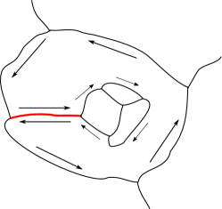
Figure 5: An example of an isthmus edge, shown in bold red. Arrows near edges denote the path for the left loop containing the isthmus.

Definition 2.

A left loop $(v_{1},\dots,v_{n},v_{n+1})$ is a left path where (i) $v_{1}=v_{n+1}$, (ii) $(v_{i-1},v_{i},v_{i+1})$ are distinct a left turns for $i=2,\dots,n$, and (iii) $(v_{n},v_{1},v_{2})$ is a left turn.

It is possible that both $(u,v)$ and $(v,u)$ are contained in a left loop. When this occurs, it follows that $(u,v)$ is an isthmus, or an edge whose removal disconnects the graph. See Fig. 5 for an example of an isthmus edge and its associated left loop. Since $\widetilde{G}$ is connected, a left loop uniquely determines a face, which we write as

$$f=[v_{1},\dots,v_{|f|}],$$ (4)

with the understanding that $(v_{1},\dots,v_{|f|},v_{1})$ is a left loop, and square brackets denote that (4) is an equivalence relation of left loops under a cyclic permutations of indices. The number of sides for a face is given by $|f|$. The collection $\Pi$ of left loops obtained from an embedding of a graph $G$ is known in combinatorial topology as a combinatorial embedding of $G$ [11]. As a convention, $\Pi$ does not include the left loop for the outer face obtained by traversing $\partial S$ clockwise. Note that $\Pi$ only consists of vertices in $G$, and contains no geometrical information from the embedding.

Definition 3.

The pair $\mathcal{G}=(G,\Pi)$ belongs to the space of combinatorial foams in $S$, denoted $\mathcal{C}(S)$, if $G$ is a simple trivalent connected graph and $\Pi$ is a combinatorial embedding of $G$ obtained from a simple foam.

In the language of computational geometry, combinatorial foams are provided through doubly-connected edge lists [9]. Loops can be recovered through repeatedly applying the next and previous pointers of half-edges (equivalent to direct edges).

2.2 Typical edges and rupturability

We now aim to identify edges in $\mathfrak{M}(S)$ whose ruptures are well-defined and follow the reaction (1). One implicit assumption in (1) is that an edge has four distinct neighboring cells: two for performing face merging and two others for edge merging. We formalize the differences between types of neighboring cells of an edge in the following definition.

Definition 4.

For an edge $e=\{u,v\}$ in $G$ and a combinatorial foam $\mathcal{G}=(G,\Pi)\in\mathcal{C}(S)$, a face $f\in\Pi$ is an edge neighbor of $e$ if $(u,v)$ or $(v,u)$ is in $f$. If there exist vertices $a,b\notin\{u,v\}$ such that $(a,u,b)$ or $(a,v,b)$ is a left turn in $f$, then $f$ is a vertex neighbor of $e$.

Edge and vertex neighbors will be those cells which will undergo face and edge merging in reaction (1), respectively. When considering common trivalent networks such as Archimedean lattices and almost every randomly generated Voronoi diagram, interior edges (those not intersecting $\partial S$) will have two edge neighbors and two vertex neighbors. This is in fact the maximum number of neighbors an edge can have.

Lemma 1.

For $\mathcal{G}=(G,\Pi)\in\mathcal{C}(S)$, then $e\in G$ can have at most four distinct neighbors. If $e$ has four neighbors, then two neighbors will be vertex neighbors, and two will be vertex neighbors.

Proof.

An edge $e=\{u_{0},v_{0}\}$ and its neighbors can be labeled as in Figure 6(a). The four left arcs

$$a_{1} =(u_{1},u_{0},v_{0},v_{1}), a_{2}=(v_{2},v_{0},u_{0},u_{2}),$$ (5)

$$a_{3} =(u_{2},u_{0},u_{1}), a_{4}=(v_{1},v_{0},v_{2})$$ (6)

contain all possible directed edges with $u_{0}$ or $v_{0}$ as an endpoint, which implies there can be at most four neighbors of $e$, in which case each arc belongs to a separate face. The two edge neighbors contain arcs $a_{1}$ and $a_{2}$, and the two vertex neighbors contain arcs $a_{3}$ and $a_{4}$. ∎

To limit reaction types, we will permit only edges with four neighbors to rupture, with the exception of boundary edges (those with vertices in $\partial S$) which have similar local configurations.

Definition 5.

An edge with four edge neighbors is a typical interior edge.

An edge $e$ is a typical boundary edge if either

(a) one and only one vertex of $e$ is in $\partial S$, and $e$ has two edge neighbors and one vertex neighbor, or

(b) both vertices of $e$ are in $\partial S$, and $e$ has two edge neighbors and no vertex neighbors.

The collection of typical interior edges and typical boundary edges are called typical edges.

There are multiple examples where an edge in $\widetilde{G}$ is atypical (not typical). For instance, an isthmus has only one edge neighbor. Other examples include neighbors of isthmuses. For each of these configurations, rupturing an atypical edge will produce reactions different from (1). See Appendix A for a cataloguing of atypical edges and their associated reactions.

A second issue arising in (1) occurs when a 3-gon is a reactant in edge merging, or two 3-gons are reactants in face merging, producing a 2-gon. However, 2-gons correspond to multiedges, and so are forbidden in simple foams. We impose one more requirement which ensures that all cells after rupture have at least three sides.

Definition 6.

A typical edge is rupturable if both of its vertex neighbors contain at least four edges, and at least one of its edge neighbors contains four edges. The set of rupturable edges for a combinatorial foam $\mathcal{G}$ is denoted $\mathcal{R}(\mathcal{G})$.

While we forbid 1- and 2-gons in simple foams for simplicity, we remark that they can exist in physical foams. Their behavior, however, can be quite erratic. For instance, when a 2-gon is formed, Burnett et al. [6] observed that sometimes the cell will slide along an edge until reaching a juncture, mutate into a 3-gon, and then quickly vanish to a point.

2.3 Edge rupture

We are now ready to define an edge rupture operation on $\mathcal{C}(S)$. For an interior rupturable edge $e=\{u_{0},v_{0}\}$, let $u_{i}$ and $v_{i}$ for $i=1,2$ denote the vertex neighbors for $u_{0}$ and $v_{0}$, labeled such that we have the left arcs (5)-(6) as shown in Figure 6(a). The four neighbors of $\{u_{0},v_{0}\}$ in $\Pi$ are written as

$$f_{1} =[u_{2},u_{0},u_{1},A_{1}],\qquad f_{2}=[v_{1},v_{0},v_{2},A_{3}],$$ (7)

$$f_{3} =[u_{1},u_{0},v_{0},v_{1},A_{2}]\qquad f_{4}=[v_{2},v_{0},u_{0},u_{2},A_{4}],$$ (8)

where $A_{1},\dots,A_{4}$ are left arcs. It is possible that $u_{i}=v_{j}$ for some $i,j\in\{1,2\}$ so that an edge neighbor is a 3-gon. However, $u_{1}\neq u_{2}$ and $v_{1}\neq v_{2}$ since this would make $G$ a multigraph. Also, the sets $\{u_{i}:i=1,2\}$ and $\{v_{i}:i=1,2\}$ are not equal, since this would force both edge neighbors of $e$ to have three sides, violating the rupturability conditions in Def. 6.

Definition 7.

For $\mathcal{G}=(G,\Pi)\in\mathcal{C}(S)$, we define an edge rupture $\Phi_{e}(\mathcal{G})$ for an edge $e=\{u_{0},v_{0}\}\in\mathcal{R}(\mathcal{G})$ through the mapping $(G,\Pi)\mapsto\mathcal{G}^{\prime}=(G^{\prime},\Pi^{\prime})$. If $G$ has vertices labeled as in Fig. 6(a), we obtain $G^{\prime}$ from $G$ by

1. Removing $\{u_{0},v_{0}\}$, followed by

2. Edge smoothing on the (now degree 2) vertices $u_{0}$ and $v_{0}$ by removing $\{u_{0},u_{1}\},\{u_{0},u_{2}\},\{v_{0},v_{1}\}$, and $\{v_{0},v_{2}\}$, and adding edges $\{u_{1},u_{2}\}$ and $\{v_{1},v_{2}\}$.

If $e$ is an interior edge, we obtain $\Pi^{\prime}$ by removing faces $f_{1},\dots,f_{4}$ from $\Pi$ and adding

$$f_{1}^{\prime}=[u_{2},u_{1},A_{1}],\quad f_{2}^{\prime}=[v_{2},v_{1},A_{3}],\quad f_{3}^{\prime}=[u_{1},u_{2},A_{4},v_{2},v_{1},A_{2}].$$ (9)

For a boundary edge where $u_{0}$ (or $v_{0}$) is in $\partial S$, the vertex neighbor $f_{1}$ (or $f_{2}$) does not exist, and we omit the addition of $f_{1}^{\prime}$ (or $f_{2}^{\prime}$) in (9).

A schematic of an embedding before and after edge rupture process is given in Fig. 6 (a)-(b). From counting sides of faces removed and added in rupture, we obtain

Lemma 2.

The types of reactions from edge rupture are limited to either

1. Interior rupture:

   $$C_{i}+C_{j}\rightharpoonup C_{i+j-4},\quad C_{k}\rightharpoonup C_{k-1},\quad C_{l}\rightharpoonup C_{l-1},$$ (10)

2. Boundary rupture with one vertex on $\partial S$:

   $$C_{i}+C_{j}\rightharpoonup C_{i+j-4},\quad C_{k}\rightharpoonup C_{k-1},$$ (11)

3. Boundary rupture with two vertices on $\partial S$:

   $$C_{i}+C_{j}\rightharpoonup C_{i+j-4}.$$ (12)

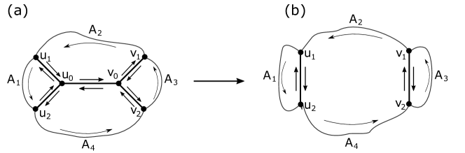
Figure 6: Left loops before and after the rupture of $\{u_{0},v_{0}\}$.

It is also straightforward to show

Lemma 3.

Let $\mathcal{G}=(G,\Pi)\in\mathcal{C}(S)$. If $e\in\mathcal{R}(\mathcal{G})$ and $\Phi_{e}(\mathcal{G})=(G^{\prime},\Pi^{\prime})$, then $G^{\prime}$ is connected.

Proof.

Since $e$ is rupturable, it cannot be an isthmus, so $G$ remains connected after removing $e$ in Step 1 of Def. 7. It is also connected after Step 2 as edge smoothing clearly maintains connectivity. ∎

Our main result is then

Theorem 1.

Edge rupture is closed in the space of combinatorial foams. In other words, for $\mathcal{G}=(G,\Pi)\in\mathcal{C}(S)$ and $e\in\mathcal{R}(\mathcal{G})$, then $\Phi_{e}(\mathcal{G})=(G^{\prime},\Pi^{\prime})\in\mathcal{C}(S)$.

Proof.

From Lemma 3, $G^{\prime}$ is connected and it is clear that Steps 1 and 2 in Def. 7 maintain trivalency. Furthermore, from the requirements for rupturable edges in Definition 6 and the possible reactions listed in Lemma 2, the three new faces in $G^{\prime}$ each have at least three sides. ∎

With Theorem 1, we are now ready to define a Markov chain for edge rupture in the state space $\mathcal{C}(S)$. For each state $\mathcal{G}\in\mathcal{C}(S)$, the range of possible one step transitions is given by $\cup_{e\in\mathcal{R}(\mathcal{G})}\Phi_{e}(\mathcal{G})$. If $|\mathcal{R}(\mathcal{G})|\geq 1$, we randomly select a rupturable edge uniformly, so that the probability transition kernel $p(\cdot,\cdot)$ is defined, for $e\in\mathcal{R}(\mathcal{G})$, by

$$p(\mathcal{G},\Phi_{e}(\mathcal{G}))=\frac{1}{|\mathcal{R}(\mathcal{G})|}.$$ (13)

In the case where there are no rupturable edges, we define $\mathcal{G}$ to be an absorbing state, so that $p(\mathcal{G},\mathcal{G})=1$. Uniform probabilities were also chosen for the simplest model of edge selection in [8] along with other distributions which considered geometric quantities such as the length of an edge. While we focus only on uniform selection of edges, more complicated transitions can be considered which depend on the local topological configurations of neighboring edges of $\mathcal{G}$.

Beginning with an initial state $\mathbf{G}(0)=\mathbf{G}_{0}\in\mathcal{C}(S)$, the Markov chain $\{\mathbf{G}(m)\}_{m\geq 0}$ is defined on $\mathcal{C}(S)$ recursively by obtaining $\mathbf{G}(m)$ from a random edge rupture on $\mathbf{G}(m-1)$. After generating an initial embedding and recording left loops to obtain an embedding topology $\mathbf{G}_{0}$, it is not necessary to use any geometrical quantities to perform one or more edge ruptures. If available, however, we may use vertex coordinates from initial conditions of a simple foam for providing a visual of sample paths. This is done by fixing positions of vertices, and adding new edges in Step 2 of Def. 7 as line segments. This method is especially convenient with initial conditions such as Voronoi diagrams and trivalent Archimedean lattices, which have straight segments as edges and vertex coordinates that are easy to numerically generate, store, and access. It should be noted that even with a valid combinatorial embedding, representing edges as line segments for each step may produce crossings in the visualization. However, in multiple simulations of networks we find that such crossings are exceedingly rare.

In Fig. 2 we show snapshots of a sample path $\{\mathbf{G}(m)\}_{0\leq m\leq 2000}$ under disordered initial conditions of a Voronoi diagram seeded with 2500 uniformly distributed initial site points in $S$. Fig. 3 is a sample path with ordered initial conditions of 2500 cells in a hexagonal lattice (an experimental method for generating two-dimensional physical foams with lattice and other ordered structures is outlined in [3]). In both figures, snapshots are taken after $250\cdot k$ ruptures for $k=0,\dots,8$. We observe that under both initial conditions, ruptures create networks which are markedly different from those obtained through mean curvature flow. The most evident distinction is in the creation of high-sided grains, which are bordered by a large number of 3 and 4-gons. Furthermore, the universal attractor of statistical topologies found from coarsening by gas diffusion [14, 20, 15, 19] does not appear in edge rupturing. We address statistical topologies in more detail in Section 5.

3 The mean-field model

In this section, we construct a simplified mean-field model of $\{\mathbf{G}(m)\}_{m\geq 0}$. The state space $E=\ell_{1}(\mathbb{N})$ consists of summable sequences $\mathbf{L}=(L_{3},L_{4},\dots)\in E$, with $L_{n}$ for $n\geq 3$ giving the total number of $n$-gons. For simplicity, our model consists of $n$-gons restricted to the single reaction (1). Since there is no notion of neighboring cells in $E$, we select four cells for face and edge merging randomly using only frequencies in $\mathbf{L}$. The mean-field rule is that for a randomly selected rupturable edge in a network, the probability that a vertex or edge neighbor is a $n$-gon is proportional to $n$, and that are no correlations between side numbers of the neighboring cells. Specifically, the mean-field probabilities we use for selecting a neighboring $n$-gon at state $\mathbf{L}$ are given by the two distributions

$$Q(n;\mathbf{L})=\frac{nL_{n}}{\sum_{i\geq 3}iL_{i}},\quad\widetilde{Q}(n;\mathbf{L})=\frac{nL_{n}\mathbf{1}_{n\geq 4}}{\sum_{i\geq 4}iL_{i}}.$$ (14)

Here, $Q$ is used for face merging, and allows for sampling among all cells, whereas $\widetilde{Q}$ forbids sampling 3-gons and is used for edge merging. Similar mean-field rules were a popular choice in the creation of minimal models for coarsening under gas diffusion [14, 20, 15]. It should be noted that nontrivial correlations exist for the number of sides in cells bordering the same edge. Studies for first and higher order correlations exist and depend on the type of network considered [1, 22]. Therefore, we should regard our selection probabilities $Q$ and $\widetilde{Q}$, which do not take these correlations into account, as estimates with errors that should not be expected to vanish as the number of cells becomes large.

We randomly select two cells for edge merging from $\mathbf{L}$, with the number of sides $\nu_{1}$ and $\nu_{2}$ obtained by sampling from $\widetilde{Q}$. Similarly, we select two cells for face merging, having $\sigma_{1}$ and $\sigma_{2}$ sides obtained by sampling from $Q$. After selecting these four cells, we update $\mathbf{L}$ in accordance with (1). This involves removing the four reactant cells having $\nu_{i}$ and $\sigma_{i}$ sides for $i=1,2$, and adding three product cells, having $\sigma_{1}+\sigma_{2}-4$, $\nu_{1}-1$, and $\nu_{2}-1$ sides.

In what follows, we state in detail the process of generating $\sigma_{i},\nu_{i}$ for $i=1,2$ through sampling from $\mathbf{L}$ without replacement. Steps (1)-(4) remove cells from $\mathbf{L}$ which are the reactants in (1), and step (5) adds the face and edge-merged products to create $\mathbf{L}^{\prime}$.

Mean-field process: For a state $\mathbf{L}\in E$ with $\sum_{i\geq 4}L_{i}\geq 3$ and $\sum_{i\geq 3}L_{i}\geq 4$, obtain the transitioned state $\mathbf{L}^{\prime}\in E$ through performing the following steps in order:

1. Sample $\nu_{1}\sim\widetilde{Q}(\cdot;\mathbf{L})$. Remove a $\nu_{1}$-gon from $\mathbf{L}$ and update remaining cells as $\mathbf{L}^{(1)}=(L^{(1)}_{3},L_{4}^{(1)},\dots)$, where $L^{(1)}_{\nu_{1}}=L_{\nu_{1}}-1$ and $L^{(1)}_{i}=L_{i}$ for $i\neq\nu_{1}$.

2. Sample $\nu_{2}\sim\widetilde{Q}(\cdot;\mathbf{L}^{(1)})$. Remove a $\nu_{2}$-gon from $\mathbf{L}^{(1)}$ and update remaining cells as $\mathbf{L}^{(2)}=(L^{(2)}_{3},L_{4}^{(2)},\dots)$, where $L^{(2)}_{\nu_{2}}=L_{\nu_{2}}^{(1)}-1$ and $L^{(2)}_{i}=L_{i}^{(1)}$ for $i\neq\nu_{2}$.

3. Sample $\sigma_{1}\sim Q(\cdot;\mathbf{L}^{(2)}).$ Remove a $\sigma_{1}$-gon from $\mathbf{L}^{(2)}$ and update remaining cells as $\mathbf{L}^{(3)}=(L^{(3)}_{3},L_{4}^{(3)},\dots)$, where $L^{(3)}_{\sigma_{1}}=L_{\sigma_{1}}^{(2)}-1$ and $L^{(3)}_{i}=L_{i}^{(2)}$ for $i\neq\sigma_{1}$.

4. Sample $\sigma_{2}\sim Q(\cdot;\mathbf{L}^{(3)}).$ If $(\sigma_{1},\sigma_{2})=(3,3)$, reject both $\sigma_{1}$ and $\sigma_{2}$ and repeat steps (3) and (4). If $(\sigma_{1},\sigma_{2})\neq(3,3)$, remove a $\sigma_{2}$-gon from $\mathbf{L}^{(3)}$ and update remaining cells as $\mathbf{L}^{(4)}=(L^{(4)}_{3},L_{4}^{(4)},\dots)$, where $L^{(4)}_{\sigma_{2}}=L_{\sigma_{2}}^{(3)}-1$ and $L^{(4)}_{i}=L_{i}^{(3)}$ for $i\neq\sigma_{2}$.

5. Add a $(\sigma_{1}+\sigma_{2}-4)$, $(\nu_{1}-1)$, and $(\nu_{2}-1)$-gon to $\mathbf{L}^{(4)}$ to obtain the transitioned state $\mathbf{L}^{\prime}=(L_{3}^{\prime},L_{4}^{\prime},\dots)$, with

   $$L_{n}^{\prime}= L_{n}^{(4)}+\mathbf{1}(\sigma_{1}+\sigma_{2}-4=n)+\sum_{j=1}^{2}\mathbf{1}(n=\nu_{j}-1).$$ (15)

Note that in Step 5 and in future equations we use the indicator notation for a statement $A$, written as either $\mathbf{1}(A)$ or $\mathbf{1}_{A}$, and defined as

$$\mathbf{1}(A)=\begin{cases}1&\hbox{if }A\hbox{ holds,}\\ 0&\hbox{otherwise.}\\ \end{cases}$$ (16)

The requirement that there are at least four cells, and that three cells have at least four sides is to ensure that sampling from $\widetilde{Q}$ and $Q$ is always possible. Note that the sampling algorithm accounts for the edge rupture conditions in Def. 6 by restricting sampling to occur with on cells with at least four sides in Steps 1 and 2, and also by the rejection condition in Step 4 forbidding both cells for face merging to be 3-gons. To ensure the sampling process is well-defined, we define states with $\sum_{i\geq 4}L_{i}<3$ or $\sum_{i\geq 3}L_{i}<4$ as absorbing so that $\mathbf{L}^{\prime}=\mathbf{L}$.

If we consider an initial distribution of cells $\mathbf{L}(0)\in E$, by the above process we may obtain a Markov chain $\{\mathbf{L}(m)\}_{m\geq 0}$ defined on $E$ by through the recursive formula $\mathbf{L}(m)=(\mathbf{L}(m-1))^{\prime}$. Like $\{\mathbf{G}(m)\}_{m\geq 0}$, it is evident that at each nonabsorbing state the total number of cells decreases by one, and sum of edges over all cells decreases by six. In other words, under norms $\|\mathbf{L}\|=\sum_{i\geq 3}L_{i}$ and $\|\mathbf{L}\|_{s}=\sum_{i\geq 3}iL_{i}$,

$$\|\mathbf{L}(m)\|=\|\mathbf{L}(m-1)\|-1,\quad\hbox{}\quad\|\mathbf{L}(m)\|_{s}=\|\mathbf{L}(m-1)\|_{s}-6.$$ (17)

We compare statistics of $n$-gons between the mean-field and network model in Section 5.

4 Kinetic equations of the mean-field model

By considering a network with large number of cells, we give a derivation of a hydrodynamic limit for the state transition given in the previous section. For the mean-field process $\mathbf{L}^{N}(m)$ with $N$ initial cells, we define time increments $t_{m}^{N}=m/N$ to write the number densities of $n$-gons as a continuous time càdlàg jump process

$$u_{n}^{N}(t;\gamma)=\sum_{m\geq 0}\frac{L_{n}^{N}(m)}{N}\cdot\mathbf{1}(t\in[t_{m}^{N}/\gamma,t_{m+1}^{N}/\gamma)),\quad t\geq 0.$$ (18)

Here we have included a constant parameter $\gamma>0$ denoting the rate of edge ruptures per unit time. Under the existence of limiting number densities $u_{n}^{N}(t)\rightarrow u_{n}(t)$ as $N\rightarrow\infty$, we formally derive limiting kinetic equations by computing limiting probabilities (14) of cell selection probabilities in face and edge merging.

In the kinetic limit, the $n$-gon growth rate $\dot{u}_{n}$ is equal to the edge rupture rate $\gamma$ multiplied by the expected number $H_{n}[u]$ of $n$-gons gained at a rupture with limiting number densities $u=(u_{3},u_{4},\dots)$. Decomposing $H_{n}[u]$ with respect to different reactions, we obtain the infinite system

$$\dot{u}_{n}=\gamma(H_{n,+}^{F}[u]+H_{n,+}^{E}[u]-H_{n,-}^{F}[u]-H_{n,-}^{E}[u]),\quad n\geq 3,$$ (19)

where $H_{n,\pm}^{F/E}$ denote the expected number of created $(+)$ and annihilated $(-)$ $n$-gons from face ($F$) and edge $(E)$ merging. In what follows, we compute the explicit formulas for each term in (19).

As $N\rightarrow\infty$, the differences in probabilities in the mean-field sampling process for sampling without replacement vanish, so that limiting probabilities in steps (1)-(4) of the mean-field sampling process for selecting reactants can be given solely in terms of $u$. The limiting distribution of $Q$ in (14) is given by

$$p_{n}=\frac{nu_{n}}{S(u)},\quad S(u)=\sum_{k\geq 3}ku_{k},$$ (20)

and the limiting distribution of $\widetilde{Q}$ is

$$\widetilde{p}_{n}=\frac{nu_{n}}{\widetilde{S}(u)}\mathbf{1}_{n\geq 4},\quad\widetilde{S}(u)=\sum_{k\geq 4}ku_{k}.$$ (21)

From the reaction $C_{n+1}\rightharpoonup C_{n}$, we write the expected number of created $n$-gons from edge merging as

$$H_{n,+}^{E}=2\widetilde{p}_{n+1}=2q_{n+1}^{E}u_{n+1},\quad q_{n}^{E}:=\frac{n\mathbf{1}_{n\geq 4}}{\widetilde{S}}.$$ (22)

The factor of two in (22) accounts for the two edge merging reactions involved in each rupture. From the reaction $C_{n}\rightharpoonup C_{n-1}$, the expected number of annihilated $n$-gons from edge merging is then

$$H_{n,-}^{E}=2\widetilde{p}_{n}=2q_{n}^{E}u_{n}.$$ (23)

Computing expected $n$-gons from face merging involves a straightforward conditional probability calculation. Let $\Sigma_{1}$ and $\Sigma_{2}$ be iid random variables with $\mathbb{P}(\Sigma_{1}=n)=p_{n}$ for $n\geq 3$. Then the number of sides $(\sigma_{1},\sigma_{2})$ for the two cells selected for face merging has the same law as $(\Sigma_{1},\Sigma_{2})$ under the edge rupture condition that $(\Sigma_{1},\Sigma_{2})\neq(3,3)$. The expected number of $n$-gons selected under the reaction $C_{i}+C_{j}\rightharpoonup C_{i+j-4}$ is then computed with linearity of expectation and the definition of conditional probability:

$$H_{n,-}^{F}=\mathbb{E}[\mathbf{1}_{\sigma_{1}=n}+\mathbf{1}_{\sigma_{2}=n}] =\mathbb{E}[\mathbf{1}_{\Sigma_{1}=n}+\mathbf{1}_{\Sigma_{2}=n}|(\Sigma_{1},\Sigma_{2})\neq(3,3)]$$ (24)

$$=\frac{2p_{3}}{1+p_{3}}\mathbf{1}_{n=3}+\frac{2p_{n}}{1-p_{3}^{2}}\mathbf{1}_{n\geq 4}.$$ (25)

This may also be written as

$$H_{n,-}^{F}=2q_{n}^{F}u_{n},\quad q_{n}^{F}:=\frac{3}{S(1+p_{3})}\mathbf{1}_{n=3}+\frac{n}{S(1-p_{3}^{2})}\mathbf{1}_{n\geq 4}.$$ (26)

Here, the factor of two comes from the two reactants in the single reaction for cell merging in (1).

A similar calculation gives the probability for a pairing of cells in face merging, with

$$p_{i,j}:=\mathbb{P}((\sigma_{1},\sigma_{2})=(i,j))=\frac{p_{i}p_{j}}{1-p_{3}^{2}},\quad(i,j)\neq(3,3).$$ (27)

The creation of $n$-gons through face merging can be enumerated by reactions $C_{i}+C_{4+n-i}\rightharpoonup C_{n}$ for $i=3,\dots,n+1$. The expected number of $n$-gons created is then

$$K^{F}_{i,j} :=\frac{ij\mathbf{1}(i,j\geq 3,(i,j)\neq(3,3))}{S^{2}(1-p_{3}^{2})},$$ (28)

$$H_{n,+}^{F} =\sum_{i=3}^{n+1}p_{4+n-i,i}=\sum_{i=3}^{n+1}K^{F}_{4+n-i,i}u_{4+n-i}u_{i}.$$ (29)

From (20)-(28), we can express $H_{n}$ explicitly in terms of $p_{k}$ and $\widetilde{p}_{k}$. For $3\leq n\leq 6$,

$$H_{3} =\frac{2p_{3}p_{4}}{1-p_{3}^{2}}-\frac{2p_{3}}{1+p_{3}}+2\widetilde{p}_{4},$$ (30)

$$H_{4} =\frac{p_{4}^{2}+2(p_{3}p_{5}-p_{4})}{1-p_{3}^{2}}+2(\widetilde{p}_{5}-\widetilde{p}_{4}),$$ (31)

$$H_{5} =\frac{2(p_{3}p_{6}+p_{4}p_{5}-p_{5})}{1-p_{3}^{2}}+2(\widetilde{p}_{6}-\widetilde{p}_{5}),$$ (32)

$$H_{6} =\frac{2(p_{3}p_{7}+p_{4}p_{6}-p_{6})+p_{5}^{2}}{1-p_{3}^{2}}+2(\widetilde{p}_{7}-\widetilde{p}_{6}).$$ (33)

Combining (22), (26), and (28), we rewrite (19) as an infinite-dimensional system of nonlinear, autonomous ordinary differential equations to obtain

$$\dot{u}_{n} =\gamma\cdot\left(\sum_{i=3}^{n+1}K^{F}_{4+n-i,i}u_{4+n-i}u_{i}+2q_{n+1}^{E}u_{n+1}-2q_{n}^{F}u_{n}-2q_{n}^{E}u_{n}\right)$$ (34)

for $n\geq 3$.

We note a subtlety with regards to face merging and 4-gons, due to the merging of an $n$-gon and a 4-gon producing another $n$-gon. This reaction means that face merging of an $n$-gon with a $4$-gon does not result in the annihilation of an $n$-gon. Therefore, if we substitute $p_{n}=(1-p_{3}^{2})\sum_{i\geq 3}p_{n,i}$ into the numerators of (25), terms containing $p_{n,4}$, corresponding to the reaction $C_{n}+C_{4}\rightharpoonup C_{n}$, should not be included in $H_{-}^{F}$. On the other hand, these same probabilities appear equally in $H_{+}^{F}$, corresponding to $i=4$ and $n$ for the sum in (29), in which the merging of a $n$-gon and 4-gon does not increase the total number of $n$-gons. Thus the total contribution of $n$-gons by face merging with $4$-gons in (34) is zero, and equation (34) still holds.

Setting $\gamma\ =1$ and summing (34) over $n\geq 3$, we find formal growth rates for the zeroth and first moments of $u$, with

$$\sum_{n\geq 3}\dot{u}_{n}=\sum_{n\geq 3}H_{n}[u]=-1\quad\hbox{ and }\quad\sum_{n\geq 3}n\dot{u}_{n}=\sum_{n\geq 3}nH_{n}[u]=-6.$$ (35)

This simply reflects the fact that each rupture reduces the number of cells in the foam by one and reduces the number of sides by six. Since the dynamical system is infinite dimensional, however, it is not necessarily true that we can interchange the derivative and sum in (35) and deduce that the total side number $S(u)=\sum_{k\geq 3}ku_{k}$ satisfies $\dot{S}=-6$. A similar issue arises in other models of coagulation with sufficiently fast collision rates, in which conservation of the first moment, or mass, exists until some nonnegative time $T_{\mathrm{gel}}$ at which total mass starts to decrease. A popular example is the Smoluchowski equation [24] for coalescing clusters $A_{n}$ of size $n$ under the second order reaction

$$A_{i}+A_{j}\rightharpoonup A_{i+j}.$$ (36)

The proportion $v_{n}$ of size $n$ clusters is given by

$$\dot{v}_{n}=\frac{1}{2}\sum_{j=1}^{n-1}K_{n-j,j}v_{n-j}v_{j}-\sum_{j\geq 1}K_{n,j}v_{n}v_{j},\quad n\geq 1$$ (37)

for a collision kernel $K$ describing rates of cluster collisions. The kernel $K^{F}$ for cell merging in (28) bears resemblance to the multiplicative kernel $K_{i,j}=ij$ for (37), differing by a factor depending on $S$ and $p_{3}$. For (37) with the multiplicative kernel, it is well known that a gelation time $T_{\mathrm{gel}}$ exists, meaning that the total mass $\sum_{k\geq 1}kv_{k}(t)$ is conserved for $t\leq T_{\mathrm{gel}}$, and then decreases for $t>T_{\mathrm{gel}}$ [21]. The interpretation is that while the total mass of finite size clusters decreases, the remaining total mass is contained in an infinite sized cluster called a gel.

An equivalent definition of gelation time for the Smoluchowski equations comes from a moment analysis (see [2] for a thorough summary). Denote the $k$th moment for solutions of (37) as $m_{k}^{S}(t)=\sum_{j\geq 1}j^{k}v_{j}(t)$. The gelation time $T_{\mathrm{gel}}$ is then defined as the (possibly infinite) blowup time of $m_{2}^{S}(t)$. A finite gelation time implies an explosive flux of mass toward a large cluster, and occurs when $m_{1}^{S}(t)$ begins to decrease. To see the blowup of $m_{2}^{S}$, we compare the squared cluster sizes of products and reactants in (36), with

$$|A_{i+j}|^{2}-|A_{i}|^{2}-|A_{j}|^{2}=2ij.$$ (38)

The rate of growth for the second moment is found by summing, over $i$ and $j,$ the difference of squares in (38) multiplied by the expected number of collisions $v_{i}v_{j}K(i,j)/2$. Thus,

$$\dot{m}_{2}^{S}=\sum_{i,j\geq 1}ijK(i,j)v_{i}v_{j}.$$ (39)

Under the multiplicative kernel $K(i,j)=ij$, (39) with monodisperse initial conditions ($v_{1}(0)=1$ and $v_{j}(0)=0$ for $j\geq 2$) reduces to the elegant form

$$\dot{m}_{2}^{S}=(m_{2}^{S})^{2}\quad\Rightarrow\quad m_{2}^{S}(t)=(1-t)^{-1},\quad t\in[0,1).$$ (40)

To compare with our kinetic equations for foams with edge rupture, we denote moments as $m_{k}(t)=\sum_{j\geq 3}j^{k}u_{j}(t)$. The difference of squares from side numbers before and after reaction (1) is given by

$$|C_{i+j-4}|^{2}-|C_{i}|^{2}-|C_{j}|^{2}=2ij-8(i+j)+16$$ (41)

for face merging and two instances of

$$|C_{k-1}|^{2}-|C_{k}|^{2}=-2k+1$$ (42)

for edge merging. Ignoring technical issues of interchanging infinite sums, we formally compute that the second moment grows as

$$\dot{m}_{2} =\sum_{\begin{subarray}{c}i,j\geq 3\\ (i,j)\neq(3,3)\end{subarray}}(2ij-8(i+j)+16)K^{F}(i,j)u_{i}u_{j}+2\sum_{k\geq 4}(-2k+1)q^{E}_{k}u_{k}$$ (43)

$$=\frac{2m_{2}^{2}-16m_{1}m_{2}+16m_{1}^{2}-126u_{3}^{2}}{m_{1}^{2}(1-p_{3}^{2})}-\frac{4m_{2}-2m_{1}-30u_{3}}{m_{1}-3u_{3}}.$$ (44)

As the quadratic term $m_{2}^{2}$ in (44) is similar to (39), we conjecture a finite-time blowup of $m_{2}$. However, we will withhold a more rigorous moment analysis for future work, and note that the time dependent first moment $m_{1}(t)$ and proportion of 3-gons $u_{3}(t)$ will almost certainly present difficulties in either solving or estimating $m_{2}$. In particular, it is possible that $3u_{3}$ may approach $m_{1}$ in finite time, creating a singularity in (44).

5 Numerical experiments

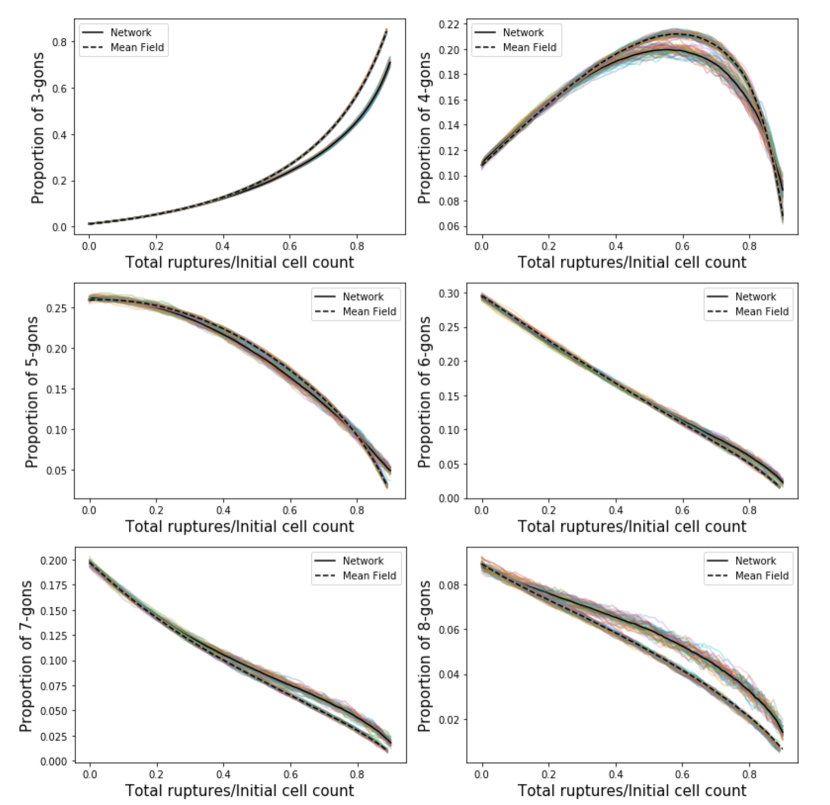
Figure 7: Fractions of total ruptures over initial cell count and number densities of $n$-gons for network and mean-field models under disordered initial conditions with $n=3,\dots,8$. Samples paths are plotted with transparency and mean paths are plotted with solid (network) and dashed (mean-field) lines.

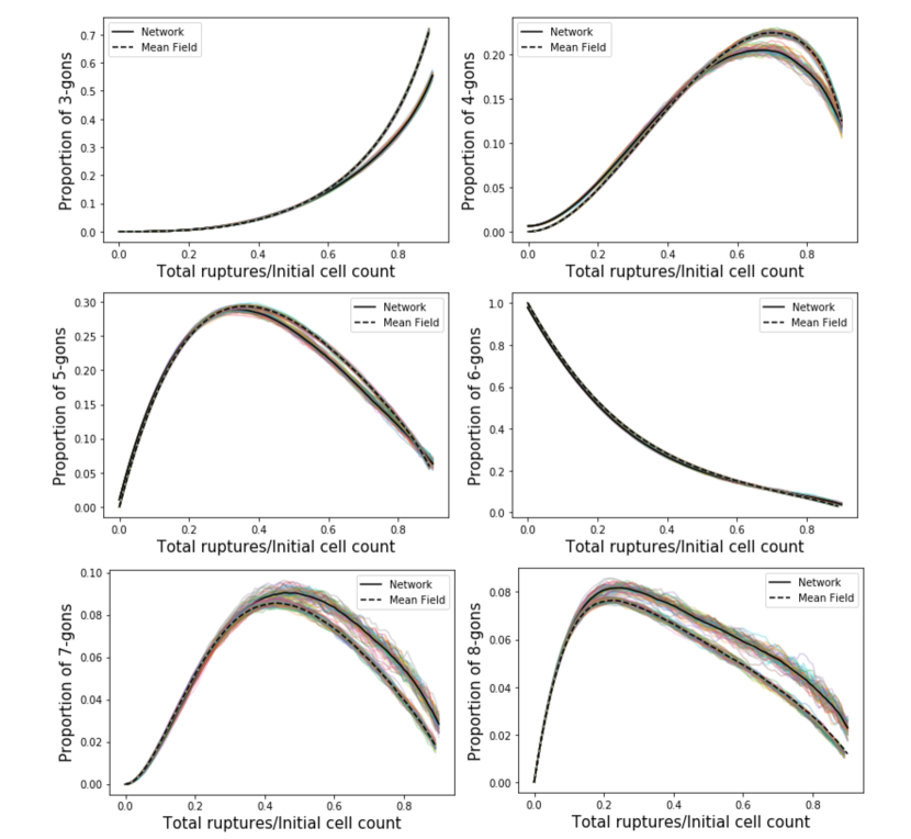
Figure 8: Fractions of total ruptures over initial cell count and number densities of $n$-gons for network and mean-field models under ordered initial conditions with $n=3,\dots,8$. Samples paths are plotted with transparency and mean paths are plotted with solid (network) and dashed (mean-field) lines.

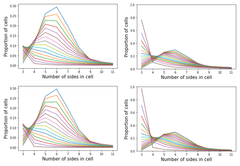
Figure 9: Statistical topologies for disordered initial conditions for fractions $.06k$ for $k=0,\dots,15$ of total ruptures over the initial number of cells. Solid lines between integers are for ease in visualization. As a guide, in all figures, fractions for $6$-gons are largest at time 0 and decrease as ruptures increase. Top: Subprobabilities (left) and probabilities (right) for network model. Bottom: Subprobabilities (left) and probabilities (right) for mean-field model.

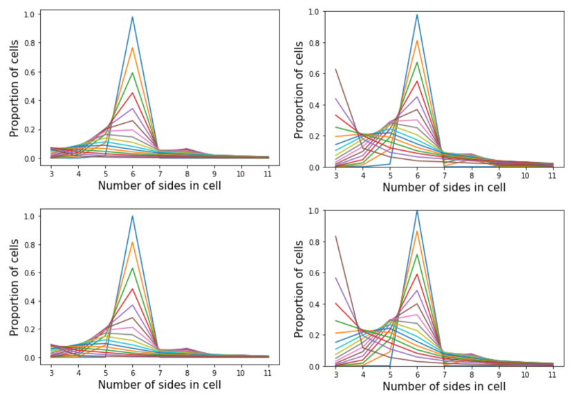
Figure 10: Statistical topologies for ordered initial conditions for fractions $.06k$ for $k=0,\dots,15$ of total ruptures over the initial number of cells. Solid lines between integers are for ease in visualization. As a guide, in all figures, fractions for $6$-gons are largest at time 0 and decrease as ruptures increase. Top: Subprobabilities (left) and probabilities (right) for network model. Bottom: Subprobabilities (left) and probabilities (right) for mean-field model.

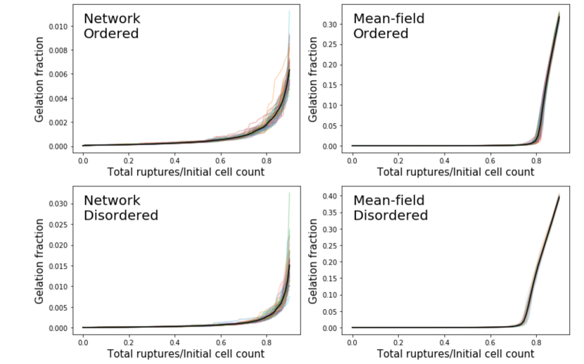
Figure 11: Fractions of total ruptures over initial cell count and gelation fractions. Top: Ordered initial conditions for network (left) and mean-field (right) models. Bottom: Disordered initial conditions for network (left) and mean-field (right) models. Samples paths are plotted with transparency and mean paths are plotted with solid lines.

In this section, we compare simulations between the Markov chains $\{\mathbf{G}(m)\}_{m\geq 0}$ and $\{\mathbf{L}(m)\}_{m\geq 0}$. For simulating the network model, we consider disordered initial conditions of a Voronoi diagram with a uniform random seeding of $3\times 10^{4}$ site points, and also ordered initial conditions of a hexagonal (honeycomb) lattice. For each of these initial conditions, we implement the voronoi library in Python to provide the initial combinatorial embedding through a doubly connected edge list, from which we randomly sample rupturable edges. Over 50 simulations, we decrease the number of cells by a decade, performing $2.7\times 10^{4}$ ruptures. For the mean-field model, we compute the initial distribution of $n$-gons by generating Voronoi diagrams, and for ordered hexagonal lattice conditions we set all cells to have six sides. For 50 simulations, we perform simulations with $10^{5}$ initial cells and $9\times 10^{4}$ ruptures. Both experiments take approximately 20 minutes to perform, although the mean-field model is substantially easier to implement. Attempting to increase the initial number of cells in the network model to $10^{5}$ greatly increased the run time. As we shall we, however, using $3\times 10^{4}$ initial cells was sufficient in creating approximately deterministic statistics for comparing against the mean-field model.

A plot comparing total ruptures and number densities of $n$-gons is given in Figs. 7 and 8. A time scale is given by the total number of ruptures over the initial number of cells, which corresponds to the time scale in (19) with $\gamma=1$. Each sample path is plotted with transparency along with the mean path of the samples. We observe in both models that the evolution of $n$-gons appears to approach a deterministic limit, although we observe greater variance in sample paths for 7 and 8-gons. This is due to relatively fewer cells having 7 or 8 sides, especially as the foam ages. For disordered initial conditions, number densities of $n$-gons decrease for $n\geq 5$. The number density of 4-gons reach a local maximum when about half as many cells remain, while 3-gons increase during the entire process. When 10% of cells remain, approximately 70% of cells in the network model and nearly 90% in the mean-field model are 3-gons. This difference gives the greatest discrepancies between the two models. For comparing other $n$-gons, number densities agree to within a few percentage points, with particularly accurate behavior during the first half of the process. The two models also agree especially well for 6-gons during the entire simulation. Similar behavior occurs with ordered initial conditions, although number densities for 4, 5, 7, and 8-gons experience a temporary increase as the network mutates from initially monodisperse conditions of 6-gons.

The evolution of statistical topologies is given in Figs. 9 and 10. To keep the graphs readable, we plot only the mean frequencies over the 50 simulations, but Figs. 7 and 8 show that the variations between mean and pathwise frequencies are small. We note that number densities in (18) are actually subprobabilities, since in (18) we are scaling the total number of $n$-gons at all times against the initial number of cells $N$. We also consider normalized number densities $\hat{u}_{n}^{N}=u_{n}^{N}/\sum_{j\geq 3}u_{j}^{N}$, shown in Figures 9 and 10. Such a normalization more clearly demonstrates the differences of frequencies between low-sided grains.

The most interesting difference between the two models occurs when comparing cells having the most sides. We define the gel fraction of a combinatorial foam $\mathcal{G}=(G,F)$ and a state $\mathbf{L}\in E$ by

$$\mathrm{Gel}(\mathcal{G})=\frac{\max\{|f|:f\in F\}}{\sum_{f\in F}|f|},\quad\mathrm{Gel}(\mathbf{L})=\frac{\max\{i:L_{i}>0\}}{\|\mathbf{L}\|_{s}}.$$ (45)

In words, the gel fraction is the largest fraction of total sides from a single cell. For ordered initial conditions, we observe in Fig. 11 that gelation occurs at about $T_{\mathrm{gel}}=.8$, meaning that $\mathrm{Gel}(\mathbf{L})$ is approximately zero until $T_{\mathrm{gel}}$, and suddenly increases past this point. For disordered intial conditions, gelation occurs at approximately $T_{\mathrm{gel}}=.75$. Past the gelation time, the gelation fraction appears to grow at a roughly linear rate until the process is terminated at $t=.9.$ Gel fractions in the network model, however, are quite negligible, with sample paths having $\mathrm{Gel}(\mathcal{G})$ rarely above .02, and not having the ‘elbow’ found in the mean-field model marking a sudden increase in gel fraction. We conjecture the lack of gelation is likely due to the edge rupture conditions in Def. 6. While such conditions allow for deriving a simple mean-field model and limiting kinetic equations, aged foams in the network model produce a large amount of 3-gons which forbid neighboring edges to rupture and merge large adjacent cells.

6 Conclusion

We have studied a minimal Markov chain on the state space of combinatorial embeddings which models the rupture of edges in foams. The model can be further simplified by a mean-field assumption on the selection of which cells are neighbors of a rupturing edge, producing a Markov chain on the state space $\ell_{1}(\mathbb{N})$. An advantage to using such a mean-field model is in the derivation of limiting kinetic equations (34), a nonlinear infinite system which bears resemblance to the Smoluchowski coagulation equations with multiplicative kernel. Numerical simulations of the mean-field show a similar phase transition (the creation of a gel) also seen in models of coagulation. A quadratic term in the formal derivation of the first order ODE (43)-(44) suggests that the second moment $m_{2}(t)$ has finite time blowup, but it remains to show this rigorously.

A number of computational and mathematical questions can be raised from this study. First, it should be noted that the kinetic equations (34) do not account for interactions between cells with finitely many sides and the hypothesized gel (an $\infty$-gon). Thus, our kinetic equations are only valid in the pre-gelation phase. Since we should expect the $\infty$-gon to interact with the rest of the foam after gelation, the kinetic equations should be augmented, akin to the Flory model of polymer growth [13], to include a term $u_{\infty}(t)$ for the fraction of sides belonging to the gel. A numerical investigation relating the mean-field process to a discretization scheme of the kinetic equation, perhaps similar to the finite-volume method used in [12], would prove useful in estimating gelation times as well as convergence rates of the stochastic mean-field process to its law of large numbers limit.

We may also focus on the more combinatorial related questions of the network model. One hypothesis is that more significant gelation behavior will arise under relaxed conditions for rupture. While dropping rupturability conditions offers a more realistic version of edge rupture, cataloguing possible reactions becomes much more complicated, as outlined in Appendix A. Advances in proving a phase transition for the network model could potentially use methods from the similar problem of graph percolation [5]. Here, edges are randomly occupied in a large graph, and a phase transition corresponds when the probability of edge selection passes a percolation threshold to create a unique graph component of occupied edges. Bond percolation thresholds have been established in a variety of networks, including hexagonal lattices [25] and Voronoi diagrams [4].

Finally, we mention a natural way for introducing cell areas. While we have interpreted networks as foams, we can alternatively see them as spring networks, with vertices as point masses and edges as springs between the points. This allows a natural interpretation of areas arising from Tutte’s spring theorem [26], which creates a planar network as minimizing distortion energy of the spring network, and cell areas can easily be computed once the minimal configuration is found through solving a linear system. A random ‘snipping’ of springs would typically produce the same topological reaction (1), but with spring embedding we may now ask questions regarding gelation for both topology and area.

Acknowledgements: The author wishes to thank Anthony Kearsley and Paul Patrone for providing guidance during his time as a National Research Council Postdoctoral Fellow at the National Institute of Standards and Technology, and also Govind Menon for helpful suggestions regarding the preparation of this paper.

Appendix A Typical and atypical reactions

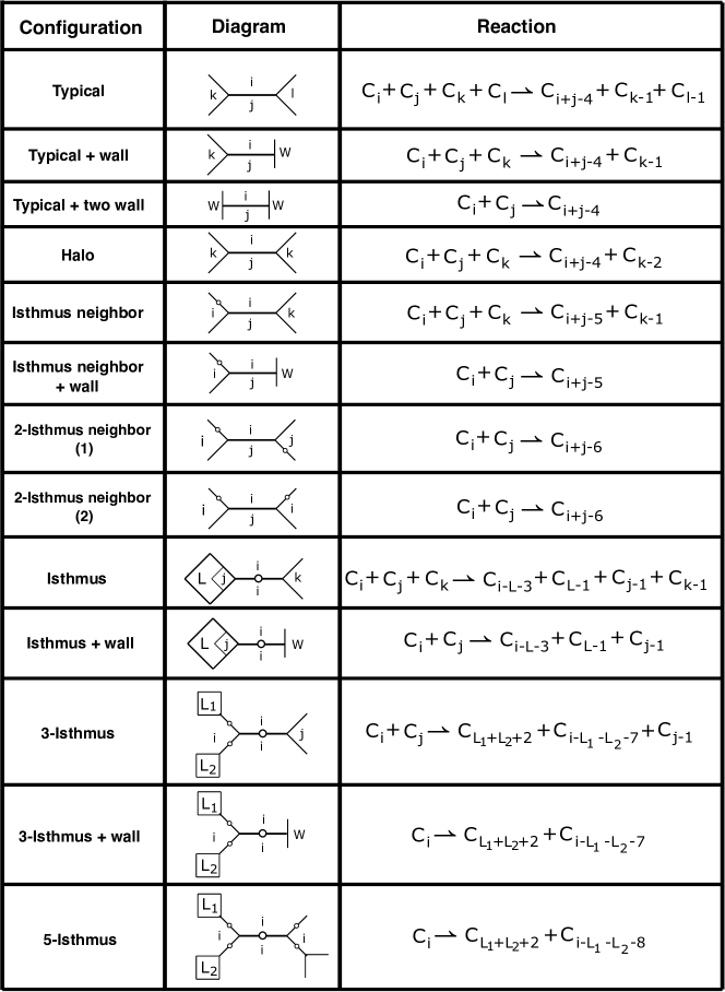
Figure 12: Typical and atypical reactions. The rupturable edge in each diagram is the horizontal edge in the center of the diagram. An edge with a $\circ$ symbol in its center denotes an isthmus. A vertical edge with $W$ denotes that a vertex of the rupturable edge is contained on a wall. For the 3-isthmus, 3-isthmus+wall, and 5-isthmus, a square with $L_{i}$ for $i=1,2$ denotes a left arc connected to an isthmus with $L_{i}$ sides. For isthmus and isthmus+wall, the square with $j$ denotes a $j$-gon connected to an isthmus, and the square with $L$ denotes a left arc containing $L$ sides (including the two contained in the $k$-gon and connected to the isthmus).

By removing the condition in Def. 6 that a rupturing edge must be typical, we can consider the broader collection of atypical configurations and their corresponding reactions. A diagram of the thirteen different local configurations and the twelve different reactions for typical and atypical edges are given in Fig. 12. For some of these reactions, there are cells which undergo both edge and face merging, so for simplicity the collection of reacting cells and their products are listed as a single reaction. For each reaction listed, we assume a sufficient number of sides in each reactant cell so that all products have at least three sides. The set of atypical edges includes isthmuses, whose rupture disconnects the foam. If we wished to continue rupturing after rupturing an isthmus, it would be necessary to relax the requirement of connectivity in a simple foam, which in turn would further increase possible reactions. Even more reactions are possible by permitting foams to include loops (1-gons) and multiedges (2-gons). For now, we withhold from enumerating this rather complicated set of reactions.

We now give an informal derivation for how the enumeration in Fig. 12 is obtained. This is done by counting reactions in configurations arising from whether a rupturable edge $e=\{u_{0},v_{0}\}$ or its neighbors are isthmuses. We begin by considering configurations with no isthmuses. We have already discussed the three typical reactions (10)-(12). There is also the possibility that an interior edge $e$ contains two edge neighbors and a single vertex neighbor containing both $u_{0}$ and $v_{0}$. This cell wraps around several other cells to contain both vertices, so we call such a configuration a halo.

If $e$ is not an isthmus, it is possible for either one or two incident edges to be isthmuses, but no more. This follows from the fact that if two isthmuses are incident to a vertex, then the third incident edge must be an isthmus as well. This creates four possible configurations: two containing one isthmus neighbor with or without a vertex contained on the boundary, and another containing two isthmus neighbors (both of which producing the same reaction $C_{i}+C_{j}\rightharpoonup C_{i+j-6})$. Since the original edge is not an isthmus, each of these configurations after rupture remains connected.

We finally consider the set of configurations for when $e$ is an isthmus. If no other edges are isthmuses, then $e$ can be in the interior of $S$ or have a single vertex in $\partial S$ (two such vertices on $\partial S$ would imply that $e$ is not an isthmus). One or both of $u_{0}$ or $v_{0}$ can have all of its incident edges as isthmuses. If one vertex of $e$ has three incident isthmuses, then the other vertex can either be on $\partial S$, or have one or three incident isthmuses. In total, there are five different reactions with $e$ as an isthmus.

Some care is needed when counting the products for reactions with isthmuses. Under the left path interpretation for face sides, isthmuses count for two sides. Additionally, the rupture of an isthmus will disconnect the network. This results in the creation of a new ‘island’ cell with a left path of exterior edges around the island, which are also removed from the cell originally contained ruptured isthmus $e$. In all reactions, the change in total number of sides is given by the number of boundary vertices in $e$ minus six.

In each atypical reaction, the process of edge removal and insertion is indeed the same as typical reactions. Updates for left loops in the combinatorial foam are more complicated, and will depend on the local configuration. As an example, let us consider the isthmus neighbor configuration, which has a single vertex neighbor $f_{1}$ and two edge neighbors $f_{2},f_{3}$. We write the left loops of these neighbors as

$$f_{1}=[v_{1},v_{0},v_{2},A_{2}],\qquad f_{2}=[v_{2},v_{0},u_{0},u_{2},A_{1}],$$ (46)

$$f_{3}=[u_{1},u_{0},v_{0},v_{1},A_{3},u_{2},u_{0},u_{1},A_{4}],$$ (47)

where $\{u_{0},u_{1}\}$ is an isthmus, and $A_{1},\dots,A_{4}$ are left arcs. After rupture, there are two cells remaining, with left loops

$$f_{2}^{\prime}=[v_{1},v_{2},A_{2}],\quad f_{2,3}^{\prime}=[u_{1},u_{2},A_{1},v_{2},v_{1},A_{3},u_{2},u_{1},A_{4}].$$ (48)

Conflict of interest

The author declares that he has no conflict of interest.

References

- [1] D. Aboav, The arrangement of grains in a polycrystal, Metallography, 3 (1970), pp. 383–390.
- [2] D. J. Aldous et al., Deterministic and stochastic models for coalescence (aggregation and coagulation): a review of the mean-field theory for probabilists, Bernoulli, 5 (1999), pp. 3–48.
- [3] J. Bae, K. Lee, S. Seo, J. G. Park, Q. Zhou, and T. Kim, Controlled open-cell two-dimensional liquid foam generation for micro-and nanoscale patterning of materials, Nature communications, 10 (2019), pp. 1–9.
- [4] A. M. Becker and R. M. Ziff, Percolation thresholds on two-dimensional voronoi networks and delaunay triangulations, Physical Review E, 80 (2009), p. 041101.
- [5] B. Bollobás, B. Bollobás, O. Riordan, and O. Riordan, Percolation, Cambridge University Press, 2006.
- [6] G. Burnett, J. Chae, W. Tam, R. M. De Almeida, and M. Tabor, Structure and dynamics of breaking foams, Physical Review E, 51 (1995), p. 5788.
- [7] I. Cantat, S. Cohen-Addad, F. Elias, F. Graner, R. Höhler, O. Pitois, F. Rouyer, and A. Saint-Jalmes, Foams: structure and dynamics, OUP Oxford, 2013.
- [8] J. Chae and M. Tabor, Dynamics of foams with and without wall rupture, Physical Review E, 55 (1997), p. 598.
- [9] M. De Berg, M. Van Kreveld, M. Overmars, and O. Schwarzkopf, Computational geometry, in Computational geometry, Springer, 1997, pp. 1–17.
- [10] J. Duplat, B. Bossa, and E. Villermaux, On two-dimensional foam ageing, Journal of fluid mechanics, 673 (2011), pp. 147–179.
- [11] J. R. Edmonds Jr, A combinatorial representation for oriented polyhedral surfaces, PhD thesis, 1960.
- [12] F. Filbet and P. Laurençot, Numerical simulation of the smoluchowski coagulation equation, SIAM Journal on Scientific Computing, 25 (2004), pp. 2004–2028.
- [13] P. J. Flory, Molecular size distribution in three dimensional polymers. i. gelation1, Journal of the American Chemical Society, 63 (1941), pp. 3083–3090.
- [14] H. Flyvbjerg, Model for coarsening froths and foams, Physical Review E, 47 (1993), p. 4037.
- [15] V. Fradkov, A theoretical investigation of two-dimensional grain growth in the ‘gas’ approximation, Philosophical Magazine Letters, 58 (1988), pp. 271–275.
- [16] J. A. Glazier, S. P. Gross, and J. Stavans, Dynamics of two-dimensional soap froths, Physical Review A, 36 (1987), p. 306.
- [17] J. A. Glazier and D. Weaire, The kinetics of cellular patterns, Journal of Physics: Condensed Matter, 4 (1992), p. 1867.
- [18] C. Herring, Surface tension as a motivation for sintering, in Fundamental Contributions to the Continuum Theory of Evolving Phase Interfaces in Solids, Springer, 1999, pp. 33–69.
- [19] J. Klobusicky, G. Menon, and R. L. Pego, Two-dimensional grain boundary networks: stochastic particle models and kinetic limits, Archive for Rational Mechanics and Analysis, (2020), pp. 1–55.
- [20] M. Marder, Soap-bubble growth, Physical Review A, 36 (1987), p. 438.
- [21] J. McLeod, On an infinite set of non-linear differential equations, The Quarterly Journal of Mathematics, 13 (1962), pp. 119–128.
- [22] L. Meng, H. Wang, G. Liu, and Y. Chen, Study on topological properties in two-dimensional grain networks via large-scale monte carlo simulation, Computational Materials Science, 103 (2015), pp. 165–169.
- [23] W. W. Mullins, Two-dimensional motion of idealized grain boundaries, Journal of Applied Physics, 27 (1956), pp. 900–904.
- [24] M. v. Smoluchowski, Drei vortrage uber diffusion, brownsche bewegung und koagulation von kolloidteilchen, ZPhy, 17 (1916), pp. 557–585.
- [25] M. F. Sykes and J. W. Essam, Exact critical percolation probabilities for site and bond problems in two dimensions, Journal of Mathematical Physics, 5 (1964), pp. 1117–1127.
- [26] W. T. Tutte, How to draw a graph, Proceedings of the London Mathematical Society, 3 (1963), pp. 743–767.
- [27] N. Vandewalle and J. Lentz, Cascades of popping bubbles along air/foam interfaces, Physical Review E, 64 (2001), p. 021507.
- [28] J. Von Neumann, Discussion: grain shapes and other metallurgical applications of topology, Metal Interfaces, (1952).
- [29] D. L. Weaire and S. Hutzler, The physics of foams, Oxford University Press, 2001.