Urban green space and happiness in developed countries

Abstract

Urban green space has been regarded as contributing to citizen happiness by promoting physical and mental health. However, how urban green space and happiness are related across many countries of different socioeconomic conditions has not been explained well. By measuring urban green space score (UGS) from high-resolution Sentinel-2 satellite imagery of 90 global cities that in total cover 179,168 km² and include 230 million people in 60 developed countries, we reveal that the amount of urban green space and the GDP can explain the happiness level of the country. More precisely, urban green space and GDP are each individually associated with happiness; happiness in the 30 wealthiest countries is explained only by urban green space, whereas GDP alone explains happiness in the 30 other countries in this study. Lastly, we further show that the relationship between urban green space and happiness is mediated by social support and that GDP moderates the relationship between social support and happiness, which underlines the importance of maintaining urban green space as a place for social cohesion in promoting people’s happiness.

I Introduction

The advantages of urban green space for public health and urban planning have been of great interest in recent years. Green spaces such as parks, gardens, street trees, riversides, and even private backyards facilitate physical activity, social events, mental relaxation, and relief from stress and heat, thereby leading to direct and indirect benefits for mental and physical health de Vries et al. (2003); Dadvand et al. (2016). Thus, worldwide policy changes and efforts have been made to build more urban green space to create sustainable and comfortable living environments UN (2015).

Urban green space and happiness are known to have an implicit positive correlation. Although this association is still unclear, five pathways through which greenery might have beneficial effects have been reported: relieving stress, stimulating physical activity, facilitating social interactions, generating aesthetic enjoyment, and facilitating a sense of shelter from and adjustment to environmental stressors de Vries et al. (2013); Dadvand et al. (2016); Liu et al. (2019). Studies have suggested that the same pathways exist in numerous countries Dzhambov et al. (2018). Among them, social interaction facilitation has been confirmed with strong evidence. Studies Maas et al. (2009); Jennings and Bamkole (2019) have shown that open green space promotes social cohesion by providing places for social contact; people can naturally encounter neighbors in local green spaces while walking dogs, gardening, and having outdoor parties, which enhances community engagement. Moreover, larger green areas such as parks can hold larger events and activities, enabling social mixing between communities.

The amount of urban green space can be captured mainly by three kinds of measurements: qualitative ratings of observers Kweon et al. (1998); de Vries et al. (2013), national land-use and land-cover database Maas et al. (2006); MacKerron and Mourato (2013); Alcock et al. (2014), and geographic information system (GIS) techniques. Among these measurements, GIS techniques are the most recently developed method. One example is utilizing the normalized difference vegetation index (NDVI), a vegetation index computed from Landsat series satellite images (30 m resolution) Beyer et al. (2014); Dzhambov et al. (2018); Liu et al. (2019). Studies such as by Tsai et al. Tsai et al. (2018) introduced multiple landscape metrics based on GIS and showed a strong association between green space and mental health in U.S. metropolitan areas. These studies assume the distance from an individual’s residence to the nearest green space has associations with health data Stigsdotter et al. (2010); Dadvand et al. (2016). The green space level was then measured as the fraction of areas with NDVI values above a certain threshold (e.g., 0.2 to 0.4 for sparse vegetation and 0.6 for highly dense vegetation) EOS (2019). However, this method raises the question of how to set an appropriate NDVI threshold for global cities.

Despite the rich literature on green space’s mental benefits, they still have limitations as global-scale comparative research. First, the analytical settings are based on a limited number of Western countries Liu et al. (2019); most of these studies have been conducted in the United States Beyer et al. (2014); Tsai et al. (2018) and Europe Dadvand et al. (2016); Dzhambov et al. (2018). Moreover, only a few are based on multi-country settings that enable comparative analysis van den Berg et al. (2016). As a result, it is unclear whether the association between green space and mental health is robust in developing countries or only in developed countries. The main limitation arises because there is no global medical dataset providing reliable and standardized mental health surveys from different countries. Moreover, no studies have established which green space measurement is appropriate for analysis across countries. Various methods of measuring green space – questionnaires, qualitative interviews, satellite images, Google Street View images, and even smartphone technology Markevych et al. (2017) – still rely on individual-level measurements (e.g., calculating the greenery level around residential buildings) and hence are not scalable to the global level.

This paper presents a new way to analyze the effects of green space on happiness at the planetary scale, incorporate the different countries’ different contexts, and achieve robust results. First, we measure the amount of urban green space from high-resolution satellite images for different countries by developing a globally comparable green space metric. Our metric based on the total NDVI of built-up areas enables this comparison as it does not require an arbitrary threshold that varies for different regions. It also overcomes the limitations of official statistics based on national land-use land cover data that tend to have different criteria by countries and often include only official parks and open space. Our analysis on high-resolution (10 m) Sentinel-2 satellite images provides more accurate information of urban green space than the previous studies on the Landsat series images (i.e., the resolution of 30 m) Beyer et al. (2014); Dadvand et al. (2016); Dzhambov et al. (2018); Liu et al. (2019).

Next, this study uses selected happiness scores from the World Happiness Report Helliwell et al. (2018), which provides reliable and standardized data on multiple countries’ mental health and allows comparisons among nations. As happiness is a criterion of emotional well-being, it is interconnected with mental health. From the perspective that economic studies distinguish between emotional well-being (happiness) and life satisfaction (life evaluation)Kahneman and Deaton (2010), we focus on the impact of green space on emotional happiness. Specifically, we study this relationship in the developed countries of the highest Human Development Index (HDI), where green environments in cities are considered more important for well-being.

Using these datasets from satellite imagery, we explore the relationship between urban green space and happiness globally. Additionally, we identify conditional indirect effects by national wealth and social support by employing a moderated mediation regression model on socioeconomic indicators.

II Urban green space and happiness in countries

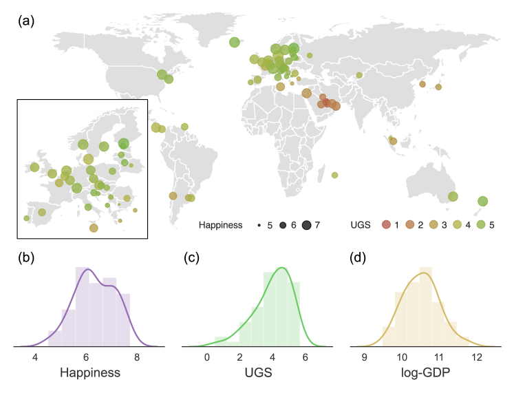
Figure 1: The distributions of urban green space and happiness over the world. (a) The map of urban green space and happiness in 60 developed countries. The size and color of circles represent the level of happiness and urban green space in a country, respectively. The markers are placed on the most populated cities of each country. (b-d) The histograms of (b) happiness, (c) urban green space (UGS) and (d) logarithmic GDP per capita (log-GDP). We use the logarithm of the total NDVI per capita as an indicator of urban green space, and the logarithm of GDP per capita as a measure of wealth.

We examine the global relationship between urban green space and happiness in 60 developed countries ranked by the Human Development Index. Using the Sentinel-2 satellite imagery dataset, we define each country’s urban green space score (UGS) as a logarithmic total vegetation index per capita in the most populated cities (i.e., those that include at least 10% of the national population). Among the various vegetation indices available, NDVI Miura et al. (2019) is used based on the robustness of the results for different tested indices. The happiness score and the gross domestic product based on purchasing power parity (GDP (PPP)) per capita of each country are from the World Happiness Report Helliwell et al. (2018) and the International Monetary Fund (IMF) estimation IMF (2018), respectively (see the Methods section and the Supplementary Information for details).

Figure 1(a) shows an overall view of urban green space and the happiness of countries around the world. This map highlights regional differences in the green space distribution due to climate; countries near the equator in tropical climates have relatively high UGS values, while countries located in the 20-30^∘ latitude range have exceptionally low UGS values due to the dry climate. UGS increases with latitude in higher-latitude regions. On the other hand, Northern and Western European and North American countries display relatively large happiness. Western Asian countries also show relatively high happiness with low UGS value, indicating that the relationship between happiness and green space is not trivial.

Figure 1(b-d) shows the distribution of happiness, UGS, and log-GDP, and they all show unimodal distributions with low skewness, which is appropriate for linear regression analyses. Note that the probability distributions of NDVI per capita and GDP per capita converge to a normal distribution after logarithmic scaling. Our comparison of several green space measures shows that the logarithmic NDVI per capita is most suitable for the following analysis in terms of its distribution and explanatory power. We hence choose the logarithmic NDVI per capita as the primary green space indicator in this research. (see Supplementary Information). We also use the logarithmic GDP per capita (PPP) (hereinafter referred to as the log-GDP) as a measure of the wealth of the country, as noted in the Happiness Report Helliwell et al. (2018).

Countries		All			Lower 30			Top 30
Model	(1)	(2)	(3)	(4)	(5)	(6)	(7)	(8)	(9)
log-GDP	1.0120***	-	1.1319***	0.9034**	-	0.8517*	-0.0809	-	0.2581
	(0.6603)		(0.6234)	(1.6305)		(1.7493)	(1.3559)		(1.0314)
UGS	-	0.1165	0.2249***	-	0.1497	0.0567	-	0.2785***	0.2946***
		(0.3545)	(0.2643)		(0.6042)	(0.6051)		(0.2313)	(0.2403)
Const	-4.2945**	5.9007***	-6.4709***	-3.3428	5.1767***	-3.0629	7.7712**	5.8110***	2.9312
	(6.9672)	(1.4910)	(6.8998)	(16.5490)	(2.6490)	(17.1094)	(14.8065)	(0.9455)	(11.5463)
Adjusted $R^{2}$	0.3832	0.00123	0.4786	0.1296	0.0012	0.1013	-0.0335	0.4457	0.4468
Observations	60	60	60	30	30	30	30	30	30

Table 1: The regression analysis for happiness, UGS, and log-GDP. The values denote the regression coefficients and the confidence intervals of each independent variable with its significance (i.e., ^***p¡0.01; ^**p¡0.05; ^*p¡0.1). The regression model (1-3), model (4-6) and model (7-9) are examined for the data of all countries, the lower 30 countries and the top 30 countries ranked by GDP, respectively.

As per-country wealth is an important indicator of its citizens’ quality of life, wealth (i.e., log-GDP) should be considered in analyzing urban green space and happiness. Our regression analysis finds that UGS, together with log-GDP, explains happiness. We make new observations from Table 1. Although UGS is not substantially correlated with happiness in the simple linear regression (i.e., model (2)), the multilinear model with log-GDP (i.e., model (3)) has a substantial increase in prediction ability compared to the simple regression analysis on log-GDP (i.e., model (1)). Therefore, urban green space adds explanatory power to the correlation between wealth and happiness across countries. The regression analyses with other green space-variant measures further confirm this result’s robustness, confirming a substantial increase in the adjusted R-squared value when including UGS in the regression. Specifically, UGS based on the logarithmic NDVI per capita shows the best regression performance (see the Supplementary Information for the results for the different measures).

III Urban green space is effective in rich countries

Our results show that happiness is correlated with urban green space and the GDP of a country. But, is this green space-happiness effect uniform across all countries? Previous studies on the marginal effect of income on happiness suggest that happiness may have a nonlinear relationship with GDP, presumably showing saturation after a specific GDP — a concept known as the Easterlin paradox Easterlin et al. (2010). This paradox tells us that increases in happiness through GDP reach a saturation point, yet what factors promote happiness beyond the saturation point is unknown.

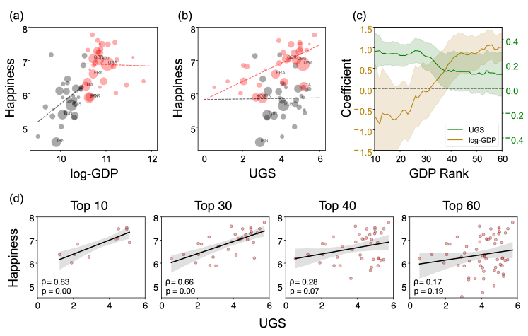
Figure 2: The effect of GDP on the green-happiness relation. (a, b) The relations of (a) log-GDP and happiness, and (b) urban green space (i.e., UGS) and happiness across 60 developed countries. The top 30 and the lower 30 countries ranked by GDP are sized by the population size and colored by red and black. The dotted lines are the linear fit for each GDP group. (c) Changes of coefficients between urban green space and happiness for different sets of GDP rank with increasing window size from top 10 to 60. (d) The rank correlations between UGS and happiness for the groups of increasing countries in the GDP rank order.

To test the Easterlin paradox, we repeated the analysis over clusters of countries grouped by GDP. Figure 2(a) shows a high correlation between GDP and happiness in the 30 lower-GDP countries (i.e., $\rho=0.40$), whereas the correlation is no longer evident in the 30 higher-GDP countries (i.e., $\rho=-0.04$). These results suggest that economic prosperity (as measured by GDP) is crucial for people’s happiness but fails to further promote happiness in rich countries. The GDP appears to reach a happiness-correlation threshold around the 30th wealthiest country, which corresponds to a GDP of 38,518 dollars. Previous research on the Easterlin paradox has stated that the GDP per capita can increase happiness until it reaches a certain threshold but cannot further increase happiness above that threshold. We observe a similar pattern for wealth and happiness across countries. On the other hand, happiness in the 30 wealthiest countries is well explained by urban green space. As shown in Figure 2(b), urban green space is positively correlated with happiness in the richest countries (i.e., $\rho=0.66,p<0.01$), but this correlation is not significant in the 30 lower-GDP countries (i.e., $\rho=0.19,p=0.32$). Thus, urban green space is a factor that further increases the happiness of a country after its GDP reaches a certain level.

The regressions for each of the 60 countries ranked by GDP in Table 1 confirm the individual effects of urban green space and GDP on happiness. GDP is the only substantial factor explaining happiness in the 30 lower-GDP countries (models 4-6). In contrast, for the 30 higher-GDP countries, happiness is explained only by the UGS (7-9). These findings suggest that GDP is critical for happiness until it reaches a certain GDP threshold (i.e., the Easterlin paradox), after which urban green space explains happiness better.

The correlation between UGS and happiness also corroborates the effect of UGS in rich countries. The correlation in Figure 2(d) decreases as more countries in the decreasing order of GDP are added. The correlation is substantial (i.e., $\rho$ is approximately 0.8) among the countries excluding the top 30. Figure 2(c) summarizes the effects of urban green space and GDP that cross over each other around the 30th wealthiest country. For the top 30 countries, urban green space has positive coefficients, but the GDP effect is not significant. These relationships are reversed for less affluent countries.

In summary, economic support seems to promote happiness until the essential requirements and living standards are met. However, economic success alone fails to add persistent promotion of happiness. After some level, urban green space appears to be related to other social factors that can further promote happiness.

IV Urban green space for social cohesion

Our findings highlight urban green space as an indicator that might be correlated with social factors promoting happiness beyond the achievement of economic success. The question then arises, which social factors connect urban green space with happiness? To identify this connection, we first examine the correlation between UGS and socioeconomic variables reported in the World Happiness Report: GDP per capita, social support, life expectancy, freedom, generosity, and perceptions of corruption. Of these six variables, only “social support” has a significantly positive correlation ($\rho=0.43,p<0.01$) with UGS as we can see from Fig. 3(a), implying that social support could mediate between urban green space and happiness. This relationship is consistent with several existing studies that suggested urban green space as a place of social cohesion Maas et al. (2009); Jennings and Bamkole (2019). On the other hand, as indicated by life expectancy, physical health does not display a significant relationship with green space ( $\rho=0.19,p=0.15$), contradicting common sense. The regression analysis on happiness with UGS and six socioeconomic variables also captures the interchangeability of urban green space and social support (see the Supplementary Information for details).

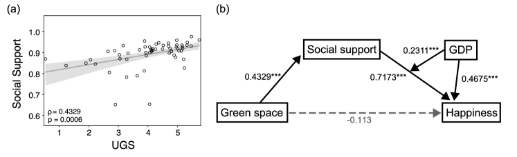
Figure 3: The moderated mediation model for UGS, happiness and socioeconomic indicators. (a) Scatter plot of social support and UGS across countries. (b) Diagram for the moderated mediation model. The boxes denote the model variables. Solid black arrows denote a statistically significant relationship between a pair of variables with the regression coefficient and the p-value (i.e., ***p¡0.01). The gray dashed arrow represents a non-significant relationship. Note that the coefficients are calculated with z-scores of the variables to compare the effect size directly.

Here, we employ a moderated mediation model Preacher et al. (2007) to characterize the complicated relationships among urban green space, social support, GDP, and happiness. In moderated mediation models, the moderator describes a variable’s conditional effect through the interaction term, and the mediator describes a variable’s indirect effect connecting the other two variables. Accordingly, moderated mediation models determine the pathway of directed interactions between multiple variables.

First, we examine the mediation effect of urban green space and social support as independent variables. The mediation regression model shows that social support mediates the relationship between urban green space and happiness such that (1) urban green space improves social support and (2) social support promotes happiness. The mediation effect is significant (3) only when GDP is considered in the model. Consequently, our moderated mediation model combining these three effects, shown in Fig. 3(b), presents the pathway by which green space affects happiness through social support, given that GDP moderates the effect of social support. If we describe this relationship in equations,

$$H=\beta_{0}+\beta_{1}M+\beta_{2}S+\beta_{3}SM,$$ (1)

$$S=\beta_{4}+\beta_{5}\ln{G}.$$ (2)

where $H$, $M$, $S$, and $G$ represent happiness, log-GDP, social support, and NDVI per capita, respectively, and the $\beta$ values denote the coefficients of the regression models (see the Supplementary Information for details).

Our moderated mediation model can be used to estimate the amount of urban green space required to increase happiness by a certain amount according to

$$\Delta H=\left(\beta_{1}^{\prime}+\beta_{2}^{\prime}M\right)\ln{\frac{G_{f}}{G_{i}}}.$$ (3)

In the equation 3, the required ratio of urban green spaces in a country decreases as its log-GDP increases. The required increase in urban green space per capita can be estimated for each country based on its current GDP value. For example, the United States needs an additional 36.1908 NDVI of urban green space per capita to increase its happiness score by 0.0546. In contrast, 3,416 USD per capita is required to achieve the same increment in happiness. Here, we used a 0.0546 happiness score as a reference value of $\Delta H$, which is the average value between happiness ranks. Note that the NDVI per capita is interpreted as a weighted area of green space, with a unit of $m^{2}$. Similarly, Qatar needs 0.4981 NDVI per capita or 7,556 dollars per capita, and South Korea needs 4.1332 NDVI per capita or 2,315 dollars per capita to achieve the reference happiness score increase.

V Discussion

This paper revealed a global relationship between urban green space and happiness in over 60 countries using high-resolution satellite imagery. Urban green space has a higher impact in developed countries (i.e., countries with higher GDPs), which suggests urban green space as a key to promoting happiness beyond economic success. Our moderated mediation model further elucidates this relationship as social support mediates the green-happiness relation, and GDP moderates social support and happiness. This sophisticated model could estimate additional green space needed to promote happiness for each country.

The current study newly defined the concept of UGS (urban green space score), which can be used to calculate the amount of green space at any spatial scale accounting for population density. We compared several green space measures and proposed to use the logarithmic NDVI per capita as a preferred measure of UGS. This index was validated through experiments and it makes it possible to investigate green space at a global level, allowing us to perform cross-sectional research on green space. Furthermore, the method obtaining UGS can be utilized to investigate any spatial areas such as blue space (i.e., aquatic environments such as lake and shore) Foley and Kistemann (2015); Raymond et al. (2016).

Our findings have multiple policy-level implications. First, public green space should be made accessible to urban dwellers to enhance social support. In doing so, one critical aspect is public safety. If public safety in urban parks is not guaranteed Groff and McCord (2012); Han et al. (2018), its positive role in social support and happiness may diminish. The meaning of public safety may change; for example, ensuring biological safety will be a priority in keeping the urban parks accessible during the COVID-19 pandemic Ugolini et al. (2020).In fact, the high indoor transmission rate of the virus Lolli et al. (2020) will increase awareness and importance of open spaces like urban parks. While some urban parks may be closed during lockdowns, some reports suggest that viewing them from home could also help relax stress during the pandemic Hedblom et al. (2019). Second, urban planning of public green space is needed for both developed and developing countries. While our findings confirmed a strong impact of urban green space on happiness in developed countries, the same positive effect holds for developing countries, albeit to a smaller degree. Furthermore, it is challenging or nearly impossible to secure land for green space after built-up areas are developed in cities. Therefore, urban planning for parks and green recovery (new greening in built-up areas) should be considered in developing economies where new cities and suburban areas rapidly expand Ewing (2008); Liu et al. (2020).

In addition to the above, recent climate changes can create substantial volatility in sustaining urban green space. Extreme events such as wildfires, floods, droughts, and cold waves could endanger urban forests around the world Allen et al. (2010). On the other hand, global warming could also accelerate tree growth in cities more than in rural areas due to the urban heat island effect Pretzsch et al. (2017). In the end, the environmental influence is bidirectional; urban green spaces affect local climates by reducing carbon dioxide levels Nowak et al. (2013) and providing a cooling effect inside the city that indirectly affects people’s well-being. Thus, we need more attention to predicting climate changes and discovering their impact on public places since the extreme changes could hamper the benefits of urban green space.

As an exciting future direction, satellite images of higher spatiotemporal resolutions can be used to compute urban green space scores. This paper focused on the correlation across countries fixed in time, given the short span of the Sentinel-2 dataset launched in 2015. A causal analysis could be done with satellite imagery data for a longer span. Also, our dataset does not cover all the countries in the world. Fortunately, our observations from the 30 lower-income countries anticipate the substantial effect of GDP in other developing countries excluded in our analysis. We have analyzed the highest-resolution public dataset of satellite imagery in this study. However, our method still has room for application to higher-resolution non-public datasets such as the household level (less than 10m resolution) available in the national-scale health dataset Houlden et al. (2017). Since satellite imagery cannot account for green space inside buildings (such as green walls), future research could quantify the effect of these mini-scale green spaces using computer vision Seiferling et al. (2017).

VI Methods

VI.1 Collecting happiness and remote sensing data

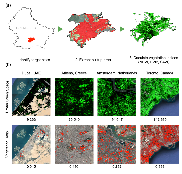
Figure 4: Measuring urban green spaces. (a) Measurement methods to compute the size of urban green space in each country. First, we find cities occupying more than 10 percent of the total population in a country. Then, we extract the built-up area of the cities with Copernicus global landcover data. Finally, we calculate vegetation indices (e.g., NDVI) within the area using Sentinel-2 satellite images.(b) Urban green space measured by the UGS (upper row) and the vegetation ratio (lower row) in four world cities.The red areas in the upper row indicate vegetation for the NDVI threshold of 0.4. The lower row images show the adjusted NDVI per capita (i.e., UGS) for every 10m by 10m pixel.

To identify the relationship between happiness and green space, we use happiness scores from the World Happiness Report Helliwell et al. (2018) and the NDVI scores from Sentinel-2 satellite imagery as remote sensing data. The World Happiness Report from 2018 covered 156 countries. The report provides an annual survey of how happy citizens perceive themselves to be and ranks the countries by happiness score. The score is the average of the participants’ responses asked to rate how happy they are on a scale from 0 and 10. While many socioeconomic indicators (e.g., unemployment and inequality) may affect happiness, not all of these factors are measured annually across 156 countries. The report instead describes happiness with six primary socioeconomic indicators: GDP per capita, social support, life expectancy, freedom to make life choices, generosity, and perceptions of corruption. For example, the social support variable is based on binary responses (yes/no) on a Gallup World Poll question: ”If you were in trouble, do you have relatives or friends you can count on to help you whenever you need them, or not?”

To quantify urban green space in global cities, we use the Sentinel-2 dataset that provides the highest spatial resolution (10 m) among the publicly available satellite imagery datasets (e.g., 30 m resolution in Landsat series) Beyer et al. (2014); Dadvand et al. (2016); Dzhambov et al. (2018); Liu et al. (2019). With this high resolution, we can identify granular green space, including street vegetation and home gardens that could not be detected in other public datasets. When using satellite imagery to detect small vegetation, it is critical to consider the season in which the images were obtained Beyer et al. (2014); Dadvand et al. (2016); Dzhambov et al. (2018); Liu et al. (2019). We use the images from summer: June to September 2018 for the Northern Hemisphere and December 2017 to February 2018 for the Southern Hemisphere. Satellite images with below 10% cloud cover were used; when such images could not be obtained for the study period, data from 2019 were used instead.

Normalized difference vegetation index (NDVI) is a well-known remote sensing indicator of green vegetation areas in satellite images Miura et al. (2019). It detects vegetation as the difference between near-infrared and red light, in the value range from -1 to +1. In general, high NDVI scores include urban green spaces such as official parks, backyards, street trees, mountains, riverbanks, golf courses, and urban farmlands. There are a few well-known variants of NDVI Markevych et al. (2017), such as the soil-adjusted vegetation index (SAVI) Huete (1988), which is corrected for soil brightness, and the enhanced vegetation index (EVI) Jiang et al. (2008), which is corrected for atmospheric effects. All NDVI, SAVI, and EVI2 scores can be calculated from the two spectral bands of Sentinel-2, red (band 4) and near-infrared (NIR, band 8), as follows:

$$NDVI=\frac{NIR-RED}{NIR+RED},$$ (4)

$$SAVI=\frac{(1+L)(NIR-RED)}{NIR+RED+L},$$ (5)

$$EVI2=2.5\frac{NIR-RED}{NIR+2.4RED+1}.$$ (6)

The robustness of the results for the three green space measures was verified using NDVI as the primary metric.

VI.2 Measuring the amount of green space

The vegetation indices are measured in three steps, as illustrated in Fig. 4(a). The first step is to identify target cities containing at least 10% of each country’s total population and represent the country’s overall happiness. The second step is to extract only the built-up areas within the identified cities’ administrative boundaries. As cities’ boundaries are historically and culturally constructed and often arbitrary, the cities’ size needs to be standardized; some cities include vast suburban areas (e.g., Istanbul) or natural areas (e.g., deserts in Dubai). Thus, referring to the global land cover data from the EU’s Copernicus Programme Buchhorn et al. (2020), we focus on urban built-up areas to quantify the urban green space. Finally, the vegetation indices (NDVI, EVI2, and SAVI) are calculated for the extracted urban areas.

The final step is to compute the amount of green space in each country, determined from the measured vegetation indices. Here, we define the amount of green space as the logarithm of the total NDVI of built-up areas in the target cities divided by the cities’ total population, called UGS, as a metric for urban green space. UGS is calculated as follows:

$$UGS=\log{\left(\frac{\sum_{c}\sum_{b(c)}NDVI(b)}{\sum_{c}N_{c}}\right)},$$ (7)

where $NDVI(b)$ is the value of NDVI of pixel $b$ within built-up areas $b(c)$ in city $c$ and $N_{c}$ is the population of city $c$. In this calculation, we adjusted negative NDVI values to zero Markevych et al. (2017) to prevent errors caused by the accumulation of negative values in areas next to bodies of water (see the Supplementary Information for the entire dataset).

Author contributions statement

M.C. and D.Y.W. conceived the research, I.H., W.-S.J. and M.C. designed the research, O.-H.K. and J.Y. collected the data, O.-H.K. performed the research, O.-H.K., I.H. and M.C. analysed the data, O.-H.K., I.H. and J.Y. wrote the manuscript. All authors reviewed the manuscript.

References

- de Vries et al. (2003) S. de Vries, R. A. Verheij, P. P. Groenewegen, and P. Spreeuwenberg, Environment and Planning A: Economy and Space 35, 1717 (2003).
- Dadvand et al. (2016) P. Dadvand, X. Bartoll, X. Basagaña, A. Dalmau-Bueno, D. Martinez, A. Ambros, M. Cirach, M. Triguero-Mas, M. Gascon, C. Borrell, et al., Environmental International 91, 161 (2016).
- UN (2015) UN, Sustainable Development Goals (2015), available at https://sdgs.un.org/goals. Date accessed 4 November 2020.
- de Vries et al. (2013) S. de Vries, S. M. E. van Dillen, P. P. Groenewegen, and P. Spreeuwenberg, Social Science & Medicine 94, 26 (2013).
- Liu et al. (2019) Y. Liu, R. Wang, G. Grekousis, Y. Liu, Y. Yuan, and Z. Li, Landsacpe and Urban Planning 190 (2019).
- Dzhambov et al. (2018) A. Dzhambov, T. Hartig, I. Markevych, B. Tilov, and D. Dimitrova, Environmental Research 160, 47 (2018).
- Maas et al. (2009) J. Maas, S. M. E. van Dillen, R. A. Verheij, and P. P. Groenewegen, Health & Place 15, 586 (2009).
- Jennings and Bamkole (2019) V. Jennings and O. Bamkole, International journal of environmental research and public health 16, 452 (2019).
- Kweon et al. (1998) B. S. Kweon, W. C. Sullivan, and A. R. Wiley, Environment and Behavior 30, 832 (1998).
- Maas et al. (2006) J. Maas, R. A. Verheij, P. P. Groenewegen, S. de Vries, and P. Spreeuwenberg, Journal of Epidemiology & Community Health 60, 587 (2006).
- MacKerron and Mourato (2013) G. MacKerron and S. Mourato, Global Environmental change 23, 992 (2013).
- Alcock et al. (2014) I. Alcock, M. P. White, B. W. Wheeler, L. E. Fleming, and M. H. Depledge, Environmental Science & Technology 48, 1247 (2014).
- Beyer et al. (2014) K. M. M. Beyer, A. Kaltenbach, A. Szabo, S. Bogar, F. J. Nieto, and K. M. Malecki, International Journal of Environmental Research and Public Health 11, 3453 (2014).
- Tsai et al. (2018) W.-L. Tsai, M. R. Mchale, V. Jennings, O. Marquet, J. A. Hipp, Y.-F. Leung, and M. F. Floyd, International Journal of Environmental Research and Public Health 15 (2018).
- Stigsdotter et al. (2010) U. K. Stigsdotter, O. Ekholm, J. Schipperijn, M. Toftager, F. Kamper-Jørgensen, and T. B. Randrup, Scandinavian Journal of Public Health 38, 411 (2010).
- EOS (2019) EOS, NDVI FAQ: ALL YOU NEED TO KNOW ABOUT NDVI (2019), available at https://eos.com/blog/ndvi-faq-all-you-need-to-know-about-ndvi/. Date accessed 22 June 2020.
- van den Berg et al. (2016) M. van den Berg, M. van Poppel, I. van Kamp, S. Andrusaityte, B. Balseviciene, M. Cirach, A. Danileviciute, N. Ellis, G. Hurst, D. Masterson, et al., Health & Place 38, 8 (2016).
- Markevych et al. (2017) I. Markevych, J. Schoierer, T. Hartig, A. Chudnovsky, P. Hystad, A. M. Dzhambov, S. de Vries, M. Triguero-Mas, M. Brauer, M. J. Nieuwenhuijsen, et al., Environmental Research 158, 301 (2017).
- Helliwell et al. (2018) J. F. Helliwell, R. Layard, and J. D. Sachs, New York: UN Sustainable Development Solutions Network (2018).
- Kahneman and Deaton (2010) D. Kahneman and A. Deaton, Proceedings of the National Academy of Sciences 107, 16489 (2010).
- Miura et al. (2019) T. Miura, S. Nagai, M. Takeuchi, K. Ichii, and H. Yoshioka, Scientific Reports 9 (2019).
- IMF (2018) IMF, World Economic Outlook Database (2018), available at https://www.imf.org/en/Publications/SPROLLS/world-economic-outlook-databases. Date accessed 16 November 2020.
- Easterlin et al. (2010) R. A. Easterlin, L. A. McVey, M. Switek, O. Sawangfa, and J. S. Zweig, Proceedings of the National Academy of Sciences 107, 22463 (2010).
- Preacher et al. (2007) K. J. Preacher, D. D. Rucker, and A. F. Hayes, Multivariate Behavioral Research 42, 185–227 (2007).
- Foley and Kistemann (2015) R. Foley and T. Kistemann, Health & Place 35, 157–165 (2015).
- Raymond et al. (2016) C. M. Raymond, S. Gottwald, and M. Kytta, Landscape and Urban Planning 153, 198–208 (2016).
- Groff and McCord (2012) E. Groff and E. S. McCord, Security journal 25, 1 (2012).
- Han et al. (2018) B. Han, D. A. Cohen, K. P. Derose, J. Li, and S. Williamson, American journal of preventive medicine 54, 352 (2018).
- Ugolini et al. (2020) F. Ugolini, L. Massetti, P. Calaza-Martínez, P. Cariñanos, C. Dobbs, S. K. Ostoić, A. M. Marin, D. Pearlmutter, H. Saaroni, I. Šaulienė, et al., Urban Forestry & Urban Greening 56, 126888 (2020).
- Lolli et al. (2020) S. Lolli, Y.-C. Chen, S.-H. Wang, and G. Vivone, Scientific Reports 10, 16213 (2020).
- Hedblom et al. (2019) M. Hedblom, B. Gunnarsson, B. Iravani, I. Knez, M. Schaefer, P. Thorsson, and J. N. Lundström, Scientific Reports 9, 10113 (2019).
- Ewing (2008) R. H. Ewing, Characteristics, Causes, and Effects of Sprawl: A Literature Review (Springer US, Boston, MA, 2008).
- Liu et al. (2020) X. Liu, Y. Huang, X. Xu, X. Li, X. Li, P. Ciais, P. Lin, K. Gong, A. D. Ziegler, A. Chen, et al., Nature Sustainability 3, 564 (2020).
- Allen et al. (2010) C. D. Allen, A. K. Macalady, H. Chenchouni, D. Bachelet, N. McDowell, M. Vennetier, T. Kitzberger, A. Rigling, D. D. Breshears, E. H. Hogg, et al., Forest Ecology and Management 259, 660 (2010).
- Pretzsch et al. (2017) H. Pretzsch, P. Biber, E. Uhl, J. Dahlhausen, G. Schütze, D. Perkins, T. Rötzer, J. Caldentey, T. Koike, T. van Con, et al., Scientific Reports 7 (2017).
- Nowak et al. (2013) D. J. Nowak, E. J. Greenfield, R. E. Hoehn, and E. Lapoint, Environmental Pollution 178, 229 (2013).
- Houlden et al. (2017) V. Houlden, S. Weich, and S. Jarvis, BMC public health 17, 460 (2017).
- Seiferling et al. (2017) I. Seiferling, N. Naik, C. Ratti, and R. Proulx, Landscape and Urban Planning 165, 93 (2017).
- Huete (1988) A. R. Huete, Remote Sensing of Environment 25, 295 (1988).
- Jiang et al. (2008) Z. Jiang, A. R. Huete, K. Didan, and T. Miura, Remote Sensing of Environment 112, 3833 (2008).
- Buchhorn et al. (2020) M. Buchhorn, B. Smets, L. Bertels, B. De Roo, M. Lesiv, N.-E. Tsendbazar, M. Herold, and S. Fritz, Copernicus Global Land Service: Land Cover 100m: collection 3 epoch 2015, Globe (2020), available at https://lcviewer.vito.be/download.