An Adaptive Rank Continuation Algorithm for General Weighted Low-rank Recovery

\noindentAbstract

This paper is devoted to proposing a general weighted low-rank recovery model and designing a fast SVD-free computational scheme to solve it. First, our generic weighted low-rank recovery model unifies several existing approaches in the literature. Moreover, our model readily extends to the non-convex setting. Algorithm-wise, most first-order proximal algorithms in the literature for low-rank recoveries require computing singular value decomposition (SVD). As SVD does not scale appropriately with the dimension of the matrices, these algorithms become slower when the problem size becomes larger. By incorporating the variational formulation of the nuclear norm into the sub-problem of proximal gradient descent, we avoid computing SVD, which results in significant speed-up. Moreover, our algorithm preserves the rank identification property of nuclear norm [34] which further allows us to design a rank continuation scheme that asymptotically achieves the minimal iteration complexity. Numerical experiments on both toy examples and real-world problems, including structure from motion (SfM) and photometric stereo, background estimation, and matrix completion, demonstrate the superiority of our proposed algorithm.

Key words. Low-rank recovery, weighted low-rank, nuclear norm, singular value decomposition, proximal gradient descent, alternating minimization, rank identification/continuation

AMS subject classifications. 49J52, 65K05, 65K10, 90C06, 90C30

1 Introduction

Low-rank matrix recovery is an important problem to study as it covers many interesting problems arising from diverse fields including machine learning, data science, signal/image processing, and computer vision, to name a few. The goal of low-rank recovery is to recover or approximate the targeted matrix $\mathring{X}\in\mathbb{R}^{m\times n}$ whose rank is much smaller than its dimension. For example, matrix completion [56, 13], structure from motion [45], video segmentation [66, 29, 63], image processing and signal retrieval [26, 61] exploit the inherent low-rank structure of the data.

For many problems of interests, instead of accessing the data $\mathring{X}$ directly, often we can only observe it through some agent (e.g. a linear operator) $\Psi$. A general observation model takes the following form

$$F=\Psi(\mathring{X})+\varepsilon,$$ (1)

where $\Psi:\mathbb{R}^{m\times n}\to\mathbb{R}^{d\times\ell}$ is the (observation) operator which is assumed to be bounded linear. For example, in the compressed sensing scenario, $\Psi$ returns a linear measurement of $\mathring{X}$ which is a $d$-dimensional vector [26]; for matrix completion $\Psi$ is a binary mask [13]. In the above model, variable $\varepsilon\in\mathbb{R}^{d\times\ell}$ denotes additive noise (e.g. white Gaussian) and $F\in\mathbb{R}^{d\times\ell}$ is the obtained noise contaminated observation.

Over the years, numerous low-rank recovery models are proposed in the literature, for example [40, 65, 61, 64, 63, 15], to mention a few. When the rank of $\mathring{X}$ is available, one can consider the following rank constrained weighted least square

$$\min_{X\in\mathbb{R}^{m\times n}}~{}{{\frac{\raisebox{0.41669pt}{\footnotesize$1$}}{\raisebox{-1.24994pt}{\footnotesize$2$}}}}\|\big{(}{\Psi(X)-F}\big{)}\odot W\|^{2}\quad\mathrm{such~{}that}\quad\mathrm{rank}(X)\leq r,$$ (2)

where $r=\mathrm{rank}(\mathring{X})$ is the rank of $\mathring{X}$, $W\in\mathbb{R}^{d\times l}$ is a non-negative weight matrix, and $\odot$ is the Hadamard product. The motivation of considering a weight $W$ is such that (2) can handle more general noise model $\varepsilon$, rather than mere Gaussian noise [16, 22, 23]. A clear limitation of (2) is that, for many problems it is in general impossible to know $\mathrm{rank}(\mathring{X})$ a priori. As a result, instead of using rank as constraint, one can penalize it to the objective which results in rank regularized recovery model

$$\min_{X\in\mathbb{R}^{m\times n}}~{}{{\frac{\raisebox{0.41669pt}{\footnotesize$1$}}{\raisebox{-1.24994pt}{\footnotesize$2$}}}}\|\big{(}{\Psi(X)-F}\big{)}\odot W\|^{2}+\tau\mathrm{rank}(X),$$ (3)

where $\tau>0$ is the regularization parameter. Though avoids the estimation of $r$, one needs to choose $\tau$ properly. Moreover, due to rank function, (2) and (3) are non-convex, imposing challenges to both theoretical analysis and algorithmic design.

In literature, a popular approach to avoid non-convexity is to replace the rank function with its convex surrogate—the nuclear norm (a.k.a. trace norm) [36, 12]. Correspondingly, we obtain the following nuclear norm constrained form of (2):

$$\min_{X\in\mathbb{R}^{m\times n}}~{}{{\frac{\raisebox{0.41669pt}{\footnotesize$1$}}{\raisebox{-1.24994pt}{\footnotesize$2$}}}}\|\big{(}{\Psi(X)-F}\big{)}\odot W\|^{2}\quad\mathrm{such~{}that}\quad\|X\|_{*}\leq c,$$ (4)

where $c$ is a predefined constant, e.g. $c=\|\mathring{X}\|_{*}$ if possible. Consequently, for (3), we arrive at the following unconstrained nuclear norm regularized recovery model

$$\min_{X\in\mathbb{R}^{m\times n}}~{}{{\frac{\raisebox{0.41669pt}{\footnotesize$1$}}{\raisebox{-1.24994pt}{\footnotesize$2$}}}}\|\big{(}{\Psi(X)-F}\big{)}\odot W\|^{2}+\tau\|X\|_{*}.$$ (5)

Note that, besides the weighted $\ell_{2}$ loss, one can also consider the general loss function $f(X,F,W)$ which gives the following recovery model (similar to [31, 52])

$$\min_{X\in\mathbb{R}^{m\times n}}~{}f(X,F,W)+\tau\|X\|_{*}.$$ (6)

For the rest of the paper, we mainly focus on model (5) and only present a short discussion of (6) in Section 2.3.

1.1 Related work

Our recovery model (5) is connected with several established work in the literature, and moreover covers some as special cases. Therefore in what follows, we present a short overview of literature study.

Trace LASSO.

When the entries of $W$ are all $1$’s, problem (5) becomes the Trace LASSO considered in [25], i.e. nuclear norm regularized least square. For this case, $\varepsilon$ corresponds to additive white Gaussian noise. When $\Psi\in\mathbb{R}^{d\times m},\,F\in\mathbb{R}^{d\times n}$ and $W=\mathbf{1}\in\mathbb{R}^{d\times n}$, (5) becomes

$$\min_{X\in\mathbb{R}^{m\times n}}~{}{{\frac{\raisebox{0.41669pt}{\footnotesize$1$}}{\raisebox{-1.24994pt}{\footnotesize$2$}}}}\|\Psi X-F\|^{2}+\tau\|X\|_{*},$$ (7)

which is studied in [48]. Examples of (7) include multivariate linear regression, multi-class classification and multi-task learning [48]. As proposed in [30, 31], one can also consider a general loss function $f(X,F)$ (as a special case of (6)) to solve

$$\min_{X\in\mathbb{R}^{m\times n}}~{}f(X,F)+\tau\|X\|_{*},$$ (8)

For different choice of $f(X,F)$ in (8), one can recover affine-rank minimization [57, 40], regularized semi-definite linear least squares [52], etc.

Weighted low-rank recovery.

For the case $W$ is a general non-negative weight, there is also a train of works in the literature. For most of them, $\Psi$ is an identity operator. We start with rank constraint case

$$\min_{X\in\mathbb{R}^{m\times n}}~{}{{\frac{\raisebox{0.41669pt}{\footnotesize$1$}}{\raisebox{-1.24994pt}{\footnotesize$2$}}}}\|(F-X)\odot W\|^{2}\quad\mathrm{such~{}that}\quad\mathrm{rank}(X)\leq r,$$ (9)

which is well-studied in the literature under different settings [39, 53, 54, 43, 58]. In [42], instead of considering a generic weight $W$, the authors proposed a general matrix induced weighted norm

$$\min_{X\in\mathbb{R}^{m\times n}}\|F-X\|_{Q}^{2}\quad\mathrm{such~{}that}\quad\mathrm{rank}(X)\leq r,$$ (10)

where ${Q\in{\mathbb{R}}^{mn\times mn}}$ is symmetric positive definite and

$${\|F-X\|_{Q}^{2}\overset{\text{def}}{=}{\rm vec}(F-X)^{\top}Q{\rm vec}(F-X)}$$

with ${\rm vec}(\cdot)$ being an operator which maps the entries of $\mathbb{R}^{m\times n}$ to vectors in $\mathbb{R}^{mn\times 1}$ by stacking the columns. We refer to [16, 42, 22, 23, 49, 20] and the references therein for more discussions. If we lift the constraint to the objective function as for (3), we get the problem below:

$$\min_{X\in\mathbb{R}^{m\times n}}{{\frac{\raisebox{0.41669pt}{\footnotesize$1$}}{\raisebox{-1.24994pt}{\footnotesize$2$}}}}\|(X-F)\odot W\|^{2}+\tau{\rm rank}(X),$$ (11)

which is studied in [21, 16]. The latest addition to this class of problems is the weighted singular value thresholding studied in [17] which takes the form:

$$\min_{X\in\mathbb{R}^{m\times n}}{{\frac{\raisebox{0.41669pt}{\footnotesize$1$}}{\raisebox{-1.24994pt}{\footnotesize$2$}}}}\|(X-F)W\|^{2}+\tau\|X\|_{*},$$ (12)

where $W\in\mathbb{R}^{n\times n}$ is a weight matrix. Let $U\Sigma V^{\top}$ be a SVD of $W$ with $\Sigma={\rm diag}(\sigma_{1}\;\sigma_{2}\cdots\sigma_{n})$. Applying the unitary invariance of the norms (and by the change of variable $X\to XU$), problem (12) becomes

$$\min_{X\in\mathbb{R}^{m\times n}}{{\frac{\raisebox{0.41669pt}{\footnotesize$1$}}{\raisebox{-1.24994pt}{\footnotesize$2$}}}}\|(X-FU)\Sigma\|^{2}+\tau\|X\|_{*},$$ (13)

which moreover can be equivalently written as

$$\min_{X\in\mathbb{R}^{m\times n}}{{\frac{\raisebox{0.41669pt}{\footnotesize$1$}}{\raisebox{-1.24994pt}{\footnotesize$2$}}}}\|(X-FU)\odot W_{\Sigma}\|^{2}+\tau\|X\|_{*},$$ (14)

where ${W_{\Sigma}=(\sigma_{1}\mathbf{1};\;\sigma_{2}\mathbf{1};\cdots;\sigma_{n}\mathbf{1})\in\mathbb{R}^{m\times n}}$ and $\mathbf{1}\in\mathbb{R}^{m\times 1}$ is the vector of all $1$’s. In Table 1 below, we summarize the above formulations studied in the literature to highlight the difference and connections between them.

Name	Formulation	Reference
SVD/PCA	$\min_{X:{\rm rank}(X)\leq r}\tfrac{1}{2}\|X-F\|^{2}$	[24, 32]
SVT	$\min_{X}\tau\|X\|_{*}+\|X-F\|^{2}$	[12]
Weighted low-rank (WLR)	$\min_{X:{\rm rank}(X)\leq r}\tfrac{1}{2}\|(X-F)\odot W\|^{2}$	[54, 53, 39]
General WLR (GWLR)	$\min_{X:{\rm rank}(X)\leq r}\tfrac{1}{2}\|X-F\|^{2}_{Q}$	[42, 44]
Weighted SVD	$\min_{X}\mathrm{rank}(X)+\tfrac{1}{2}\|(X-F)W\|^{2}$	[21, 16]
Weighted SVT (WSVT)	$\min_{X}\tau\|X\|_{*}+\tfrac{1}{2}\|(X-F)W\|^{2}$	[21, 16]
Nuclear norm regularized GWLR	$\min_{X}\tau\|X\|_{*}+\tfrac{1}{2}\|(\Psi X-F)\odot W\|^{2}$	This work
Nuclear norm constrained	$\min_{X:\|X\|_{*}\leq t/2}f(X)$	[30, 40, 13]
Trace norm minimization	$\min_{X}f(X)+\tau\|X\|_{*}$	[31, 11, 62, 64]

Table 1: SVT, weighted low-rank approximation and their variants.

1.2 Contributions

In this paper, we propose a general model (5) for low-rank recovery. Based on the variational formulation of nuclear norm, we propose an efficient algorithm which avoids computing SVD. More precisely, our contributions include the following aspects.

(i) A generic low-rank recovery model.

We propose general low-rank recovery models which covers several existing works as special cases. We provide a detailed comparison of our problem with the existing ones, both analytically and empirically. We believe problem (5) with our dedicated structure dependent analysis should be studied as a standalone problem to close the existing knowledge gap.

(ii) An efficient adaptive rank continuation algorithm.

In the literature, numerous numerical schemes can be applied to solve (5), since it is the sum of a smooth function and a non-smooth one. However, most of these algorithms require computing SVD, which does not scale properly with the dimension of the problem [17, 31, 48, 45]. To efficiently solve (5), we propose an SVD-free method (see Algorithm 1). By combing proximal gradient descent [37] and the variational characteristic of nuclear norm, we design a “proximal gradient & alternating minimization method” which we coin as ProGrAMMe. Our algorithm can also be applied to solve the general model (6) if the loss function $f(X,F,W)$ is smoothly differentiable with gradient being Lipschitz continuous. Moreover, our algorithm can be easily extended to the non-convex loss function case.

Based on the result of [34], we show that the sequence generated by Algorithm 1 can find the rank of the minimizer (to which the generated sequence converges) in finite number of iterations, which we call rank identification property. In turn, we design a rank continuation technique which leads to Algorithm 2. Compare to Algorithm 1, rank continuation is less sensitive to initial parameter, and asymptotically achieves the minimal per iteration complexity.

(iii) Numerical comparisons.

We evaluate our algorithms against 15 state-of-the-art weighted and unweighted low-rank approximation methods on various tasks, including structure from motion (SfM) and photometric stereo, background estimation from fully and partially observed data, and matrix completion. In these problems, different weights are used as deem fit—from binary weights to random large weights. We observed in all the tasks our weighted low-rank algorithm performs either better or is as good as the other algorithms. This indicates that our algorithm is robust and scalable to both binary and general weights on a diverse set of tasks.

1.3 Notions and definitions

Throughout the paper, $\mathbb{R}^{n}$ is a finite dimensional Euclidean space equipped with scalar product $\langle\cdot,\,\cdot\rangle$ and induced norm $\|{\cdot}\|$. We abuse the notation $\|{\cdot}\|$ for the Frobenius norm when $\cdot$ is a matrix. $\mathrm{Id}_{n}$ denotes the identity operator on $\mathbb{R}^{n}$. Let $S\subset\mathbb{R}^{n}$ be a non-empty close compact set, then $\mathrm{ri}(S)$ denotes its relative interior, and $\mathrm{par}(S)$ is the subspace which is parallel to $\mathrm{span}(S)$. The sub-differential of a proper closed convex function $g:\mathbb{R}^{n}\to\mathbb{R}\cup\{+\infty\}$ is a set-valued mapping defined by $\partial g:\mathbb{R}^{n}\rightrightarrows\mathbb{R}^{n},~{}x\mapsto\big{\{}v\in\mathbb{R}^{n}|g(x^{\prime})\geq g(x)+\langle v,\,x^{\prime}-x\rangle,\,\forall x^{\prime}\in\mathbb{R}^{n}\big{\}}$.

Definition 1.1.

The proximal mapping (or proximal operator) of a proper closed convex function $g:\mathbb{R}^{n}\to\mathbb{R}\cup\{+\infty\}$ is defined as: let $\gamma>0$

$${\rm prox}_{\gamma g}(y)=\arg\min_{x}\big{\{}\gamma g(x)+{{\frac{\raisebox{0.41669pt}{\footnotesize$1$}}{\raisebox{-1.24994pt}{\footnotesize$2$}}}}\|x-y\|_{2}^{2}\big{\}}.$$ (15)

For nuclear norm, its proximal mapping is singular value thresholding (SVT) [12], which is the lifting of vector soft-shrinkage thresholding to matrix [7].

Lemma 1.1 (Variational formulation of nuclear norm [50, 51]).

Let $X\in\mathbb{R}^{m\times n}$ and $U\in\mathbb{R}^{m\times r},V\in\mathbb{R}^{r\times n}$ with $r\geq\mathrm{rank}(X)$. We can write

$$\|X\|_{*}=\min_{\begin{subarray}{c}X=UV\\ U\in\mathbb{R}^{m\times r},V\in\mathbb{R}^{r\times n}\end{subarray}}\|U\|\|V\|=\min_{\begin{subarray}{c}X=UV\\ U\in\mathbb{R}^{m\times r},V\in\mathbb{R}^{r\times n}\end{subarray}}{{\frac{\raisebox{0.41669pt}{\footnotesize$1$}}{\raisebox{-1.24994pt}{\footnotesize$2$}}}}(\|U\|^{2}+\|V\|^{2}).$$

Paper organization

The rest of the paper is organized as following. In Section 2, we describe our proposed algorithm ProGrAMMe (Algorithm 1) and discuss its global convergence. In Section 3, we show the rank identification property of Algorithm 1 and then propose a rank continuation strategy (Algorithm 2). Numerical experiments are provided in Section 4, followed by the conclusion of this paper.

2 An SVD-free algorithm

Problem (5) is the composition of a smooth term and a non-smooth term. In the literature, numerical methods for such a structured problem are well studied, such as proximal gradient descent [37] (a.k.a. Forward–Backward splitting) and its various variants including the celebrated FISTA [6, 14]. Indeed, our problem (5) can be handled by proximal gradient descent. However, such a method requires repeated SVD computation, which can significantly slow down its performance in many practical scenarios where the data size is large. Therefore, in this section, by combining proximal gradient descent and the variational formulation of nuclear norm (c.f., Lemma 1.1), we propose a SVD-free method for solving (5).

2.1 Proposed algorithm

In this part, we provide a detailed derivation of our algorithm, which is a combination of proximal gradient descent, alternating minimization, and inertial acceleration. For convenience, denote $f(X)=\frac{1}{2}\|(\Psi(X)-F)\odot W\|^{2}$ and $g(X)=\|X\|_{*}$.

Step 1 - Inertial proximal gradient descent.

The first step to derive our algorithm is applying an inertial proximal gradient descent [37, 34] to solve problem (5). Since $\Psi$ is a bounded linear mapping, we have the following simple lemma.

Lemma 2.1.

Let $\widetilde{W}=W\odot W$. The loss $f(X)$ is smoothly differentiable with its gradient given by

$$\nabla f(X)=\nabla\Psi(X)\big{(}{(\Psi(X)-F)\odot\widetilde{W}}\big{)},$$

which is $L$-Lipschitz continuous with $\displaystyle{L=\|\nabla\Psi(X)\|^{2}\max_{i,j}\widetilde{W}_{i,j}}$.

Below we provide two examples of $\nabla\Psi(X)$:

• In compressed sensing scenario, $\Psi\in\mathbb{R}^{d\times mn}$ is a linear measurement matrix,

  $$\Psi(X)=\Psi\mathrm{vec}(X)\quad\mathrm{and}\quad\|\nabla\Psi(X)\|=\|\Psi\|.$$

• For matrix completion problem, $\Psi\in\mathbb{R}^{m\times n}$ is a binary mask, and

  $$\Psi(X)=\Psi\odot X\quad\mathrm{and}\quad\|\nabla\Psi(X)\|=1.$$

In the literature, a routine approach to solve (5) is inertial proximal gradient descent. Let $X_{0}\in\mathbb{R}^{m\times n}$ be an arbitrary starting point, we consider the following iteration

$$Y_{k} =X_{k}+a_{k}(X_{k}-X_{k-1}),$$ (16)

$${Z}_{k} =Y_{k}-\gamma\nabla\Psi(Y_{k})\big{(}{(\Psi(Y_{k})-F)\odot\widetilde{W}}\big{)},$$

$$X_{k+1} ={\arg\min}_{X\in\mathbb{R}^{m\times n}}\tau\|X\|_{*}+{{\frac{\raisebox{0.41669pt}{\footnotesize$1$}}{\raisebox{-1.24994pt}{\footnotesize$2\gamma$}}}}\|X-{Z}_{k}\|^{2},$$

where $a_{k}\in[0,1]$ is the inertial parameter, $\gamma\in]0,2/L[$ is the step-size. Iteration (16) is a special case of the general inertial scheme proposed in [34], and we refer to [34] and the references therein for more discussion on inertial schemes.

Step 2 - Alternating minimization.

As computing the proximal mapping of nuclear norm requires SVD, the goal of second step is to avoid SVD in solving SVT of $Z_{k}$ by incorporating the variational formulation of nuclear norm. To this end, the subproblem of (16) reads

$$\min_{X\in\mathbb{R}^{m\times n}}\tau\|X\|_{*}+{{\frac{\raisebox{0.41669pt}{\footnotesize$1$}}{\raisebox{-1.24994pt}{\footnotesize$2\gamma$}}}}\|X-{Z}_{k}\|^{2}.$$ (17)

By plugging in the variational formulation of nuclear norm, we arrive at the following constrained minimization problem: let $r>\mathrm{SVT}_{\tau\gamma}(Z_{k})$

$$\min_{X\in\mathbb{R}^{m\times n},U\in\mathbb{R}^{m\times r},V\in\mathbb{R}^{r\times n}}{{\frac{\raisebox{0.41669pt}{\footnotesize$1$}}{\raisebox{-1.24994pt}{\footnotesize$2$}}}}\|X-{Z}_{k}\|^{2}+{{\frac{\raisebox{0.41669pt}{\footnotesize$\tau\gamma$}}{\raisebox{-1.24994pt}{\footnotesize$2$}}}}\left(\|U\|^{2}+\|V\|^{2}\right)\;{\rm such\;that\;}X=UV.$$ (18)

Instead of considering the augmented Lagrangian multiplier of the constraint [11], we directly substitute the constraint $X=UV$ in the objective, which leads to

$$\min_{U\in\mathbb{R}^{m\times r},V\in\mathbb{R}^{r\times n}}{{\frac{\raisebox{0.41669pt}{\footnotesize$1$}}{\raisebox{-1.24994pt}{\footnotesize$2$}}}}\|UV-{Z}_{k}\|^{2}+{{\frac{\raisebox{0.41669pt}{\footnotesize$\tau\gamma$}}{\raisebox{-1.24994pt}{\footnotesize$2$}}}}\left(\|U\|^{2}+\|V\|^{2}\right),$$ (19)

which is a smooth, bi-convex optimization problem in each component $U$ and $V$.

Different from (17), problem (19) does not admits closed form solution. However, when either $U$ or $V$ is fixed, the problem becomes a simple least square. Hence we can solve (19) via a simple alternating minimization, namely a two block Gauss-Seidel iteration [3]: given $U_{0}\in\mathbb{R}^{m\times r},V_{0}\in\mathbb{R}^{r\times n}$

$$U_{i+1} ={{Z}_{k}}V_{i}^{\top}\big{(}V_{i}V_{i}^{\top}+{\tau\gamma}\mathrm{Id}_{r}\big{)}^{-1},$$ (20)

$$V_{i+1} =\big{(}U_{i+1}^{\top}U_{i+1}+{\tau\gamma}\mathrm{Id}_{r}\big{)}^{-1}U_{i+1}^{\top}{{Z}_{k}},$$

where $\mathrm{Id}_{r}$ denotes the identity operator on $\mathbb{R}^{r}$. Substituting (20) into (16) as an inner loop, we obtain the following iterative scheme: let $I\in\mathbb{N}_{+}$

$${Z}_{k}=Y_{k}-\gamma\nabla\Psi(Y_{k})\big{(}{(\Psi(Y_{k})-F)\odot\widetilde{W}}\big{)},$$ (21)

Initialize $$U_{0},V_{0} i=0,\ldots,I-1$$. For :

$$\left\lfloor\begin{aligned} U_{i+1}&={{Z}_{k}}V_{i}^{\top}\big{(}{V_{i}V_{i}^{\top}+{\tau\gamma}\mathrm{Id}_{r}}\big{)}^{-1},\\ V_{i+1}&=\big{(}{U_{i+1}^{\top}U_{i+1}+{\tau\gamma}\mathrm{Id}_{r}}\big{)}^{-1}U_{i+1}^{\top}{{Z}_{k}},\end{aligned}\right.$$

$$X_{k+1}=U_{I}V_{I}.$$

Assembling the above steps, we obtain our proposed algorithm, proximal gradient & alternating minimization method, which we call ProGrAMMe and is summarized below in Algorithm 1.

1:  Compute $\widetilde{W}=W\odot W,~{}L$ and et $\gamma\in]0,2/L[$; Choose $r>0$ and $I\in\mathbb{N}_{+}$;

2:  while not convergent do

3:     $Y_{k}=X_{k}+a_{k}(X_{k}-X_{k-1})$,$//$inertial step$//$     

4:     ${Z}_{k}=Y_{k}-\gamma\nabla\Psi(Y_{k})\big{(}{(\Psi(Y_{k})-F)\odot\widetilde{W}}\big{)}$,$//$gradient descent$//$     

5:     Initialize $U_{0}\in\mathbb{R}^{m\times r},V_{0}\in\mathbb{R}^{r\times n}$,

6:     for $i=1,...,I-1$ do$//$inner loop$//$     

7:       $U_{i+1}={{Z}_{k}}V_{i}^{\top}(V_{i}V_{i}^{\top}+{\tau\gamma}\mathrm{Id}_{r})^{-1}$,

8:       $V_{i+1}=(U_{i+1}^{\top}U_{i+1}+{\tau\gamma}\mathrm{Id}_{r})^{-1}U_{i+1}^{\top}{{Z}_{k}}$,

9:     end for

10:     $X_{k+1}=U_{I}V_{I}$.

11:  end while

12:  return  $X_{k+1}$

Algorithm 1 A Proximal Gradient & Alternating Minimization Method (ProGrAMMe)

Remark 2.2.

 

• One highlight of our algorithm is that, via variational formulation of nuclear norm, we relaxed the convex subproblem (17) to a non-convex (19) problem.

• Every step of Algorithm 1 requires initializing $U_{0},V_{0}$ for the inner step, and the simplest way is using the $U_{I},V_{I}$ from the last step.

• For the controlling parameter $r$, theoretically it does not make any difference as long as it is larger than the rank of the solution of (5). However, practically it is crucial to the performance of Algorithm 1. Detailed discussion is provided in Section 3.

Remark 2.3.

In the literature, several SVD-free approaches were proposed. For example, variational formulation was also considered in [11] and the resulted problem was solved by method of Lagrange multiplier while we directly plug the constraint into the objective. In [64], a dual characterization of the nuclear norm was used and a SVD-free gradient descent was designed. The benefits of our approach, as we shall see later, are simple convergence analysis (see Secsion 2.2) and extensions to more general settings (see Section 2.3).

Remark 2.4 (Per iteration complexity).

Comparing Algorithm 1 to proximal gradient descent (16), the only difference is Line 5-9. For proximal gradient descent, since SVD is needed, the iteration complexity each step is $O(mn\min\{m,n\})$. For Algorithm 1, suppose $I=1$, the complexity of Line 7-8 is $O((m+n+r)r^{2})$. It can be concluded that, the smaller the value of $r$ (still larger than the rank of the solutions), the lower the per iteration complexity of Algorithm 1. As a result, the choice of $r$ is crucial to the practical performance of Algorithm 1. Therefore, in Section 3, a detailed discussion is provided on how to choose $r$.

2.1.1 Relation with existing work

Our algorithm is closely related with proximal splitting method and its variants, as our first step to derive Algorithm 1 is the inertial proximal gradient descent (for example, proximal gradient descent [37] and its accelerated versions including FISTA [6, 14], as in [52, 57, 31] where FISTA was adopted to solving low-rank recovery problem).

Our model (5) and Algorithm 1 share similarities with those of [10, 15, 11], but there are some fundamental differences. First of all, all these works consider only the case $\Psi=\mathrm{Id}$, i.e. $\Psi$ is an identity mapping

$$\min_{X}{{\frac{\raisebox{0.41669pt}{\footnotesize$1$}}{\raisebox{-1.24994pt}{\footnotesize$2$}}}}\|(X-F)\odot W\|^{2}+\tau\|X\|_{*}.$$ (22)

In [10, 11], the authors consider directly applying matrix factorization to (22) which results in: let $r>0$

$$\min_{U\in\mathbb{R}^{m\times r},V\in\mathbb{R}^{r\times n}}{{\frac{\raisebox{0.41669pt}{\footnotesize$1$}}{\raisebox{-1.24994pt}{\footnotesize$2$}}}}\|(UV-F)\odot W\|^{2}+{{\frac{\raisebox{0.41669pt}{\footnotesize$\tau$}}{\raisebox{-1.24994pt}{\footnotesize$2$}}}}\left(\|U\|^{2}+\|V\|^{2}\right),$$ (23)

which is a smooth and bi-convex optimization problem. Our approach, on the other hand, only consider applying matrix factorization for the subproblem of proximal gradient descent (16).

It is worth noting that (23) shares the same continuous property as (19), hence can by handled by alternating minimization algorithm. Both (23) and (19) are also special cases of the following non-convex problem

$$\min_{U,V}f(U,V)+\tau_{1}g_{1}(U)+\tau_{2}g_{2}(V)$$ (24)

where $f(U,V)$ is differentiable with Lipschitz continuous gradient, $\tau_{1},\tau_{2}>0$ are regularization parameters and $g_{1}(\cdot),\,g_{2}(\cdot)$ are (non-smooth) regularization terms for $U,V$, respectively. Problem (24) was well studied in [2, 8]; for instance, the following algorithm was proposed in [2]:

$$U_{k+1} =\arg\min_{U\in\mathbb{R}^{m\times r}}~{}\big{\{}f(U,V_{k})+\tau_{1}g_{1}(U)+{{\frac{\raisebox{0.41669pt}{\footnotesize$1$}}{\raisebox{-1.24994pt}{\footnotesize$2\alpha$}}}}\|U-U_{k}\|^{2}\big{\}},$$

$$V_{k+1} =\arg\min_{V\in\mathbb{R}^{r\times n}}~{}\big{\{}f(U_{k+1},V)+\tau_{2}g_{2}(V)+{{\frac{\raisebox{0.41669pt}{\footnotesize$1$}}{\raisebox{-1.24994pt}{\footnotesize$2\gamma$}}}}\|V-V_{k}\|^{2}\big{\}},$$

where $\alpha,\gamma>0$ are parameters. Specializing to the case of (23), we get

$$U_{k+1} =\arg\min~{}\Big{\{}{{\frac{\raisebox{0.41669pt}{\footnotesize$1$}}{\raisebox{-1.24994pt}{\footnotesize$2$}}}}\|(UV_{k}-F)\odot W\|^{2}+{{\frac{\raisebox{0.41669pt}{\footnotesize$\tau$}}{\raisebox{-1.24994pt}{\footnotesize$2$}}}}\|U\|^{2}+{{\frac{\raisebox{0.41669pt}{\footnotesize$1$}}{\raisebox{-1.24994pt}{\footnotesize$2\alpha$}}}}\|U-U_{k}\|^{2}\Big{\}},$$

$$V_{k+1} =\arg\min~{}\Big{\{}{{\frac{\raisebox{0.41669pt}{\footnotesize$1$}}{\raisebox{-1.24994pt}{\footnotesize$2$}}}}\|(U_{k+1}V-F)\odot W\|^{2}+{{\frac{\raisebox{0.41669pt}{\footnotesize$\tau$}}{\raisebox{-1.24994pt}{\footnotesize$2$}}}}\|V\|^{2}+{{\frac{\raisebox{0.41669pt}{\footnotesize$1$}}{\raisebox{-1.24994pt}{\footnotesize$2\gamma$}}}}\|V-V_{k}\|^{2}\Big{\}}.$$

It can be observed that, though sharing similarities, our proposed algorithm is different from the above schemes. Same for the algorithm proposed in [8].

2.2 Global convergence of Algorithm 1

In this part, we provide global convergence analysis of Algorithm 1. The key of our proof is rewriting Algorithm 1 as an inexact version of inertial proximal gradient descent (16) whose convergence property is well established in the literature. Such an equivalence is obtained based on the result below from [11, Theorem 1].

Lemma 2.5 ([11, Theorem 1]).

Let $\widehat{X}$ be the unique minimizer of (17), i.e.

$$\min_{X\in\mathbb{R}^{m\times n}}\tau\|X\|_{*}+{{\frac{\raisebox{0.41669pt}{\footnotesize$1$}}{\raisebox{-1.24994pt}{\footnotesize$2\gamma$}}}}\|X-{Z}_{k}\|^{2}$$

with rank $\hat{r}=\mathrm{rank}(\widehat{X})$, and $(\widehat{U},\widehat{V})$ a solution of (19)

$$\min_{U\in\mathbb{R}^{m\times r},V\in\mathbb{R}^{r\times n}}{{\frac{\raisebox{0.41669pt}{\footnotesize$\tau\gamma$}}{\raisebox{-1.24994pt}{\footnotesize$2$}}}}\left(\|U\|^{2}+\|V\|^{2}\right)+{{\frac{\raisebox{0.41669pt}{\footnotesize$1$}}{\raisebox{-1.24994pt}{\footnotesize$2$}}}}\|UV-{Z}_{k}\|^{2}$$

with $r\geq\hat{r}$. There holds $\widehat{X}=\widehat{U}\widehat{V}$.

The above lemma implies that, although we relaxed the strongly convex problem (17) to a non-convex one (19), we can recover the unique minimizer of (17) via solving (19). In turn, we can cast Algorithm 1 back to the proximal gradient descent (16), possibly with approximation errors due to finite step inner loop, and then prove its convergence. To this end, we first propose the following inexact characterization of Algorithm 1. Given $S\in\mathbb{R}^{m\times n}$ and $\gamma>0$, denote $\mathcal{T}_{\gamma}(S)$ the soft-thresholding operator [7]

$$\mathcal{T}_{\gamma}(S_{i,j})=\max\big{\{}|S_{i,j}|-\gamma,~{}0\big{\}}\times\mathrm{sign}(S_{i,j}).$$ (25)

Proposition 2.6 (Inexact inertial proximal gradient descent).

For Algorithm 1, let $I\in\mathbb{N}_{+}$. Then there exits a sequence $\{e_{k}\}_{k}\subset\mathbb{R}^{m\times n}$ such that Algorithm 1 is equivalent o the following inexact inertial proximal gradient descent

$$Y_{k} =X_{k}+a_{k}(X_{k}-X_{k-1}),$$ (26)

$${Z}_{k} =Y_{k}-\gamma\nabla\Psi\big{(}{(\Psi(Y_{k})-F)\odot\widetilde{W}}\big{)},$$

$$X_{k+1} =\operatorname{prox}_{\tau\gamma\|\cdot\|_{*}}({Z}_{k})+e_{k}.$$

Remark 2.7.

$e_{k}\in\mathbb{R}^{m\times n}$ accounts for truncation error due to finite-valued $I$, and vanishes if the inner iteration of Algorithm 1 is solved exactly.

• Recall the iteration in (16)

  $$Y_{k} =X_{k}+a_{k}(X_{k}-X_{k-1}),$$

  $${Z}_{k} =Y_{k}-\gamma\nabla\Psi(Y_{k})\big{(}{(\Psi(Y_{k})-F)\odot\widetilde{W}}\big{)},$$

  $$X^{\infty}_{k+1} ={\arg\min}_{X\in\mathbb{R}^{m\times n}}\tau\|X\|_{*}+{{\frac{\raisebox{0.41669pt}{\footnotesize$1$}}{\raisebox{-1.24994pt}{\footnotesize$2\gamma$}}}}\|X-{Z}_{k}\|^{2},$$

  we use $X^{\infty}_{k+1}$ to denote the output of (16), we have

  $$X^{\infty}_{k+1}=\operatorname{prox}_{\tau\gamma\|\cdot\|_{*}}({Z}_{k}).$$ (27)

  For the inner loop of Algorithm 1, after $I$ steps of iteration we have

  $$X^{I}_{k+1}=U_{I}V_{I},$$

  and that

  $$\lim_{I\to\infty}X^{I}_{k+1}=X^{\infty}_{k+1}$$ (28)

  which owes to Lemma 2.5. Let $e_{k}=X^{I}_{k+1}-X^{\infty}_{k+1}$, we conclude the proof. ∎

The inexact formulation of Algorithm 1 allows us to prove its convergence in a rather simple fashion, as (26) is nothing but a special case of the inertial proximal gradient descent discussed in [34]. As a consequence, we have the following result regarding the global convergence of Algorithm 1. Recall that $f(X)=\frac{1}{2}\|(\Psi(X)-F)\odot W\|^{2}$ and $g(X)=\|X\|_{*}$.

Proposition 2.8 (Convergence of Algorithm 1).

For Algorithm 1, let the inertial sequences $\{a_{k}\}_{k\in\mathbb{N}}$ be such that

$$\limsup_{k}a_{k}<1\quad\mathrm{and}\quad\sum\nolimits_{k\in\mathbb{N}}a_{k}\|X_{k}-X_{k-1}\|^{2}<+\infty.$$

If, moreover, the error $e_{k}$ is such that

$$\sum\nolimits_{k\in\mathbb{N}}k\|{e_{k}}\|<+\infty.$$

Then, there exists $X^{\star}\in\arg\min(f+\tau g)$ to which the sequences $\{R_{k},X_{k}\}_{k\in\mathbb{N}}$ generated by Algorithm 1 converge.

Algorithm 1 is a special case of the algorithm considered in [34], and hence the convergence can be guaranteed by [34, Theorem 3]. We decide to omit the proof here and refer the reader to [34] for detailed discussions.

Remark 2.9.

The condition on error $e_{k}$ implies that the inner problem needs to be solved with an increasing accuracy, i.e. the value of $I$ should be increasing along iteration. A more practice approach would be increasing the value of $I$ every $O(1)$ steps. Moreover, we observe that fixed value of $I$ works quite well in practice; see our numerical examples. The summability of $a_{k}\|X_{k}-X_{k-1}\|^{2}$ can be guaranteed by certain choices of $a_{k}$; See [34, Theorem 4]. One can also use an online approach to determine $a_{k}$ such that the summability condition holds. For instance, let $a\in[0,1]$ and $c>0,\delta>0$, then $a_{k}$ can be chosen as $a_{k}=\min\{a,\frac{c}{k^{1+\delta}\|X_{k}-X_{k-1}\|^{2}}\}$.

Remark 2.10 (FISTA-like inertial parameter).

If the error term $e_{k}$ can be carefully taken care of, such as gradually increase the value of $I$, then according to [4] FISTA rule for updating $a_{k}$ can be applied, e.g. $a_{k}=\frac{k-1}{k+d}$ for $d>2$.

2.3 Generalization of Algorithm 1

Throughout this paper, our main focus is (5) whose loss function is a simple weighted least square. In this scope, we discuss several generalization of Algorithm 1, including more general loss function (e.g. (6)), the non-convex setting and non-linear $\Psi$.

General loss function.

Algorithm 1 is loss function agnostic, as for proximal gradient descent type methods, the condition required for the smooth part is that the function should be smoothly differentiable with gradient being Lipschitz continuous. Therefore, we can apply Algorithm 1 to solve the more general model (6), and the only change we need to make to Algorithm 1 is Line 4 for which we now have

$${Z}_{k}=Y_{k}-\gamma\nabla_{1}f(Y_{k},F,W),$$

where $\nabla_{1}$ denotes the gradient of $f(X,F,W)$ with respect to $X$. The global convergence result stays the same for the above update.

Non-convex loss function.

Algorithm 1 does not require convexity for the loss function. In the literature, the convergence properties of proximal gradient descent type methods for non-convex optimization are well studied, most of them are obtained under Kurdyka-Łojasiewicz inequality owing to the pioneered work [3]. As Algorithm 1 is a special case of inexact proximal gradient descent, it can also be applied to solve problems where the loss function $f(X,F,W)$ is non-convex. Parameter-wise, there are two main differences between the non-convex and convex cases:

• For step-size $\gamma$, different from the convex case whose upper bound is $2/L$, it reduces to $1/L$ for the non-convex case.

• The conditions on the error is different. For the non-convex case, the error should be such that a descent property of certain stability function (see e.g. [3]) should be maintained. As a result, line search might be needed for the number of inner loop iteration.

Remark 2.11.

While keeping the loss function as least square, it still can be non-convex because of the operator $\Psi$, for which case $\Psi$ is a non-linear smooth mapping instead of being linear. For this case, as long as $\Psi$ is such that the gradient is Lipschitz continuous, global convergence of Algorithm 1 can be guaranteed.

3 Rank continuation

As we discussed above, the choice of parameter $r$ is crucial to the performance of Algorithm 1: let $r^{\star}$ be the rank of a solution $X^{\star}$ of the problem (5), then the closer the value of $r$ to $r^{\star}$, the better practical performance of Algorithm 1 (the best performance if $r=r^{\star}$). However, in general it is impossible to know $r^{\star}$ a priori, and usually an overestimation of $r^{\star}$ is provided in practice which damps the efficiency of the algorithm. In this section, we first discuss the rank identification property of Algorithm 1, and then discuss a rank continuation strategy which asymptotically achieves the optimal per iteration complexity.

To simplify the discussion, we introduce an auxiliary variable for iteration (26) of Proposition 2.6,

$$R_{k+1}=\operatorname{prox}_{\tau\gamma\|\cdot\|_{*}}({Z}_{k}).$$ (29)

3.1 Rank identification of (26)

In [34], for proximal gradient descent type methods dealing with low-complexity promoting regularization, it was shown that the sequence generated by these methods has a so-called “finite time activity identification property”. For nuclear norm, this means that for all $k$ large enough there holds $\mathrm{rank}(R_{k})=\mathrm{rank}(X^{\star})$, where $X^{\star}$ is the solution to which $R_{k},X_{k}$ converge.

Remark 3.1.

In practice for (26), rank identification can also be observed for the sequence $X_{k}$, however, due to the lack of structure for the error $e_{k}$, we cannot prove it for $X_{k}$.

In the theorem below, we show the rank identification property of Algorithm 1. Recall the notations $f(X)=\frac{1}{2}\|(\Psi(X)-F)\odot W\|^{2}$ and $g(X)=\|X\|_{*}$ of Section 2.1.

Theorem 3.2 (Rank identification).

For Algorithm 1, suppose the conditions of Proposition 2.8 hold, then $R_{k}$ converges to $X^{\star}\in\operatorname{Arg}\min(f+\tau g)$. If, moreover, the following non-degeneracy condition holds

$$-\nabla\Psi(X^{\star})\big{(}{(\Psi(X^{\star})-F)\odot\widetilde{W}}\big{)}\in\tau\mathrm{ri}\big{(}\partial\|X^{\star}\|_{*}\big{)},$$ (30)

then there exists a $K>0$ such that for all $k\geq K$ there holds $\mathrm{rank}(R_{k})=\mathrm{rank}(X^{\star})$.

To prove the result, we need the help of partly smoothness, which was first introduced in [33]. Let $\mathcal{M}$ be a $C^{2}$-smooth embedded submanifold of $\mathbb{R}^{n}$ around a point $X$. To lighten notation, henceforth, we use $C^{2}$-manifold instead of $C^{2}$-smooth embedded submanifold of $\mathbb{R}^{n}$. The natural embedding of a submanifold $\mathcal{M}$ into $\mathbb{R}^{n}$ permits to define a Riemannian structure on $\mathcal{M}$, and we simply say $\mathcal{M}$ is a Riemannian manifold. $\mathcal{T}_{\mathcal{M}}(X)$ denotes the tangent space to $\mathcal{M}$ at any point near $X$ in $\mathcal{M}$.

Definition 3.1 (Partial smoothness).

Let $g$ be proper closed and convex, $g$ is said to be partly smooth at $X$ relative to a set $\mathcal{M}$ containing $X$ if $\partial g(X)\neq\emptyset$, and the following smoothness, sharpness, and continuity of $g$ at $X$ relative to $\mathcal{M}$ holds:

• $\mathcal{M}$ is a $C^{2}$-manifold around $X$, $g$ restricted to $\mathcal{M}$ is $C^{2}$ around $X$;

• The tangent space $\mathcal{T}_{\mathcal{M}}(X)$ coincides with $T_{X}=\mathrm{par}\big{(}\partial g(X)\big{)}^{\perp}$;

• The set-valued mapping $\partial g$ is continuous at $X$ relative to $\mathcal{M}$.

For nuclear norm, it is partly smooth along the set of fixed-rank matrices [33]. Other examples of partly smooth functions including $\ell_{1}$-norm for sparsity, $\ell_{1,2}$-norm for group sparsity, etc; We refer to [34] and the references therein for more examples of partly smooth functions.

• Based on the result of [28, Theorem 5.3], to prove rank identification, we need the following conditions: let $X^{\star}$ be a global minimizer,

  • $f+\tau g$ is partial smoothness at $X^{\star}$ relative to $\mathcal{M}_{X^{\star}}\overset{\text{def}}{=}\{X\in\mathbb{R}^{m\times n}:\mathrm{rank}(X)=\mathrm{rank}(X^{\star})\}$.

  • $R_{k}\to X^{\star}$ and $(f+\tau g)(R_{k})\to(f+\tau g)(X^{\star})$.

  • Non-degeneracy condition $0\in\mathrm{ri}\big{(}\nabla f(X^{\star})+\tau\partial g(X^{\star})\big{)}$ and

    $$\mathrm{dist}\big{(}0,\nabla f(R_{k})+\tau\partial g(R_{k})\big{)}\to 0.$$

  Next we prove the identification of $R_{k}$ in (26) by varying the above conditions.

  • Since $f$ locally is $C^{2}$-smooth around $X^{\star}$, the smooth perturbation rule of partly smooth functions [33, Corollary 4.7], ensures that $f+\tau g$ is partial smoothness at $X^{\star}$ relative to $\mathcal{M}_{X^{\star}}\overset{\text{def}}{=}\{X\in\mathbb{R}^{m\times n}:\mathrm{rank}(X)=\mathrm{rank}(X^{\star})\}$.

  • By assumption, sequences $R_{k},{X_{k}}$ of (26) converge to $X^{\star}\in\operatorname{Arg}\min(f+\tau g)$.

  • The non-degeneracy condition (30) is equivalent to $0\in\mathrm{ri}\big{(}\partial((f+\tau g)(X^{\star}))\big{)}$. For $R_{k+1}$, (29) is equivalent to

    $$Z_{k}-R_{k+1}\in\gamma\tau\partial g(R_{k+1})$$

    $$\Leftrightarrow{}{} Y_{k}-\gamma\nabla f(Y_{k})-R_{k+1}\in\gamma\tau\partial g(R_{k+1})$$

    $$\Leftrightarrow{}{} \big{(}{Y_{k}-\gamma\nabla f(Y_{k})}\big{)}-\big{(}{R_{k+1}-\gamma\nabla f(R_{k+1})}\big{)}\in\gamma\partial(f+\tau g)(R_{k+1}).$$

    By Baillon-Haddad theorem [5], $\mathrm{Id}-\gamma\nabla f$ is non-expansive, whence we get

    $$\mathrm{dist}\big{(}{0,\partial(f+\tau g)(R_{k+1})}\big{)} \leq\|(\mathrm{Id}-\gamma\nabla f)(Y_{k})-(\mathrm{Id}-\gamma\nabla f)(R_{k+1})\|$$

    $$\leq\|Y_{k}-R_{k+1}\|$$

    $$\leq\|X_{k}-X_{k+1}\|+a_{k}\|X_{k}-X_{k-1}\|+\|e_{k}\|.$$

    Since $X_{k}$ is convergent and $\|e_{k}\|\to 0$, we have $\mathrm{dist}\big{(}{0,\partial(f+\tau g)(R_{k+1})}\big{)}\to 0$.

  • Owing to our assumptions, $f+\tau g$ is sub-differentially continuous at every point in its domain, and in particular at $X^{\star}$ for $0$, which in turn entails $(f+\tau g)(R_{k})\to(f+\tau g)(X^{\star})$.

  Altogether, the above conditions (i)-(iii) are fulfilled, and the rank identification of $R_{k}$ follows. ∎

To demonstrate the rank identification property of Algorithm 1, the following low-rank recovery problem is considered as an illustration:

$$\min_{X\in\mathbb{R}^{100\times 100}}{{\frac{\raisebox{0.41669pt}{\footnotesize$1$}}{\raisebox{-1.24994pt}{\footnotesize$2$}}}}\|(\Psi(X)-F)\odot W\|^{2}+\tau\|X\|_{*},$$

where we have $\Psi\in\mathbb{R}^{2352\times 10000}$ and

$$F=\Psi\mathrm{vec}(\mathring{X})+\varepsilon$$

with $\mathrm{rank}(\mathring{X})=4$ and $\varepsilon$ being random Gaussian noise. Moreover, we choose $\tau=2\|\varepsilon\|$.

The problem is solved with ProGrAMMe with $a_{k}\equiv 0,I=1$ and standard proximal gradient descent (PGD) [37]. The step-sizes of both methods are set as $1/L$. The observation is shown below in Figure 1. We observed that, both schemes have rank identification property, as the rank of $X_{k}$ for both schemes eventually becomes constant. Note that, ProGrAMMe has slower rank identification than PGD, which is caused by the inner loop error.

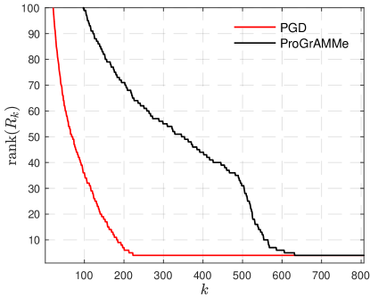
Figure 1: Rank identification of Algorithm 1.

3.2 Rank continuation

As we remarked earlier that the choice of $r$ in Algorithm 1 is crucial to its practical performance. To overcome the difficulty of a tight estimation of the rank of minimizers. In this section, we introduce a rank continuation strategy, see Algorithm 2, which adaptively adjusts the rank of the output and asymptotically attains the optimal per iteration complexity.

1:  Compute $\widetilde{W}=W\odot W,~{}L$ and et $\gamma\in]0,2/L[$; Choose $r>0$ and $I\in\mathbb{N}_{+}$;

2:  while not convergent do

3:     $Y_{k}=X_{k}+a_{k}(X_{k}-X_{k-1})$,$//$inertial step$//$     

4:     ${Z}_{k}=Y_{k}-\gamma\nabla\Psi(Y_{k})\big{(}{(\Psi(Y_{k})-F)\odot\widetilde{W}}\big{)}$,$//$gradient descent$//$     

5:     Initialize $U_{0}\in\mathbb{R}^{m\times r},V_{0}\in\mathbb{R}^{r\times n}$,

6:     for $i=1,...,I-1$ do$//$inner loop$//$     

7:       $U_{i+1}={{Z}_{k}}V_{i}^{\top}(V_{i}V_{i}^{\top}+{\tau\gamma}\mathrm{Id}_{r})^{-1}$,

8:       $V_{i+1}=(U_{i+1}^{\top}U_{i+1}+{\tau\gamma}\mathrm{Id}_{r})^{-1}U_{i+1}^{\top}{{Z}_{k}}$,

9:     end for

10:     $X_{k+1}=U_{I}V_{I}$,

11:     $r=\mathrm{rank}(U_{I})$. $//$rank continuation$//$     

12:  end while

13:  return  $X_{k+1}$

Algorithm 2 ProGrAMMe with Rank Continuation

Remark 3.3.

In Line 11, instead of using $\mathrm{rank}(X_{k+1})$ to update $r$, we choose to use $\mathrm{rank}(U_{I})$, since $\mathrm{rank}(X_{k+1})\leq\min\{\mathrm{rank}(U_{I}),\mathrm{rank}(V_{I})\}$ and it is less computational demanding to evaluate the rank of $U_{I}$ than that of $X_{k+1}$.

Remark 3.4.

Note that in Theorem 3.2, we only have rank identification property for $R_{k}$ and not for $X_{k}$. However, practically this is not an issue since we can start the rank continuation late enough such that $e_{k}$ is small enough and $\mathrm{rank}(X_{k+1})\geq\mathrm{rank}(R_{k+1})$.

Remark 3.5.

Though the initial value of $r$ is no longer as important as that of Algorithm 1 whose $r$ is fixed, it is still beneficial to have a relatively good estimate of $\mathrm{rank}(X^{\star})$ as it can further reduce the computational cost of the algorithm. Also, it is not desirable to compute $\mathrm{rank}(U_{I})$ every iteration and a practical approach is to do it every certain number of steps.

Remark 3.6.

In [46], Mazumder et al. showed that their SOFT-Impute algorithm lies in the two-dimensional maximum margin matrix factorization (MMMF) algorithm family [55]. That is, for each given maximum rank, SOFT-IMPUTE performs rank reduction and shrinkage simultaneously. However, we note that, our rank continuation strategy is different, because, we use a general weight, and perform an alternating minimization under the framework of accelerated proximal gradient.

To illustrate the performance of rank continuation, we consider a low-rank recovery problem with randomly missing entries:

$$\min_{X\in\mathbb{R}^{2000\times 2000}}{{\frac{\raisebox{0.41669pt}{\footnotesize$1$}}{\raisebox{-1.24994pt}{\footnotesize$2$}}}}\|(\Psi\odot X-F)\odot W\|^{2}+\tau\|X\|_{*},$$ (31)

where $\Psi\in\mathbb{R}^{2000\times 2000}$ is a random binary mask with $50\%$ entries equal to $0$ and

$$F=\Psi\odot\mathring{X}+\varepsilon$$

with $\mathrm{rank}(\mathring{X})=10$ and $\varepsilon$ being random Gaussian noise. For this case we set $\tau=\|\varepsilon\|$.

Comparison to SVD based PGD/FISTA.

We first compare the performances of PGD/FISTA, Algorithm 1 (ProGrAMMe) and Algorithm 2 (ProGrAMMe-RC), with the following settings:

• The step-size $\gamma$ for all these schemes are chosen as $\gamma=1/L$. Note that this choice of $\gamma$ exceeds the upper bound of step-size of FISTA, however for this example FISTA converges.

• For FISTA, we update $a_{k}$ using $a_{k}=\frac{k-1}{k+20}$ as proposed in [35] which provides faster performance than that of the standard FISTA scheme.

• For both Algorithm 1 (ProGrAMMe) and Algorithm 2 (ProGrAMMe-RC), we choose $I=1$ and $a_{k}\equiv 0$. We set $r=1,000$ for ProGrAMMe which is also the initial value of $r$ for Algorithm 2.

All schemes are stopped when the relative error $\|X_{k}-X_{k-1}\|$ reaches $10^{-10}$, and we note the the average wall clock time of $10$ runs for these schemes as:

$$\begin{matrix}\hline\cr\textrm{Schemes}&\textrm{PGD}&\textrm{FISTA}&\textrm{{ProGrAMMe}}&\textrm{{ProGrAMMe}-RC}\\ \hline\cr\textrm{Time (seconds)}&276.3&198.3&47.9&34.2\\ \hline\cr\end{matrix}$$

As illustrated in Figure 2 (a), we observe:

• PGD/FISTA is much slower than Algorithm 1 and Algorithm 2. In particular, the rank continuation scheme is about an order faster than PGD/FISTA.

• ProGrAMMe-RC is about $30\%$ faster than ProGrAMMe which indicates the advantage of rank continuation under the considered setting.

For the magenta line in Figure 2 (a) for ProGrAMMe-RC, it has several jumps which is due to the update of $r$.

(a) Comparison against PGD/FISTA

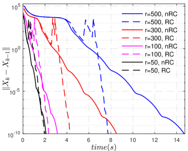
(b) Different initial values of $r$

Figure 2: Comparison of PGD/FISTA, Algorithm 1 and Algorithm 2. (a) Comparison against PGD/FISTA; (b) Comparison between rank continuation and no continuation. Note that the lines of rank continuation schemes have several jumps which is due to the update of $r$.

Effect of different starting rank.

To further understand the advantage of rank continuation over the static one, we conduct a comparison of Algorithm 2 under different initial values for $r$. Precisely, we consider

• four different values of $r=500,300,100,50$.

• $r$ is updated every $10$ steps.

We use “nRC” to denote ProGrAMMe without rank continuation and “RC” with rank continuation, and the result is shown in Figure 2 (b). We observe

• Without rank continuation, the smaller the value of $r$, the better the performance of ProGrAMMe.

• For $r=500,300$, the red and black lines in the figure, rank continuation (dashed lines) shows clear advantage over the standard scheme (solid lines).

• While for $r=100,50$, rank continuation actually becomes slower than the static scheme, and the extra time is mainly the overhead of computing $\mathrm{rank}(U_{I})$.

From the above observations, we conclude:

• For problems where a tight estimation of the rank of the solution can be obtained, one can simply consider Algorithm 1;

• When the rank of solutions is difficult to estimate, then rank continuation can be applied to achieve acceleration.

We leave the comparison of ProGrAMMe with inertial to the next section.

4 Numerical experiments

To understand the effects of inertial acceleration, validate the strengths and flexibility of our recovery model and algorithm, in this section we perform numerical experiments on several low-rank recovery problems. Throughout this section, we typically use two different versions of ProGrAMMe—(i) ProGrAMMe-$1$ which terminates the inner loop in each iteration and (ii) ProGrAMMe-$\epsilon$ which terminates the inner loop when the relative error of the inner iterates reach an $\epsilon$ precision or maximum inner iteration is achieved, whichever occurs first. Throughout the section, for ProGrAMMe-$\epsilon$, we use $\epsilon=10^{-4}$ and maximum number of inner iteration is set to 20, unless otherwise specified.

4.1 Effects of inertial acceleration

We continue the matrix completion problem (31) to study the effect of inertial acceleration. Both Algorithm 1 and 2 are tested, the setting of the tests are

• For both algorithms, we initialize $r$ with value of $500$; In terms of step-size, we keep the previous choice which is $\gamma=1/L$.

• In total, $5$ different choices of inertial parameter $a_{k}$ are considered

  $$a_{k}\equiv 0,\enskip a_{k}\equiv{{\frac{\raisebox{0.41669pt}{\footnotesize$1$}}{\raisebox{-1.24994pt}{\footnotesize$4$}}}},\enskip a_{k}\equiv{{\frac{\raisebox{0.41669pt}{\footnotesize$1$}}{\raisebox{-1.24994pt}{\footnotesize$2$}}}},\enskip a_{k}\equiv{{\frac{\raisebox{0.41669pt}{\footnotesize$3$}}{\raisebox{-1.24994pt}{\footnotesize$4$}}}}\quad\mathrm{and}\quad a_{k}={{\frac{\raisebox{0.41669pt}{\footnotesize$k-1$}}{\raisebox{-1.24994pt}{\footnotesize$k+20$}}}}.$$

The results are shown in Figure 3, whose left figure is the comparison of Algorithm 1 without rank continuation

• In general, relatively small inertial parameters ($a_{k}\equiv\frac{1}{4},\frac{1}{2}$) provide acceleration inertial schemes.

• For $a_{k}\equiv\frac{3}{4}$ and $a_{k}={{\frac{\raisebox{0.29167pt}{\footnotesize$k-1$}}{\raisebox{-0.87495pt}{\footnotesize$k+20$}}}}$ are slower than the case $a_{k}\equiv 0$.

The above observations are quite similar to the comparison of inertial schemes to proximal gradient schemes [34]. The comparison for rank continuation scheme is provided in Figure 3 (b), where similar observation as above can be obtained, except that for this case $a_{k}\equiv\frac{3}{4}$ and $a_{k}={{\frac{\raisebox{0.29167pt}{\footnotesize$k-1$}}{\raisebox{-0.87495pt}{\footnotesize$k+20$}}}}$ are faster than $a_{k}\equiv 0$.

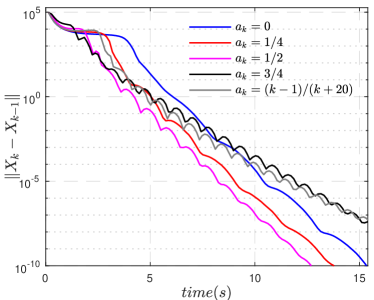
(a) No rank continuation

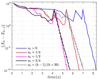
(b) Rank continuation

Figure 3: Effects of inertia: (a) No rank continuation; (b) Rank continuation.

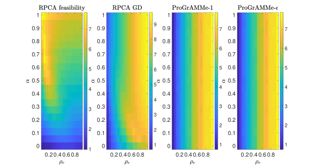
(a) Random noise

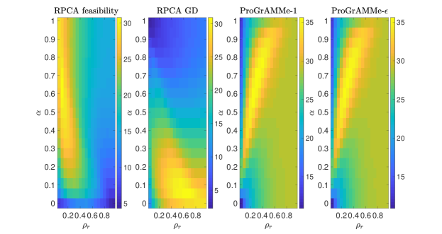
(b) Sparse large noise

Figure 4: RMSE: $\|F-X\|/\sqrt{mn}$ for different methods. Top row is for random noise, bottom row is for sparse large noise. For both cases, $\min_{i,j}W_{ij}=5,\max_{i,j}W_{ij}=10.$

4.2 Low-rank recovery experiments on synthetic data

For these experiments, we generate the low-rank matrix, $L$, as a product of two independent full-rank matrices of size $m\times r$ with $r<m$ such that elements are independent and identically distributed (i.i.d.) and sampled from a normal distribution—${\cal N}(0,1)$. We used two different types of sparse noise—Gaussian noise and arbitrary large noise. For each case, we generate the sparse matrix, $S$, such that for a sparsity level $\alpha\in(0,1)$, the sparse support is created randomly.

• For random Gaussian noise, we construct the sparse matrix $S_{\rm random}$ whose elements are i.i.d. ${\cal N}(0,1)$ random variables and form $F$ as: $F=L+\eta S_{\rm random}$, where $\eta$ controls the noise level and we set ${\eta=0.2\max_{i,j}(L)_{ij}}$.

• For large noise, we generate the sparse matrix, $S_{\rm sparse}$, such that its elements are chosen from the interval $[-50,50]$ and construct $F$ as $F=L+S_{\rm sparse}$.

We fix $m=100$, define $\rho_{r}={\rm rank}(L)/m$, where ${\rm rank}(L)$ varies and set the sparsity level $\alpha\in(0,1)$. For each $(\rho_{r},\alpha)$ pair, we apply RPCA GD [65], NCF [19], and ProGrAMMe to recover a low-rank matrix $X$. We consider RMSE, ${\|F-X\|/\sqrt{mn}}$, as performance measure.

For each class of noise, we run the experiments for 10 times and plot the average RMSEs for each $(\rho_{r},\alpha)$. Note that, RPCA GD and NCF use an operator $\mathcal{T}_{\alpha}[S]$ that does not perform an explicit Euclidean projection onto the sparse support of $S$, as the exact projection on $S$ is expensive [19, 65, 18]. Inspired by this, for sparse noise, we design our weight matrix such that it has large weights for the sparse support of $S$ and 1 otherwise. However, for random noise, we simply use a random weight matrix. From Figure 4 we see that for both random and sparse noise, ProGrAMMe has the least average RMSEs. Moreover, while two PCP algorithms show significant differences in their RMSE diagrams, our ProGrAMMe produce almost similar RMSE and obtain lower values compare to PCP algorithms in both types of noises.

Effect of the condition number of $W$ on the convergence of ProGrAMMe.

Problem (22) is tricky, as the condition number, $\kappa_{W}$ of the weight matrix, $W$ plays an important role in convergence [48, 17]. We perform a detailed empirical convergence analysis of ProGrAMMe-$\epsilon$ and ProGrAMMe-$1$ on synthetic data in Appendix A.2 by varying $\kappa_{W}$ and compared with proximal algorithms. We observe that proximal algorithms are sensitive to $\kappa_{W}$ (a higher $\kappa_{W}$, translates to a slower convergence), but both ProGrAMMe-$\epsilon$ and ProGrAMMe-$1$ are not sensitive to $\kappa_{W}$, they maintain a stable convergence profile for different $\kappa_{W}$, and converge faster than proximal algorithms in all cases. While APG takes about 0.13 seconds on an average for each experiment, ProGrAMMe-1 and ProGrAMMe-$\epsilon$ take about 0.01 seconds and 0.04 seconds, respectively.

4.3 Real-world applications

To validate the strengths and flexibility of our proposed algorithms, we use three real world problems—(i) structure from motion (SfM), (ii) matrix completion with noise, and (iii) background estimation from fully and partially observed data. We compared our algorithms against 15 state-of-the-art weighted and unweighted low-rank approximation algorithms (see Table 3 in Appendix).

Figure 5: Sample frame from the static Face, Giraffe and toy dinosaur sequences. The data matrices, $F$ are of size $2944\times 20$, $240\times 167$, and $319\times 72$, respectively and the prior rank of the sequences are 4, 6, and 4, respectively.

(i) Structure from motion and photometric stereo.

SfM uses local image features without a prior knowledge of locations or pose and infers a three dimensional structure or motion. For these experiments, we used three popular datasets: non-rigid occluded motion of a giraffe in the background (for nonrigid SfM), a toy dinosaur (for affine SfM), and the light directions and surface normal of a static face with a moving light source (for photometric stereo) (See more details in Figure 5). The datasets have 69.35%, 23.08%, and 58.28% observable entries, respectively. Therefore, we use a binary mask as weight $W$ such that $W_{ij}=1$ if the data has an entry at the $(i,j)^{\rm th}$ position, otherwise, $W_{ij}=0.$ With this setup, our formulation works as a matrix completion problem. We compared ProGrAMMe-1 and ProGrAMMe-$\epsilon$ with respect to the damped Newton algorithm in [10]. Admittedly, [10] obtains the best factorization pair, $X=UV$ such that it gives minimum loss (within the observable entry), $\frac{\|(F-X)\odot W\|}{\|W\|}$ for all cases. Additionally, we also calculated the loss outside the observable entries, that is, $\frac{\|(F-X)\odot(\mathbf{1}-W)\|}{\|\mathbf{1}-W\|}$ where the performance of ProGrAMMe is better in all cases. See results provided in Table 2 below.

Dataset	$\frac{\|(X-F)\odot W\|}{\|W\|}$	$\frac{\|(X-F)\odot(\mathbf{1}-W)\|}{\|\mathbf{1}-W\|}$
	0.5085 (ProGrAMMe-$1$)	284.1509 (ProGrAMMe-$1$)
Giraffe	0.5399 (ProGrAMMe-$\epsilon$)	271.4828 (ProGrAMMe-$\epsilon$)
	0.3228 [10]	364.2476 [10]
	4.4081 (ProGrAMMe-$1$)	244.5437 (ProGrAMMe-$1$)
Toy Dino	5.2453 (ProGrAMMe-$\epsilon$)	239.6335 (ProGrAMMe-$\epsilon$)
	1.0847 [10]	318.666 [10]
	0.023 (ProGrAMMe-$1$)	0.7143 (ProGrAMMe-$1$)
Face	0.0232 (ProGrAMMe-$\epsilon$)	0.7338 (ProGrAMMe-$\epsilon$)
	0.0223 [10]	0.98 [10]

Table 2: Comparisons between ProGrAMMe-$\epsilon$, ProGrAMMe-$1$, and damped Newton method on structure from motion and photometric stereo datasets.

(ii) Matrix completion with noise on power-grid data.

Matrix completion is one of the important special cases of weighted low-rank estimation problems as for this problem, the weights are reduced to $\{0,1\}$. This set of experiments are inspired by [15]. The dataset and the codes for BIRSVD are collected from author’s website. In this experiment, the test dataset contains 48 hours of temperature data sampled every 30 minutes over 20 European cities. The $(i,j)^{\rm th}$ entry of the matrix represents the $i^{\rm th}$ temperature measurement for the $j^{\rm th}$ city. As a prior information, we use the fact that temperature varies smoothly over time and the data matrix is low-rank.

(a) Within data

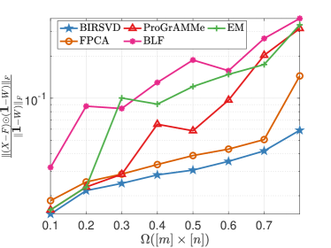
(b) Out of data

Figure 6: Fidelity within and out of the data for problem of matrix completion with noise on power-grid data. Here $\Omega$ denotes the percentage of missing data. We use ProGrAMMe-$1$ for these experiments.

For this data set, we use a rank 2 approximation. We run each algorithm with random initialization for 10 times and plot the average results in Figure 6. Each algorithm is run for 50 global iterations or tolerance set to machine precision, whichever attained first. For BIRSVD, ProGrAMMe-$1$, and BLF (with $\ell_{2}$ loss) we use $\tau=0.006$. Additionally, for BIRSVD another regularizer is set to 0 (as in [15]). FPCA [40] computes a low rank approximation by using a prior information that the nuclear norm of the matrix is bounded. As it turns out, the EM algorithm [54] has a slower convergence and the performance of ProGrAMMe is albeit better. For more discussion and detailed comparisons we refer the readers to Section A.3 in Appendix.

(iii) Background estimation.

Background estimation and moving object detection from a video sequence is a classic problem in computer vision and it plays an important role in human activity recognition, tracking, and video analysis from surveillance cameras. In the conventional matrix decomposition framework used for background estimation, the video frames are concatenated in a data matrix $F$, and the background matrix, $X$, is of low-rank [47], as the background frames are often static or close to static. However, the foreground is usually sparse. The desired target rank of the background is hard to determine due to some inherent challenges, such as, changing illumination, occlusion, dynamic foreground, reflection, and other noisy artifacts. Therefore, robust PCA algorithms such as, iEALM [36], APG [63], ReProCS [26] overcome the rank challenge robustly. However, in some cases, the target rank and the sparsity level can be part of the user-defined hyperparameters. Therefore, instead one might use a different approach as in [66, 19, 65].

For these set of experiments, we use ProGrAMMe-$\epsilon$ and compared with two different types robust PCP formulations. Note that, the PCP formulations have a way to detect the sparse outliers but our formulation does not. We overcome this challenge by using large weights. Similar to the heuristic used in the experiments for synthetic data, we choose a random subset of entries from the set $[m]\times[n]$ and use a large range of weight at those elements. This is similar to the idea used in [19, 65, 18], as for specific sparsity percentage $\alpha$, the operator $\mathcal{T}_{\alpha}[S]$ performs an approximate projection onto the sparse support of $S$. We argue that randomly selecting $\alpha\%$ of elements from ${[m]\times[n]}$ and hitting them by large weights, we obtain the same artifact. Indeed our empirical evidence in Figure 7 justifies that.

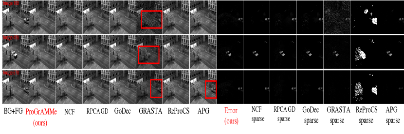
Figure 7: Sample video frames from the Stuttgart Basic video sequence. ProGrAMMe-$\epsilon$ provides a visually high quality background.

In our experiments, we use eight different video sequences: (i) the Basic sequence from Stuttgart synthetic dataset [9], (ii) four video sequences from CDNet2014 datasets [59], and (iii) three video sequences from SBI dataset [41, 1]. We extensively use the Stuttgart video sequence as it is equipped with foreground ground truth for each frame. For iEALM and APG, we set $\lambda=1/\sqrt{m}$, and use $\mu=1.25/\|F\|_{2}$ and $\rho=1.5$, where $\|F\|_{2}$ is the spectral norm (maximum singular value) of $F$. For Best pair RPCA, RPCA GD, NCF, GoDec, and our ProGrAMMe-$\epsilon$, we set $r=2$, target sparsity 10% and additionally, for GoDec, we set $q=2$. For GRATSA, we set the parameters the same as those mentioned in the authors’ website. The qualitative analysis on the background and foreground recovered suggest that our method recovers a visually similar or better quality background and foreground compare to the other methods. Note that, RPCA GD and ReProCS recover a fragmentary foreground with more false positives; moreover, GRASTA, iEALM, and APG cannot remove the static foreground object. See Section A.4 in Appendix for more qualitative results (Figure 13) and detailed quantitative results (Figure 14) of MSSIM and PSNR.

(iv) Background estimation from partially observed/missing data.

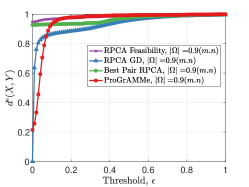
(a) $|\Omega|=0.9(m,n)$

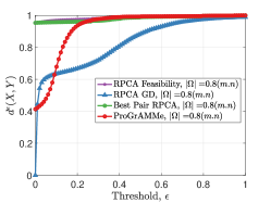
(b) $|\Omega|=0.8(m,n)$

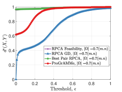
(c) $|\Omega|=0.7(m,n)$

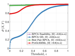
(d) $|\Omega|=0.6(m,n)$

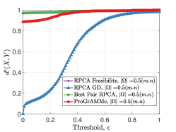
(e) $|\Omega|=0.5(m,n)$

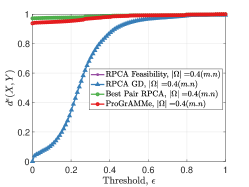
(f) $|\Omega|=0.4(m,n)$

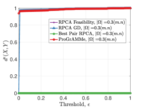
(g) $|\Omega|=0.3(m,n)$

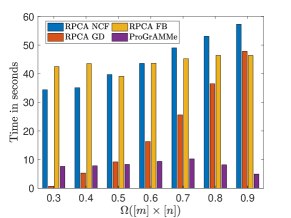
(h) Execution time

Figure 15: Quantitative comparison between different algorithms on Stuttgart Basic sequence for different levels of partially observed/missing data case with respect to the $d_{\epsilon}(X,Y)$ metric. In Figure (h), the bar diagram shows the execution time of different algorithms for different subsample $\Omega$. ProGrAMMe-$1$ has the least average execution time in all scenarios.

We randomly select the set of observable entries in the data matrix, $F$ and perform our experiments on Stuttgart Basic video. For these experiments, we use ProGrAMMe-$1$. As this is a missing data case, for ProGrAMMe-$1$, we use a binary mask as the weight. Figure 8 shows the qualitative results on different subsampled video. For a detailed quantitative evaluation of ProGrAMMe with respect to the $\epsilon$-proximity metric–$d_{\epsilon}(X,Y)$ as in [19] in recovering the foreground objects and to see the execution time for different missing data cases, see Figure 15 in Section A.5 of Appendix.

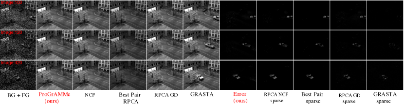
Figure 8: Sample video frames from the Stuttgart Basic video sequence for the missing data case. From top to bottom we use $\Omega=0.8,0.7,$ and 0.6, respectively.

5 Conclusions

In this paper, we proposed a generic weighted low-rank recovery model and designed an SVD-free fast algorithm for solving the model. Our model covers several existing low-rank approaches in the literature as special cases and can easily be extended to the non-convex setting. Our proposed algorithm combines proximal gradient descent method and the variational formulation of nuclear norm, which does not require to compute the SVD in each step. This makes the algorithm highly scalable to larger data and enjoys a lower per iteration complexity than those who require SVD. Moreover, based on a rank identification property, we designed a rank continuation scheme which asymptotically achieves the minimal per iteration complexity. Numerical experiments on various problems and settings were performed, from which we observe superior performance of our proposed algorithm compared to a vast class of weighted and unweighted low-rank algorithms.

Appendix A Addendum to the numerical experiments

In this section, we added some extra numerical experiments that complement our experiments and other claims in the main paper.

A.1 Table of baseline methods

In Table 3 we summarize all the methods compared in this paper.

Algorithm	Abbreviation	Appears in	Ref.
Inexact Augmented Lagrange Method of Multipliers	iEALM	Fig. 14	[36]
Proximal Gradient	PG	Fig. 9, 10	[31, 52]
Accelerated Proximal Gradient	APG	Fig. 7	[31, 52]
Accelerated Proximal Gradient-II	APG-II	Fig. 9, 10	[63]
Grassmannian Robust Adaptive Subspace Tracking Algorithm	GRASTA	Fig. 7, 8, 13, 14	[29]
Go Decomposition	GoDec	Fig. 7, 8, 13	[66]
Robust PCA Gradient Descent	RPCA GD	Fig. 4, 7, 8, 13, 14, 15	[65]
Robust PCA Nonconvex Feasibility	NCF	Fig. 4, 7, 8, 13, 15	[19]
Recursive projected compressed sensing	ReProCS	Fig. 7, 8, 13, 14	[26]
Best pair RPCA	—	Fig. 15	[18]
Fixed point Bergman	FPCA	Fig. 6, 11	[40]
Expectation Maximization	EM	Fig. 6, 11, 12	[54]
Bi-iterative regularized SVD	BIRSVD	Fig. 6, 11, 12	[15]
Bilinear factorization	BLF	Fig. 6, 11	[11]
Damped Newton	—	Table 2	[10]

Table 3: Algorithms compared in this paper.

A.2 Convergence behavior on synthetic data

In this section, we demonstrate the convergence of our algorithm(s). For this purpose, we generate the low-rank matrix, $L$, as a product of two independent full-rank matrices of size $m\times r$ with $r<m$ such that the elements are independent and identically distributed (i.i.d.) and sampled from a normal distribution—${\cal N}(0,1)$. In our setup, $m=100$, and $r=5.$ We generate $E$ as a Gaussian noise matrix whose elements are i.i.d. ${\cal N}(0,1)$ random variables and constructed $F$ as: $F=L+E$. We fixed $\min_{i,j}W_{ij}=1$, and choose $\max_{i,j}W_{ij}$ from a set $\Lambda=\{10,50,100,500,1000,5000,10^{4},5\times 10^{4},10^{5},5\times 10^{6},10^{7}\}$. At each instance, we form an $m\times m$ weight matrix, $W$ by using MATLAB function randi that generates pseudorandom integers from a uniform discrete distribution, $[\min_{i,j}W_{ij},\Lambda(p)]$, where $\Lambda(p)$ is chosen from $\Lambda$ without replacement.

We compare our ProGrAMMe-$\epsilon$ (Algorithm 1), its inexact counterpart ProGrAMMe-$1$, proximal gradient (PG) algorithm and its accelerated version—accelerated proximal gradient (APG) for these experiments. For different condition number ($\kappa_{W}$) of the weight matrix $W$, we plotted the difference between functional values evaluated at consecutive iterates, that is, $\Phi(X_{k})-\Phi(X_{k-1})$ versus iterations in Figure 9. In Figure 10, we plot the difference between consecutive iterates, $\|X_{k+1}-X_{k}\|$, versus iterations. Note that by construction, $\kappa_{W}$ ranges between 1238.021 to 21043.1574. The convergence plots justify our claims, that, although problem (5) belongs to the class of problems (8), the general algorithms used in [31, 52, 57, 38] fail to provide good convergence results when $\kappa_{W}$ is large; that, our approaches are faster compare to those general approaches; and, that the performance of both exact and inexact ProGrAMMe are the same. Moreover, in all cases, ProGrAMMe-$\epsilon$ and ProGrAMMe-$1$ can recover the rank 5 low-rank matrix, but PG and APG mostly recover a full-rank matrix. We hypothesize this is due to the sensitivity of PG and APG algorithms on the balancing parameter, $\tau$ which is required to perform the proximal mapping (in this case, the singular value thresholding [12, 27]); see also Figure 2.

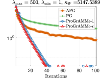
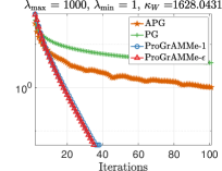
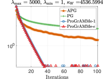
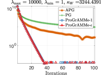
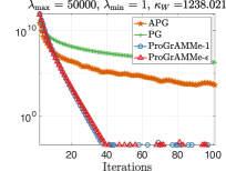
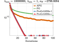
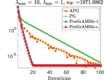
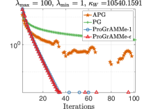
Figure 9: Convergence in terms of functional values evaluated at consecutive iterates, that is, $\Phi(X_{k})-\Phi(X_{k-1})$ vs. iterations of proximal gradient (5) (Direct PG), accelerated proximal gradient-II (APG-II), ProGrAMMe-$1$, and ProGrAMMe-$\epsilon$ applied to original problem. Note that, $\Phi(X)=f(X)+g(X)$; see details in Section 2.1. We set $\tau=10^{-2}/{\lambda^{2}_{\max}}$.

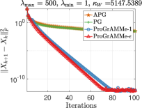
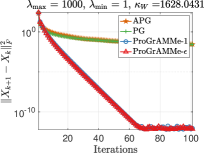
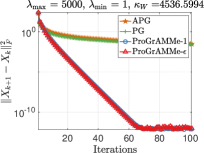
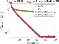
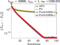
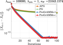
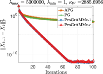
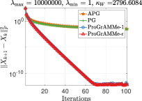
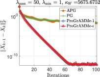
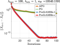
Figure 10: Convergence in terms of difference between consecutive iterates ($\|X_{k+1}-X_{k}\|$) vs. of proximal gradient (5) (Direct PG), accelerated proximal gradient-II (APG-II), ProGrAMMe-$\epsilon$ (Algorithm 1), and ProGrAMMe-$1$ applied to original problem. We set $\tau=10^{-2}/{\lambda^{2}_{\max}}$.

A.3 Matrix completion with missing data—Effect of more global iterations

In this part, we conduct extensive tests of the power-grid missing data problem. For first set of experiments, we ran the methods until the relative error, $\|X_{k+1}-X_{k}\|/\|X_{k}\|$ or consecutive iteration error, $\|X_{k+1}-X_{k}\|$ is less than the machine precision or a maximum number of iterations (500) is reached, whichever happens first. Eventually, Figure 11 shows that the performance of ProGrAMMe-$1$ improves as it runs for more global iterations although it has a fractions of the execution time compare to the other methods. Next, in Figure 12 we ran more samples (50) with the same stopping criteria as before but with an increased number of iterations (1000). From Figure 12 we find that for fidelity inside the sample, ProGrAMMe-$1$ performs better than the two previously best performing methods—EM and BIRSVD. Nevertheless, for fidelity outside the sample BIRSVD is still the best, but the behavior of ProGrAMMe improves compared to the previous cases.

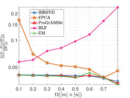
(a) Fidelity within data

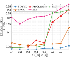
(b) Fidelity out of data

(c) Execution time

Figure 11: Fidelity within and out of the data, ran for more number of iterations (500). Here $\Omega$ denotes the percentage of missing data. The last bar diagram shows the execution time of different algorithms for different subsample $\Omega$. Although BLF with $\ell_{2}$ loss has the least execution time, its performance is not so good for this set of experiments.

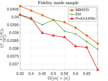
(a) Fidelity within the sample

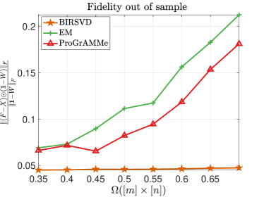
(b) Fidelity out of the sample

Figure 12: Fidelity within and out of the sample, ran for more samples (50) over a higher number of iterations (1000). Here $\Omega$ denotes the percentage of missing data.

Figure 13: Sample video frames from the CDNet 2014 and SBI dadasets. ProGrAMMe provides a visually high quality background for almost all sequences. The red bounding boxes in recovered BG denote shadows, ghosting effects of FG objects, static FG object etc.

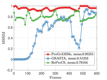
(a) Mean SSIM

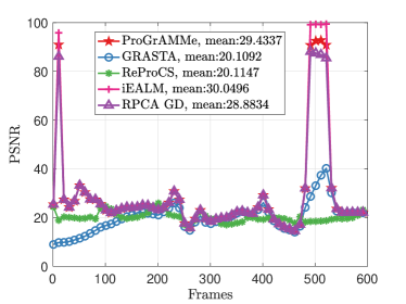
(b) PSNR

Figure 14: Quantitative comparison of different algorithms on Stuttgart Basic sequence. We compare the recovered foreground by different methods with respect to the foreground GT available for each frame on two different metrics: mean SSIM and PSNR.

A.4 Background estimation–Additional qualitative and quantitative evaluation

We show the qualitative results on 7 other real-world video sequences from the CDNet 2014 and SBI datasets in Figure 13. In almost all sequences, ProGrAMMe-$\epsilon$ performs consistently well compare to the other state-of-the-art methods. We do not include iEALM or APG due to their higher execution time.

In Figure 14, we show two robust quantitative measures for the background estimation experiments on Stuttgart Basic video: peak signal to noise ratio (PSNR) and mean structural similarities index measure (SSIM) [60]. PSNR is defined as $10\log_{10}$ of the ratio of the peak signal energy to the mean square error (MSE) between the processed video signal and the ground truth. Let $F(:,i)-\hat{X}(:,i)$ be the reconstructed vectorized foreground frame and $G(:,i)$ be the corresponding ground truth frame, then PSNR is defined as $10\log_{10}\frac{{\rm M}_{I}^{2}}{{\rm MSE}}$, where ${\rm MSE}=\frac{1}{mn}\|F(:,i)-\hat{X}(:,i)-G(:,i)\|^{2}$ and ${\rm M}_{I}=255$ is the maximum possible pixel value of the image, as the pixels are represented using 8 bits per sample. For a reconstructed image with 8 bits bit depth, the PSNR are between 30 and 50 dB, where the higher is the better as we minimize the MSE between images with respect the maximum signal value of the image.

For both measures, we perceive the information how the high-intensity regions of the image are coming through the noise, and pay less attention to the low-intensity regions. We remove the noisy components from the recovered foreground, $F(:,i)-\hat{X}(:,i)$, by using the threshold $\epsilon^{\prime}$, such that we set the components below $\epsilon^{\prime}$ in $E$ to 0. In our experiments, we set $\epsilon^{\prime}=10^{-4}$. To calculate the SSIM of each recovered foreground video frame, we consider an $11\times 11$ Gaussian window with standard deviation ($\sigma$) 1.5 and consider the corresponding ground truth as the reference image. Among the methods tested, ProGrAMMe-$\epsilon$ has the highest average SSIM (or MSSIM). To compare PSNR of recovered foreground frames, we use ProGrAMMe-$\epsilon$, GRASTA [29], recursive projected compressive sensing (ReProCS)[26], inexact ALM (iEALM) [36], and RPCA GD [65]. iEALM has the highest average PSNR, 30.05 dB among all the methods, whereas ProGrAMMe-$\epsilon$ has albeit less, an average PSNR 29.45 dB. However, ProGrAMMe-$\epsilon$ needs an average 9.48 seconds to produce the results, compared to the average execution time of iEALM is 183 seconds.

A.5 Background estimation from partially observed/missing data—Quantitative evaluation

For background estimation on partially observed data we used the $\epsilon$-proximity metric—$d_{\epsilon}(X,Y)$ proposed in [19] on Stuttgart Basic video. The performance of RPCA nonconvex feasibility (RPCA feasibility or RPCA NCF) [19] with respect to $d_{\epsilon}(X,Y)$ stays stable for all subsample $\Omega$. The performance of the best pair RPCA (also known as RPCA forward-backward or RPCA FB) [18] is stable except for $\Omega=0.3$. The performance of RPCA GD [65] keeps downgrading as we decrease the cardinality of the support $\Omega$. Surprisingly, the performance of ProGrAMMe-$1$ gets better for this experiment as we decrease $\Omega$. Furthermore, the average execution time for ProGrAMMe-$1$ is stable for different $\Omega$, and is around 8 seconds. While the next best average execution time 19.67 seconds is recorded for RPCA GD. The average execution time of NCF and best pair are 44 and 43 seconds, respectively.

Acknowledgement

Aritra Dutta acknowledges being an affiliated researcher at the Pioneer Centre for AI, Denmark. Jingwei Liang acknowledges support from the Shanghai Municipal Science and Technology Major Project (2021SHZDZX0102) and the support from SJTU and Huawei ExploreX Funding (SD6040004/033).

References

- [1] http://sbmi2015.na.icar.cnr.it/SBIdataset.html.
- [2] H. Attouch, J. Bolte, P. Redont, and A. Soubeyran. Proximal alternating minimization and projection methods for nonconvex problems: An approach based on the kurdyka-łojasiewicz inequality. Mathematics of operations research, 35(2):438–457, 2010.
- [3] H. Attouch, J. Bolte, and B. F. Svaiter. Convergence of descent methods for semi-algebraic and tame problems: proximal algorithms, forward–backward splitting, and regularized Gauss–Seidel methods. Mathematical Programming, 137(1-2):91–129, 2013.
- [4] J.-F. Aujol and C. Dossal. Stability of over-relaxations for the forward-backward algorithm, application to fista. SIAM Journal on Optimization, 25(4):2408–2433, 2015.
- [5] J. B. Baillon and G. Haddad. Quelques propriétés des opérateurs angle-bornés etn-cycliquement monotones. Israel Journal of Mathematics, 26(2):137–150, 1977.
- [6] A. Beck and M. Teboulle. A fast iterative shrinkage-thresholding algorithm for linear inverse problems. SIAM Journal on Imaging Science, 2(1):183–202, 2009.
- [7] T. Boas, A. Dutta, X. Li, K. P. Mercier, and E. Niderman. Shrinkage function and its applications in matrix approximation. Electronic Journal of Linear Algebra, 32:163–171, 2017.
- [8] J. Bolte, S. Sabach, and M. Teboulle. Proximal alternating linearized minimization for nonconvex and nonsmooth problems. Mathematical Programming, 146(1-2):459–494, 2014.
- [9] S. Brutzer, B. Hoferlin, and G. Heidemann. Evaluation of background subtraction techniques for video surveillance. In IEEE Computer Vision and Pattern Recognition, pages 1937–1944, 2011.
- [10] A. M. Buchanan and A. W. Fitzgibbon. Damped Newton algorithms for matrix factorization with missing data. In IEEE Computer Vision and Pattern Recognition, volume 2, pages 316–322, 2005.
- [11] R. Cabral, F. D. L. Torre, J. P. Costeira, and A. Bernardino. Unifying nuclear norm and bilinear factorization approaches for low-rank matrix decomposition. In 2013 IEEE International Conference on Computer Vision, pages 2488–2495, 2013.
- [12] J. F. Cai, E. J. Candès, and Z. Shen. A singular value thresholding algorithm for matrix completion. SIAM Journal on Optimization, 20(4):1956–1982, 2010.
- [13] E. J. Candès and B. Recht. Exact matrix completion via convex optimization. Foundations of Computational Mathematics, 9(6):717–772, 2009.
- [14] A. Chambolle and C. Dossal. On the convergence of the iterates of the “fast iterative shrinkage/thresholding algorithm”. Journal of Optimization Theory and Applications, 166(3):968–982, 2015.
- [15] S. Das and A. Neumaier. Regularized low rank approximation of weighted data sets, 2011.
- [16] A. Dutta. Weighted Low-Rank Approximation of Matrices:Some Analytical and Numerical Aspects. PhD thesis, University of Central Florida, 2016.
- [17] A. Dutta, B. Gong, X. Li, and M. Shah. Weighted singular value thresholding and its application to background estimation, 2017. arXiv:1707.00133.
- [18] A. Dutta, F. Hanzely, J. Liang, and P. Richtárik. Best pair formulation & accelerated scheme for non-convex principal component pursuit. IEEE Transactions on Signal Processing, 68:6128–6141, 2020.
- [19] A. Dutta, F. Hanzely, and P. Richtárik. A nonconvex projection method for robust PCA. In Thirty-Third AAAI Conference on Artificial Intelligence (AAAI-19), pages 1468–1476, 2018.
- [20] A. Dutta and X. Li. A fast algorithm for a weighted low rank approximation. In 15th IAPR International Conference on Machine Vision Applications (MVA), pages 93–96, 2017.
- [21] A. Dutta and X. Li. On a problem of weighted low-rank approximation of matrices. SIAM Journal on Matrix Analysis and Applications, 38(2):530–553, 2017.
- [22] A. Dutta and X. Li. Weighted low rank approximation for background estimation problems. In The IEEE International Conference on Computer Vision Workshops (ICCVW), pages 1853–1861, 2017.
- [23] A. Dutta, X. Li, and P. Richtárik. Weighted low-rank approximation of matrices and background modeling, 2018. arXiv:1804.06252.
- [24] C. Eckart and G. Young. The approximation of one matrix by another of lower rank. Psychometrika, 1(3):211–218, 1936.
- [25] E. Grave, G. R Obozinski, and F. R Bach. Trace lasso: a trace norm regularization for correlated designs. In Advances in Neural Information Processing Systems, pages 2187–2195, 2011.
- [26] H. Guo, C. Qiu, and N. Vaswani. An online algorithm for separating sparse and low-dimensional signal sequences from their sum. IEEE Transactions on Signal Processing, 62(16):4284–4297, 2014.
- [27] E.T. Hale, W. Yin, and Y. Zhang. Fixed-point continuation for -minimization: methodology and convergence. SIAM Journal on Optimization, 19:1107–1130, 2008.
- [28] W. L. Hare and A. S. Lewis. Identifying active constraints via partial smoothness and prox-regularity. Journal of Convex Analysis, 11(2):251–266, 2004.
- [29] J. He, L. Balzano, and A. Szlam. Incremental gradient on the Grassmannian for online foreground and background separation in subsampled video. IEEE Computer Vision and Pattern Recognition, pages 1937–1944, 2012.
- [30] M. Jaggi, M. Sulovsk, et al. A simple algorithm for nuclear norm regularized problems. In Proceedings of the 27th international conference on machine learning (ICML-10), pages 471–478, 2010.
- [31] S. Ji and J. Ye. An accelerated gradient method for trace norm minimization. In Proceedings of the 26th Annual International Conference on Machine Learning, pages 457–464, 2009.
- [32] I. T. Jolliffee. Principal component analysis. Springer-Verlag, second edition, 2002.
- [33] A. S. Lewis. Active sets, nonsmoothness, and sensitivity. SIAM Journal on Optimization, 13(3):702–725, 2003.
- [34] J. Liang, J. Fadili, and G. Peyré. Activity identification and local linear convergence of forward–backward-type methods. SIAM Journal on Optimization, 27(1):408–437, 2017.
- [35] J. Liang, T. Luo, and C. Schönlieb. Improving fista: Faster, smarter and greedier. arXiv preprint arXiv:1811.01430, 2018.
- [36] Z. Lin, M. Chen, and Y. Ma. The augmented Lagrange multiplier method for exact recovery of corrupted low-rank matrices, 2010. arXiv1009.5055.
- [37] P. L. Lions and B. Mercier. Splitting algorithms for the sum of two nonlinear operators. SIAM Journal on Numerical Analysis, 16(6):964–979, 1979.
- [38] Y. Liu, H. Cheng, F. Shang, and J. Cheng. Nuclear norm regularized least squares optimization on grassmannian manifolds. In Proceedings of the Thirtieth Conference on Uncertainty in Artificial Intelligence, UAI’14, pages 515–524, 2014.
- [39] W. S. Lu, S. C. Pei, and P. H. Wang. Weighted low-rank approximation of general complex matrices and its application in the design of 2-d digital filters. IEEE Transactions on Circuits and Systems I: Fundamental Theory and Applications, 44(7):650–655, 1997.
- [40] S. Ma, D. Goldfarb, and L. Chen. Fixed point and bregman iterative methods for matrix rank minimization. Mathematical Programming, 128(1-2):321–353, 2011.
- [41] L. Maddalena and A. Petrosino. Towards benchmarking scene background initialization. In New Trends in Image Analysis and Processing – ICIAP 2015 Workshops, pages 469–476, 2015.
- [42] J. H. Manton, R. Mehony, and Y. Hua. The geometry of weighted low-rank approximations. IEEE Transactions on Signal Processing, 51(2):500–514, 2003.
- [43] I. Markovsky. Low-rank approximation: algorithms, implementation, applications, 2012. Springer.
- [44] I. Markovsky, J. C. Willems, B. De Moor, and S. Van Huffel. Exact and approximate modeling of linear systems: a behavioral approach, Number 11 in Monographs on Mathematical Modeling and Computation. SIAM, 2006.
- [45] G. Mateos and G. Giannakis. Robust PCA as bilinear decomposition with outlier-sparsity regularization. IEEE Transaction on Signal Processing, 60(10):5176–5190, 2012.
- [46] Rahul Mazumder, Trevor Hastie, and Robert Tibshirani. Spectral regularization algorithms for learning large incomplete matrices. Journal of Machine Learning Research, 11(80):2287–2322, 2010.
- [47] N. Oliver, B. Rosario, and A. Pentland. A Bayesian computer vision system for modeling human interactions. In International Conference on Computer Vision Systems, pages 255–272, 1999.
- [48] T. Pong, P. Tseng, S. Ji, and J. Ye. Trace norm regularization: Reformulations, algorithms, and multi-task learning. SIAM J. on Optimization, 20(6):3465–3489, 2010.
- [49] I. Razenshteyn, Z. Song, and D. P. Woodruff. Weighted low rank approximations with provable guarantees. In Proceedings of the forty-eighth annual ACM symposium on Theory of Computing, pages 250–263. ACM, 2016.
- [50] B. Recht, M. Fazel, and P. Parrilo. Guaranteed minimum-rank solutions of linear matrix equations via nuclear norm minimization. SIAM Review, 52(3):471–501, 2010.
- [51] J. D. M. Rennie and N. Srebro. Fast maximum margin matrix factorization for collaborative prediction. In Proceedings of the 22Nd International Conference on Machine Learning, ICML ’05, pages 713–719, 2005.
- [52] Z. Shen, K. Toh, and S. Yun. An accelerated proximal gradient algorithm for nuclear norm regularized linear least squares problems. Pacific J. Optim, pages 615–640, 2009.
- [53] D. Shpak. A weighted-least-squares matrix decomposition with application to the design of 2-d digital filters. Proceedings of IEEE 33rd Midwest Symposium on Circuits and Systems, pages 1070–1073, 1990.
- [54] N. Srebro and T. Jaakkola. Weighted low-rank approximations. 20th International Conference on Machine Learning, pages 720–727, 2003.
- [55] Nathan Srebro, Jason Rennie, and Tommi Jaakkola. Maximum-margin matrix factorization. In Advances in Neural Information Processing Systems, volume 17, 2004.
- [56] M. Tao and J. Yang. Recovering low-rank and sparse components of matrices from incomplete and noisy observations. SIAM Journal on Optimization, 21(1):57–81, 2011.
- [57] K. Toh and S. Yun. An accelerated proximal gradient algorithm for nuclear norm regularized least squares problems. 2009.
- [58] K. Usevich and I. Markovsky. Variable projection methods for affinely structured low-rank approximation in weighted 2-norms. Journal of Computational and Applied Mathematics, 272:430–448, 2014.
- [59] Y. Wang, P.-M. Jodoin, F. Porikli, J. Konrad, Y. Benezeth, and P. Ishwar. Cdnet 2014: an expanded change detection benchmark dataset. In Proceedings of the IEEE conference on computer vision and pattern recognition workshops, pages 387–394, 2014.
- [60] Z. Wang, A. C. Bovik, H. R. Sheikh, and E. P. Simoncelli. Image quality assessment: from error visibility to structural similarity. IEEE Transaction on Image Processing, 13(4):600–612, 2004.
- [61] F. Wen, R. Ying, P. Liu, and T.-K. Truong. Nonconvex regularized robust pca using the proximal block coordinate descent algorithm. IEEE Transactions on Signal Processing, 67(20):5402–5416, 2019.
- [62] Z. Wen, W. Yin, and Y. Zhang. Solving a low-rank factorization model for matrix completion by a nonlinear successive over-relaxation algorithm. Mathematical Programming Computation, 4(4):333–361, 2012.
- [63] J. Wright, Y. Peng, Y. Ma, A. Ganseh, and S. Rao. Robust principal component analysis: exact recovery of corrputed low-rank matrices by convex optimization. Proceedings of 22nd Advances in Neural Information Processing systems, pages 2080–2088, 2009.
- [64] Y. Xiao, L. Li, T. Yang, and L. Zhang. Svd-free convex-concave approaches for nuclear norm regularization. In Proceedings of the Twenty-Sixth International Joint Conference on Artificial Intelligence, IJCAI-17, pages 3126–3132, 2017.
- [65] X. Yi, D. Park, Y. Chen, and C. Caramanis. Fast algorithms for robust PCA via gradient descent. Advances in Neural Information Processing systems, pages 361–369, 2016.
- [66] T. Zhou and D. Tao. Godec: Randomized low-rank and sparse matrix decomposition in noisy case. In Proceedings of the 28th International Conference on Machine Learning (ICML), pages 33–40, 2011.