Bankruptcy prediction using disclosure text features

Abstract

A public firm’s bankruptcy prediction is an important financial research problem because of the security price downside risks. Traditional methods rely on accounting metrics that suffer from shortcomings like window dressing and retrospective focus. While disclosure text-based metrics overcome some of these issues, current methods excessively focus on disclosure tone and sentiment. There is a requirement to relate meaningful signals in the disclosure text to financial outcomes and quantify the disclosure text data. This work proposes a new distress dictionary based on the sentences used by managers in explaining financial status. It demonstrates the significant differences in linguistic features between bankrupt and non-bankrupt firms. Further, using a large sample of 500 bankrupt firms, it builds predictive models and compares the performance against two dictionaries used in financial text analysis. This research shows that the proposed stress dictionary captures unique information from disclosures and the predictive models based on its features have the highest accuracy.

Keywords Bankruptcy  $\cdot$ Distress  $\cdot$ NLP  $\cdot$ bag-of-words  $\cdot$ Disclosures  $\cdot$ Machine learning  $\cdot$ EDGAR  $\cdot$ Text analysis  $\cdot$ 10-K

1 Introduction

Investors and analysts place great emphasis on security analysis and valuation because of the potential excess returns on capital and the downside risks. Research in this domain is potentially valuable because market inefficiencies can result in volatility and crashes, costing the economy billions of dollars. Analysts extensively use public firm’s disclosures as a source of information.

Investors are keen on knowing about the health of the firms they may invest in the future. A firm in financial distress loses a significant amount of its shareholder’s value. If the management cannot tide over the crisis, the firm may have to file for bankruptcy, resulting in a 50% to 80% loss of capital for shareholders and lenders. Financial distress and bankruptcy prediction is an actively researched field.

Once a company is unable to come out of distress, it will become insolvent. Insolvency is the state in which the company is not capable of honoring some commitment. Lenders and claim holders can force the insolvent company to discontinue operations. Managements file for bankruptcy protection to recover from such a situation or liquidate it in an orderly manner. Bankruptcy prediction has been an active research topic for accounting researchers over decades. One of the pioneering works Altman (1968) proposed the ‘Z score’ model.

Investors and analysts traditionally depended on quantitative information like accounting metrics for decision making. Multiple attributes of these accounting metrics drove this trend. FACC and accounting standards laid out what variables to be measured and disclosed. Gathering, processing, and analyzing these quantitative metrics was easy. Many free and commercial data providers automated the data gathering and published these metrics. However, these metrics do not always reveal the firm’s current status and are not a good indicator of the future. They suffer from shortcomings like window dressing and retrospective focus.

Evidence exists for window dressing through commissions and omissions. Rajan, Seru, and Vig (2015) showed that banks did not report information regarding the deteriorating quality of borrowers’ disclosures in the run-up to the subprime crisis. Huizinga and Laeven (2012) said that banks overstated the value of their distressed real estate assets and regulatory capital. Window dressing, retrospective focus, and missing variables impact models based on accounting metrics. Regulators and investors who rely on such models have been impacted adversely in the past due to model failures (Rajan, Seru, and Vig (2015)).

Another approach for bankruptcy prediction is using market-based information. Classical efficient market theory and later option pricing theories assume that all available information is reflected in market prices. Under those conditions, accounting-based metrics do not have additional information over and above market prices. More specifically, a suitable market-based measure will reflect all available information about bankruptcy probability. Hillegeist et al. (2004) developed a prediction model based on market information, using option pricing theory derived implied volatility. This model outperformed the Altman (1968) z score model. Subsequently, numerous attempts have been made to replicate these results. Wu, Gaunt, and Gray (2010) provides a comparison of accounting and market-based models, along with others. They conclude that the Hillegeist et al. (2004) model performs better than the Z score model but is inferior to models that include non-traditional metrics. Similarly, Tinoco and Wilson (2013) concluded that accounting metrics based models and market-based models are complimentary.

Hence researchers started paying more attention to alternative approaches like textual analysis of disclosures. Management disclosures have narrative content that contains important information. This information can explain many firm attributes and organization outcomes, and text analysis methods can extract this information. Prior works have attempted to incorporate text features into accounting-based predictive models. However, standalone text feature-based prediction models have not been attempted. There is a need to understand how much information can be extracted from disclosure texts and how useful, such information is in predicting bankruptcy. This work addresses that gap.

2 Related work

Numerous researchers tried to explain various firm attributes using disclosure narratives. Some analyzed MDA to explain future stock performance (Tao, Deokar, and Deshmukh (2018)), future returns, volatility, and firm profitability (Amel-Zadeh and Faasse (2016)), bankruptcy (Yang, Dolar, and Mo (2018)), going-concern (Mayew, Sethuraman, and Venkatachalam (2015),Enev (2017)), litigation risk (Bourveau, Lou, and Wang (2018)), and incremental information over earnings surprises, accruals and operating cash flows (OCF)(Feldman et al. (2008),Feldman et al. (2010)).

Researchers attempted to incorporate text features into distress and bankruptcy predictive models. Below is a brief review of the same.

Auditors express going-concern opinions based on the firm’s obligations and liquidity. Financial disclosures include these opinions. Change in such disclosures can act as a signal to identify distress. However, auditors do respond to external financial markets. Beams and Yan (2015) examined the financial crisis’s effect on auditor going-concern opinions and concluded that the financial crisis led to increased auditor conservatism. A going-concern opinion in disclosures is associated with the number of forward-looking disclosures and their ambiguity. Enev (2017) observed that while the absolute number of forward-looking disclosures is lower for companies receiving a going concern opinion, the proportion of forward-looking disclosures in the MDA is higher in the presence of a going concern opinion. The results suggest generally improved forward-looking disclosures in MDA when companies receive a going concern opinion from their auditor.

One consequence of distress is financial constraints. Firms undergo reduced cash flows during Stress, which results in liquidity events - like dividend omissions or increases, equity recycling, and underfunded pensions. Analysts measure the extent of financial constraints to assess the capital structure. Bodnaruk, Loughran, and McDonald (2013) used a constraining-words-based lexicon to measure the same. These measures have a low correlation with traditional financial constraints measures and predict subsequent liquidity events better. Ball, Hoberg, and Maksimovic (2012) used text in firms’ 10-Ks to measure investment delays due to financial constraints. They found that the fundamental limitations are the financing of R&D expenditures rather than capital expenditures and that the main challenge for firms is raising equity capital to fund growth opportunities. These text-based measures predict investment cuts following the financial crisis better than other indices of financial constraints used in the literature.

Most prior bankruptcy prediction models were developed by using financial ratios. However, signs of distress may appear in the nonfinancial information earlier than changes in the financial ratios. Current distress measures tend to miss extreme events, especially in the banking sector (Gandhi, Loughran, and McDonald (2017)). In recent years, qualitative information and text analysis have become necessary because frequent changes in accounting standards have made it difficult to compare financial numbers between years (Shirata et al. (2011)). Mayew, Sethuraman, and Venkatachalam (2015) stressed the importance of linguistic tone in assessing a firm’s health. Using a sample of bankrupt firms between 1995 and 2012, they concluded that management’s opinion about going-concern and the MDA’s linguistic tone together predict whether a firm will go bankrupt.

The language used by future bankrupt companies differs from non-bankrupt companies. Hájek and Olej (2015) studied various word categories from corporate annual reports and showed that the language used by bankrupt companies shows stronger tenacity, accomplishment, familiarity, present concern, exclusion, and denial. Bankrupt companies also use more modal, positive, uncertain, and negative language. They built prediction models combining both financial indicators and word categorizations as input variables. This differential language usage is observed in non-English firms’ disclosures also. Shirata et al. (2011) analyzed the sentences in Japanese financial reports to predict bankruptcy. Their research revealed that the co-occurrence of words “dividend” or “retained earnings” in a section distinguish between bankrupt companies and non-bankrupt companies.

Working on U.S. Banks Gandhi, Loughran, and McDonald (2017) used disclosure text sentiment as a proxy for bank distress. They found that the annual report’s more negative sentiment is associated with larger delisting probabilities, lower odds of paying subsequent dividends, higher subsequent loan loss provisions, and lower future return on assets. Similarly, Lopatta, Gloger, and Jaeschke (2017) concluded that firms at risk of bankruptcy use significantly more negative words in their 10-K filings than comparable vital companies. This relationship holds up until three years before the actual bankruptcy filing. Other notable works using text analysis for bankruptcy prediction were Yang, Dolar, and Mo (2018) and Mayew, Sethuraman, and Venkatachalam (2015). Yang, Dolar, and Mo (2018) used high-frequency words from MDA and compared the differences between bankrupt and non-bankrupt companies. Mayew, Sethuraman, and Venkatachalam (2015) also analyzed MDA with a focus on going-concern options. They found that both management’s opinion about “going-concern” reported in the MDA and the MDA’s linguistic tone together provide significant explanatory power in predicting whether a firm will cease as a going concern. Also, the predictive ability of disclosure is incremental to financial ratios, market-based variables, even the auditor’s going concern opinion and extends to three years before the bankruptcy.

Most of the prior works focused on disclosure sentiment as an incremental predictor for bankruptcy prediction. However, disclosure text contains significantly more information other than sentiment, and there is a need to extract and test its predictive power. To this end, this quantitative correlation study evaluates the differences in linguistic features between healthy and bankrupt disclosure texts. Further, predictive models are built to assess the information content and predictive power. The next section will outline the methods.

3 Method and materials

The prior sections have reviewed the literature and identified the gaps in the text analysis of finance. As bankruptcy is a significant organizational outcome for investors, this thesis focuses on the bankruptcy prediction task. To this end, this quantitative correlation study evaluates the differences in linguistic features between healthy and bankrupt disclosure texts. Further, predictive models are built to assess the information content and predictive power. This section describes the framework, data analysis, and methodology used.

To summarize, this thesis has four key components.

Text source: Management Discussion and Analysis from 10-K disclosures.
Task: Bankruptcy prediction based on prior-year MDA.
Sample size: Balanced sample with 500 number of bankrupt and non-bankrupt disclosures each.
Language models: Multiple, as described in later parts of this chapter.

The methods section consists of 4 sub-sections covering data, language models, predictive models, and assessment criteria.

3.1 Sample selection criteria and data sources

In this section, sample selection and data collection methods are described. This work aims to extract knowledge from financial disclosure text and use it for predictive tasks. It considers public listed companies in the U.S. as the population. From 1994 to 2019, over 16,000 individual companies filed annual disclosures with SEC. New companies get listed on exchanges through Initial Public Offering or corporate spin-offs. Companies are delisted due to mergers, acquisitions, and bankruptcies. As a result, there are ~8000 listed public companies in the year 2019 in the U.S.

This work focuses on bankruptcy prediction using disclosure text characteristics. So, two samples are critical. One is a list of bankrupt firms, and the other is a list of non-bankrupt firms.

3.1.1 Bankrupt firms

A critical component of this study is to identify firms that went bankrupt. This work uses the list of bankrupt companies from the UCLA-LoPucki Bankruptcy Research Database (BRD) maintained by LoPucki (2006). UCLA School of Law collects, updates, and disseminates this data. This dataset contains more than one-thousand large public companies that have filed bankruptcy cases since October 1, 1979. BRD defines a public company as a firm that filed an Annual Report (Form 10-K or form 10) with the SEC for a year ending not less than three years before filing the bankruptcy case. BRD considers all firms with more than $ 100 million in assets in annual reports as “large.” Assets are measured in 1980 constant dollars (about $ 3.1 current dollar). Both Chapter 7 and Chapter 11 cases are included in the bankruptcy list, whether filed by the debtors or creditors. From this list, bankruptcies before 1994 are excluded. Since EDGAR maintains online disclosures from 1994 onwards, it was convenient to extract those filings. The exclusion of prior bankruptcies results in a new list of ~900 bankrupt companies. Around 7000 corresponding firm filings exist in EDGAR. Companies without at least one prior year 10-K filing are excluded from the list. Finally, the Management Discussion and Analysis sections are extracted from these filings. A minimum threshold of 100 words is used to filter out non-informative MDAs. This filtering resulted in a sample of 500 company filings one year before bankruptcy.

3.1.2 Non-Bankrupt firms

List of Non-Bankrupt firms is identified by starting with S&P 1000 list and excluding companies with bankruptcy history. The net result is 980 firms. Around 16000 filings exist for all these firms.

3.1.3 Sample size

Since annual bankruptcy incidence is less than 0.5%, the number of all filings one year prior to bankruptcies is very low, compared to non-bankrupt filings. Hence, a balanced experiment design with an equal number of bankrupt and non-bankrupt disclosures in the sample is used. Five hundred non-bankrupt filings are randomly chosen from the non-bankrupt filings.

3.2 Data collection

The method for the annual filings downloading has the below components.

3.2.1 SEC data extraction

From 1993 to 2018, Dec companies filed ~20 million records on EDGAR. For ease of access, SEC releases quarterly master indices for the list of filings on EDGAR. This list has ~ 220,00 annual (10-K) filings relevant to this thesis. Custom R and python scripts downloaded these 10-K documents programmatically.

3.2.2 Data cleaning

The text version of the filings on SEC is a collection of all files in a submission. These include HTML, exhibits, jpg files, and XBRL files. A fraction of the text file size will contain actual text. ASCII-encoded pdfs, graphics, Xls, or other binary files can contribute to most of the filings document size. The next processing step removed all non-text content from disclosure documents, following Loughran and Mcdonald (2009). These cleaned filings are stored in text format.

3.2.3 MDA extraction

For bankruptcy prediction, Management Analysis, and Discussion (MDA) is the text features source. Management teams discussed the current firm status and expected outcomes in the MDA section. A python script extracted all the text between “ITEM 7” and “ITEM 7 A”. Regular expressions and combinations of these phrases are used to identify the maximum number of the MDAs from 10-K files. In some disclosures, the MDA section is “incorporated by reference,” referring to the shareholder’s annual report. The thesis included MDA material from the body of the primary document. Also, it discarded all MDAs with less than a 100-word count. Subsequent sections explain the generation of these texts’ numeric representation by using dictionary-based parsing or word embeddings.

3.3 Variable selection and language models

This subsection explains the dependent and independent variables used in the thesis.

3.3.1 Outcome definition

The dependent variable for this thesis is a Bankruptcy filing. The Bankruptcy filing Dummy equals one if the firm has filed for bankruptcy protection within one year after the 10-K filing date, else 0.

3.3.2 Independent variable selection

As outlined in the prior literature survey, numerous text representation methods successfully extract information from financial disclosures. However, often, they were used in combination with traditional quantitative metrics and financial ratios. This thesis aims to identify standalone information content in text and design methods for knowledge extraction. This work evaluates numeric representations of MDA generated using three types of Bag of Word dictionary-based language models. The models are below.

1. Linguistic Inquiry and Word Count (LIWC)

2. Loughran McDonalds Financial Dictionary (L.M.)

3. Stress Dictionary (S Dictionary)

3.3.3 Dictionary-based models.

Dictionary-based models are an extension of word frequency models. As discussed in prior sections, word frequency models suffer from large dimensionality and sparse matrix problems. One way to reduce the dimensionality is to categorize words into different groups and compute the category frequencies. These frequencies are normalized per thousand words making comparison easier. These categorized word groups are called dictionaries. Dictionary methods act as filters in extracting relevant language features. For example, numerous words indicate negative sentiment in a discourse. Collecting them under one group and computing frequency helps in understanding document tone very quickly. These advantages made dictionary-based methods prevalent in text analysis. The next section covers the three dictionary-based models this thesis uses.

LIWC

Linguistic Inquiry and Word Count (LIWC) is a text analysis program developed by Pennebaker ( Pennebaker, Francis, and Booth (2001)). It allows linguistic features analysis and content analysis. Also, the tool can review stylistic aspects of language use across different contexts. Since linguistic style reveals psychological information about a writer and their underlying thinking, it is a useful tool in MDA analysis. Researchers used LIWC in numerous financial text analysis studies. Fisher, Garnsey, and Hughes (2016) provided a brief review.

LIWC examines written language and classifies it along up to 90 language dimensions (Pennebaker et al. (2015)), including

1.Four summary language variables (analytical thinking, clout, authenticity, and emotional tone)
2.Three linguistic descriptor categories (dictionary words, words per sentence, six letters and above words)
3.Twenty-one standard language categories (e.g., articles, prepositions. pronouns)
4.Forty-one psychological process word categories (e.g., affect, cognition, biological processes, drives)
5.Six personal concern categories, five informal language markers, and 12 punctuation categories

The LIWC dimensions are hierarchically organized. For example, the word ‘optimistic’ falls into five categories: ‘optimism’, ‘positive emotion’, ‘overall effect’, ‘words longer than six letters’ and ‘adjective’. The program analyzes text files on a word-by-word basis, calculating the number of words that match each of the 90 LIWC dimensions, expressed as percentages of total words in the text, and records the data into one of 90 preset dictionary categories. The LIWC dictionary comprises over 6,000 words and stems. Each category is composed of a list of dictionary words.

Several sources (e.g., Blogs, Expressive writing, Novels, Natural Speech, NY Times, and Twitter) were used to form the dictionary. The program classifies about 86 percent of the language used by people. LIWC’s external validity was tested; hence LIWC is a useful research tool for measuring psychological processes, content analysis, and assessing various linguistic features. LIWC measures for all MDAs are generated using the LIWC2015 dictionary.

LM dictionary

Loughran and Mcdonald (2011) demonstrated that word lists developed for other disciplines misclassify common words in the financial text. Loughran and Mcdonald (2011) created an alternative negative word list (Fin-Neg) and five other word lists that better reflect tone in the financial disclosures to overcome this. They tested the relation between these word lists and 10 K filing returns, trading volume, return volatility, fraud, material weakness, and unexpected earnings. Subsequently, these word lists have been known as the L.M. dictionary, and other researchers have used them in financial text analysis. Nguyen and Huynh (2020), Gandhi, Loughran, and McDonald (2019). The five other word lists are positive (Fin-Pos), uncertainty (Fin-Unc), litigious (Fin-Lit), strong modal words (MW-Strong), and weak modal words (MW-Weak). The Fin-Neg list has 2,337 words. This list includes financial domain words that common negative words list exclude, i.e., restated, litigation, termination, discontinued, penalties, unpaid, investigation, misstatement, misconduct, forfeiture, serious, allegedly, noncompliance, deterioration, and felony. The Fin-Pos word list consists of 353 words. The Fin-Unc list includes words indicating uncertainty and has 285 words. For capturing propensity to litigate, 731 litigiousness words are combined into the Fin-Lit list. It contains words such as claimant, deposition, interlocutory, testimony, and tort. In the L.M. dictionary, words from these three groups overlap. Strong and weak modal words express levels of confidence. MW-Strong has 19 words: always, highest, must, and will. MW-Weak has 27 words: could, depending, might, and possibly.

For this work, Positive, Negative, and Uncertain words are included. This work used the quanteda library, which includes the L.M. dictionary (Benoit et al. (2018)), for generating numeric features.

Stress dictionary

While LIWC and L.M. dictionaries extract the document’s tone and sentiment, they do not capture fundamental differences between bankrupt and non-bankrupt companies. Also, L.M. demonstrated a need for task and domain-specific dictionaries

Text features indicate differential language usage between bankrupt and non-bankrupt companies. Distressed firms communicate the nature of distress, remedial measures, and on-going concerns. Hence narrative of distressed companies MDAs can differ from a healthy company MDA up to three years before the bankruptcy For example, the following are some of the statements from some distressed company’s MDAs. “Operating results are affected by indebtedness incurred to finance the acquisition and by the amortization of capitalized fees and expenses incurred in connection with such financing.”
“The company is unlikely to be able to meet its cash flow needs during..”
“The company was downgraded in november 1994 by three primary insurance rating agencies, and..”
In a healthy firm’s MDAs, we will not observe these sentences. The following are some excerpts from healthy company MDAs.

“The increases in operating earnings were driven by revenue growth and …”
“The company was in compliance with all debt covenants.”
Further to the difference in content, the MDA content’s linguistic features in distressed firms can differ. This difference results from obfuscation attempts - lengthy sentences describing the firm’s state, capturing the contingent conditions -narrating multiple agents’ attitudes, i.e., suppliers, lenders, economic factors, and management prognosis.

The following statements highlight how a distressed firm communicates its efforts in handling the situation “Since the company currently does not have the means to repay the Series notes, management is unable to predict the future liquidity of the company if the restructuring is not accomplished.”
“The company may be required to refinance such amounts as they become due and payable. While the company believes that it will be able to refinance such amounts, there can be no assurance that any Such refinancing would be consummated or, if consummated, would be in An amount sufficient to repay such obligations, particularly in light of the company’s high level of debt that will continue after the Restructuring.”
“After giving effect to this amendment, the company was in compliance with the terms and restrictive covenants of its debt obligations for fiscal 1994.”
“The company has funded operations primarily from borrowings under its debt agreements and the sale of its stock.”
“The company was not in compliance with a net worth requirement contained in its sale-leaseback agreement.”
“As a result of the second quarter 1998 loss, the company was in default of certain covenants based on ebitda.”
“The loss incurred during the fourth quarter of the year ended june 30, 1999 resulted in not being in compliance with the debt service covenant”
“The proposed plan currently contemplates the filing of a pre-packaged chapter 11 plan of reorganization in order to…”
“These factors among others indicate that there is substantial doubt about the company’s ability to continue as a going concern.”
“Considering our default of the loan agreements and our liquidity as discussed above, there is substantial doubt about our ability to continue as a going concern.”

In contrast, healthy companies do not describe these details in a lengthy manner. The following are excerpts from some healthy companies’ MDA “Management considers the company to be liquid and able to meet its Obligations on both a short and long-term basis.”
“We had no amounts outstanding under our agreement.”

The above observations suggest that a distress dictionary capturing these differences would differentiate bankrupt and no-bankrupt firms.

Stress dictionary method.

The dictionary is constructed using all MDAs from 2018. An MDA can contain 5000 to 10,000 words. This study focuses on the “liquidity and capital requirements” section, reported by most companies. The task is to go through the words and identify the ones that may be red flags for bankruptcy or Stress. The general decision criterion in the process is high discriminatory power for identifying financial distress. The list is prepared in two steps
1. Identification of differentiating words
2. Classifying the words into meaningful categories.
Similar to content analysis, which aims to extract information from the text’s tone, this work searches for words that might indicate debt restructuring or distressed business situations. The first step identified 70 candidate words. This list is refined in the next step.

Derivation of dictionary

In a second step, we analyze the candidate list in detail. From the preliminary list of 80 words, we categorize and select 70 words that are consistent with prior literature.

Category 1: Debt: Words used in expressing high indebtedness

Companies deploy debt to take care of working capital and capital expenditure requirements. During normal operations, firms manage debt comfortably. When firms face difficulty in servicing the debt, management discloses the status in MDA. This communication will result in an increased frequency of debt-related words.
The following words characterize debt-related sentences: Agreement, amendment, borrow, claim, collateral, guarantees, secured. A detailed list is in appendix A.

Category 2: Distress: Words used by companies close to insolvency

Companies in danger of bankruptcy exhibit several characteristics and the MDA expresses the same. The expression of these characteristics increases with an approaching need for bankruptcy filing. Debt covenant violations are necessary pre-cursers to bankruptcy. Debt covenant violations serve as early indicators to creditors, signaling potential problems. Most violated covenants correspond to solvency (e.g., Interest coverage and leverage), liquidity, and profitability requirements. Managers try to avoid debt covenant default. Other words indicating distress are loss, chapter 11, chapter 7, downgrade, and bankruptcy. We add the following words to this list: covenant, default, breach, violate, amend, restrictive, waiver

Category 3: Restructure: Words used in restructuring sentences

Managers try to manage distress through various mechanisms. Raising fresh capital, debt restructuring, and selling of assets are some of them. All these initiatives can be viewed as balance sheet restructuring activities. MDA contains sentences explaining the proposed restructuring activities. We add the following restructuring-related words to this list: dispose, recapitalize, restructure, liquidate, alternative

Category 4: Health: Characteristics of statements describing a healthy state Firms that are not at risk of bankruptcy express a healthy state of the company in MDA. These sentences correspond to solvency, profit, retained earnings, and dividend payment. We add the following words to this list: retain, profit, cash, dividend, meet. These four categories are defined as a dictionary and further used for generating the numeric representation of MDAs.

3.3.4 list of language models

We built multiple combinations of language models from the different language models described in the previous section. The final list of language models is shown in table 1.

Table 1: Language models used

Model	Name	Language Model
Model 1	LIWC	LIWC
Model 2	LM	LM dictionary
Model 3	Stress	Stress Dictionary
Model 4	LIWC_Stress	LIWC+ Stress Dictionary
Model 5	LM_Stress	LM Dictionary + Stress Dictionary
Model 6	LIWC_LM_Stress	LIWC+ LM dictionary + Stress Dictionary

3.4 Predictive modeling

Once the documents have been transformed into numeric forms using language models, they are fed into predictive models. The sample is divided into two groups, bankrupt firms and non-bankrupt firms. The outcome is a binary dependent variable. This binary outcome is modeled using logistic regression, similar to a panel logit framework (Altman and Hotchkiss (2010)).

3.4.1 Logit model specification

Logistic regression is useful to model binary outcomes. It consists of a logistic (logit) function and a binomial distribution. While standard regression can be used to model binary outcomes, the model is not interpretable. The outcome is not bounded, and an ad-hoc classification rule is required to translate output to binary outcomes. Also, the output cannot be converted to probabilities as, in some cases, the model will produce estimates outside [0,1] bounds. The bounded constraint can be overcome by modeling odds, i.e., $p/(1-p)$. A log transform of the odds will ensure that probabilities are symmetric at 0.5

The logistic function (also known as sigmoid function or inverse logit function) critical ingredient of logistic regression.

Logistic function:

$$f(x)=\frac{1}{1+e^{-x}}$$

The logistic (logit) function:

$1/(1+exp(-x))$

Given log-odds: $log(p/(1-p))$, logistic function is the inverse of log-odds.

Another formula for logistic function:

$$g(x)=\frac{e^{x}}{e^{x}+1}$$

The logistic function, also called the sigmoid function, gives an ‘S’ shaped curve that can take any real-valued number (-$\infty$ to $+\infty$) and maps it to a value between 0 and 1.

Figure 1: p versus odds(p)

Figure 2: p versus logodds(p)

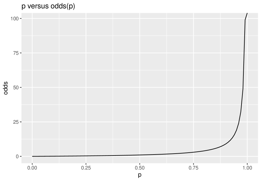
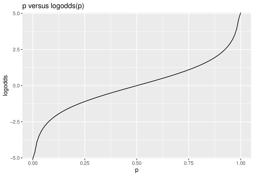
This transformation allows modeling a family of relationships between continuous predictors and a binary outcome variable, in this case, bankruptcy.

Key steps are

1. Assuming that predictors are linearly related to the log-odds

2. Transform the odds to convert to probability

3. Estimate the data likelihood

In this context, intercept shifts the curve left or right. Slopes make the curve sharper or flatter, with respect to predictors. The logistic starts at 0, ends at 1 and is symmetric around .5.

Figure 3: Logodds(p) vs p

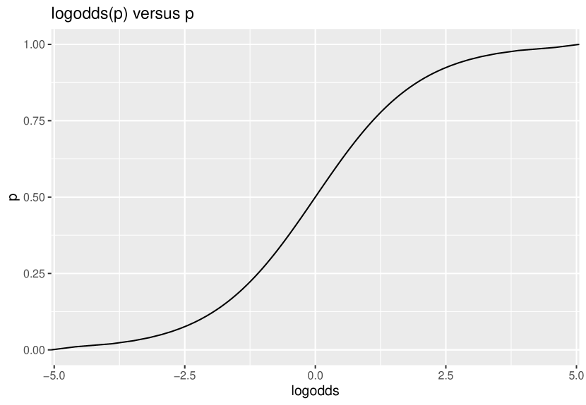
Logistic regression transforms the bankruptcy outcomes so that a linear combination of predictors produces log-odds effects on the bankruptcy. A model coefficient is transformed and interpreted as an odds multiplier. These results are easily interpretable.

The logistic regression model used in this study is based on the following mathematical definition. Bankruptcy variable coded using 1 and 0.

$$Y=\begin{cases}1&\text{bankrupt}\\ 0&\text{non-bankrupt}\end{cases}$$

Variable of interest

$$p({\bf x})=P[Y=1\mid{\bf X}={\bf x}]$$

logistic regression model.

$$\log\left(\frac{p({\bf x})}{1-p({\bf x})}\right)=\beta_{0}+\beta_{1}x_{1}+\ldots+\beta_{k-1}x_{k-1}$$

This equation is similar to linear regression with $k-1$ predictors for a total of $k$ $\beta$ parameters. Here, the left part of the equation is the log odds. This gives the probability for a bankruptcy $(Y=1)$ divided by the probability of a non-bankruptcy $(Y=0)$. When the odds are 1, both events are equally likely. Odds greater than 1 indicate bankruptcy and vice versa.

$$\frac{p({\bf x})}{1-p({\bf x})}=\frac{P[Y=1\mid{\bf X}={\bf x}]}{P[Y=0\mid{\bf X}={\bf x}]}$$

3.5 Evaluating predictive models

Researchers evaluate Bankruptcy prediction models using multiple criteria. In this thesis, we use Accuracy tables, the receiver operating characteristics (ROC) curves, and information content tests. While ROC curves inform forecasting accuracy, sensitivity, and specificity, Information content tests evaluate the bankruptcy-related information carried by the distress risk measures. The following section presents the method of each.

3.5.1 Classification accuracy tables

A perfect model classifies all observations accurately. Real models make mistakes in classification. One way to evaluate the model’s performance is its misclassification rate. Alternatively, models accuracy can be used, which measures the proportion of correction classifications

$$\text{Misclassification }(\hat{C},\text{Data})=\frac{1}{n}\sum_{i=1}^{n}I(y_{i}\neq\hat{C}({\bf x_{i}}))$$

$$I(y_{i}\neq\hat{C}({\bf x_{i}}))=\begin{cases}0&y_{i}=\hat{C}({\bf x_{i}})\\ 1&y_{i}\neq\hat{C}({\bf x_{i}})\\ \end{cases}$$

This measure is not useful in training data. This metric improves with the number of parameters and hence will be biased towards large models. This bias encourages overfitting. Hence, this metric needs to be computed on test data, unseen by the model during training.

Accuracy tables can be further split into confusion matrix, to understand the nature of misclassification. Confusion matrix categorizes the classification errors into false negatives and false positives.

Figure 4: Confusion Matrix

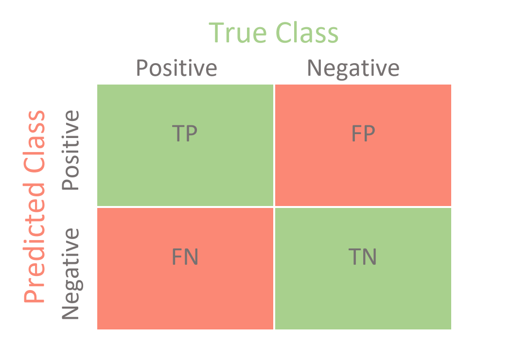
Setting the classification threshold as 0.5

$$\eta({\bf x})=0\iff p({\bf x})=0.5$$

Predictions can be used to create a confusion matrix as below.

$$\text{Prev}=\frac{\text{P}}{\text{Total Obs}}=\frac{\text{TP + FN}}{\text{Total Obs}}$$

A reasonable classifier has to outperform a naïve classifier that labels all observations as majority class. In this work, a model classifying every company as non-bankrupt will be the baseline. Apart from accuracy, specificity and sensitivity can be used to evaluate models. Sensitivity is the true-positive rate. Higher sensitivity means the model classifies more positives correctly, reducing the false negatives. Specificity is the true negative rate. Higher specificity means the classifier is labeling true negatives correctly, reducing false positives. The formulae are given below.

$$\text{Sensitivity}=\text{True Positive Rate}=\frac{\text{TP}}{\text{P}}=\frac{\text{TP}}{\text{TP + FN}}$$

$$\text{Specificity}=\text{True Negative Rate}=\frac{\text{TN}}{\text{N}}=\frac{\text{TN}}{\text{TN + FP}}$$

Both metrics can be computed directly from the confusion matrix.

Relationship between Accuracy, Specificity, and Sensitivity

As we compute specificity and sensitivity from the confusion matrix, different classification thresholds generate multiple sensitivity/ specificity values. It is normal to use 0.5 probability as “cutoff.” By modifying the cutoff, we can improve the sensitivity or specificity at the overall accuracy expense. Also, if sensitivity improves, specificity deteriorates, and vice versa.

$$\hat{C}(\bf x)=\begin{cases}1&\hat{p}({\bf x})>c\\ 0&\hat{p}({\bf x})\leq c\end{cases}$$

3.5.2 Test of predictive ability: Receiver Operating Characteristics (ROC)

Receiver Operating Characteristics (ROC) curve is a method to assess the accuracy of a continuous measurement for predicting a binary outcome. It is used extensively in the Lifesciences Domain. Over the past two decades, it gained acceptance as a bankruptcy prediction model validation tool (Sobehart and Keenan (2001)).

For a bankruptcy prediction model, for a fixed cutoff c, we can compute accuracy metrics and two types of classification errors: false negatives and false positives. In bankruptcy prediction, the model generates the measure of firm distress M, based on independent variables. This measure is a continuous measurement. We derive a 1 (test positive) classification as M exceeding a fixed threshold c: M>c. For bankruptcy detection, the binary outcome B, a good outcome of the test, is when classification is 1 (the test is positive) among bankrupt companies B=1. A bad outcome is when the classification is 1 (test is positive) among non-bankrupt companies B=0. The true-positive fraction is the probability of an estimated positive among the bankrupt firms: TPF(c)=P{M>c|B=1}. This value is the sensitivity at cutoff c. Similarly, the false-positive fraction is the probability of a bankrupt classification among the non-bankrupt firms: FPF(c)= P{M>c|B=0} ROC curve is the plot of TPF against at various cutoff levels c. It has FPF(c) on the x-axis and TPF(c) along the y-axis.

A perfect bankruptcy prediction model - that is, the ranking on default probability at cutoff c is equal to the ranking of failures at c – would be able to capture all bankruptcies. This model corresponds to a vertical line at 0 FPF. A random bankruptcy prediction model – that is, the ranking at cutoff c is not correlated with the ranking of failures – would have the same percentage of failures across each cutoff level. This model corresponds to a line at 45⁰ to the x-axis. Since we expect a bankruptcy prediction model to be better than a random model, the ROC curve is expected to be between the perfect and the random model.

To compare the two models’ predictive ability, we calculate the area under the ROC curve (AUC). Sobehart and Keenan (2001) used the AUC is the decisive indicator for default model accuracy.

3.5.3 Information Content Test

Information content tests help examine the proposed bankruptcy prediction models. They evaluate if bankruptcy prediction models carry more information than another set of variables. The use of Information content tests has many precedents in bankruptcy prediction. They complement the ROC curve analysis since (i) ROC curve analysis provides users with a binary option, but users may not be making such decisions. Users of bankruptcy prediction models are interested in determining credit terms or portfolio weights. (ii) ROC curve analysis ignores associated error costs based on context-specific type I/ type II errors.

There are two primary information criteria: the Akaike information criterion (AIC) and the Bayes information criterion (BIC). When models are built using the same data by maximum likelihood, smaller AIC or BIC indicates a better fit.

Akaike Information Criterion

The AIC is the simpler of the two; it is defined as AIC = -2LL + 2k, in which -2LL is the deviance (described below), and k is the number of predictors in the model.

The maximum log-likelihood of a regression model is: $[\log L(\boldsymbol{\hat{\beta}},\hat{\sigma}^{2})=-\frac{n}{2}\log(2\pi)-\frac{n}{2}\log\left(\frac{\text{RSS}}{n}\right)-\frac{n}{2},]$

Where $\boldsymbol{\hat{\beta}}$ and $\hat{\sigma}^{2}$ and $\text{RSS}=\sum_{i=1}^{n}(y_{i}-\hat{y}_{i})^{2}$ were selected to maximize the likelihood.

From the above, AIC is derived as the difference between penalty and log-likelihood

$[\text{AIC}=-2\log L(\boldsymbol{\hat{\beta}},\hat{\sigma}^{2})+2k=2k+n+n\log(2\pi)+n\log\left(\frac{\text{RSS}}{n}\right),]$

AIC combines two components of the model, i.e., the likelihood – a measure of “goodness-of-fit” and the penalty- proportional to the model size. The likelihood portion of AIC for two models fit on the same dataset is a function of RSS. Higher RSS (squared deviation) indicates a poor model fit. A good model has low RSS and AIC. The penalty component of AIC is $[2k,]$, a function of the number of $\beta$ parameters used in the model. As k increases, AIC increases. A good model with a small AIC will have a balance between the goodness of fit and uses a small number of parameters.

Bayesian Information Criterion

The BIC is similar to AIC but adjusts the penalty included by the number of cases: BIC = -2LL + k x log(n) in which n is the number of cases in the model. This way, BIC picks smaller models for larger sample sizes, compared to AIC. For model selection, we use the model with the smallest BIC.

$[\text{BIC}=\log(n)k-2\log L(\boldsymbol{\hat{\beta}},\hat{\sigma}^{2})=\log(n)k.+n+n\log(2\pi)+n\ log\left(\frac{\text{RSS}}{n}\right)]$

The penalty for AIC is 2k whereas for BIC, it is $[\log(n)p.]$. For datasets with $log(n)>2$ , BIC penalty will be higher compared to AIC. Hence BIC will prefer smaller models for similar log-likelihoods.

4 Results

This research work focuses on building bankruptcy prediction models using financial disclosures text features. Statistical analysis has been conducted, and models are built as per the methodology described in section 3. This chapter will describe the results.

The chapter is structured into multiple sub-sections covering descriptive statistics of linguistic features, relationship with bankruptcy, model performance, and evaluation.

4.1 Descriptive statistics

This section describes the statistical properties of datasets and features used in this work

4.1.1 Bankrupt companies

The list of bankruptcies from LoPucki (2006) has more than 1000 observations. This dataset covers large bankruptcies from 1980 to date.

The annual bankruptcy filings trend is given in figure 5.

–>

Figure 5: Number of bankruptcies filed by year

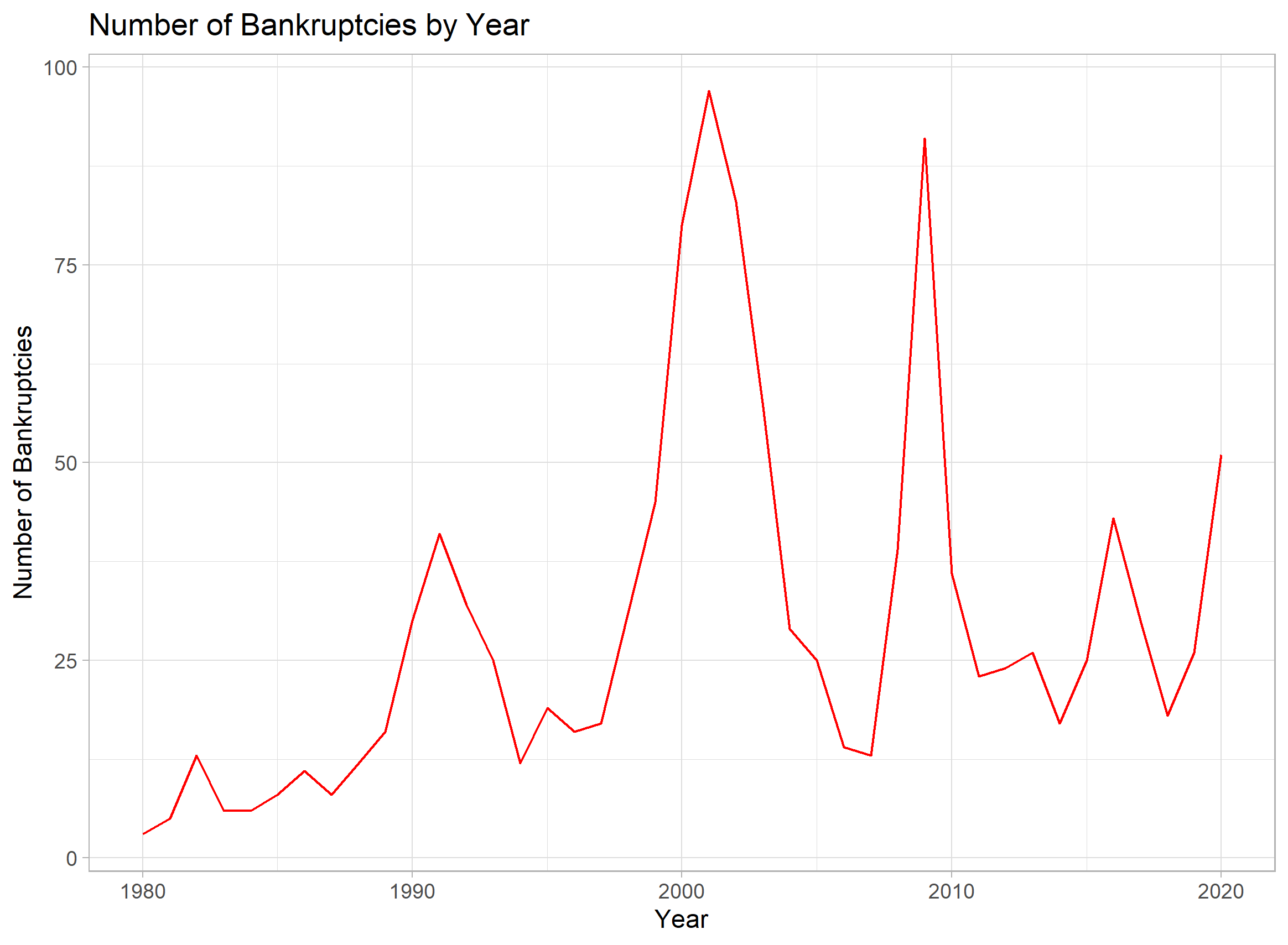
On average, 29 firms filed for bankruptcy in a year, with median annual bankruptcies at 25. A maximum of 97 bankruptcies was filed in the year 2001. Recall that this research has included bankruptcies till 2018 Dec.

4.1.2 MDA linguistic features

For the selected bankrupt firms and healthy firms, all available MDAs are transformed into numeric forms using three dictionaries, i.e., LIWC, L.M., and stress dictionary. These linguistic features are averaged at the group level and presented in the below table.

Table 2: Linguistic features words percentage

Feature	All	Bankrupt	Healthy
WPS	26.91	27.35	26.72
WC	10109.29	10164.10	10085.28
Sixltr	27.93	27.87	27.96
Dic	162.26	160.67	162.96
function.	30.57	30.67	30.52
affect	2.83	2.83	2.84
social	3.37	3.29	3.41
cogproc	7.38	7.19	7.47
percept	0.30	0.32	0.29
bio	0.98	0.97	0.98
drives	6.62	6.41	6.70
relativ	10.71	10.70	10.72
AllPunc	12.35	12.77	12.17
focuspast	1.73	1.78	1.70
focuspresent	2.69	2.61	2.73
focusfuture	0.78	0.80	0.78
anger	0.04	0.03	0.04
posemo	2.10	2.12	2.09
negemo	0.73	0.71	0.74
debt	2.72	3.04	2.58
distress	0.24	0.33	0.21
restructure	0.08	0.09	0.07
healthy	0.54	0.55	0.54
negative	1.01	1.07	0.98
positive	0.51	0.48	0.52
uncertainty	0.96	0.91	0.98

Column “All” documents the summary statistics for all sample firms. WPS and W.C. indicate that the sample firms’ MDAs are in general lengthy with ~10000 words and 27 words per sentence, indicating ~400 sentences per MDA. Excluding WPS and W.C., all other values are in percentages. Close to 30% of words are complex (27.93 Sixltr ) and functional (function. 30.57). The sample firms’ MDAs are present-focused (focuspresent 2.69), and their future focus is one-third of the present focus. Per LIWC classification, on average, the MDAs have three times more positive words compared to negative words (posemo:2.1, negemo: 0.73). Cognitive process-related and drives related words are observed with similar frequency (cogproc:7.38, drives:6.62), while Social/ affect words occur at half of that (social:3.37, affect:2.83). Based on the L.M. dictionary, we can observe that negative and uncertain words are double that of positive words frequency (negative:1.01, uncertain:0.96, positive: 0.51) Stress dictionary features indicate that debt words are prevalent at 2.72. In a typical MDA of 10,000 words length, this indicates 270 words describing debt-related discussion and disclosures. Distress and restructure related occur less frequently, which can be expected as they are infrequent organizational outcomes.

The table’s focus is Column “Bankrupt,” as it illustrates the summary statistics of bankrupt firms. Bankrupt firms are more past focused. They also use less cognitive and drives related words. A striking difference is observed in the increase in debt and distress related word frequency. They also show increased negative word frequency.

Since we are interested in building predictive models using prior year filings, it would be critical to observe how the linguistic features trend for bankrupt companies compared to non-bankrupt companies. The figure 6 shows the same.

Figure 6: Linguistic features evolution

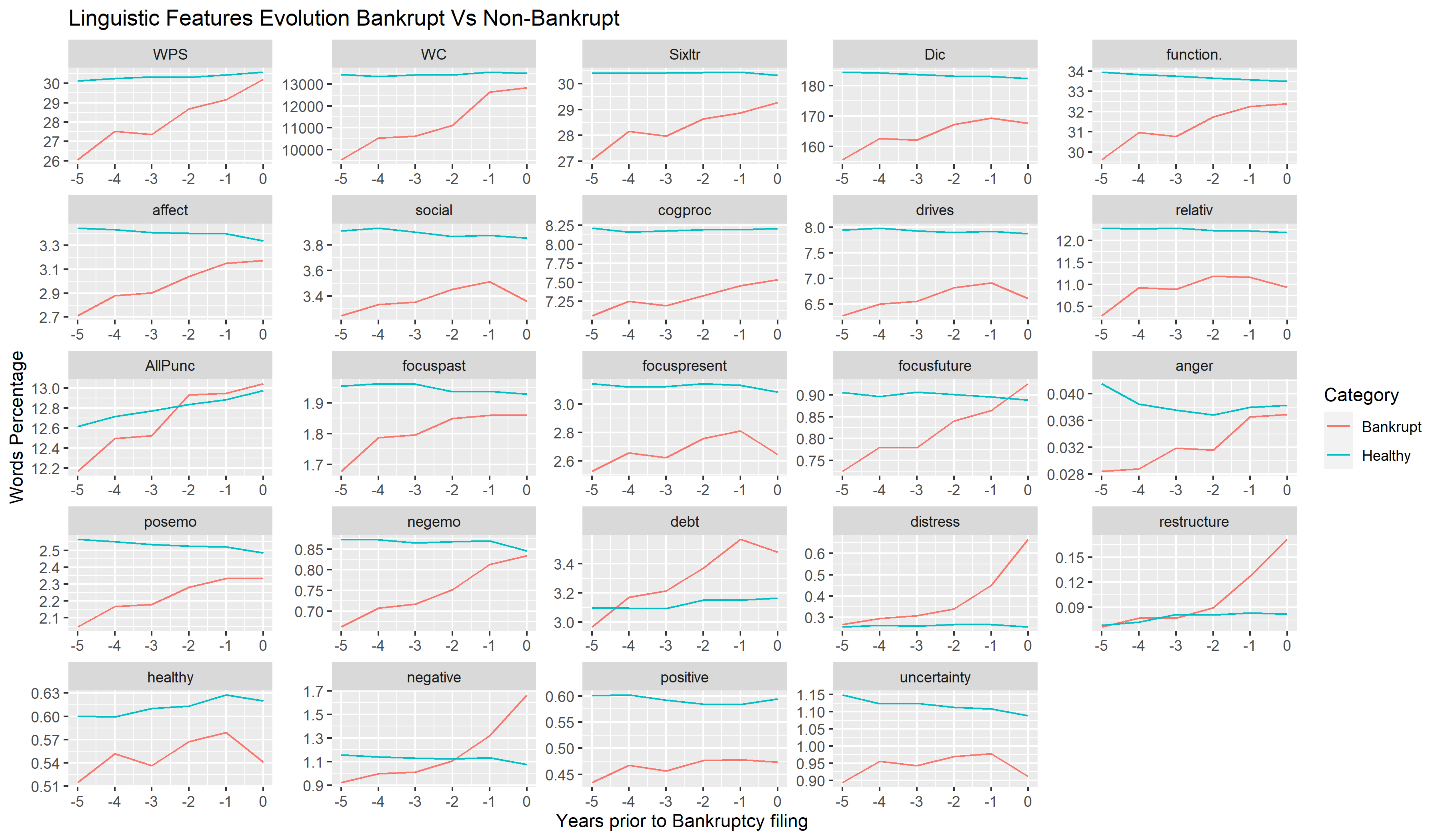
This figure depicts various types of word frequencies for bankrupt companies during the year of bankruptcy and five prior years. For comparison, sample non-bankrupt firms’ word percentages are plotted over six years, going back from the latest filing. The values are averaged for bankrupt and non-bankrupt firms.

Notable trends in LIWC features
All linguistic LIWC features for bankrupt firms are lower than non-bankrupt firms throughout the period. There is a gradual increase in focuspast and focusfuture.

Notable trends in L.M. features
Bankrupt companies have lower uncertain and positive words throughout the period. Negative words stat increasing two years before the bankruptcy.

Notable trends in Stress Dictionary features

Stress dictionary features captured the evolution of distress and bankruptcy. Debt related words exceed relative to healthy firms four years before bankruptcy and gradually inch up further till the event of bankruptcy. Distress related words remain marginally higher from 5 years to 2 years before bankruptcy and dramatically increase after that. Restructure related word frequency for bankrupt firms is indistinguishable till two years before the bankruptcy. This observation is expected as firms do not take up such costly exercises unless the financial distress is unmanageable and covenant default is imminent. There is no change in “healthy” frequency for both bankrupt and non-bankrupt firms, though bankrupt firms have lower occurrence throughout the period.

Overall, we can observe sufficient differences between bankrupt and non-bankrupt firms.

4.1.3 Correlation between linguistic features

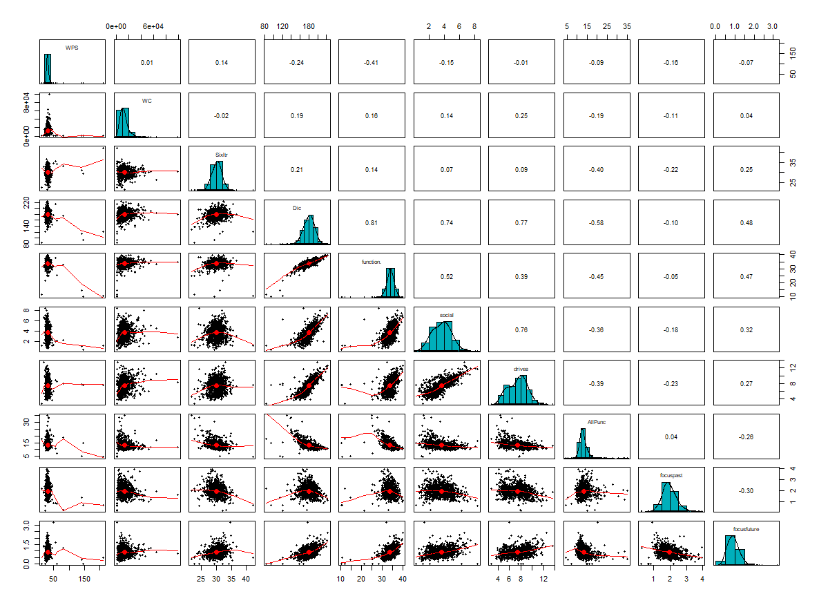
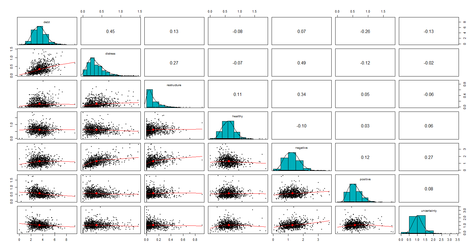
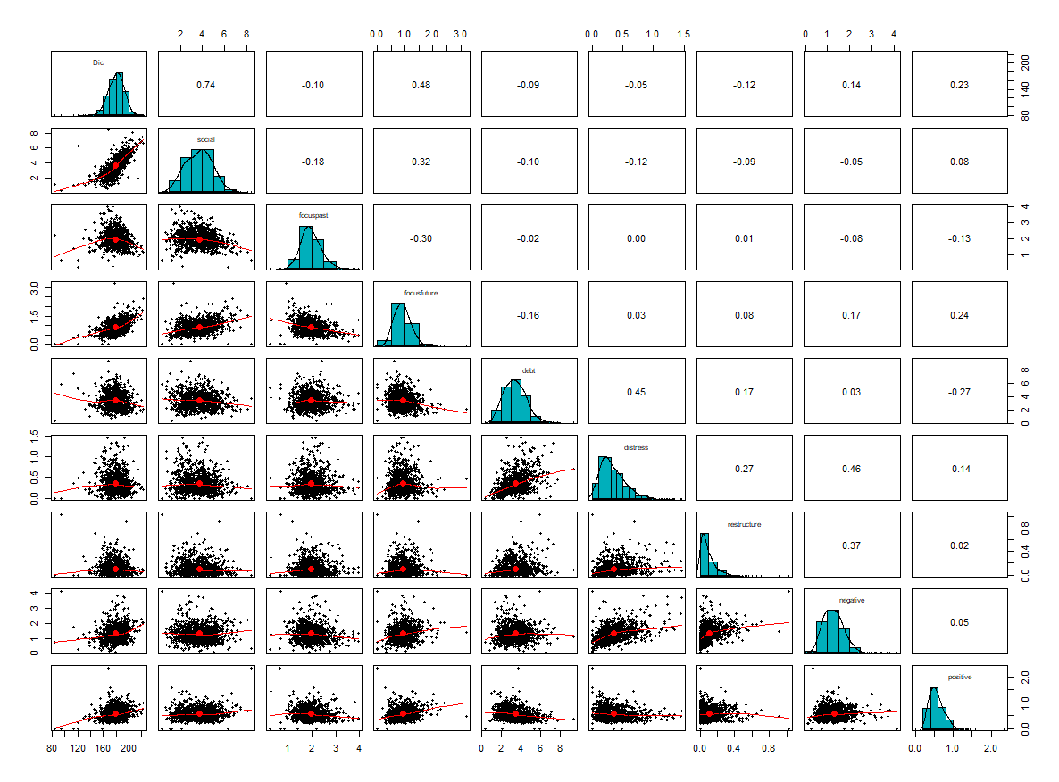
Figures 7, 8,9 show correlation structure among LIWC features, LM-Stress dictionary and selected variables from these three models.

Of the LIWC features, few are highly correlated, i.e., dictionary, functional, social, and drives. All other features have low correlations indicating they are capturing different information. In the stress dictionary, debt and distress show a 0.45 correlation, which is expected. Other variables are uncorrelated. Also, there is no correlation between the L.M. dictionary and stress dictionary features. Finally, selected variables from these three models are checked for correlation. There is an insignificant correlation indicating minimum overlap. This low correlation indicates their complementary nature, and a hybrid model combining these features might perform better than standalone models.

Figure 7: Correlations between LIWC features

Figure 8: Correlations between LM and stress dictionary

Figure 9: Correlations between all selected linguistic features

4.2 Experiment results

The following will explain the results of various experiments done to test the hypothesis we outlined in the methodology

4.3 Hypothesis 1: Linguistic differences exist between bankrupt and non-bankrupt firm’s financial disclosures

From descriptive statistics, we observed that there are distinct qualities that differentiate bankrupt firms from non-bankrupt firms. We set out to test this hypothesis.

4.3.1 Association between linguistic markers and distress

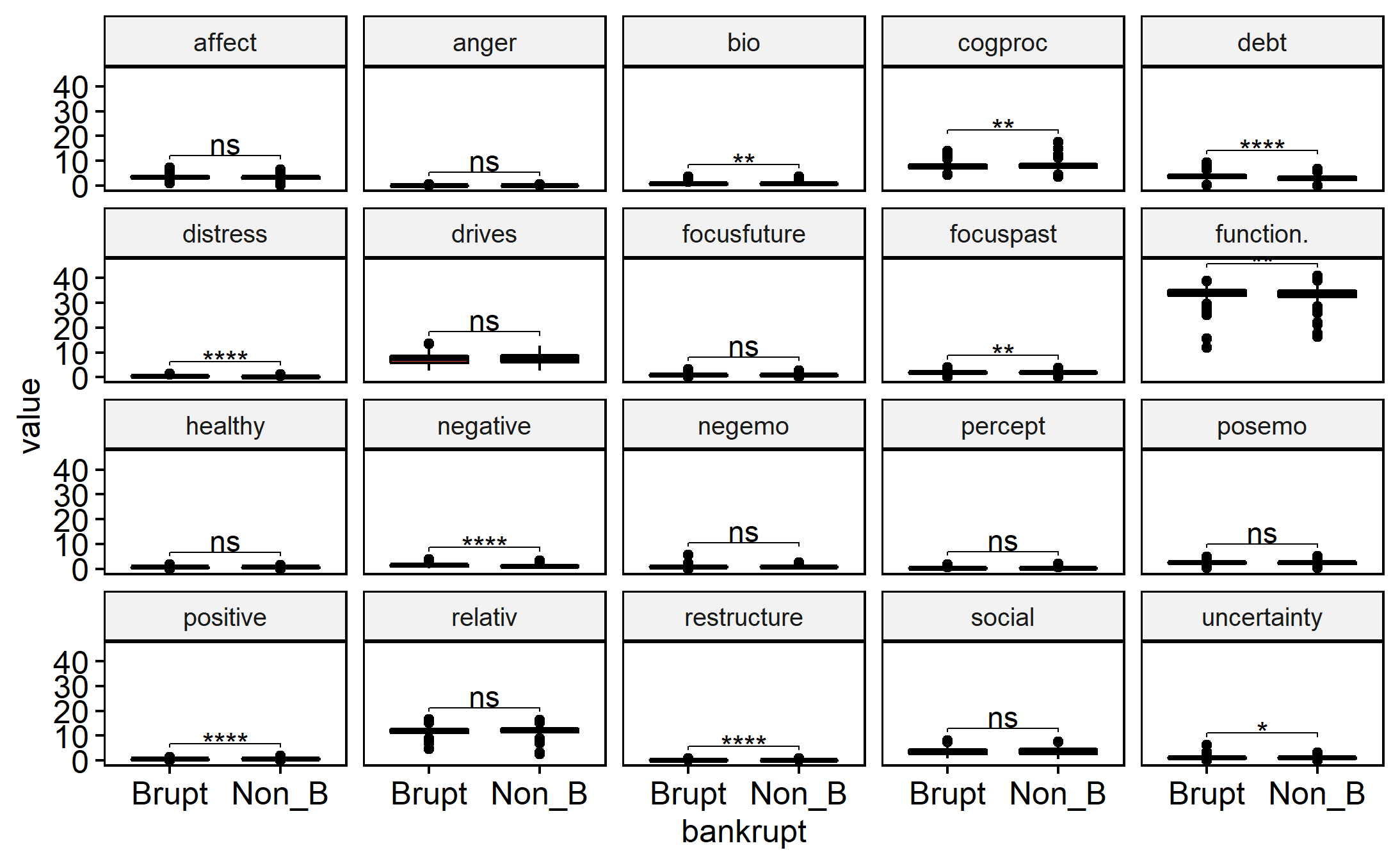
Independent T-tests were conducted. The number of bankrupt firms and non-bankrupt firms is 500 each

The 500 bankrupt firms compared to the 500 non-bankrupt firms demonstrated significantly higher distress, t(868) = 17.38, p = .00.

Bankrupt firms had significantly higher debt (t(992) = 12.32, p= 0.00), higher negative words (t(997) = 8.28, p= 0.00) and higher restructure words (t(922) = 7.67, p= 0.000)

There was no significant effect for negative emotions (negemo), t(988) = 0.69, p = .62, despite bankrupt (M = 0.88, SD = 0.38) attaining higher scores than non-bankrupt (M = 0.86, SD = 0.35).

10 shows the details.

Figure 10: Bankrupt vs non-bankrupt linguistic features T test

4.4 Hypothesis 2: Domain-specific dictionaries capture linguistic differences better than general language models

As part of this hypothesis, a Logistic regression model with all LIWC features as independent variables has been fit. Another model with L.M. features as predictors are built and compared.

4.4.1 LIWC

Here we review the LIWC logit model. Table 3 presents the model details.

We can observe that only a few predictors are significant. This observation is expected as the LIWC model captures various aspects of language, and only a few of them can be expected to be impacted by the distress and potential bankruptcy conditions. $WPS$, $Dic$, $function.$, $focuspast$, and $focusfuture$ are significant at 0.001 level. The logistic regression coefficients give the change in the log odds of the outcome for a one-unit increase in the predictor variable. Here, except $WPS$, all predictors are percentages of category words.

For every one unit change in $WPS$, the log odds of bankruptcy (versus non-bankruptcy) increases by 0.08 with 95% CI [0.04, 0.12]. For a one percent increase in $focuspast$ the log odds of being bankrupt increases by 1.10 with 95% CI [0.66, 1.55]. The same for $focusfuture$ increases by 1.65 with 95% CI [1.00, 2.31].

Another way to interpret these coefficients is to use the odds ratio. This fitted model says that holding other predictors at a fixed value, the odds of bankruptcy for a firm whose disclosure has 1% $focusfuture$ words than a firm with zero percent such words are exp(1.65) = 5.2. We can say that the odds for a firm with $1$ higher $focusfuture$ words are 420% higher in terms of percent change.

Other predictors that are significant at <0.05 levels are $social$, $cogproc$, and $drives$. The log odds are 0.37, -0.34, 0.30 with 95% CIs [0.10, 0.65], [-0.64, -0.06], and [-0.00, -0.60], respectively.

Table 3: LIWC model coefficients

Predictors	Coefficients	SE	pvalue	Lower CI	Upper CI	Odds Ratio
Intercept	2.75	3.34	0.411	-3.92	9.16	15.68
WPS	0.08	0.02	<0.001	0.04	0.12	1.08
WC	0.00	0.00	0.103	0.00	0.00	1.00
Sixltr	-0.07	0.05	0.202	-0.17	0.04	0.93
Dic	-0.16	0.04	<0.001	-0.24	-0.08	0.85
function.	0.60	0.11	<0.001	0.39	0.81	1.82
affect	-0.60	5.21	0.909	-11.50	9.26	0.55
social	0.37	0.14	0.007	0.10	0.65	1.45
cogproc	-0.34	0.15	0.021	-0.64	-0.06	0.71
percept	0.73	0.40	0.070	-0.05	1.52	2.07
bio	-0.05	0.23	0.829	-0.49	0.39	0.95
drives	0.30	0.15	0.049	0.00	0.60	1.35
relativ	-0.06	0.12	0.604	-0.29	0.17	0.94
AllPunc	-0.08	0.04	0.062	-0.16	0.00	0.92
focuspast	1.10	0.23	<0.001	0.66	1.55	3.00
focuspresent	0.06	0.21	0.773	-0.35	0.48	1.06
focusfuture	1.65	0.33	<0.001	1.00	2.31	5.20
anger	0.68	2.18	0.754	-3.57	5.05	1.98
posemo	1.15	5.21	0.825	-8.70	12.05	3.17
negemo	1.34	5.24	0.799	-8.57	12.30	3.81

Figure 11: LIWC model ROC

4.4.2 LM

Here we review the L.M. logit model. Table 4 presents the coefficients and confidence intervals.

We can observe that all predictors are significant. $negative$ and $positive$ are significant at 0.001 level. For a one percent increase in $negative$ words, the log odds of being bankrupt increases by 1.141 with 95% CI [1.08, 1.76]. The same for $positive$ changes by -2.88 with 95% CI [-3.68, -2.12].

This L.M. model says that holding other predictors at a fixed value, the odds of bankruptcy for firms whose disclosure has 1% $negative$ words than a firm with zero percent such words are exp(1.41) = 4.10. We can say that the odds for a firm with $1$ higher $negative$ words are 310% higher in terms of percent change.

Table 4: LM model coefficients

Predictors	Coefficients	SE	pvalue	Lower CI	Upper CI	Odds Ratio
Intercept	0.56	0.31	0.070	-0.04	1.17	1.75
negative	1.41	0.17	<0.001	1.08	1.76	4.10
positive	-2.88	0.40	<0.001	-3.68	-2.12	0.06
uncertainty	-0.64	0.20	0.002	-1.06	-0.26	0.53

Figure 12: LM model ROC

4.4.3 LIWC and L.M. model comparison

ANOVA indicates that models are significantly different.

Accuracy, BIC, and AIC metrics

Table 5: LIWC and LM model comparison

Model	Training Accuracy	Test Accuracy	LogLik	AIC	BIC	AUC	Deviance	Parameters
LIWC	0.69	0.63	-470.61	981.22	1074.92	0.72	941.22	19
LM	0.68	0.74	-489.88	987.75	1006.49	0.78	979.75	3

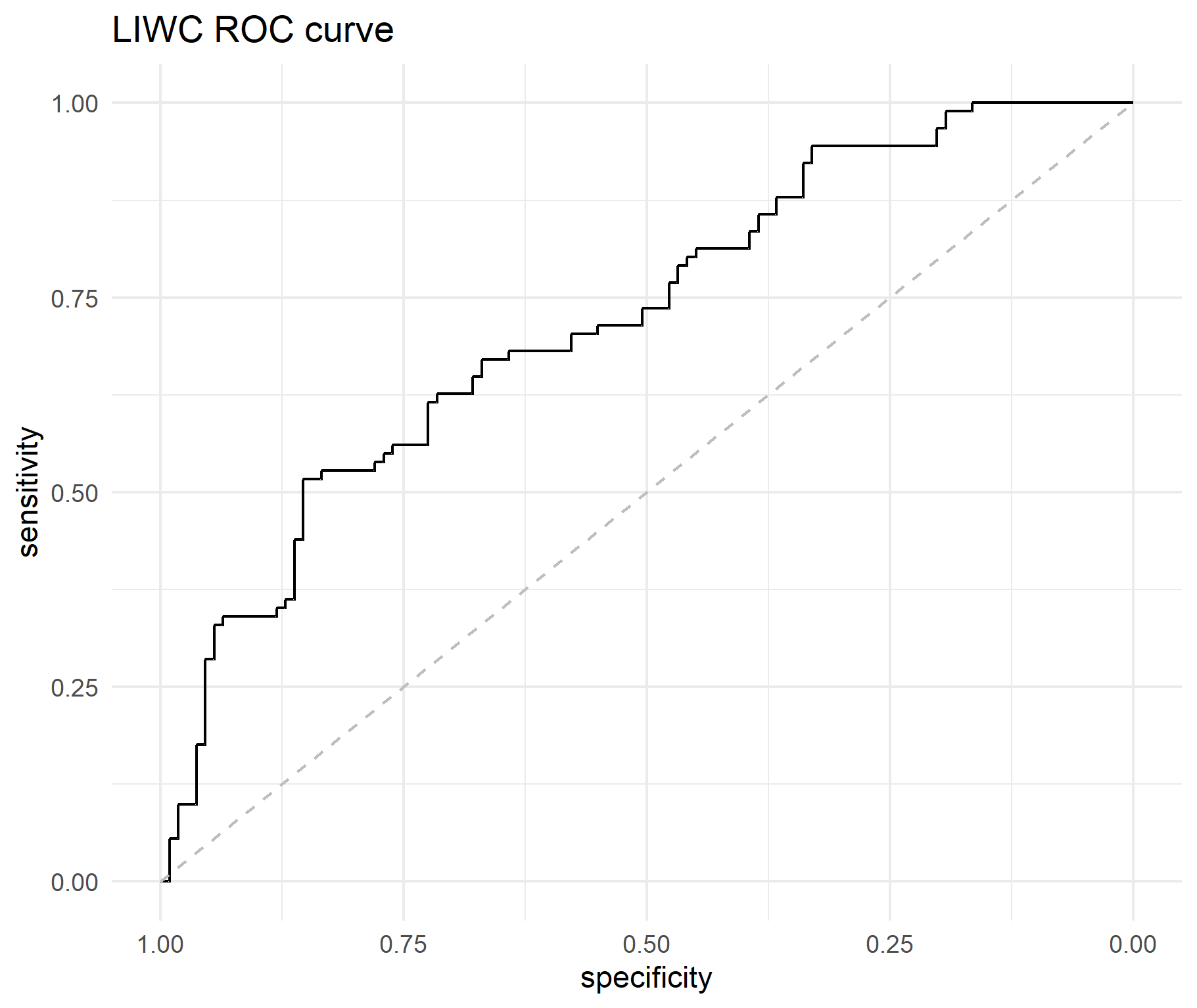
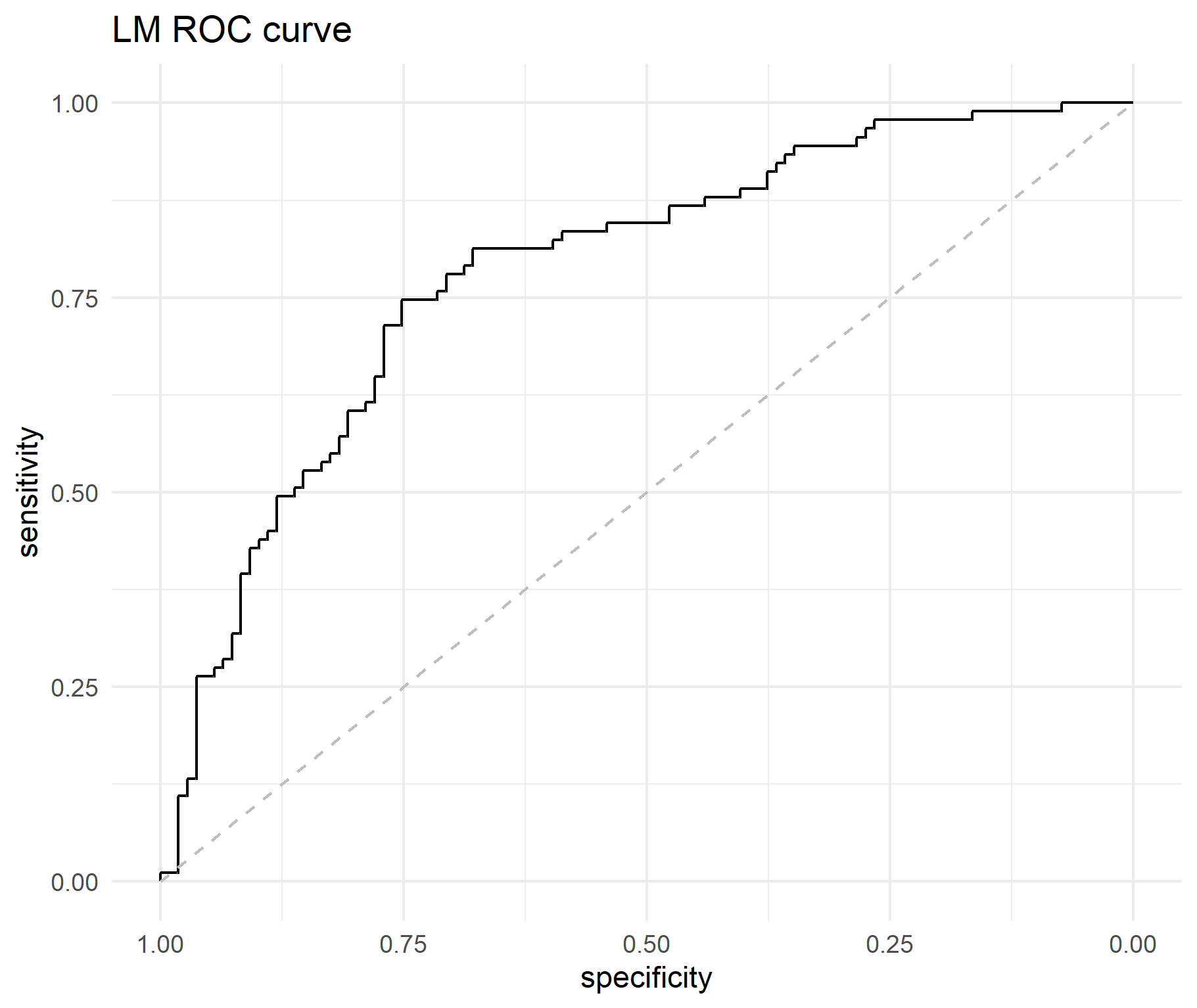
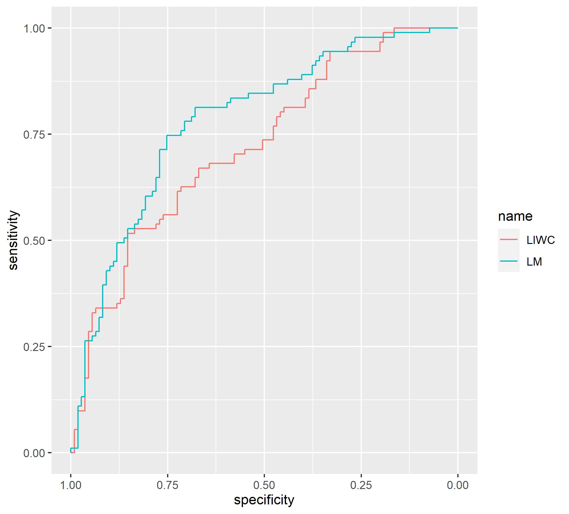
ROC comparison is shown in figure 13

We can observe that for the L.M. model, while BIC is lower than the LIWC model, AIC is higher. Recall that we noted in section 3.5.3, for sample size >100, BIC will prefer smaller models for similar log-likelihoods. The out of sample forecasting performance represented in the Test Accuracy column indicates the L.M. model provides 10% higher accuracy. Also, ROC is better for L.M. Overall, while the LIWC model captures more information, probably due to many parameters, the L.M. model predictive performance is better than the LIWC model.

Figure 13: LIWC LM ROC comparison

4.5 Hypothesis 3: Task-specific dictionaries capture linguistic differences better than domain-specific dictionaries

4.5.1 Stress dictionary

Here we review the stress dictionary logit model. Table 6 presents the coefficients and confidence intervals.

We observe that $debt$, $distress$ and $restructure$ are significant at 0.001 level. For a one percent increase in $distress$ words, the log odds of being bankrupt increases by 5.03 with 95% CI [3.98, 6.15]. The same for $debt$, $restructure$ increase by 0.36 and 2.96 with 95% CIs [0.19, 0.54] and [1.45, 4.54] respectively.

Most importantly, as per this model, holding other predictors at a fixed value, the odds of bankruptcy for a firm whose disclosure has 1% $distress$ words compared to a firm with zero percent such words is exp(5.03) = 153.66. This high odds ratio indicates that distress words percentage is a highly sensitive indicator to forthcoming bankruptcy.

Table 6: Stress dictionary model coefficients

Predictors	Coefficients	SE	pvalue	Lower CI	Upper CI	Odds Ratio
Intercept	-3.36	0.40	<0.001	-4.16	-2.59	0.03
debt	0.36	0.09	<0.001	0.19	0.54	1.44
distress	5.03	0.55	<0.001	3.98	6.15	153.66
restructure	2.96	0.79	<0.001	1.45	4.54	19.39
healthy	0.23	0.38	0.5	-0.51	0.98	1.26

Figure 14: Stress dictionary model ROC

4.5.2 Stress dictionary vs. L.M.

Table 7: Stress and LM model comparison

Model	Training Accuracy	Test Accuracy	LogLik	AIC	BIC	AUC	Deviance	Parameters
LM	0.68	0.74	-489.88	987.75	1006.49	0.78	979.75	3
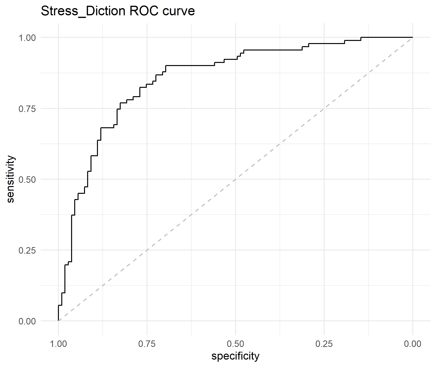
Stress_Diction	0.72	0.79	-428.09	866.18	889.61	0.86	856.18	4

ROC comparison is shown in figure 15 Overall, we can observe that the Stress model is better than the L.M. model on BIC and ROC criteria. Also, test performance is better in the Stress dictionary.

Figure 15: LM and stress dictionary model ROC comparison

4.5.3 Hypothesis 3.1: Combination models outperform individual dictionary models

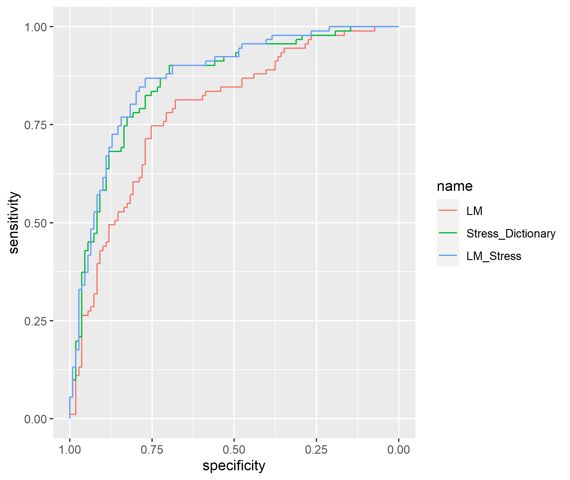
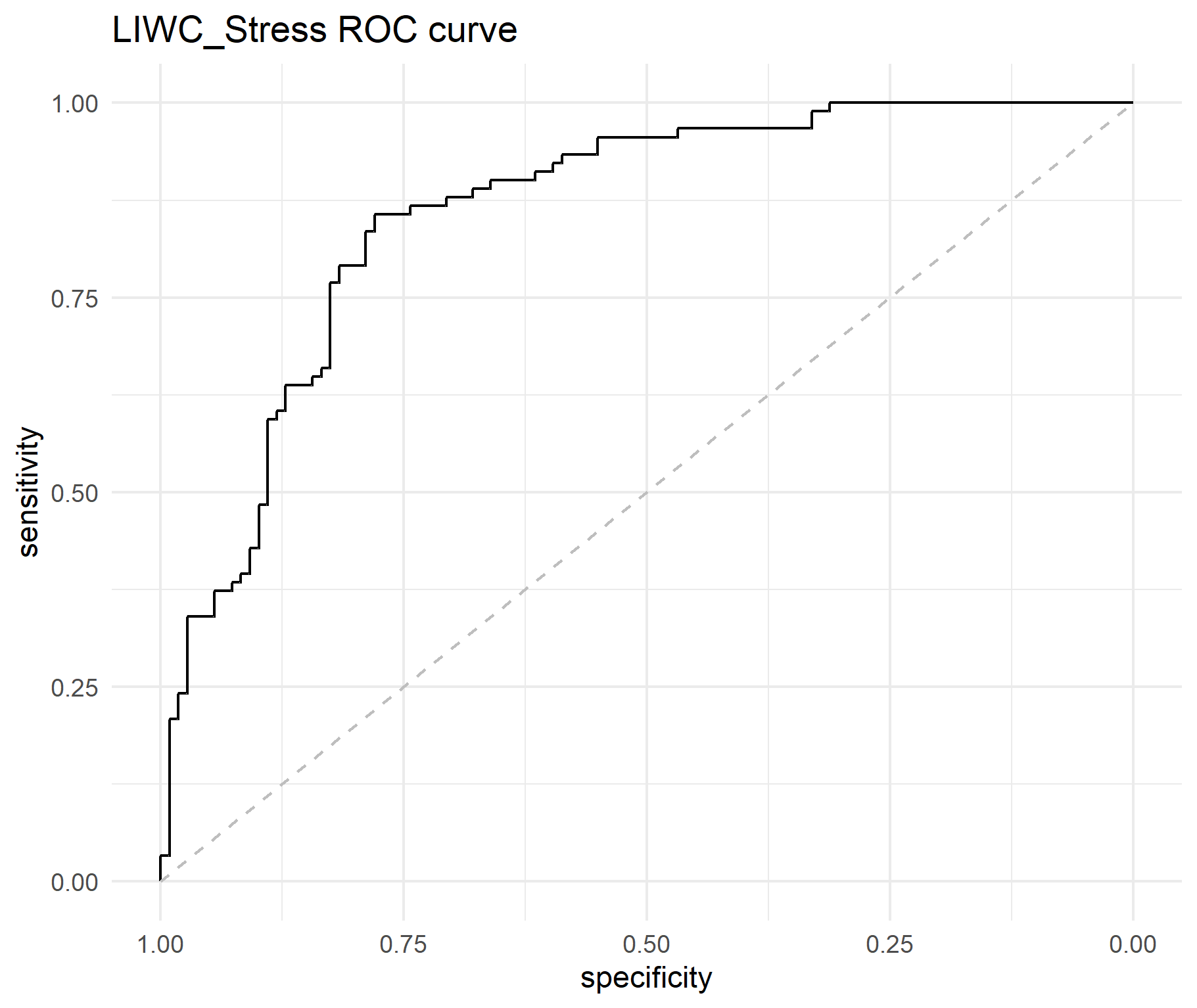
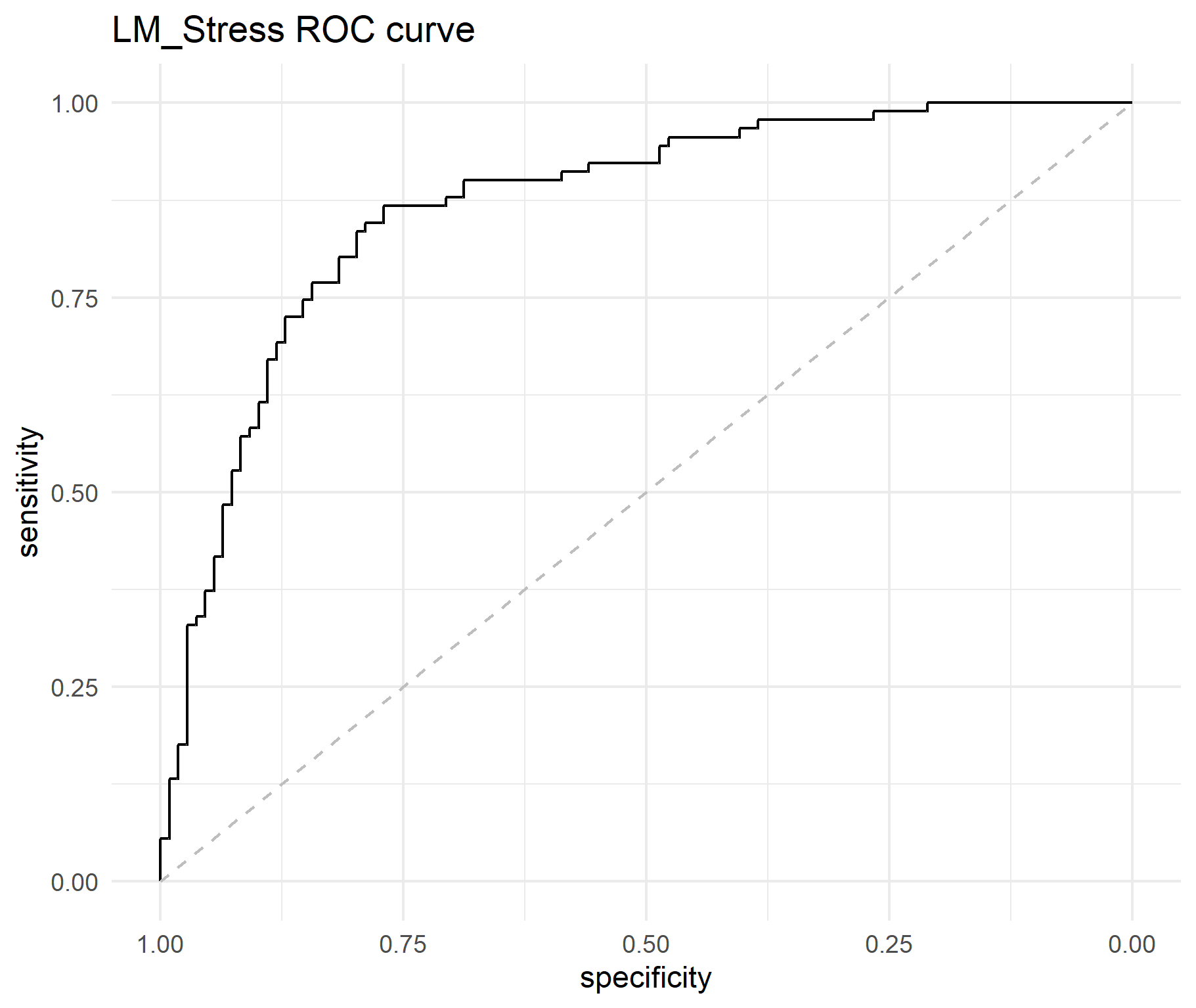
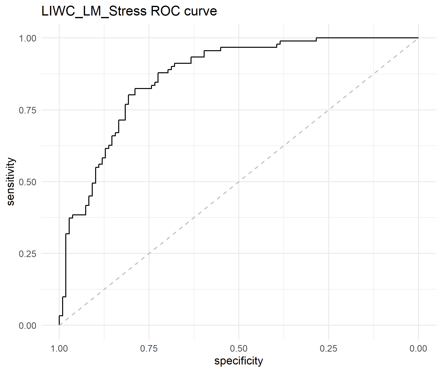
Considering the observation that the Correlation between LIWC, L.M., and stress dictionary features is low, we can take advantage of their complementary nature. Three combination models with combined inputs have been fitted on the dataset: LIWC + Stress, L.M. + Stress, and LIWC + L.M. + Stress. Model coefficients are presented in appendix B. The performance results are shared below.

Combination models

Table 8: Dictionary models AUC comparison

Model	AUC
LIWC	0.72
LM	0.78
Stress_Diction	0.86
LIWC_Stress	0.86
LM_Stress	0.87
LIWC_LM_Stress	0.87

Figure 16: LIWC and stress dictionary model ROC

Figure 17: LM and stress dictionary model ROC

Figure 18: LIWC, LM and stress dictionary model ROC comparison

4.5.4 Summary of dictionary-based models

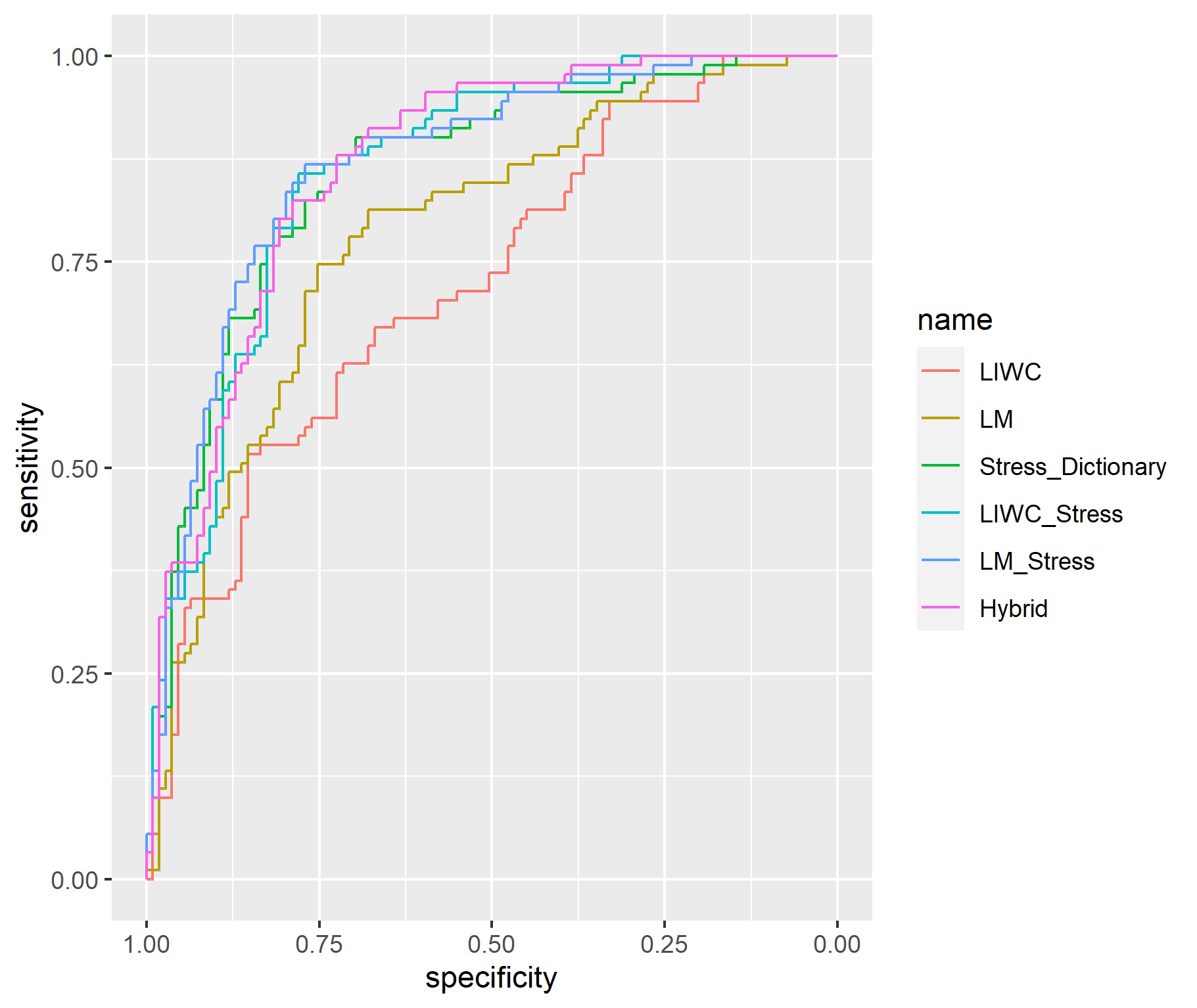
This subsection reviews the dictionary-based models. We have evidence to believe that there is incremental performance improvement as additional features are incorporated into the model. A comparison of model performance is as below

Table 9: Dictionary models comparison

Model	Training Accuracy	Test Accuracy	LogLik	AIC	BIC	AUC	Deviance	Parameters
LIWC_LM_Stress	0.78	0.80	-366.95	787.89	914.38	0.87	733.89	26
LIWC_Stress	0.77	0.79	-374.89	797.78	910.21	0.86	749.78	23
LM_Stress	0.74	0.80	-410.58	837.17	874.64	0.87	821.17	7
Stress_Diction	0.72	0.79	-428.09	866.18	889.61	0.86	856.18	4
LIWC	0.69	0.63	-470.61	981.22	1074.92	0.72	941.22	19
LM	0.68	0.74	-489.88	987.75	1006.49	0.78	979.75	3

Figure 19: Bag of words dictionary models ROC comparison

5 Discussion

This work provides the first comprehensive test of text disclosure-based dictionary-based bankruptcy prediction models. For Dictionary-based models, I apply the LIWC dictionary Pennebaker et al. (2015), the Loghron McDonalds Dictionary Loughran and Mcdonald (2011), and a custom dictionary, developed as part of this work. To test the models’ performance, I use receiver operating characteristics (ROC) curves, information content tests, and the accuracy metrics.

The tests using ROC curve analysis demonstrated that all dictionary-based bankruptcy prediction models have a greater forecasting accuracy than a random model and that the composite models perform better than their individual language models. Information content tests provide evidence that all models carry significant bankruptcy-related information.

6 Conclusion

In this chapter, I summarize the contributions of the current study to text analysis in finance, present the research’s objectives and findings in the context of previous research, and suggest appropriate future research directions.

6.1 Objectives and summary of research

This study constitutes an exploration of knowledge extraction from the narrative, corporate report sections using text analysis. The aims are

1.To establish if linguistic features of disclosures can explain firm attributes in the financial analysis context
2.To determine which language models perform better in capturing information.
3.Specifically, to predict bankruptcy based on management’s discussion and analysis in annual filings.

Knowledge in a public firm’s context involves information that can influence organizational outcomes and future stock performance. As managers have an information advantage over the public, their narrative disclosures have significant information content, over and above the quantitative financial measures. This information helps in understanding the firm’s current financial status, the firm’s ability to continue its operations without hindrances, the kinds of risks the firm is exposed to, strategic and tactical interventions the management is undertaking to overcome the challenges capture the opportunities and capital allocation plans. This knowledge gives more in-depth insights into the firm’s prospects.

In the context of this thesis, knowledge extraction is studied in the form of predicting adverse organizational outcomes, specifically in the form of (1) Bankruptcy prediction, i.e., predict if a firm will file for chapter 7 or 11 within one year after the annual filing date (2) using management disclosures and analysis section in annual filing (10-K).

For this purpose, I employed one new measurement technique based on content analysis and research, namely a stress score based on the number of financial stress words per thousand words. I built text feature-based bankruptcy prediction models LIWC dictionary, L.M. dictionary, and Stress dictionary. Concerning the text feature-based bankruptcy prediction introduced in this study, this is the first time they are used in accounting research, and they address the numbers bias concerns inherent in traditional approaches. The scoring of Stress using linguistic markers is also a new approach to measuring financial distress. It is based on the linguistic characteristics that management displays when explaining the current liquidity challenges and its attempts to overcome them through debt extensions, new financing, and asset restructuring. Such explanations would result in increased frequencies of words related to covenants, modified loan agreements, restructuring, new financing activities, uncertainty about firms’ ability to raise funds, asset sales, and capital expense reduction in a distressed corporate reporting context. It may also result in management attempting to present a rosy image of prospects to outsiders inconsistent with management’s perception of the firm and its performance.

6.2 Summary of result and comparison with previous research findings

Bankruptcy prediction has been an active research topic for accounting researchers over decades. With the improved awareness about financial ratios’ shortcomings and availability of text analysis tools, researchers have explored incorporating textual features into bankruptcy prediction models. Hájek and Olej (2015) studied various word categories from corporate annual reports and showed that the language used by bankrupt companies shows stronger tenacity, accomplishment, familiarity, present concern, exclusion, and denial. They built prediction models combining both financial indicators and word categorizations as input variables.

Working on U.S. Banks Gandhi, Loughran, and McDonald (2017) used disclosure text sentiment as a proxy for bank distress. Other notable works using text analysis for bankruptcy prediction were Yang, Dolar, and Mo (2018) and Mayew, Sethuraman, and Venkatachalam (2015). Yang, Dolar, and Mo (2018) used high-frequency words from MDA and compared the differences between bankrupt and non-bankrupt companies. Mayew, Sethuraman, and Venkatachalam (2015) also analyzed MDA with a focus on going-concern options. They found that disclosure’s predictive ability is incremental to financial ratios, market-based variables, even the auditor’s going concern opinion and extends to three years before the bankruptcy.
As we can observe, prior work focused on marginal information content in the text. While researchers concluded that narratives have information content and predictive power, the limits and extent of that information are not tested. This thesis tests that and demonstrates that the information content is sufficient to predict bankruptcy, independent of any financial and quantitative metrics.

Prior work in disclosure text analysis focused on simple text measures like readability, sentiment, and tone. This limitation was probably motivated by the intent to use them as marginal predictors, along with financial ratios. Also, the language model methods were the limitation. Limited organizational outcomes can be explained by shallow language models that capture marginal information from disclosure text. My work has demonstrated that interpretable and accurate predictions can be made with task-specific dictionaries.

6.3 Implications of research findings

This work demonstrates that textual disclosures, independent of financial ratios, have predictive power. Further, by way of task-independent language models, this work enables multiple tasks to be solved with the same set of features, i.e., language features. With a sufficiently large dataset containing 100s of samples, researchers can build reliable predictive models quickly.

Another implication is text-based soft metrics. Investors are interested in knowing firm performance on corporate responsibility, climate change, and ethical business practices. It is not easy to measure these attributes using accounting metrics. Capturing and reporting new metrics will involve significant capital expenditure for firms. Firms can report the same using narrative disclosures. Investors can extract the same using the methods shown in this work. Finally, text metrics-based factors and factor investment is a possibility based on this approach. Lopez Lira (2019) used text-based analysis to measure firm risk exposure and built factor models with such risk portfolios. These models explain cross-section returns suggesting internal validity. Similar portfolios on other dimensions like fraud, climate exposure, etc., can be explored using this thesis’s approach.

6.4 Limitations of research

Like other empirical studies in finance and language processing, the results presented in this thesis contain some limitations.

Due to resource constraints for downloading, processing, and storing extensive text data, the Knowledge extraction from Financial disclosures has been attempted on a single task of Bankruptcy Prediction using different methodologies. I also restricted the text content to one type of corporate narrative document (i.e., Management’s Discussion and Analysis). For this reason, caution needs to be applied in generalizing results.

Since the text analysis is restricted to the surface structure of language, it is impossible to say whether the extracted signal is a true reflection of the management’s statement. What is more, disclosure changes can result from managerial interventions, restructuring activities, e.g., raising capital, asset sell-off or cost reductions, and analyzing. These interventions can improve performance, and the distressed firm might show better market performance, hence avoiding bankruptcy.

I use the EDGAR filing date as the time stamp for filing. If bankruptcy filing happens within one such filing date, such filing is used to compute linguistic features, subsequently used as predictors. Any actions that management takes after filing, which can alter firm stress levels, are not captured. This limitation is inherent when using disclosure data.

6.5 Suggestions for further research

The majority of prior text analysis research in the finance context focuses solely on sentiment analysis and does not address direct knowledge extraction. In particular, significant effort has been deployed in linking sentiment and tone to subsequent performance and fraud. Moreover, the extracted information, i.e., sentiment score, is used only as an additional input to existing quantitative models. I see four broad questions that need to be addressed. Given that management has an information advantage about firms

1.What knowledge can be extracted from the management’s textual disclosures?
2.Which of the firm’s future states can disclosures textual analysis explain or predict?
3.Which language and document models facilitate fast and reliable information extraction?
4.How can investors incorporate this information into their decision-making process?

These research questions have received relatively less attention by comparison with efforts to measure sentiment. Improving the affordability of data science tools is making unstructured analysis easier. Wider adoption of unstructured analysis will allow researchers to apply more focus to these four questions.

6.5.1 Theoretical perspectives

My work demonstrates that textual disclosures, independent of financial ratios, have predictive power. This observation raises the question: of all available financial and accounting metrics, which can be replaced with more reliable text-based metrics? Text-based metrics can not possibly possess all the information contained in accounting metrics. However, it is critical to understand the limits of such information as well as validity.

Altman, Edward I. 1968. “Financial Ratios, Discriminant Analysis and the Prediction of Corporate Bankruptcy.” The Journal of Finance 23 (4): 589–609.

Altman, Edward I, and Edith Hotchkiss. 2010. Corporate Financial Distress and Bankruptcy: Predict and Avoid Bankruptcy, Analyze and Invest in Distressed Debt. Vol. 289. John Wiley & Sons.

Amel-Zadeh, Amir, and Jonathan Faasse. 2016. “The Information Content of 10-K Narratives: Comparing MD&A and Footnotes Disclosures.” https://doi.org/10.2139/ssrn.2807546.

Ball, Christopher, Gerard Hoberg, and Vojislav Maksimovic. 2012. “Redefining Financial Constraints: A Text-Based Analysis.” SSRN Electronic Journal. https://doi.org/10.2139/ssrn.1923467.

Beams, Joseph, and Yun Chia Yan. 2015. “The effect of financial crisis on auditor conservatism: US evidence.” Accounting Research Journal 28 (2): 160–71. https://doi.org/10.1108/ARJ-06-2013-0033.

Benoit, Kenneth, Kohei Watanabe, Haiyan Wang, Paul Nulty, Adam Obeng, Stefan Müller, and Akitaka Matsuo. 2018. “Quanteda: An R Package for the Quantitative Analysis of Textual Data.” Journal of Open Source Software 3 (30): 774. https://doi.org/10.21105/joss.00774.

Bodnaruk, Andriy, Tim Loughran, and Bill McDonald. 2013. “Using 10-K Text to Gauge Financial Constraints.” Ssrn 50 (4): 623–46. https://doi.org/10.2139/ssrn.2331544.

Bourveau, Thomas, Yun Lou, and Rencheng Wang. 2018. “Shareholder Litigation and Corporate Disclosure: Evidence from Derivative Lawsuits.” Journal of Accounting Research 56 (3): 797–842. https://doi.org/10.1111/1475-679X.12191.

Enev, Maria. 2017. “Going Concern Opinions and Management’s Forward Looking Disclosures: Evidence from the MD&A.” https://doi.org/10.2139/ssrn.2938703.

Feldman, Ronen, Suresh Govindaraj, Joshua Livnat, and Benjamin Segal. 2008. “The Incremental Information Content of Tone Change in Management Discussion and Analysis.” https://doi.org/10.2139/ssrn.1126962.

———. 2010. “Management’s tone change, post earnings announcement drift and accruals.” Review of Accounting Studies 15 (4): 915–53. https://doi.org/10.1007/s11142-009-9111-x.

Fisher, Ingrid E, Margaret R Garnsey, and Mark E Hughes. 2016. “Natural Language Processing in Accounting, Auditing and Finance: A Synthesis of the Literature with a Roadmap for Future Research.” Intelligent Systems in Accounting, Finance and Management 23 (3): 157–214.

Gandhi, Priyank, Tim Loughran, and Bill McDonald. 2019. “Using Annual Report Sentiment as a Proxy for Financial Distress in Us Banks.” Journal of Behavioral Finance 20 (4): 424–36.

———. 2017. “Using Annual Report Sentiment as a Proxy for Financial Distress in U.S. Banks.” Ssrn, March, 1–13. https://doi.org/10.2139/ssrn.2905225.

Hájek, Petr, and Vladimír Olej. 2015. “Word categorization of corporate annual reports for bankruptcy prediction by machine learning methods.” In Lecture Notes in Computer Science (Including Subseries Lecture Notes in Artificial Intelligence and Lecture Notes in Bioinformatics), 9302:122–30. https://doi.org/10.1007/978-3-319-24033-6_14.

Hillegeist, Stephen A, Elizabeth K Keating, Donald P Cram, and Kyle G Lundstedt. 2004. “Assessing the Probability of Bankruptcy.” Review of Accounting Studies 9 (1): 5–34.

Huizinga, Harry, and Luc Laeven. 2012. “Bank Valuation and Accounting Discretion During a Financial Crisis.” Journal of Financial Economics 106 (3): 614–34.

Lopatta, Kerstin, Mario Albert Gloger, and Reemda Jaeschke. 2017. “Can Language Predict Bankruptcy? The Explanatory Power of Tone in 10-K Filings.” Accounting Perspectives 16 (4): 315–43. https://doi.org/10.1111/1911-3838.12150.

Lopez Lira, Alejandro. 2019. “Risk Factors That Matter: Textual Analysis of Risk Disclosures for the Cross-Section of Returns.” https://doi.org/10.2139/ssrn.3313663.

LoPucki, Lynn M. 2006. “Bankruptcy Research Database.”

Loughran, Tim, and Bill Mcdonald. 2009. “Plain English , Readability , and 10-K Filings.” English.

Loughran, T I M, and Bill Mcdonald. 2011. “When is a Liability not a Liability ? Textual Analysis , Dictionaries , and 10-Ks Journal of Finance , forthcoming.” 1. Vol. 66. https://doi.org/10.1111/j.1540-6261.2010.01625.x.

Mayew, William J., Mani Sethuraman, and Mohan Venkatachalam. 2015. “MD&A disclosure and the firm’s ability to continue as a going concern.” Accounting Review 90 (4): 1621–51. https://doi.org/10.2308/accr-50983.

Nguyen, Ba-Hung, and Van-Nam Huynh. 2020. “Textual Analysis and Corporate Bankruptcy: A Financial Dictionary-Based Sentiment Approach.” Journal of the Operational Research Society, 1–20.

Pennebaker, James W, Ryan L Boyd, Kayla Jordan, and Kate Blackburn. 2015. “The Development and Psychometric Properties of Liwc2015.”

Pennebaker, James W, Martha E Francis, and Roger J Booth. 2001. “Linguistic Inquiry and Word Count: LIWC 2001.” Mahway: Lawrence Erlbaum Associates 71 (2001): 2001.

Rajan, Uday, Amit Seru, and Vikrant Vig. 2015. “The Failure of Models That Predict Failure: Distance, Incentives, and Defaults.” Journal of Financial Economics 115 (2): 237–60.

Shirata, Cindy Yoshiko, Hironori Takeuchi, Shiho Ogino, and Hideo Watanabe. 2011. “Extracting Key Phrases as Predictors of Corporate Bankruptcy: Empirical Analysis of Annual Reports by Text Mining.” Journal of Emerging Technologies in Accounting 8 (1): 31–44. https://doi.org/10.2308/jeta-10182.

Sobehart, Jorge, and Sean Keenan. 2001. “Measuring Default Accurately.” Risk 14 (3): 31–33.

Tao, Jie, Amit V. Deokar, and Ashutosh Deshmukh. 2018. “Analysing forward-looking statements in initial public offering prospectuses: a text analytics approach.” Journal of Business Analytics 1 (1): 54–70. https://doi.org/10.1080/2573234x.2018.1507604.

Tinoco, Mario Hernandez, and Nick Wilson. 2013. “Financial Distress and Bankruptcy Prediction Among Listed Companies Using Accounting, Market and Macroeconomic Variables.” International Review of Financial Analysis 30: 394–419.

Wu, Yanhui, Clive Gaunt, and Stephen Gray. 2010. “A Comparison of Alternative Bankruptcy Prediction Models.” Journal of Contemporary Accounting & Economics 6 (1): 34–45.

Yang, Fang, Burak Dolar, and Lun Mo. 2018. “Textual Analysis of Corporate Annual Disclosures: A Comparison between Bankrupt and Non-Bankrupt Companies.” Journal of Emerging Technologies in Accounting 15 (1): 45–55. https://doi.org/10.2308/jeta-52085.