Non-minimally Coupled Scalar $k$-Inflation Dynamics

Abstract

In this work we shall study $k$-inflation theories with non-minimal coupling of the scalar field to gravity, in the presence of only a higher order kinetic term of the form $\sim\mathrm{const}\times X^{\mu}$, with $X=\frac{1}{2}\partial_{\mu}\phi\partial^{\mu}\phi$. The study will be focused in the cases where a scalar potential is included or is absent, and the evolution of the scalar field will be assumed to satisfy the slow-roll or the constant-roll condition. In the case of the slow-roll models with scalar potential, we shall calculate the slow-roll indices, and the corresponding observational indices of the theory, and we demonstrate that the resulting theory is compatible with the latest Planck data. The same results are obtained in the constant-roll case, at least in the presence of a scalar potential. In the case that models without potential are considered, the results are less appealing since these are strongly model dependent, and at least for a power-law choice of the non-minimal coupling, the theory is non-viable. Finally, due to the fact that the scalar and tensor power spectra are conformal invariant quantities, we argue that the Einstein frame counterpart of the non-minimal $k$-inflation models with scalar potential, can be a viable theory, due to the conformal invariance of the observational indices. The Einstein frame theory is more involved and thus more difficult to work with it analytically, so one implication of our work is that we provide evidence for the viability of another class of $k$-inflation models.

I Introduction

The striking GW170817 event GBM:2017lvd in 2017 verified in a direct way the propagation of astrophysical gravitational waves emitted from the merging of compact astrophysical objects. Apart from generating a new scientific direction in modern astrophysics, that of gravitational wave astronomy, the GW170817 event had significant theoretical implications in the field of astrophysics and cosmology, due to the fact that it imposed serious restrictions on several modified gravity theoretical frameworks. Particularly, the most striking result from a theoretical point of view was the fact that the gravitational waves and the gamma rays emitted from the merging of the two neutron stars arrived simultaneously, so this result ruled out many theories of Horndeski type, see Ref. Ezquiaga:2017ekz for an extensive analysis along this research line.

However, there are still many modified gravity theories which still yield a gravitational wave speed $c_{T}^{2}=1$ in natural units, such as $f(R)$ gravity, $f(G)$ Gauss-Bonnet theories and so on. For an extensive account on modified gravity theories, we refer the reader to Refs. Nojiri:2017ncd ; Nojiri:2010wj ; Nojiri:2006ri ; Capozziello:2011et ; Capozziello:2010zz ; delaCruzDombriz:2012xy ; Olmo:2011uz . In addition, modified gravity theories can actually provide a theoretical framework that makes possible the description and in some cases the unification of the two acceleration eras of our Universe, such as $f(R)$ gravity for example. The modification of Einstein-Hilbert gravity seems compelling, at least when cosmological scales are considered. In fact, although Einstein-Hilbert gravity seems to describe accurately to a great extent the current perception of astrophysical scales physics, it seems that at large scales needs to be modified. Indeed, the dark energy era in the context of simple Einstein-Hilbert gravity requires the introduction of phantom scalar fields, and exotic phenomena follow, such us the existence of late-time finite time singularities. In the context of modified gravity, the inflationary era and the late-time acceleration era can be harbored under the unified framework of a single theory Nojiri:2003ft .

One class of the remaining viable gravitational theories after the GW170817 event, is the $k$-inflation class of theories, see Refs. ArmendarizPicon:1999rj ; Chiba:1999ka ; ArmendarizPicon:2000dh ; Matsumoto:2010uv ; ArmendarizPicon:2000ah ; Chiba:2002mw ; Malquarti:2003nn ; Malquarti:2003hn ; Chimento:2003zf ; Chimento:2003ta ; Scherrer:2004au ; Aguirregabiria:2004te ; ArmendarizPicon:2005nz ; Abramo:2005be ; Rendall:2005fv ; Bruneton:2006gf ; dePutter:2007ny ; Babichev:2007dw ; Deffayet:2011gz ; Kan:2018odq ; Unnikrishnan:2012zu ; Li:2012vta for an important stream of research articles. Also it is notable that $k$-inflation models can be related to certain classes of Palatini $f(R)$ gravity, see for example Gialamas:2019nly . These $k$-inflation theories can actually describe both the inflationary era, and also the late-time acceleration era, and are also known as $k$-essence theories. In this paper we shall focus on the inflationary phenomenology of a modified version of $k$-inflation theories, for which we shall assume that a non-minimal coupling between the scalar curvature and the scalar field exists, at least in most of the cases. We shall also examine the above theories in the presence of a scalar potential and in the absence of a scalar potential, and more importantly, we shall assume that the standard kinetic term of the scalar field is absent, and only higher powers of $X=\frac{1}{2}\partial_{\mu}\phi\partial^{\mu}\phi$ are present in the Lagrangian. We shall perform an extensive phenomenological analysis of the various models, and we shall confront each of them with the observational data coming from the 2018 Planck collaboration Akrami:2018odb . For the models we shall study, either the slow-roll or the constant-roll condition will be assumed. The slow-roll condition is needed in order to provide a sufficiently long inflationary era in order to solve the standard inflation phenomenological problems Guth:1980zm ; Starobinsky:1982ee ; Linde:1983gd ; Albrecht:1982wi , while the constant-roll is a relatively new phenomenological condition in inflationary cosmology, and it is appealing since it may generate non-Gaussianities in the power spectrum of even scalar theories of gravity, see Refs. Inoue:2001zt ; Tsamis:2003px ; Kinney:2005vj ; Tzirakis:2007bf ; Namjoo:2012aa ; Martin:2012pe ; Motohashi:2014ppa ; Cai:2016ngx ; Motohashi:2017aob ; Hirano:2016gmv ; Anguelova:2015dgt ; Cook:2015hma ; Kumar:2015mfa ; Odintsov:2017yud ; Odintsov:2017qpp ; Lin:2015fqa ; Gao:2017uja ; Nojiri:2017qvx ; Oikonomou:2017bjx ; Odintsov:2017hbk ; Oikonomou:2017xik ; Cicciarella:2017nls ; Awad:2017ign ; Anguelova:2017djf ; Ito:2017bnn ; Karam:2017rpw ; Yi:2017mxs ; Mohammadi:2018oku ; Gao:2018tdb ; Mohammadi:2018wfk ; Morse:2018kda ; Cruces:2018cvq ; GalvezGhersi:2018haa ; Boisseau:2018rgy ; Gao:2019sbz ; Lin:2019fcz ; Mohammadi:2019qeu for an important stream of papers in the subject.

The results of our analysis can be deemed interesting since we found that the non-minimally coupled $k$-inflation theories without potential can be viable for both the constant and the slow-roll conditions holding true, and for various forms of the potential and the non-minimal coupling function chosen. Also in the potential-less case, we demonstrate that the power-law non-minimal couplings are phenomenologically excluded, at least when quadratic order kinetic terms are considered in the Lagrangian. Finally, we demonstrate that the non-minimally coupled theories with potential are conformally transformed to $k$-inflation theories with the presence of a canonical scalar kinetic term, and also with potential. Due to the fact that the power spectrum of the scalar and of the tensor perturbations is invariant under a conformal transformation, we immediately have a direct connection of the two theories, thus the conformally transformed theory can also, in principle, be viable.

II Non-minimal $k$-inflation Models Phenomenology

The $k$-inflation theories belong to the general class of theories of the form $f(R,\phi,X)$ with $X$ being $X=\frac{1}{2}\partial^{\mu}\phi\partial_{\mu}\phi$. The general analysis of cosmological perturbations for this kind of theories was performed in a series of papers which can be found in Refs. Noh:2001ia ; Hwang:2005hb ; Hwang:2002fp ; Kaiser:2013sna , the notation of which we shall adopt in this paper. The cosmological geometric background shall be assumed to be a flat Friedmann-Robertson-Walker (FRW) with line element,

$$ds^{2}=-dt^{2}+a(t)^{2}\sum_{i=1,2,3}\left(dx^{i}\right)^{2}\,,$$ (1)

where $a(t)$ denotes the scale factor. The gravitational action for the general $f(R,\phi,X)$ theory is,

$$\mathcal{S}=\int d^{4}x\sqrt{-g}\left[\frac{1}{2}f(R,\phi,X)\right]\,,$$ (2)

and the exact form of the function $f(R,X,\phi)$ will be defined later for the various models which we shall study. However, the general form of the $f(R,X,\phi)$ function will be the following,

$$f(R,\phi,X)=\frac{h(\phi)R}{\kappa^{2}}-2V(\phi)+g(\phi)X^{\mu}\,,$$ (3)

where in Eq. (3), $X=\frac{1}{2}\partial^{\mu}\phi\partial_{\mu}\phi$, and also $V(\phi)$ is the scalar potential, which in some cases will be assumed to be equal to zero. For simplicity we shall assume that $\mu=2$, but the arguments that will apply for this subcase, easily apply for the general case. In addition $\kappa^{2}=\frac{1}{M_{p}^{2}}$, where $M_{p}$ is the reduced Planck mass. By assuming a FRW background, the gravitational equations for a general form of the function $f(R,X,\phi)$ are,

$$3H^{2}F=f_{,X}X+\frac{RF-f}{2}-3H\dot{F}\,,$$ (4)

$$-2\dot{H}F=Xf_{,X}+\ddot{F}-H\dot{F}\,,$$ (5)

$$\frac{1}{a^{3}}\left(a^{3}\dot{\phi}f_{,X}\right)^{.}+f_{,\phi}=0\,,$$ (6)

where the “dot” in the above equations indicates as usual the differentiation with respect to the cosmic time, and in addition $F=\frac{\partial f}{\partial R}$. Also, where used in the following, the prime denotes differentiation with respect to the assumed argument of the differentiated function.

As we mentioned in the introduction, the cosmological tensor perturbations propagate with a speed $c_{T}^{2}=1$, however the wave speed $c_{A}$ of the scalar perturbations have a non-trivial form,

$$c_{A}^{2}=\frac{Xf_{,X}+\frac{3\dot{F}^{2}}{2F}}{Xf_{,X}+2X^{2}f_{,XX}+\frac{3\dot{F}^{2}}{2F}}\,,$$ (7)

where $f_{,X}=\frac{\partial f}{\partial X}$ and $f_{,XX}=\frac{\partial^{2}f}{\partial X^{2}}$. The dynamics of inflation is quantified in terms of the following “slow-roll” parameters Hwang:2005hb ,

$$\epsilon_{1}=\frac{\dot{H}}{H^{2}}\,,\,\,\,\epsilon_{2}=\frac{\ddot{\phi}}{H\dot{\phi}}\,,\,\,\,\epsilon_{3}=\frac{\dot{F}}{2HF}\,,\,\,\,\epsilon_{4}=\frac{\dot{E}}{2HE}\,,$$ (8)

although the terminology “slow-roll” for these is not accurate, since the slow-roll assumption is not imposed, at least for the moment. We shall impose the slow-roll or the constant-roll assumption for the models to be presented in the following sections. Also in the general case, the function $E$ appearing in the slow-roll index $\epsilon_{4}$ is defined in general as follows,

$$E=-\frac{F}{2X}\left(Xf_{,X}+2X^{2}f_{,XX}+\frac{3\dot{F}^{2}}{2F}\right)\,.$$ (9)

In Ref. Hwang:2005hb the tensor and scalar perturbations for the general $f(R,\phi,X)$ theory were studied in detail, and the spectral index of the primordial curvature perturbations was shown that it is possible to express it in terms of the slow-roll indices, and this reads,

$$n_{s}=1+2\frac{2\epsilon_{1}-\epsilon_{2}+\epsilon_{3}-\epsilon_{4}}{1+\epsilon_{1}}\,,$$ (10)

while the tensor-to-scalar ratio is equal to,

$$r=16|\epsilon_{1}-\epsilon_{3}|c_{A}\,,$$ (11)

where the wave speed $c_{A}$ is defined in Eq. (7) for the $f(R,X,\phi)$ theory. In the following subsections we shall focus on confronting the inflationary phenomenology of various different models of the form (3) with the observational data, and for each case we shall examine the possibility of having instabilities in the resulting theory, by examining the values of the wave speed $c_{A}^{2}$, for the values of the free parameters which guarantee the phenomenological viability of the theory in each case.

II.1 Models with Potential: Slow-roll Phenomenology

The most phenomenologically interesting models from the models belonging in the class of Eq. (3), are those with scalar potential, and in this case the functional form of the $f(R,X,\phi)$ gravity will be,

$$f(R,\phi,X)=\frac{h(\phi)R}{\kappa^{2}}-2V(\phi)+c_{1}X^{2}\,.$$ (12)

We shall study the case $\mu=2$ and $g(\phi)=c_{1}$ of Eq. (3), where $c_{1}$ is a free parameter in the theory. The case for general $\mu$ in principle generates the same phenomenology, but perplexes the calculations to some extent, so for the sake of simplicity we focus on the case $\mu=2$. For the function $f(R,X,\phi)$ chosen as in Eq. (12), we have $F=\frac{h(\phi)}{\kappa^{2}}$, and with the slow-roll assumption made for the scalar field,

$$\ddot{\phi}\ll H\dot{\phi}\,,$$ (13)

and,

$$c_{1}\dot{\phi}^{4}\ll V(\phi)\,,$$ (14)

the gravitational equations read,

$$H^{2}\simeq\frac{\kappa^{2}V(\phi)}{3h(\phi)}\,,$$ (15)

$$\dot{H}\simeq\frac{\kappa^{2}}{2h(\phi)}\Big{(}\frac{Hh^{\prime}(\phi)\dot{\phi}}{\kappa^{2}}-\frac{h^{\prime\prime}(\phi)\dot{\phi}^{2}}{\kappa^{2}}-\frac{c_{1}\dot{\phi}^{4}}{2}\Big{)}\,,$$ (16)

$$-3c_{1}H\dot{\phi}^{3}\simeq 2V^{\prime}(\phi)-\frac{h^{\prime}(\phi)12H^{2}}{\kappa^{2}}\,,$$ (17)

where the “prime” indicates differentiation with respect to the scalar field. At this point, since we have assumed a slow-roll evolution for the scalar field, we shall assume that only the third term is dominant in Eq. (16), but this must be explicitly verified in the end of the calculation. Actually, we also examined the cases that the other two terms dominate the evolution, but the approximation was not valid, so from now on we assume that,

$$\Big{|}\frac{h^{\prime\prime}(\phi)\dot{\phi}^{2}}{\kappa^{2}}\Big{|}\ll\Big{|}\frac{c_{1}\dot{\phi}^{4}}{2}\Big{|}\,,$$ (18)

and,

$$\Big{|}\frac{Hh^{\prime}(\phi)\dot{\phi}}{\kappa^{2}}\Big{|}\ll\Big{|}\frac{c_{1}\dot{\phi}^{4}}{2}\Big{|}\,,$$ (19)

hence, $\dot{H}$ is approximated as,

$$\dot{H}\simeq-\frac{c_{1}\kappa^{2}\dot{\phi}^{4}}{2h(\phi)}\,.$$ (20)

So upon combining the above equations we obtain the slow-roll expressions of $H$, $\dot{H}$ and $\dot{\phi}$ as a function of the scalar field, which are,

$$H\simeq\frac{\sqrt{\frac{\kappa^{2}V(\phi)}{h(\phi)}}}{\sqrt{3}}\,,$$ (21)

$$\dot{H}\simeq-\frac{\text{c1}\kappa^{2}\left(\frac{2V^{\prime}(\phi)-\frac{4V(\phi)h^{\prime}(\phi)}{h(\phi)}}{\text{c1}\sqrt{\frac{\kappa^{2}V(\phi)}{h(\phi)}}}\right)^{4/3}}{4\ 3^{2/3}h(\phi)}\,,$$ (22)

$$\dot{\phi}\simeq\frac{\sqrt[3]{-\frac{2V^{\prime}(\phi)-\frac{4V(\phi)h^{\prime}(\phi)}{h(\phi)}}{\text{c1}\sqrt{\frac{\kappa^{2}V(\phi)}{h(\phi)}}}}}{\sqrt[6]{3}}\,.$$ (23)

The slow-roll indices (52) as functions of the scalar field $\phi$, can easily be evaluated by using equations (21), (22) and (23), and these read,

$$\epsilon_{1}\simeq-\frac{\sqrt[3]{3}\text{c1}\left(\frac{2V^{\prime}(\phi)-\frac{4V(\phi)h^{\prime}(\phi)}{h(\phi)}}{\text{c1}\sqrt{\frac{\kappa^{2}V(\phi)}{h(\phi)}}}\right)^{4/3}}{4V(\phi)}\,,$$ (24)

$$\epsilon_{2}\simeq 0\,,$$

$$\epsilon_{3}\simeq\frac{h^{\prime}(\phi)\sqrt[3]{\frac{6V(\phi)h^{\prime}(\phi)-3h(\phi)V^{\prime}(\phi)}{\text{c1}h(\phi)\sqrt{\frac{\kappa^{2}V(\phi)}{h(\phi)}}}}}{2^{2/3}h(\phi)\sqrt{\frac{\kappa^{2}V(\phi)}{h(\phi)}}}\,,$$

$$\epsilon_{4}\simeq\frac{\sqrt[3]{6}h^{\prime}(\phi)\left(\frac{2V(\phi)h^{\prime}(\phi)-h(\phi)V^{\prime}(\phi)}{\text{c1}h(\phi)\sqrt{\frac{\kappa^{2}V(\phi)}{h(\phi)}}}\right)^{2/3}\left(\text{c1}\kappa^{2}\left(\frac{2V(\phi)h^{\prime}(\phi)-h(\phi)V^{\prime}(\phi)}{\text{c1}h(\phi)\sqrt{\frac{\kappa^{2}V(\phi)}{h(\phi)}}}\right)^{2/3}+\sqrt[3]{6}h^{\prime\prime}(\phi)\right)}{\sqrt[3]{6}h^{\prime}(\phi)^{2}\sqrt{\frac{\kappa^{2}V(\phi)}{h(\phi)}}\sqrt[3]{\frac{2V(\phi)h^{\prime}(\phi)-h(\phi)V^{\prime}(\phi)}{\text{c1}h(\phi)\sqrt{\frac{\kappa^{2}V(\phi)}{h(\phi)}}}}+4\kappa^{2}V(\phi)h^{\prime}(\phi)-2\kappa^{2}h(\phi)V^{\prime}(\phi)}\,.$$

In order to obtain the spectral index of the primordial scalar curvature perturbations, we need to express the scalar field as a function of the $e$-foldings number. The slow-roll indices must be evaluated at the value of the scalar field when the first horizon crossing occurs during the inflationary era, for which $k=Ha$ and $\phi=\phi_{k}$. Also the end of the inflationary era is going to be determined when $\epsilon_{1}(\phi_{f})=\mathcal{O}(1)$. The $e$-foldings number is defined as,

$$N=\int_{t_{k}}^{t_{f}}H(t)dt\,,$$ (25)

with $t_{k}$ is the horizon crossing time instance, and $t_{f}$ is the time instance where the inflationary era ends. We can express the $e$-foldings integral as a function of the scalar field, and we have,

$$N=\int_{\phi_{k}}^{\phi_{f}}\frac{H}{\dot{\phi}}d\phi\,,$$ (26)

so by using Eqs. (21), (22) and (23), we have,

$$N=\int_{\phi_{k}}^{\phi_{f}}\left(\frac{\sqrt{\frac{\kappa^{2}V(\phi)}{h(\phi)}}}{\sqrt[3]{3}\sqrt[3]{\frac{\frac{4V(\phi)h^{\prime}(\phi)}{h(\phi)}-2V^{\prime}(\phi)}{\text{c1}\sqrt{\frac{\kappa^{2}V(\phi)}{h(\phi)}}}}}\right)d\phi\,.$$ (27)

Upon integrating the above, one can have the value of the scalar field $\phi_{k}$ as a function of $N$ and $\phi_{f}$. Also, by solving the equation $\epsilon_{1}(\phi_{f})\simeq 1$, we may have the value $\phi_{f}$ as a function of the free parameters of the theory, so by using this, we may express the slow-roll indices as functions of the $e$-foldings number $N$ and the free parameters of the theory. Accordingly, the observational indices (10) and (11) can be obtained in closed form. Eventually, the theoretical results must be compared with the latest Planck observational data Akrami:2018odb , which constrain the spectral index and the tensor-to-scalar ratio as follows,

$$n_{s}=0.962514\pm 0.00406408,\,\,\,r<0.064\,.$$ (28)

What now remains is to find an appropriate model which may yield a viable phenomenology. We have examined two models, firstly the exponential type of model, with,

$$h(\phi)=\Lambda\exp(\gamma\kappa\phi),\,\,\,V(\phi)=\xi\exp(-\kappa\phi)\,,$$ (29)

where $\Lambda$, $\gamma$ and $\xi$ are free parameters. The second model is,

$$h(\phi)=\Lambda\phi^{n},\,\,\,V(\phi)=\xi\phi^{m}\,,$$ (30)

with $\xi$ and $\Lambda$ being free parameters. The exponential type model does not yield a viable phenomenology, at least in the slow-roll case, but as we show in a later section, it provides a viable phenomenology only in the constant-roll case. However, the power-law type of model (30) does yield a viable phenomenology in the slow-roll case, as we now demonstrate. So in the rest of this subsection, we focus on the power-law type of model of Eq. (30), so for the model (30), the slow-roll indices of Eq. (52) become,

$$\epsilon_{1}\simeq-\frac{\sqrt[3]{3}\Lambda^{2/3}(m-2n)^{4/3}\phi^{\frac{1}{3}(-m+2n-4)}}{2^{2/3}\sqrt[3]{\text{c1}}\kappa^{4/3}\sqrt[3]{\xi}}\,,$$ (31)

$$\epsilon_{2}\simeq 0\,,$$

$$\epsilon_{3}\simeq-\frac{\sqrt[3]{3}\Lambda^{2/3}n\sqrt[3]{m-2n}\phi^{\frac{1}{3}(-m+2n-4)}}{2^{2/3}\sqrt[3]{\text{c1}}\kappa^{4/3}\sqrt[3]{\xi}}\,,$$

$$\epsilon_{4}\simeq\frac{n(m-2n)\left(6^{2/3}\text{c1}\kappa^{2}\phi^{2}\left(\frac{\xi(m-2n)\phi^{m-1}}{\text{c1}\sqrt{\frac{\kappa^{2}\xi\phi^{m-n}}{\Lambda}}}\right)^{2/3}+6\Lambda n^{2}\phi^{n}-6\Lambda n\phi^{n}\right)}{\sqrt[3]{6}\text{c1}\kappa^{2}\phi^{2}\sqrt[3]{\frac{\xi(m-2n)\phi^{m-1}}{\text{c1}\sqrt{\frac{\kappa^{2}\xi\phi^{m-n}}{\Lambda}}}}\left(n\left(4\phi\sqrt{\frac{\kappa^{2}\xi\phi^{m-n}}{\Lambda}}-\sqrt[3]{6}n\sqrt[3]{\frac{\xi(m-2n)\phi^{m-1}}{\text{c1}\sqrt{\frac{\kappa^{2}\xi\phi^{m-n}}{\Lambda}}}}\right)-2m\phi\sqrt{\frac{\kappa^{2}\xi\phi^{m-n}}{\Lambda}}\right)}\,.$$

Accordingly, the spectral index of the primordial curvature scalar perturbations $n_{s}$ and the tensor-to-scalar ratio as a function of the scalar field can easily be evaluated, but we do not quote here their final form for brevity. Also, the wave speed $c_{A}$ appearing in Eq. (7) reads,

$$c_{A}=\sqrt{\frac{\frac{3^{2/3}\Lambda n^{2}\phi^{n-2}\left(\frac{2m\xi\phi^{m-1}-4n\xi\phi^{m-1}}{\text{c1}\sqrt{\frac{\kappa^{2}\xi\phi^{m-n}}{\Lambda}}}\right)^{2/3}}{2\kappa^{2}}+\frac{\text{c1}\left(\frac{2m\xi\phi^{m-1}-4n\xi\phi^{m-1}}{\text{c1}\sqrt{\frac{\kappa^{2}\xi\phi^{m-n}}{\Lambda}}}\right)^{4/3}}{2\ 3^{2/3}}}{\frac{3^{2/3}\Lambda n^{2}\phi^{n-2}\left(\frac{2m\xi\phi^{m-1}-4n\xi\phi^{m-1}}{\text{c1}\sqrt{\frac{\kappa^{2}\xi\phi^{m-n}}{\Lambda}}}\right)^{2/3}}{2\kappa^{2}}+\frac{1}{2}\sqrt[3]{3}\text{c1}\left(\frac{2m\xi\phi^{m-1}-4n\xi\phi^{m-1}}{\text{c1}\sqrt{\frac{\kappa^{2}\xi\phi^{m-n}}{\Lambda}}}\right)^{4/3}}}\,.$$ (32)

Having the above at hand, one needs to evaluate these at the value of the scalar field when the horizon crossing occurs during inflation, and express everything as a function of the $e$-foldings number $N$. To this end, we need to evaluate the integral of Eq. (27), which for the case at hand is,

$$N=\int_{\phi_{k}}^{\phi_{f}}\frac{\sqrt[3]{\text{c1}}\kappa^{4/3}\xi^{5/6}\phi^{\frac{1}{3}(m-2n+1)}}{\sqrt[3]{6}\Lambda^{2/3}\left(\sqrt[3]{2}\sqrt[3]{n}-\sqrt[3]{m}\right)}d\phi\,,$$ (33)

so upon integrating we obtain,

$$N=\frac{3^{2/3}\sqrt[3]{\text{c1}}\kappa^{4/3}\xi^{5/6}\phi_{f}^{\frac{1}{3}(m-2n+4)}}{\sqrt[3]{2}\Lambda^{2/3}\left(\sqrt[3]{2}\sqrt[3]{n}-\sqrt[3]{m}\right)(m-2n+4)}-\frac{3^{2/3}\sqrt[3]{\text{c1}}\kappa^{4/3}\xi^{5/6}\phi_{k}^{\frac{1}{3}(m-2n+4)}}{\sqrt[3]{2}\Lambda^{2/3}\left(\sqrt[3]{2}\sqrt[3]{n}-\sqrt[3]{m}\right)(m-2n+4)}\,.$$ (34)

The value of the scalar field $\phi_{f}$ at the end of the inflationary era can easily be evaluated by solving the equation $\epsilon_{1}(\phi_{f})=1$, and it is,

$$\phi_{f}=\left(\frac{\sqrt[3]{3}\Lambda^{2/3}m\sqrt[3]{m-2n}}{2^{2/3}\sqrt[3]{\text{c1}}\kappa^{4/3}\sqrt[3]{\xi}}-\frac{\sqrt[3]{6}\Lambda^{2/3}n\sqrt[3]{m-2n}}{\sqrt[3]{\text{c1}}\kappa^{4/3}\sqrt[3]{\xi}}\right)^{\frac{12}{5m-9n+16}}\,,$$ (35)

so upon substituting Eq. (35) in Eq. (34) and solving with respect to the value of the scalar field $\phi_{k}$, we have the latter expressed as a function of the $e$-foldings number and as a function of the free parameters of the theory. Finally, by substituting $\phi_{k}$ in the slow-roll indices (31) and in the wave speed (32) we may substitute in the expressions for the spectral index (10) and the tensor-to-scalar ratio (11), and evaluate explicitly their functional form as functions of the free parameters of the model and as a function of the $e$-foldings number. Their resulting expressions are too long to quote them here, but let us proceed confronting the model with the latest Planck constraints (28).

For simplicity we shall work in reduced Planck units, by setting $\kappa^{2}=1$, and a thorough investigation of the parameter space indicates that the phenomenological viability of the model is easily achieved. Indeed, a viable phenomenology is obtained for $(N,\Lambda,\xi,c_{1},m,n)=(60,2\times 10^{-7},0.14,10^{20},30.1,10^{-5})$, for which we have,

$$n_{s}=0.966682,\,\,\,r=0.0573751\,,$$ (36)

and these values are within the Planck 2018 constraints (28). Also it should be noted that for negative values of $c_{1}$ we obtain complex values for the observational indices, so only positive values of $c_{1}$ are allowed. In addition, $c_{1}$ must take larger values in reduced Planck units, since smaller values do not produce a viable phenomenology, plus the approximations we did do not hold true for small values of $c_{1}$. This is the only constraint we found for the model at hand, since the interplay of the $(\Lambda,\xi)$ and $(m,n)$ values always produces a viable phenomenology, provided that $c_{1}$ takes large values. Another interesting feature of the model is that for the values of the free parameters for which the phenomenological viability of the model is ensured, the slow-roll indices also respect the slow-roll condition, so these are well below unity, and recall that these are evaluated at the first horizon crossing. For example if we choose $(N,\Lambda,\xi,c_{1},m,n)=(60,2\times 10^{-7},0.14,10^{20},30.1,10^{-5})$ we get $|\epsilon_{1}|=0.00826076$ which is too small, so the slow-roll assumption indeed holds true during the horizon crossing. The viability of the model can be obtained for a wide range of the free parameters. For example in Fig. 1 we present the contour plot of the spectral index and for the tensor-to-scalar ratio for the range of values $n_{s}=[0.9635,0.968]$ and $r=0.055$, as functions of $m$ and $n$, with the latter taking values in the ranges $m=[2,34]$ and $n=[0,1]$, for $(N,\Lambda,\xi,c_{1})=(60,2\times 10^{-7},0.14,10^{20})$. The points where the curves meet indicate the values of $(m,n)$ for which the simultaneous compatibility of the observational indices with the Planck data (28) occurs.

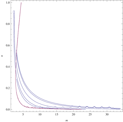
Figure 1: The contour plot of $n_{s}$ and $r$ for the range of values $n_{s}=[0.9635,0.968]$ and $r=0.055$, as functions of $m$ and $n$, with the latter taking values in the ranges $m=[2,34]$ and $n=[0,1]$, for $(N,\Lambda,\xi,c_{1})=(60,2\times 10^{-7},0.14,10^{20})$.

As a final task before ending this section, we shall investigate the values of the wave speed $c_{A}^{2}$, for the values of the free parameters for which the compatibility with the latest Planck data is obtained. Particularly, if $c_{A}^{2}<0$, then Jeans instabilities occur in the theory and also superluminal modes may occur if $c_{A}^{2}>1$ Babichev:2007dw . A thorough investigation of the parameter space shows that $0<c_{A}^{2}<1$ for a wide range of values, even for the values of the free parameters for which the model is not phenomenologically viable. For example, in the case $(N,\Lambda,\xi,c_{1},m,n)=(60,2\times 10^{-7},0.14,10^{20},30.1,10^{-5})$ for which the model is compatible with the Planck data, the wave speed is equal to $c_{A}^{2}=0.33333$. In order to have a clear picture of the behavior of the wave speed, in Fig. 2 we present the contour plot of the wave speed $c_{A}^{2}$ as a function of $\xi$ and $\Lambda$, for $(N,c_{1},m,n)=(60,10^{20},30.1,10^{-5})$ and for $\Lambda$ and $\xi$ chosen in the ranges $\Lambda=[0,10]$ and $\xi=[0,10]$. The darker contours indicate that the values of $c_{A}^{2}$ grow larger. As it can be seen, the wave speed takes in all cases values $0<c_{A}^{2}<1$, so neither Jeans instabilities nor superluminal modes occur in the theory.

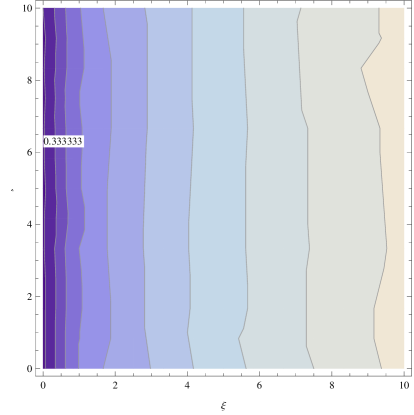
Figure 2: The contour plot of the wave speed $c_{A}^{2}$ as a function of $\xi$ and $\Lambda$, for $(N,c_{1},m,n)=(60,10^{20},30.1,10^{-5})$ and for $\Lambda$ and $\xi$ chosen in the ranges $\Lambda=[0,10]$ and $\xi=[0,10]$. Darker contours indicate larger values of $c_{A}^{2}$.

Finally, before closing this section we need to validate that the assumptions made in Eqs. (18) and (19) hold true, for the values of the free parameters that guarantee the viability of the model. Indeed by choosing, $(N,\Lambda,\xi,c_{1},m,n)=(60,2\times 10^{-7},0.14,10^{20},30.1,10^{-5})$, in reduced Planck units, the term $\Big{|}\frac{c_{1}\dot{\phi}^{4}}{2}\Big{|}$ reads,

$$\Big{|}\frac{c_{1}\dot{\phi}^{4}}{2}\Big{|}=6.11811\times 10^{-22}\,,$$ (37)

and the term $\Big{|}\frac{Hh^{\prime}(\phi)\dot{\phi}}{\kappa^{2}}\Big{|}$,

$$\Big{|}\frac{Hh^{\prime}(\phi)\dot{\phi}}{\kappa^{2}}\Big{|}=2.0326\times 10^{-28}\,,$$ (38)

while the term $\Big{|}\frac{h^{\prime\prime}(\phi)\dot{\phi}^{2}}{\kappa^{2}}\Big{|}$ is approximately,

$$\Big{|}\frac{h^{\prime\prime}(\phi)\dot{\phi}^{2}}{\kappa^{2}}\Big{|}=1.1\times 10^{-31}\,,$$ (39)

so obviously the assumptions in Eqs. (18) and (19) hold true. In addition, let us also validate that the assumption of Eq. (14) holds true, so by also using $(N,\Lambda,\xi,c_{1},m,n)=(60,2\times 10^{-7},0.14,10^{20},30.1,10^{-5})$, in reduced Planck units, we get,

$$V(\phi)=1.11093\times 10^{-19}$$ (40)

in reduced Planck units, which is obviously way larger than the numerical value appearing in Eq. (37). So we validated that the approximations we made for a slow-rolling scalar hold true. We need to note that the slow-roll assumptions in our case, and in contrast to the standard canonical scalar field case, invoke the derivatives of the scalar field and the coupling to the curvature scalar, namely the function $h(\phi)$.

II.2 Models with Potential: Constant-roll Phenomenology

Unlike in the slow-roll case, the model of Eq. (29) may become compatible with the latest Planck data, if the slow-roll assumption for the scalar field, namely Eq. (13) is replaced by the constant-roll assumption,

$$\ddot{\phi}=\beta H\dot{\phi}\,,$$ (41)

where $\beta$ is a dimensionless free parameter. Thus, in view of the constant-roll condition (41), and also by still assuming that the condition (14) holds true, the equations of motion for the model (12) yield the following solutions for $\dot{\phi}$, $H$ and $\dot{H}$ as a function of the scalar field,

$$H\simeq\frac{\sqrt{\frac{\kappa^{2}V(\phi)}{h(\phi)}}}{\sqrt{3}}\,,$$ (42)

$$\dot{H}\simeq-\frac{\text{c1}\kappa^{2}\left(\frac{2V^{\prime}(\phi)-\frac{4V(\phi)h^{\prime}(\phi)}{h(\phi)}}{(\beta+1)\text{c1}\sqrt{\frac{\kappa^{2}V(\phi)}{h(\phi)}}}\right)^{4/3}}{4\ 3^{2/3}h(\phi)}\,,$$ (43)

$$\dot{\phi}\simeq-\frac{\sqrt[3]{\frac{2V^{\prime}(\phi)-\frac{4V(\phi)h^{\prime}(\phi)}{h(\phi)}}{(\beta+1)\text{c1}\sqrt{\frac{\kappa^{2}V(\phi)}{h(\phi)}}}}}{\sqrt[6]{3}}\,.$$ (44)

Accordingly, the slow-roll indices (52) in terms of the scalar field and the free parameters of the theory, including $\beta$ in the case at hand, read,

$$\epsilon_{1}\simeq-\frac{\sqrt[3]{3}\text{c1}e^{\kappa\phi}\left((2\gamma+1)^{4/3}\Lambda e^{\frac{1}{3}4\gamma\kappa\phi}\left(\kappa^{4/3}\xi^{4/6}e^{\frac{1}{6}4(-(\gamma+1))\kappa\phi}\right)\right)}{\left(2^{2/3}\xi\right)\left(\Lambda^{4/6}\left(\kappa^{4/3}((\beta+1)\text{c1})^{4/3}\right)\right)}\,,$$ (45)

$$\epsilon_{2}\simeq\beta\,,$$

$$\epsilon_{3}\simeq\frac{h^{\prime}(\phi)\sqrt[3]{\frac{6V(\phi)h^{\prime}(\phi)-3h(\phi)V^{\prime}(\phi)}{(\beta+1)\text{c1}h(\phi)\sqrt{\frac{\kappa^{2}V(\phi)}{h(\phi)}}}}}{2^{2/3}h(\phi)\sqrt{\frac{\kappa^{2}V(\phi)}{h(\phi)}}}\,,$$

$$\epsilon_{4}\simeq\frac{\sqrt[3]{6}(\beta+1)h^{\prime}(\phi)\left(\frac{2V(\phi)h^{\prime}(\phi)-h(\phi)V^{\prime}(\phi)}{(\beta+1)\text{c1}h(\phi)\sqrt{\frac{\kappa^{2}V(\phi)}{h(\phi)}}}\right)^{2/3}\left(\text{c1}\kappa^{2}\left(\frac{2V(\phi)h^{\prime}(\phi)-h(\phi)V^{\prime}(\phi)}{(\beta+1)\text{c1}h(\phi)\sqrt{\frac{\kappa^{2}V(\phi)}{h(\phi)}}}\right)^{2/3}+\sqrt[3]{6}h^{\prime\prime}(\phi)\right)}{\sqrt[3]{6}(\beta+1)h^{\prime}(\phi)^{2}\sqrt{\frac{\kappa^{2}V(\phi)}{h(\phi)}}\sqrt[3]{\frac{2V(\phi)h^{\prime}(\phi)-h(\phi)V^{\prime}(\phi)}{(\beta+1)\text{c1}h(\phi)\sqrt{\frac{\kappa^{2}V(\phi)}{h(\phi)}}}}+4\kappa^{2}V(\phi)h^{\prime}(\phi)-2\kappa^{2}h(\phi)V^{\prime}(\phi)}\,.$$

Also in this case, the wave speed $c_{A}$ reads,

$$c_{A}=\sqrt{\frac{\frac{1}{2}3^{2/3}\gamma^{2}\Lambda e^{\gamma\kappa\phi}\left(\frac{-4\gamma\kappa\xi e^{-\kappa\phi}-2\kappa\xi e^{-\kappa\phi}}{(\beta+1)\text{c1}\sqrt{\frac{\kappa^{2}\xi e^{-\gamma\kappa\phi-\kappa\phi}}{\Lambda}}}\right)^{2/3}+\frac{\text{c1}\left(\frac{-4\gamma\kappa\xi e^{-\kappa\phi}-2\kappa\xi e^{-\kappa\phi}}{(\beta+1)\text{c1}\sqrt{\frac{\kappa^{2}\xi e^{-\gamma\kappa\phi-\kappa\phi}}{\Lambda}}}\right)^{4/3}}{2\ 3^{2/3}}}{\frac{1}{2}3^{2/3}\gamma^{2}\Lambda e^{\gamma\kappa\phi}\left(\frac{-4\gamma\kappa\xi e^{-\kappa\phi}-2\kappa\xi e^{-\kappa\phi}}{(\beta+1)\text{c1}\sqrt{\frac{\kappa^{2}\xi e^{-\gamma\kappa\phi-\kappa\phi}}{\Lambda}}}\right)^{2/3}+\frac{1}{2}\sqrt[3]{3}\text{c1}\left(\frac{-4\gamma\kappa\xi e^{-\kappa\phi}-2\kappa\xi e^{-\kappa\phi}}{(\beta+1)\text{c1}\sqrt{\frac{\kappa^{2}\xi e^{-\gamma\kappa\phi-\kappa\phi}}{\Lambda}}}\right)^{4/3}}}\,.$$ (46)

Following the same procedure as in the previous subsection, we may easily obtain the spectral index and the tensor-to-scalar ratio as a function of the $e$-foldings number $N$ and the free parameters of the theory, including $\beta$, for the model of Eq. (29). However the final expressions are too lengthy to quote here, so we directly proceed to the analysis of the phenomenological viability of the model. As in the slow-roll case, we shall work in reduced Planck units, so by choosing for example $(N,\Lambda,\xi,c_{1},\gamma,\beta)=(60,10^{-20},10^{-6},10^{40},10^{8},0.017)$, we obtain,

$$n_{s}=0.965999,\,\,\,r=3.00219\times 10^{-6}\,,$$ (47)

which are compatible with the Planck 2018 constraints (28). We need to note that the viability for the exponential model (29) comes with more difficulty in comparison to the power-law model (30), but this is a model-dependent feature and has nothing to do with the constant-roll condition. Finally, the wave speed is also between $0<c_{A}^{2}<1$, at least for the values of the free parameters that guarantee the phenomenological viability of the model, so no Jeans instabilities or superluminal propagation of scalar modes occur in this case too. For example, if we choose $(N,\Lambda,\xi,c_{1},\gamma,\beta)=(60,10^{-20},10^{-6},10^{40},10^{8},0.017)$, we have $c_{A}^{2}=0.333333$, which of course satisfies $0<c_{A}^{2}<1$.

Having discussed the models with potential, in the next subsection we proceed to the study of models of the form (3) without scalar potential.

II.3 Model without Potential: Standard and Constant-roll Evolution

Let us now consider another model of $k$-inflation, in this case without scalar potential. The model is of the form of non-minimally coupled scalar field to gravity, and with only the higher order kinetic term appearing in the Lagrangian. Particularly, the $f(R,X,\phi)$ function has the following form,

$$f(R,\phi,X)=\frac{h(\phi)R}{\kappa^{2}}+c_{1}X^{2}\,.$$ (48)

In this subsection we shall consider the phenomenology of the above model, with respect to its viability, in the constant-roll case.

We shall assume that the constant-roll condition of Eq. (41) holds true for the scalar field. The non-constant-roll case can be obtained easily by setting $\beta=0$ in the equations that will follow. In this case, without assuming any condition on the scalar field, except for the constant-roll evolution of Eq. (41), the expressions for $H$, $\dot{H}$ and $\dot{\phi}$ as functions of the scalar field, are,

$$H=\frac{32\sqrt{\frac{2}{15}}h^{\prime}(\phi)^{2}\sqrt{\frac{\text{c1}\kappa^{2}}{h(\phi)}}}{3(\beta+1)^{2}\text{c1}\kappa^{2}h(\phi)}\,,$$ (49)

$$\dot{H}\simeq\Big{(}\frac{Hh^{\prime}(\phi)\dot{\phi}}{\kappa^{2}}-\frac{h^{\prime\prime}(\phi)\dot{\phi}^{2}}{\kappa^{2}}-\frac{c_{1}\dot{\phi}^{4}}{2}\Big{)}\,,$$ (50)

$$\dot{\phi}=\frac{8\sqrt{\frac{2}{15}}h^{\prime}(\phi)}{(\beta+1)h(\phi)\sqrt{\frac{\text{c1}\kappa^{2}}{h(\phi)}}}\,,$$ (51)

and notice that the expressions for $\dot{H}$ given in Eqs. (16) and (50) coincide. The slow-roll indices (52) as functions of the scalar field $\phi$ for the model (48), can easily be evaluated by using equations (49), (50) and (51), so these read,

$$\epsilon_{1}=-\frac{2\phi^{-2n}\left(\text{c1}n+(\beta+1)\Lambda^{2}((4\beta+5)n-4(\beta+1))\phi^{2n}\right)}{\Lambda^{2}n}\,,$$ (52)

$$\epsilon_{2}=\beta\,,$$

$$\epsilon_{3}=-\frac{2(\beta+1)^{3}\phi^{2}\sqrt{\kappa^{2}\Lambda\phi^{n}}\sqrt{\frac{n^{4}\phi^{-n-4}}{(\beta+1)^{4}\kappa^{2}\Lambda}}}{n^{2}}\,,$$

$$\epsilon_{4}=-\frac{2n\left(\text{c1}n+4(\beta+1)^{2}\Lambda^{2}(n-1)\phi^{2n}\right)}{(\beta+1)\phi^{2}\sqrt{\kappa^{2}\Lambda\phi^{n}}\left(\text{c1}+2(\beta+1)^{2}\Lambda^{2}\phi^{2n}\right)\sqrt{\frac{n^{4}\phi^{-n-4}}{(\beta+1)^{4}\kappa^{2}\Lambda}}}\,.$$

We shall consider the model,

$$h(\phi)=\Lambda\phi^{n}\,,$$ (53)

which is similar with the case in the presence of a potential, so we now examine the viability of the present model. Also in this case, the wave speed $c_{A}$ of Eq. (7) reads,

$$c_{A}=\sqrt{\frac{\frac{\text{c1}n^{4}\phi^{-2n-4}}{8(\beta+1)^{4}\kappa^{4}\Lambda^{2}}+\frac{3n^{4}}{4(\beta+1)^{2}\kappa^{4}\phi^{4}}}{\frac{3\text{c1}n^{4}\phi^{-2n-4}}{8(\beta+1)^{4}\kappa^{4}\Lambda^{2}}+\frac{3n^{4}}{4(\beta+1)^{2}\kappa^{4}\phi^{4}}}}\,,$$ (54)

Using the $e$-foldings number, which in this case, the term $\frac{H}{\dot{\phi}}$ in Eq. (26) reads,

$$\frac{H}{\dot{\phi}}\simeq-\frac{h^{\prime}(\phi)}{4(\beta+1)h(\phi)}\,,$$ (55)

so the slow-roll indices, the corresponding observational indices and the wave speed, shall be evaluated for the following scalar field value $\phi$ at the horizon crossing,

$$\phi_{i}=2^{\frac{1}{2n}}\Lambda^{-1/n}\left(-\frac{\left(8\beta^{2}+18\beta+9\right)n-8(\beta+1)^{2}}{\text{c1}n}\right)^{-\frac{1}{2n}}e^{\frac{4(\beta+1)N}{n}}\,.$$ (56)

The resulting expression for the observational indices and the wave speed are quite lengthy to quote here, but a detailed analysis indicates that neither the constant-roll ($\beta\neq 0$) not the slow-roll case ($\beta=0$) case, yield any viable results. In fact, the spectral index can be compatible with the Planck data, however the tensor-to-scalar ratio is always extremely higher than the allowed observational data. However, the wave speed is always nearly equal to unity, for all the values of the free parameters that yield sensible results (non-imaginary values). Therefore, we may claim even from now that the power-law model without scalar potential is not so appealing.

We need to note that in the literature an interesting class of models is studied Li:2012vta , in which case a scalar potential and only a higher kinetic term is included in the Lagrangian, without a canonical kinetic term. These theories can be viable, and in contrast, the non-minimally coupled theory with only a higher kinetic term is not viable, at least when the non-minimally coupled function is a power-law type. Perhaps including higher order kinetic terms, higher than the quadratic which we studied, may resolve this issue, but we leave this to the reader, since it is a repetition of the method we provided above, and the result is highly model dependent, with the dependence quantified in the choice of the coupling function to the curvature scalar $h(\phi)$.

II.4 Conformally Transformed Models with Scalar Potential and Implications

The viability of the models with scalar potential of the form (12) has a direct implication for minimally coupled $k$-inflation models with non-trivial higher-order kinetic terms, with scalar potential, due to the fact that these two theories are related via a conformal transformation. From a phenomenological point of view, the power spectrum of the primordial scalar curvature perturbations and the power spectrum of the tensor perturbations are conformal invariant quantities, so the spectral index of the primordial curvature perturbations and the tensor-to-scalar ratio for the two theories are expected to be the same in principle, although deviations from this rule are presented in the literature, mainly related to the slow-roll condition Odintsov:2018qyy ; Karam:2019dlv ; Karam:2017zno . Let us consider the action of the non-minimally coupled $k$-inflation theory with scalar potential corresponding to Eq. (12), which is,

$$\mathcal{S}=\int d^{4}x\sqrt{-g}\left[\frac{1}{2}\left(\frac{h(\phi)R}{\kappa^{2}}-2V(\phi)+c_{1}\gamma X^{2}\right)\right]\,,$$ (57)

and let us perform a conformal transformation of the metric, which has the following form,

$$g_{\mu\nu}=\Omega^{-2}(x^{\mu})\tilde{g}_{\mu\nu}\,,$$ (58)

where $\Omega(x^{\mu})$ is a differentiable function of the spacetime coordinates, and the “tilde” metric denotes the conformally transformed metric. Accordingly, $\sqrt{-g}$ and $g^{\mu\nu}$ under the conformal transformation $\Omega(x^{\mu})$ transform as follows,

$$g^{\mu\nu}=\Omega(x^{\mu})\tilde{g}^{\mu\nu}\,,\,\,\,\sqrt{-g}=\Omega^{-4}\sqrt{-\tilde{g}}\,.$$ (59)

We introduce the notation,

$$f=\ln\Omega(x^{\mu})\,,\,\,\,f_{\mu}=\frac{\partial_{\mu}\Omega}{\Omega}=\partial_{\mu}f\,,$$ (60)

and therefore we have, $\tilde{f}^{\mu}=\tilde{g}^{\mu\nu}f_{\nu}$. Using the conformal transformation rules and the notation (60), the Ricci scalar under the conformal transformation, transforms as follows,

$$R=\Omega^{2}\left(\tilde{R}+6\tilde{\square}f-6\tilde{g}^{\mu\nu}f_{\mu}f_{\nu}\right)\,,$$ (61)

where the d’Alembertian is,

$$\tilde{\square}f=\frac{1}{\sqrt{-\tilde{g}}}\partial_{\mu}\left(\sqrt{-\tilde{g}}\tilde{g}^{\mu\nu}\partial_{\nu}f\right)\,.$$ (62)

Having the transformation properties at hand, we can conformally transform each term of the action (57) straightforwardly. The term $\sim h(\phi)R$ transforms as,

$$\frac{1}{2}\sqrt{-g}h(\phi)R\to\frac{1}{2}\sqrt{-\tilde{g}}h(\phi)\Omega^{-2}\left(\tilde{R}+6\tilde{\square}f-6\tilde{g}^{\mu\nu}f_{\mu}f_{\nu}\right)\,.$$ (63)

Without loss of generality, since $\Omega$ is arbitrary, we can choose,

$$h(\phi)\Omega^{-2}=1\,,$$ (64)

so it is obvious that with this choice, the conformally transformed frame becomes the Einstein frame due to the occurrence of the term $\sim\sqrt{-\tilde{g}}\tilde{R}$. The second term in the Einstein frame which is $\sim\tilde{\square}f$ is a total derivative, so it disappears by integrating, subject to the constraint that the integral of the function $f$ on the boundary of the spacetime vanishes. For the choice (64), we have,

$$f_{\mu}=\frac{1}{2}\frac{\partial_{\mu}h}{h}=\frac{h^{\prime}}{2h}\partial_{\mu}\phi\,,$$ (65)

where the “prime” indicates differentiation with respect to the scalar field. Hence, with the choice (64) in conjunction with (65), the transformation for the first term finally becomes,

$$\frac{1}{2}\sqrt{-g}h(\phi)R\to\frac{1}{2}\sqrt{-\tilde{g}}\left(\tilde{R}-\frac{3}{2}\left(\frac{h^{\prime}}{h}\right)^{2}\tilde{g}^{\mu\nu}\partial_{\mu}\phi\partial_{\nu}\phi\right)\,.$$ (66)

Accordingly, the potential term $\sim-2V(\phi)$ transforms as,

$$\frac{-\sqrt{-g}}{2}\left(-2V(\phi)\right)\to\frac{-\sqrt{-\tilde{g}}}{2}\frac{1}{h^{2}}\left(-2V(\phi)\right)\,,$$ (67)

and the higher order kinetic term $\sim c_{1}X^{2}$ transforms as,

$$\frac{\sqrt{-g}}{2}c_{1}X^{2}=\frac{\sqrt{-g}}{2}c_{1}\left(\frac{1}{2}g^{\mu\nu}\partial_{\mu}\phi\partial_{\nu}\phi\right)^{2}$$ (68)

$$=\frac{\sqrt{-\tilde{g}}}{2}\Omega^{-4}c_{1}\left(\frac{1}{2}\Omega^{2}\tilde{g}^{\mu\nu}\partial_{\mu}\phi\partial_{\nu}\phi\right)^{2}=\frac{\sqrt{-\tilde{g}}}{2}c_{1}\left(\frac{1}{2}\tilde{g}^{\mu\nu}\partial_{\mu}\phi\partial_{\nu}\phi\right)^{2}$$

$$=\frac{\sqrt{-\tilde{g}}}{2}c_{1}X^{2}\,,$$

so it is basically the same as in the Jordan frame. This result is an artifact of the choice $\mu=2$ in Eq. (3), and for a general $\mu$, the conformal transformation would read,

$$\frac{\sqrt{-g}}{2}c_{1}X^{\mu}=\frac{\sqrt{-g}}{2}c_{1}\left(\frac{1}{2}g^{\mu\nu}\partial_{\mu}\phi\partial_{\nu}\phi\right)^{\mu}$$ (69)

$$=\frac{\sqrt{-\tilde{g}}}{2}\Omega^{-4}c_{1}\left(\frac{1}{2}\Omega^{2}\tilde{g}^{\mu\nu}\partial_{\mu}\phi\partial_{\nu}\phi\right)^{\mu}=\frac{\sqrt{-\tilde{g}}}{2}c_{1}\left(\frac{1}{2}\tilde{g}^{\mu\nu}\partial_{\mu}\phi\partial_{\nu}\phi\right)^{\mu}$$

$$=\frac{\sqrt{-\tilde{g}}}{2}\Omega^{2(-2+\mu)}c_{1}X^{\mu}\,.$$

Therefore, the conformally transformed action (57) in the Einstein frame for general $\mu$ reads,

$$\mathcal{S}=\int d^{4}x\sqrt{-\tilde{g}}\frac{1}{2}\left[\tilde{R}-\frac{3}{2}\left(\frac{h^{\prime}}{h}\right)^{2}\tilde{g}^{\mu\nu}\partial_{\mu}\phi\partial_{\nu}\phi-\frac{2}{h^{2}}V(\phi)+h(\phi)^{(-2+\mu)}c_{1}X^{\mu}\right]\,.$$ (70)

The above action can easily be transformed to an Einstein frame scalar $k$-inflation theory with canonical kinetic term, by appropriately redefining the scalar field. Thus, due to the conformal relation between the actions (57) and (70), and owing to the fact that both the scalar and tensor power spectrum is conformal invariant, the two theories can produce similar phenomenology. This fact indicates that the model (70) with $\mu=2$ can be a viable model, and we can conclude this without performing the actual calculations, which would be more tedious in comparison to the model (57). Similar results can hold true for general $\mu$ but we do not present here for brevity.

III Conclusions

In this paper we studied in depth several $k$-inflation models with non-minimal coupling of the scalar field to the scalar curvature. We mainly focused on models that lack of a canonical kinetic term for the scalar field, in the presence and the absence of a scalar potential, and we studied two cases with regard to the evolution of the scalar field, the slow-roll and the constant-roll case. In the presence of a scalar potential, and with the higher order kinetic term being of the form $\sim c_{1}X^{2}$, when the slow-roll conditions are assumed for the scalar field, we demonstrated that a phenomenologically viable theory can be obtained. Particularly, we calculated the slow-roll indices and the observational indices and we showed that the results can be compatible with the latest Planck constraints. This result is of course model dependent, but it is quite general since it can hold true for several choices of the potential and the non-minimal coupling function $h(\phi)$. Also the sound speed of the model never exceeds unity for a wide range of the free parameters of the model, therefore no superluminal propagation occurs, and also it is positive and hence no instabilities occur. Similar results are obtained when the constant-roll condition is assumed for the model. In the case that the scalar potential is absent, the power-law model is not viable, however the results are model dependent, and perhaps the inclusion of higher order kinetic terms may render the model phenomenologically viable. Finally, we performed a conformal transformation of the non-minimally coupled $k$-inflation theory with potential, and the resulting Einstein frame theory contains a scalar potential, the higher-order kinetic term and an ordinary scalar kinetic term. Due to the conformal invariance of both the scalar and tensor power spectra, we argued that the resulting Einstein frame can also be viable and compatible with the observational data. The latter theory is quite more involved to handle analytically, thus by studying the non-minimally coupled model, one may obtain several phenomenological conclusions for the Einstein frame theory. Nevertheless, the most correct way to prove the equivalence is to calculate the observational indices, using the slow-roll or the constant-roll condition, due to the fact that the very slow-roll condition may obscure the equivalence of the two theories, see for example Odintsov:2018qyy ; Karam:2019dlv ; Karam:2017zno . This task is not easy in general though, but we hope to address it in a forthcoming work.

References

- (1) B. P. Abbott et al. “Multi-messenger Observations of a Binary Neutron Star Merger,” Astrophys. J. 848 (2017) no.2, L12 doi:10.3847/2041-8213/aa91c9 [arXiv:1710.05833 [astro-ph.HE]].
- (2) J. M. Ezquiaga and M. Zumalacarregui, Phys. Rev. Lett. 119 (2017) no.25, 251304 doi:10.1103/PhysRevLett.119.251304 [arXiv:1710.05901 [astro-ph.CO]].
- (3) S. Nojiri, S. D. Odintsov and V. K. Oikonomou, Phys. Rept. 692 (2017) 1 doi:10.1016/j.physrep.2017.06.001 [arXiv:1705.11098 [gr-qc]].
- (4) S. Nojiri and S. D. Odintsov, Phys. Rept. 505 (2011) 59 doi:10.1016/j.physrep.2011.04.001 [arXiv:1011.0544 [gr-qc]].
- (5) S. Nojiri and S. D. Odintsov, eConf C 0602061 (2006) 06 [Int. J. Geom. Meth. Mod. Phys. 4 (2007) 115] doi:10.1142/S0219887807001928 [hep-th/0601213].
- (6) S. Capozziello and M. De Laurentis, Phys. Rept. 509 (2011) 167 doi:10.1016/j.physrep.2011.09.003 [arXiv:1108.6266 [gr-qc]].
- (7) V. Faraoni and S. Capozziello, Fundam. Theor. Phys. 170 (2010). doi:10.1007/978-94-007-0165-6
- (8) A. de la Cruz-Dombriz and D. Saez-Gomez, Entropy 14 (2012) 1717 doi:10.3390/e14091717 [arXiv:1207.2663 [gr-qc]].
- (9) G. J. Olmo, Int. J. Mod. Phys. D 20 (2011) 413 doi:10.1142/S0218271811018925 [arXiv:1101.3864 [gr-qc]].
- (10) S. Nojiri and S. D. Odintsov, Phys. Rev. D 68 (2003) 123512 doi:10.1103/PhysRevD.68.123512 [hep-th/0307288].
- (11) C. Armendariz-Picon, T. Damour and V. F. Mukhanov, Phys. Lett. B 458 (1999) 209 doi:10.1016/S0370-2693(99)00603-6 [hep-th/9904075].
- (12) T. Chiba, T. Okabe and M. Yamaguchi, Phys. Rev. D 62 (2000) 023511 doi:10.1103/PhysRevD.62.023511 [astro-ph/9912463].
- (13) C. Armendariz-Picon, V. F. Mukhanov and P. J. Steinhardt, Phys. Rev. Lett. 85 (2000) 4438 doi:10.1103/PhysRevLett.85.4438 [astro-ph/0004134].
- (14) J. Matsumoto and S. Nojiri, Phys. Lett. B 687 (2010) 236 doi:10.1016/j.physletb.2010.03.030 [arXiv:1001.0220 [hep-th]].
- (15) C. Armendariz-Picon, V. F. Mukhanov and P. J. Steinhardt, Phys. Rev. D 63 (2001) 103510 doi:10.1103/PhysRevD.63.103510 [astro-ph/0006373].
- (16) T. Chiba, Phys. Rev. D 66 (2002) 063514 doi:10.1103/PhysRevD.66.063514 [astro-ph/0206298].
- (17) M. Malquarti, E. J. Copeland, A. R. Liddle and M. Trodden, Phys. Rev. D 67 (2003) 123503 doi:10.1103/PhysRevD.67.123503 [astro-ph/0302279].
- (18) M. Malquarti, E. J. Copeland and A. R. Liddle, Phys. Rev. D 68 (2003) 023512 doi:10.1103/PhysRevD.68.023512 [astro-ph/0304277].
- (19) L. P. Chimento and A. Feinstein, Mod. Phys. Lett. A 19 (2004) 761 doi:10.1142/S0217732304013507 [astro-ph/0305007].
- (20) L. P. Chimento, Phys. Rev. D 69 (2004) 123517 doi:10.1103/PhysRevD.69.123517 [astro-ph/0311613].
- (21) R. J. Scherrer, Phys. Rev. Lett. 93 (2004) 011301 doi:10.1103/PhysRevLett.93.011301 [astro-ph/0402316].
- (22) J. M. Aguirregabiria, L. P. Chimento and R. Lazkoz, Phys. Rev. D 70 (2004) 023509 doi:10.1103/PhysRevD.70.023509 [astro-ph/0403157].
- (23) C. Armendariz-Picon and E. A. Lim, JCAP 0508 (2005) 007 doi:10.1088/1475-7516/2005/08/007 [astro-ph/0505207].
- (24) L. R. Abramo and N. Pinto-Neto, Phys. Rev. D 73 (2006) 063522 doi:10.1103/PhysRevD.73.063522 [astro-ph/0511562].
- (25) A. D. Rendall, Class. Quant. Grav. 23 (2006) 1557 doi:10.1088/0264-9381/23/5/008 [gr-qc/0511158].
- (26) J. P. Bruneton, Phys. Rev. D 75 (2007) 085013 doi:10.1103/PhysRevD.75.085013 [gr-qc/0607055].
- (27) R. de Putter and E. V. Linder, Astropart. Phys. 28 (2007) 263 doi:10.1016/j.astropartphys.2007.05.011 [arXiv:0705.0400 [astro-ph]].
- (28) E. Babichev, V. Mukhanov and A. Vikman, JHEP 0802 (2008) 101 doi:10.1088/1126-6708/2008/02/101 [arXiv:0708.0561 [hep-th]].
- (29) C. Deffayet, X. Gao, D. A. Steer and G. Zahariade, Phys. Rev. D 84 (2011) 064039 doi:10.1103/PhysRevD.84.064039 [arXiv:1103.3260 [hep-th]].
- (30) N. Kan, K. Shiraishi and M. Yashiki, arXiv:1811.11967 [gr-qc].
- (31) S. Unnikrishnan, V. Sahni and A. Toporensky, JCAP 1208 (2012) 018 doi:10.1088/1475-7516/2012/08/018 [arXiv:1205.0786 [astro-ph.CO]].
- (32) S. Li and A. R. Liddle, JCAP 1210 (2012) 011 doi:10.1088/1475-7516/2012/10/011 [arXiv:1204.6214 [astro-ph.CO]].
- (33) I. D. Gialamas and A. B. Lahanas, arXiv:1911.11513 [gr-qc].
- (34) Y. Akrami et al. [Planck Collaboration], arXiv:1807.06211 [astro-ph.CO].
- (35) A. H. Guth, Phys. Rev. D 23 (1981) 347. doi:10.1103/PhysRevD.23.347
- (36) A. A. Starobinsky, Phys. Lett. 91B (1980) 99. doi:10.1016/0370-2693(80)90670-X
- (37) A. D. Linde, Phys. Lett. 129B (1983) 177. doi:10.1016/0370-2693(83)90837-7
- (38) A. Albrecht and P. J. Steinhardt, Phys. Rev. Lett. 48 (1982) 1220 [Adv. Ser. Astrophys. Cosmol. 3 (1987) 158]. doi:10.1103/PhysRevLett.48.1220
- (39) S. Inoue and J. Yokoyama, Phys. Lett. B 524 (2002) 15 doi:10.1016/S0370-2693(01)01369-7 [hep-ph/0104083].
- (40) N. C. Tsamis and R. P. Woodard, Phys. Rev. D 69 (2004) 084005 doi:10.1103/PhysRevD.69.084005 [astro-ph/0307463].
- (41) W. H. Kinney, Phys. Rev. D 72 (2005) 023515 doi:10.1103/PhysRevD.72.023515 [gr-qc/0503017].
- (42) K. Tzirakis and W. H. Kinney, Phys. Rev. D 75 (2007) 123510 doi:10.1103/PhysRevD.75.123510 [astro-ph/0701432].
- (43) M. H. Namjoo, H. Firouzjahi and M. Sasaki, Europhys. Lett. 101 (2013) 39001 doi:10.1209/0295-5075/101/39001 [arXiv:1210.3692 [astro-ph.CO]].
- (44) J. Martin, H. Motohashi and T. Suyama, Phys. Rev. D 87 (2013) no.2, 023514 doi:10.1103/PhysRevD.87.023514 [arXiv:1211.0083 [astro-ph.CO]].
- (45) H. Motohashi, A. A. Starobinsky and J. Yokoyama, JCAP 1509 (2015) no.09, 018 doi:10.1088/1475-7516/2015/09/018 [arXiv:1411.5021 [astro-ph.CO]].
- (46) Y. F. Cai, J. O. Gong, D. G. Wang and Z. Wang, JCAP 1610 (2016) no.10, 017 doi:10.1088/1475-7516/2016/10/017 [arXiv:1607.07872 [astro-ph.CO]].
- (47) H. Motohashi and A. A. Starobinsky, arXiv:1702.05847 [astro-ph.CO].
- (48) S. Hirano, T. Kobayashi and S. Yokoyama, Phys. Rev. D 94 (2016) no.10, 103515 doi:10.1103/PhysRevD.94.103515 [arXiv:1604.00141 [astro-ph.CO]].
- (49) L. Anguelova, Nucl. Phys. B 911 (2016) 480 doi:10.1016/j.nuclphysb.2016.08.020 [arXiv:1512.08556 [hep-th]].
- (50) J. L. Cook and L. M. Krauss, JCAP 1603 (2016) no.03, 028 doi:10.1088/1475-7516/2016/03/028 [arXiv:1508.03647 [astro-ph.CO]].
- (51) K. S. Kumar, J. Marto, P. Vargas Moniz and S. Das, JCAP 1604 (2016) no.04, 005 doi:10.1088/1475-7516/2016/04/005 [arXiv:1506.05366 [gr-qc]].
- (52) S. D. Odintsov and V. K. Oikonomou, arXiv:1703.02853 [gr-qc].
- (53) S. D. Odintsov and V. K. Oikonomou, arXiv:1704.02931 [gr-qc].
- (54) J. Lin, Q. Gao and Y. Gong, Mon. Not. Roy. Astron. Soc. 459 (2016) no.4, 4029 doi:10.1093/mnras/stw915 [arXiv:1508.07145 [gr-qc]].
- (55) Q. Gao and Y. Gong, arXiv:1703.02220 [gr-qc].
- (56) S. Nojiri, S. D. Odintsov and V. K. Oikonomou, Class. Quant. Grav. 34 (2017) no.24, 245012 doi:10.1088/1361-6382/aa92a4 [arXiv:1704.05945 [gr-qc]].
- (57) V. K. Oikonomou, Mod. Phys. Lett. A 32 (2017) no.33, 1750172 doi:10.1142/S0217732317501723 [arXiv:1706.00507 [gr-qc]].
- (58) S. D. Odintsov, V. K. Oikonomou and L. Sebastiani, Nucl. Phys. B 923 (2017) 608 doi:10.1016/j.nuclphysb.2017.08.018 [arXiv:1708.08346 [gr-qc]].
- (59) V. K. Oikonomou, Int. J. Mod. Phys. D 27 (2017) no.02, 1850009 doi:10.1142/S0218271818500098 [arXiv:1709.02986 [gr-qc]].
- (60) F. Cicciarella, J. Mabillard and M. Pieroni, JCAP 1801 (2018) no.01, 024 doi:10.1088/1475-7516/2018/01/024 [arXiv:1709.03527 [astro-ph.CO]].
- (61) A. Awad, W. El Hanafy, G. G. L. Nashed, S. D. Odintsov and V. K. Oikonomou, JCAP 1807 (2018) no.07, 026 doi:10.1088/1475-7516/2018/07/026 [arXiv:1710.00682 [gr-qc]].
- (62) L. Anguelova, P. Suranyi and L. C. R. Wijewardhana, JCAP 1802 (2018) no.02, 004 doi:10.1088/1475-7516/2018/02/004 [arXiv:1710.06989 [hep-th]].
- (63) A. Ito and J. Soda, Eur. Phys. J. C 78 (2018) no.1, 55 doi:10.1140/epjc/s10052-018-5534-5 [arXiv:1710.09701 [hep-th]].
- (64) A. Karam, L. Marzola, T. Pappas, A. Racioppi and K. Tamvakis, JCAP 1805 (2018) no.05, 011 doi:10.1088/1475-7516/2018/05/011 [arXiv:1711.09861 [astro-ph.CO]].
- (65) Z. Yi and Y. Gong, JCAP 1803 (2018) no.03, 052 doi:10.1088/1475-7516/2018/03/052 [arXiv:1712.07478 [gr-qc]].
- (66) A. Mohammadi, K. Saaidi and T. Golanbari, Phys. Rev. D 97 (2018) no.8, 083006 doi:10.1103/PhysRevD.97.083006 [arXiv:1801.03487 [hep-ph]].
- (67) Q. Gao, Y. Gong and Q. Fei, JCAP 1805 (2018) no.05, 005 doi:10.1088/1475-7516/2018/05/005 [arXiv:1801.09208 [gr-qc]].
- (68) A. Mohammadi and K. Saaidi, arXiv:1803.01715 [astro-ph.CO].
- (69) M. J. P. Morse and W. H. Kinney, Phys. Rev. D 97 (2018) no.12, 123519 doi:10.1103/PhysRevD.97.123519 [arXiv:1804.01927 [astro-ph.CO]].
- (70) D. Cruces, C. Germani and T. Prokopec, JCAP 1903 (2019) no.03, 048 doi:10.1088/1475-7516/2019/03/048 [arXiv:1807.09057 [gr-qc]].
- (71) J. T. Galvez Ghersi, A. Zucca and A. V. Frolov, JCAP 1905 (2019) no.05, 030 doi:10.1088/1475-7516/2019/05/030 [arXiv:1808.01325 [astro-ph.CO]].
- (72) B. Boisseau and H. Giacomini, arXiv:1809.09169 [gr-qc].
- (73) Q. Gao, Y. Gong and Z. Yi, arXiv:1901.04646 [gr-qc].
- (74) W. C. Lin, M. J. P. Morse and W. H. Kinney, arXiv:1904.06289 [astro-ph.CO].
- (75) A. Mohammadi, T. Golanbari and K. Saaidi, arXiv:1912.07006 [gr-qc].
- (76) H. Noh and J. c. Hwang, Phys. Lett. B 515 (2001) 231 doi:10.1016/S0370-2693(01)00875-9 [astro-ph/0107069].
- (77) J. c. Hwang and H. Noh, Phys. Rev. D 71 (2005) 063536 doi:10.1103/PhysRevD.71.063536 [gr-qc/0412126].
- (78) J. c. Hwang and H. Noh, Phys. Rev. D 66 (2002) 084009 doi:10.1103/PhysRevD.66.084009 [hep-th/0206100].
- (79) D. I. Kaiser and E. I. Sfakianakis, Phys. Rev. Lett. 112 (2014) no.1, 011302 doi:10.1103/PhysRevLett.112.011302 [arXiv:1304.0363 [astro-ph.CO]].
- (80) S. D. Odintsov and V. K. Oikonomou, Phys. Rev. D 97 (2018) no.6, 064005 doi:10.1103/PhysRevD.97.064005 [arXiv:1802.06486 [gr-qc]].
- (81) A. Karam, T. Pappas and K. Tamvakis, PoS CORFU 2018 (2019) 064 doi:10.22323/1.347.0064 [arXiv:1903.03548 [gr-qc]].
- (82) A. Karam, T. Pappas and K. Tamvakis, Phys. Rev. D 96 (2017) no.6, 064036 doi:10.1103/PhysRevD.96.064036 [arXiv:1707.00984 [gr-qc]].