CHEOPS observations of the HD 108236 planetary system: A fifth planet, improved ephemerides, and planetary radii

Abstract

Context. The detection of a super-Earth and three mini-Neptunes transiting the bright ($V$ = 9.2 mag) star HD 108236 (also known as TOI-1233) was recently reported on the basis of TESS and ground-based light curves.

Aims. We perform a first characterisation of the HD 108236 planetary system through high-precision CHEOPS photometry and improve the transit ephemerides and system parameters.

Methods. We characterise the host star through spectroscopic analysis and derive the radius with the infrared flux method. We constrain the stellar mass and age by combining the results obtained from two sets of stellar evolutionary tracks. We analyse the available TESS light curves and one CHEOPS transit light curve for each known planet in the system.

Results. We find that HD 108236 is a Sun-like star with $R_{\star}=0.877\pm 0.008\,R_{\odot}$, $M_{\star}=0.869^{+0.050}_{-0.048}\,M_{\odot}$, and an age of $6.7_{-5.1}^{+4.0}$ Gyr. We report the serendipitous detection of an additional planet, HD 108236 f, in one of the CHEOPS light curves. For this planet, the combined analysis of the TESS and CHEOPS light curves leads to a tentative orbital period of about 29.5 days. From the light curve analysis, we obtain radii of $1.615\pm 0.051$, $2.071\pm 0.052$, $2.539_{-0.065}^{+0.062}$, $3.083\pm 0.052$, and $2.017_{-0.057}^{+0.052}$ $R_{\oplus}$ for planets HD 108236 b to HD 108236 f, respectively. These values are in agreement with previous TESS-based estimates, but with an improved precision of about a factor of two. We perform a stability analysis of the system, concluding that the planetary orbits most likely have eccentricities smaller than 0.1. We also employ a planetary atmospheric evolution framework to constrain the masses of the five planets, concluding that HD 108236 b and HD 108236 c should have an Earth-like density, while the outer planets should host a low mean molecular weight envelope.

Conclusions. The detection of the fifth planet makes HD 108236 the third system brighter than $V$ = 10 mag to host more than four transiting planets. The longer time span enables us to significantly improve the orbital ephemerides such that the uncertainty on the transit times will be of the order of minutes for the years to come. A comparison of the results obtained from the TESS and CHEOPS light curves indicates that for a $V$ $\sim$ 9 mag solar-like star and a transit signal of $\sim$500 ppm, one CHEOPS transit light curve ensures the same level of photometric precision as eight TESS transits combined, although this conclusion depends on the length and position of the gaps in the light curve.

1 Introduction

Transiting exoplanets provide the unique opportunity to thoroughly characterise planetary systems, from atmospheres to orbital dynamics, and transiting multi-planet systems play a special role. Multi-planet systems enable one, for example, to identify the presence of orbital resonances among the detected planets in a system, giving the possibility to use transit timing variations (TTVs) to measure planetary masses and/or detect other planets in the system (e.g. Miralda-Escudé, 2002; Holman & Murray, 2005; Agol et al., 2005).

There are many additional reasons why multi-planet systems are of particular interest. The existence of multiple planets that formed in the same disk places stronger constraints on formation models relative to planets in isolation, motivating the quantification of orbital spacings, correlations and differences within a system (Lissauer et al., 2011; Fabrycky et al., 2014; Winn & Fabrycky, 2015; Weiss et al., 2018), and inspiring novel approaches to classification and statistical description (Alibert, 2019; Sandford et al., 2019; Gilbert & Fabrycky, 2020). The spacing of planets relative to mean motion resonances provides information about planetary migration during formation, as well as later tidal effects on orbits (Delisle et al., 2012; Izidoro et al., 2017). A system’s multiplicity is affected after formation by long-term orbital dynamics, whether driven internally or as a result of more distant undetected planetary perturbers (Pu & Wu, 2015; Mustill et al., 2017; He et al., 2020). Changes to orbits can even affect the climate of planets (Spiegel et al., 2010). Given that our own Solar System contains multiple planets, this all helps us to understand points of similarity and divergence between our system and others.

Multi-planet systems also offer the opportunity to study the correlation between the composition (bulk and/or atmospheric) of planets and their periods or equilibrium temperatures, particularly when both planetary masses and radii have been measured. This correlation is a powerful constraint on planet formation and composition models as the number of degrees of freedom one can play with in models is reduced by the fact that all planets formed in the same protoplanetary disk. However, observing such a correlation requires precise transit measurements and dynamical analyses (to assess mass values via TTVs or radial velocity follow-up), which in turn can be more easily done once precise ephemerides of the different planets in the system are known.

Finally, multi-planet systems are ideal laboratories for studying the evolution of planetary atmospheres. This process is controlled by the host star’s evolution (i.e. evolution of the stellar radius, mass, and high-energy radiation), by the physical characteristics of each planet (e.g. planetary mass, radius, and initial atmospheric mass fraction and composition), and by the orbital evolution of each planet. Within multi-planet systems, each planet evolved in its own way as a result of its specific planetary and orbital characteristics, but the range of possible evolutionary paths is limited by the fact that all planets in the system orbit the same star. This enables one not only to constrain the evolution history of the planets, but also aspects of the host star that would be unattainable otherwise, such as the evolution of the stellar rotation rate (e.g. Kubyshkina et al., 2019a, b; Owen & Campos Estrada, 2020).

The majority of transiting multi-planet systems known to date were detected by the Kepler and K2 missions (e.g. Coughlin et al., 2016; Mayo et al., 2018). Among these, about 60 systems host four or more transiting planets, but only two have a host star brighter than $V$ = 10 mag (Kepler-444: Campante et al. 2015; HIP 41378: Vanderburg et al. 2016). The launches of the TESS (Transiting Exoplanet Survey Satellite; Ricker et al., 2015) and CHEOPS (CHaracterising ExOPlanets Satellite; Benz et al., 2020) satellites have shifted the focus of the detection and characterisation of multi-planet systems towards brighter stars. While TESS, similarly to Kepler and K2, has a wide field of view (FoV) that is optimised for the detection of a large number of transiting planets, CHEOPS is a targeted mission, observing one system at a time to perform a precise characterisation.

As of 19 November 2020, TESS had discovered 82 confirmed planets and $\sim$ 60% of them belong to multi-planet systems. A non-exhaustive list of the multi-planet systems discovered by TESS includes HD 15337 (Gandolfi et al., 2019), TOI-125 (Quinn et al., 2019), HD 21749 (Dragomir et al., 2019), HR 858 (Vanderburg et al., 2019), LP 791-18 (Crossfield et al., 2019), L98-59 (Kostov et al., 2019), TOI-421 (Carleo et al., 2020), HD 63433 (Mann et al., 2020), and TOI-700 (Gilbert et al., 2020). Following the completion of its prime mission on 5 July 2020, TESS was extended for a further 27 months. This will not only allow us to re-observe many of the targets already studied during the prime mission to better characterise them, but also to observe additional stars for the first time.

Daylan et al. (2020, D20 hereafter) announced the detection with TESS of four transiting planets orbiting the bright ($V$ = 9.2 mag) solar-like star HD 108236. The four planets have periods of about 3.8, 6.2, 14.2, and 19.6 days. The radius of the innermost planet ($\approx$1.6 $R_{\oplus}$) suggests that this is possibly a rocky super-Earth, while the larger radii of the three outer planets ($\approx$2.1, 2.7, and 3.1 $R_{\oplus}$) indicate that they may still host a lightweight gaseous envelope (Fulton et al., 2017; Owen & Wu, 2017; Jin & Mordasini, 2018). From the TESS measurements, it follows that the inner planet lies inside the radius gap (Fulton et al., 2017), while the three larger outer planets are located around the peak comprising planets with a gaseous envelope, hence making this system of particular interest for atmospheric evolution studies.

D20 performed orbital dynamic simulations that showed that the system is stable, though a significant exchange of angular momentum among the planets in the system likely occurred. Furthermore, on the basis of these simulations, D20 suggested the possible presence of a fifth planet in the system with a period of 10.9 days. However, a dedicated analysis of the TESS light curve (LC) did not give definitive proof. Finally, the bright host star makes the HD 108236 system a primary target for planetary mass measurements through radial velocities (RVs) and for constraining the atmospheric properties of multi-planet systems (D20).

We report here the results obtained from CHEOPS high-precision photometric observations of one transit of each detected planet composing the HD 108236 system, taken almost one year after the TESS observations. The main goals of the observations presented here were to secure the ephemerides of all detected planets, to employ the exquisite quality of CHEOPS photometry to provide a first refinement of the system’s main properties, and to confirm or disprove the presence of the putative fifth planet at the approximately 10.9 days indicated by D20.

This paper is organised as follows. Section 2 presents the host star properties, and Section 3 describes the CHEOPS and TESS LCs. The data analysis is presented in Section 4, and results are reported in Section 5. Section 6 summarises the work and presents our conclusions.

2 Host star properties

HD 108236 is a bright Sun-like star (spectral type G3V) that is also known as HIP 60689, TOI-1233, and Gaia DR2 6125644402384918784. Between 13 December 2019 and 23 January 2020 (UT) we acquired 13 high-resolution spectra ($R$ = 115 000) of HD 108236 (programme ID 1102.C-0923, PI: Gandolfi) using the High Accuracy Radial velocity Planet Searcher (HARPS, Mayor et al., 2003) spectrograph mounted at the ESO-3.6 m telescope of La Silla Observatory, Chile. We set the exposure time to T_exp = 1100–1500 s depending on the sky and seeing conditions, which led to an average signal to noise ratio (S/N) per pixel of $\sim$100 at 550 nm. We used the co-added HARPS spectrum – which has a consequent S/N $\sim$ 360 per pixel – to derive the fundamental photospheric parameters of the star, namely, the effective temperature $T_{\mathrm{eff}}$, surface gravity $\log{g}$, and metal content [Fe/H]. We obtained $T_{\mathrm{eff}}=5660\pm 61$ K, $\log{g}=4.49\pm 0.11$, and [Fe/H]$=-0.28\pm 0.04$ dex, from spectral analysis, which made use of the ARES+MOOG tools (Sousa, 2014). In short, we measured the equivalent widths of iron lines using the ARES code (Sousa et al., 2007, 2015) on the combined HARPS spectrum. In this step, we used the list of iron lines presented in Sousa et al. (2008). The best fitting atmospheric parameters were obtained looking for convergence of both ionisation and excitation equilibria. For this step, we made use of a grid of Kurucz model atmospheres (Kurucz, 1993) and the radiative transfer code MOOG (Sneden, 1973). We also analysed the same spectra using the ’spectroscopy made easy’ (SME) code (Piskunov & Valenti, 2017), which uses a different method and a different grid of models (atlas12, Kurucz, 2013) achieving results well within 1 sigma of those obtained employing ARES+MOOG.

It has been suggested that individual abundances of heavy elements and specific elemental ratios end up controlling the structure and composition of the planets (e.g. Bond et al., 2010; Thiabaud et al., 2015; Unterborn et al., 2016; Santos et al., 2015). In particular, Mg/Si and Fe/Si mineralogical ratios were proposed as probes to constrain the internal structure of terrestrial planets (e.g. Dorn et al., 2015). Therefore, we specifically derived the abundances of Mg and Si using the same tools and models as for the atmospheric parameter determination, as well as using the classical curve-of-growth analysis method assuming local thermodynamic equilibrium. For deriving the abundances, we closely followed the methods described in Adibekyan et al. (2012) and Adibekyan et al. (2015). The solar reference Mg and Si abundances are taken from (Asplund et al., 2009). The Mg/Si and Fe/Si abundance ratios were calculated as

$$A/B=N_{A}/N_{B}=10^{\log\epsilon(A)}/10^{\log\epsilon(B)}\,,$$ (1)

where $N_{A}$ and $N_{B}$ represent the number of atoms of elements A and B, respectively, scaled assuming a hydrogen content of $10^{12}$ atoms, while $\log\epsilon(A)$ and $\log\epsilon(B)$ are the respective absolute elemental abundances (total number of atoms) expressed in logarithmic scale.

We employed the infrared flux method (IRFM; Blackwell & Shallis 1977) to calculate the radius of the host star through the determination of the stellar angular diameter $\theta$ and effective temperature using known relationships between these properties, optical and infrared broadband fluxes, and synthetic photometry obtained from stellar atmospheric models (Castelli & Kurucz, 2003) over various standard bandpasses. The Gaia G, G_BP, and G_RP, the 2MASS J, H, and K, and the WISE W1 and W2 fluxes and relative uncertainties were retrieved from the most recent data releases (Gaia Collaboration et al., 2018; Skrutskie et al., 2006; Wright et al., 2010, respectively). We applied a Markov chain Monte Carlo (MCMC) approach, setting priors on the stellar parameters taken from the spectroscopic analysis detailed above. Within this framework, accounting for the reddening $E(B-V)$, we compared the observed photometry with the synthetic one obtained from convolving stellar synthetic spectral energy distributions from the atlas Catalogues (Castelli & Kurucz, 2003) with the throughput of the considered photometric bands. From this analysis, we determined the stellar radius and $E(B-V)$ to be $R_{\mathrm{IRFM},\star}=0.877\pm 0.008\,R_{\odot}$ and $E(B-V)_{\rm IRFM}=0.12\pm 0.09$, respectively. These values are in agreement with those provided in the literature (D20), but have a precision on the stellar radius of twice that previously reported.

The stellar mass $M_{\star}$ and age $t_{\star}$ were inferred from evolutionary models. To obtain more robust results, we considered two different sets of tracks and isochrones: one set generated from the PARSEC v1.2S code (Marigo et al., 2017) and another with the CLES code (Code Liègeois d’Évolution Stellaire; Scuflaire et al., 2008). The two models differ for example in terms of solar mixture, helium-to-metal enrichment ratio, adopted reaction rates, and opacity and overshooting treatment. The PARSEC models adopt the solar-scaled composition given by Caffau et al. (2011), while the CLES models consider that given by Asplund et al. (2009). In PARSEC, the helium content $Y$ is assumed to increase with $Z$ according to a linear relation of the form $Y=\frac{\Delta Y}{\Delta Z}Z+Y_{p}$, where $\frac{\Delta Y}{\Delta Z}=1.78$ has been inferred from solar calibration and $Y_{p}=0.2485$ is the primordial helium abundance (Komatsu et al., 2011); instead, in CLES the helium content may vary regardless of the heavy elements abundances, or be fixed following a metal enrichment linear law as above. The PARSEC models have been computed considering the nuclear reaction rates given by the JINA REACLIB database (Cyburt et al., 2010), while the CLES models consider the compilation from Adelberger et al. (2011). For hot stars, PARSEC models use the opacities based on the Opacity Project (OP, Seaton, 2005), while CLES models consider the OPAL tables of opacities (Iglesias & Rogers, 1996); in the low-temperature regime, PARSEC complements its opacity database with ÆSOPUS opacities (Marigo & Aringer, 2009), while CLES with the opacities taken from Ferguson et al. (2005). Finally, the differences on the treatment of overshooting can be identified by comparing the relative descriptions in Bressan et al. (2012) for the PARSEC models and Scuflaire et al. (2008) for the CLES models.

To assess the discrepancies arising from the use of the two different stellar evolutionary models, we analysed a wide sample of CHEOPS targets with the isochrone placement technique presented in Bonfanti et al. (2015, 2016) considering both sets of isochrones and tracks. We calculated that differences in age and mass may amount to $\sim$20% and $\sim$4%, respectively. Therefore, we considered these values as a reference estimate for the internal precision of the isochrones.

Then, we specifically analysed HD 108236 to retrieve its mass $M_{\star}$ and age $t_{\star}$. The adopted input parameters were the $T_{\mathrm{eff}}$, [Fe/H], and stellar radius $R_{\mathrm{IRFM},\star}$. Two independent analyses were carried out considering both PARSEC and CLES evolutionary models. The first analysis used the Isochrone placement technique and its interpolating capability applied to pre-computed PARSEC grids of isochrones and tracks to derive the set of stellar masses ($M_{\star,1}\pm\Delta M_{\star,1}$) and ages ($t_{\star,1}\pm\Delta t_{\star,1}$) that best match the input parameters. The second analysis, instead, was performed by directly fitting the input parameters to the CLES stellar models to infer $M_{\star,2}\pm\Delta M_{\star,2}$ and $t_{\star,2}\pm\Delta t_{\star,2}$. To account for model-related uncertainties, we added in quadrature an uncertainty of 20% in age and of 4% in mass to the estimates obtained from each set of models. The values obtained from each of the two analyses are listed in Table 1.

From these values we built the corresponding Gaussian probability density functions to then obtain the final estimates of both mass and age. To avoid underestimating the final uncertainties, for each parameter we summed the two Gaussian distributions representing the outputs of the PARSEC and CLES analyses. The median of the combined distribution was assumed as our reference final value, and its corresponding error bars were inferred from the 15.87^th and 84.14^th percentile of the combined distribution, in order to provide the 1$\sigma$ (68.3%) standard confidence interval. At the end, we obtained $M_{\star}=0.869_{-0.048}^{+0.050}\,M_{\odot}$ and $t_{\star}=6.7_{-5.1}^{+4.0}$ Gyr, as final values for the stellar mass and age, respectively.

Table 1: Stellar mass and age values computed considering the PARSEC and CLES models. Their weighted average consistence has been successfully checked through the $p$-value criterion based on $\chi^{2}$ tests (see text for details).

Parameter		PARSEC	CLES	$p$-value
$M_{\star}$	[$M_{\odot}$]	$0.853\pm 0.043$	$0.886\pm 0.049$	0.61
$t_{\star}$	[Gyr]	$7.7\pm 3.1$	$4.7\pm 5.8$	0.62

Then we applied a $\chi^{2}$-test to identify whether results coming from the two different methods (i.e. PARSEC vs CLES) are consistent (null hypothesis), so to check whether their synthesis into single values is indeed a signal of the robustness of the results, rather than a mathematical artefact. To this end, we computed

$$\bar{\chi}^{2}=\displaystyle\sum_{i=1}^{2}\frac{(x_{i}-\bar{x})^{2}}{\sigma_{i}^{2}}\,,$$ (2)

where $x$ denotes the generic variable (either $M_{\star}$ or $t_{\star}$), $\sigma$ its uncertainty, and $\bar{x}$ the median value of the parameter of interest inferred from the combined distribution. We expect $\bar{\chi}^{2}$ to be drawn from a chi-square distribution $f(\chi_{\nu}^{2})$ with $\nu=2-1=1$ degrees of freedom as $\bar{x}$ depends on $x_{1}$ and $x_{2}$. Testing the null hypothesis, namely verifying whether the median of the combined distribution properly describes the data, means comparing the $\bar{\chi}^{2}$ value obtained from Equation (2) to a reference $\chi_{\alpha}^{2}$ value defined by

$$\int_{\chi_{\alpha}^{2}}^{+\infty}f(\chi^{2})\mathrm{d}\chi^{2}=\alpha\,,$$ (3)

where $\alpha$ is the adopted significance level, which we set equal to 0.05. If $\bar{\chi}^{2}>\chi_{\alpha}^{2}$, then we are $100(1-\alpha)\%=95\%$ confident that the null hypothesis is false; otherwise, the null hypothesis is confirmed when

$$\bar{\chi}^{2}<\chi_{\alpha}^{2}\Leftrightarrow p\mathrm{-value}>\alpha\,,$$ (4)

where

$$p\mathrm{-value}=\int_{\bar{\chi}^{2}}^{+\infty}f(\chi^{2})\mathrm{d}\chi^{2}\,.$$ (5)

These calculations (see $p$-values in Table 1) confirm that the two independent derivations of the stellar mass and age are consistent, implying that the median of the combined distribution can be used to assess $M_{\star}$ and $t_{\star}$ from our two sets of measurements. Table 2 lists the final adopted stellar parameters.

D20 also derived the stellar fundamental parameters, but employing different approaches: they started either from high-resolution spectroscopy or broad-band photometry to obtain different pairs of ($R_{\star}$, $M_{\star}$). All obtained values agree with our estimates within 1$\sigma$, except for the $M_{\star}$ value that they computed from the mass-radius relation of Torres et al. (2010), which is in any case $\sim$2$\sigma$ away also from the other $M_{\star}$ values obtained by D20. By combining the observed spectral energy distribution and the MESA (Paxton et al., 2018) isochrones and stellar tracks (MIST, Choi et al., 2016; Dotter, 2016), D20 find an age of $t_{\star,D20}=5.8\pm 4.1$ Gyr, which is consistent with our estimate within $1\sigma$.

Table 2: Properties of HD 108236 and the methods employed to derive them. See the text for further details.

HD 108236
Alternative names	TOI-1233
	HIP 60689
	Gaia DR2 6125644402384918784
Parameter	Value	Method
$V$ [mag]	9.24	Simbad
$G$ [mag]	9.0875	Simbad
$J$ [mag]	8.046	Simbad
$T_{\mathrm{eff}}$ [K]	$5660\pm 61$	spectroscopy
$\log{g}$ [cgs]	$4.49\pm 0.11$	spectroscopy
[Fe/H] [dex]	$-0.28\pm 0.04$	spectroscopy
[Mg/H] [dex]	$-0.27\pm 0.03$	spectroscopy
[Si/H] [dex]	$-0.29\pm 0.02$	spectroscopy
$d$ [pc]	$64.4\pm 0.2$	Gaia parallax
$\theta$ [mas]	$0.1267\pm 0.0012$	IRFM
$R_{\star}$ [$R_{\odot}$]	$0.877\pm 0.008$	IRFM
$M_{\star}$ [$M_{\odot}$]	$0.869_{-0.048}^{+0.050}$	isochrones
$t_{\star}$ [Gyr]	$6.7_{-5.1}^{+4.0}$	isochrones
$L_{\star}$ [$L_{\odot}$]	$0.708\pm 0.047$	from $R_{\star}$ and $T_{\mathrm{eff}}$
$\rho_{\star}$ [g/cm3]	$1.82\pm 0.12$	from $R_{\star}$ and $M_{\star}$

3 Observations

3.1 CHEOPS

CHEOPS (Benz et al., 2020) is an ESA small-class mission, dedicated to observing bright stars ($V\lesssim 12$ mag) that are already known to host planets by means of ultra-high-precision photometry. The precision of photometric signals is limited by stellar photon noise of 150 ppm/min for a $V$ = 9 magnitude star (Broeg et al., 2013). On longer timescales, CHEOPS achieves a photometric precision of 15.5 ppm in 6 hours of integration time for a $V$ $\sim$ 9 mag star (Benz et al., 2020).

The CHEOPS instrument is composed of an F/8 Ritchey-Chretien on-axis telescope (30 cm effective diameter) equipped with a single frame-transfer back-side illuminated charge-coupled device (CCD) detector. The acquired images are defocused to minimise pixel-to-pixel variation effects.

The satellite was successfully launched from Kourou (French Guiana) into a $\sim$700 km altitude solar synchronous orbit on 18 December 2019. The orbit of the spacecraft is nadir-locked (i.e. the $Z$-axis of the spacecraft is antiparallel to the nadir direction, see Figure 1) to ensure a thermally stable environment for the payload radiators. During its orbit, the spacecraft rotates around its $X$-axis (the line of sight), and this determines the rotation of the FoV. The angle of rotation around the $X$-axis of the spacecraft is called roll angle, with its zero value occurring when the $Y$-axis of the spacecraft is parallel to the $\mathcal{X}$-$\mathcal{Y}$ plane of the J2000 Earth-centred reference frame. This plane closely approximates the Earth’s equatorial plane, coinciding with it on 1 January 2000. CHEOPS opened its cover on 29 January 2020 and, after passing the In-Orbit Commissioning (IOC) phase, routine observational operations started on 18 April 2020.

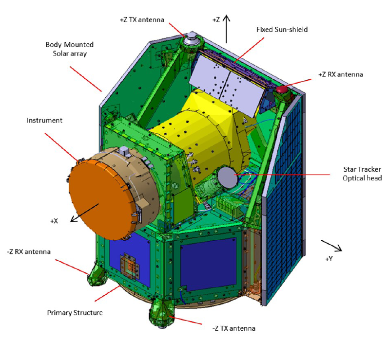
Figure 1: Adopted reference frame of the CHEOPS spacecraft. The $X$-axis coincides with the line of sight, while the $Z$-axis is antiparallel to the nadir direction. The $x$ and $y$ axes of the CCD coincide with the $-Y$ and $Z$ axes of the spacecraft, respectively. Image taken from Benz et al. (2020), courtesy of Airbus Defence and Space, Spain.

Table 3: Log of the CHEOPS observations of HD 108236. The last column gives the location of the target on the detector.

Planets	Start date	Duration	Valid points	File key	Efficiency	Exp. time	Location
	[UTC]	[h]	[#]		[%]	[s]	$(x;y)$ [px]
c, e	2020-03-10T18:09:15.9	18.33	983	CH_PR300046_TG000101_V0102	55	42	$(815;281)$
d	2020-04-28T07:06:11.0	18.63	770	CH_PR100031_TG015401_V0102	55	49	$(257;859)$
b, f	2020-04-30T17:06:11.0	17.04	674	CH_PR100031_TG015702_V0102	60	49	$(257;859)$

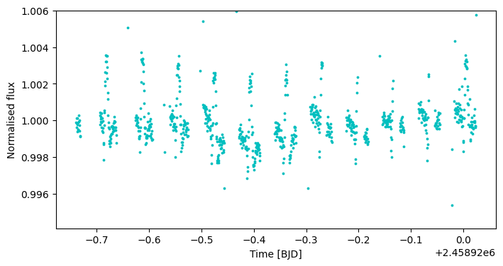
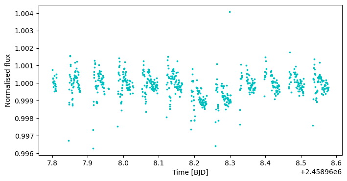
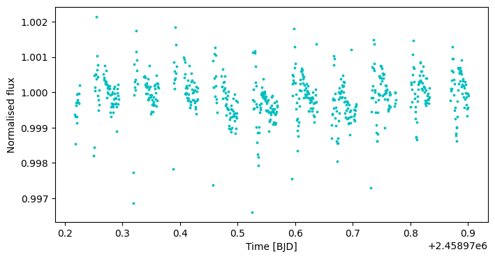
Figure 2: Raw LCs of the three CHEOPS visits analysed here, as processed by the Data Reduction Pipeline v12. The datasets are presented from top to bottom in chronological order of observation. The periodical light variations, especially visible in the first visit, correlate with the roll angle (see the text for further details).

Three observation runs, or visits, of HD 108236 were obtained with CHEOPS (Figure 2). The first visit, of 18.33 h duration, was obtained during the IOC phase using exposure times of 42 s. The other two visits, with a total duration 18.63 h and 17.04 h, were obtained during routine operations of the satellite using exposure times of 49 s. The observations were interrupted by Earth occultations and/or by South Atlantic Anomaly (SAA) crossings, where no data were downlinked, yielding an observing efficiency of 55%, 55%, and 60%, respectively, for each visit. The observing log of the CHEOPS data is presented in Table 3. We also note that the target location on the CCD has changed from March to April. This relocation of the target on the CCD has been done to avoid hot pixels. The project science office constantly monitors the hot pixels status on the detector and if keeping the pre-selected target location implies a significant loss in the expected performances, then the location is changed.

The raw data were automatically processed by the CHEOPS Data Reduction Pipeline (DRP v12; Hoyer et al., 2020). The DRP calibrates and corrects the images for instrumental and environmental effects, and finally performs aperture photometry of the target (Figure 3). As described in Hoyer et al. (2020), the DRP uses the Gaia catalogue (Gaia Collaboration et al., 2018) to simulate the FoV of the observations so to estimate the level of contamination in the photometric aperture. This is achieved by rotating background stars around the spacecraft $X$-axis and/or by the smear trails produced by bright stars in the CCD, in order to mimic the rotating CHEOPS FoV. In particular, in v12 of the DRP the smear contamination is automatically removed while the background stars’ contamination within the aperture (noticeably there is a 4.8 mag star $\sim$342 arcsec from HD 108236) is provided as a product to be used for further detrending during the data analysis. Finally, the DRP extracts the photometry using 3 fixed aperture sizes (radii of 22.5, 25 and 30 arcsec) and an extra aperture, the size of which depends on the level of contamination of the FoV. In this work we used the LCs obtained with the DEFAULT aperture of 25 arcsec, which results in the smallest root mean square (RMS) in the resulting LCs.

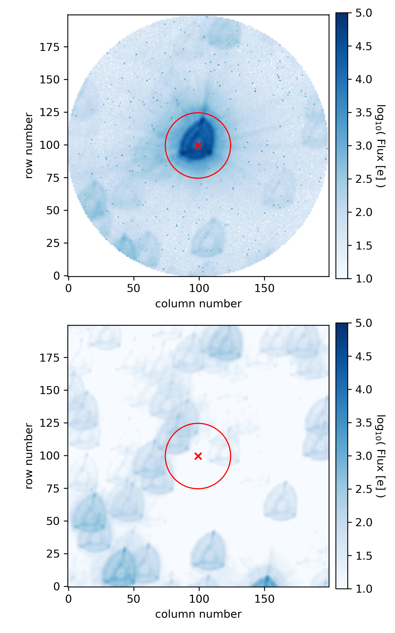
Figure 3: FoV of HD 108236. Top panel: Real FoV as observed by CHEOPS. Bottom panel: FoV as inferred from the DRP simulation with the target removed. The red cross indicates the location of the target’s PSF, while the photometric aperture is represented by the red circle. The horizontal (column number) and vertical (row number) axes correspond to the $x$ and $y$ axes of the CCD reference frame, respectively. Image scale is 1 arcsec per pixel.

We carefully inspected the LCs, looking for possible systematics. It turned out that the stellar flux presents particular patterns against the telescope roll angle in all three datasets, as shown in Figure 4. These flux variations against roll angle are likely due to an internal reflection from a very bright nearby star (HD 108257, $V\,=\,4.8$ mag), located 342 arcsec away (see Figure 5). This internal reflection produces a sort of slanted moving bar, which is visible in several frames, as shown in Figure 6.

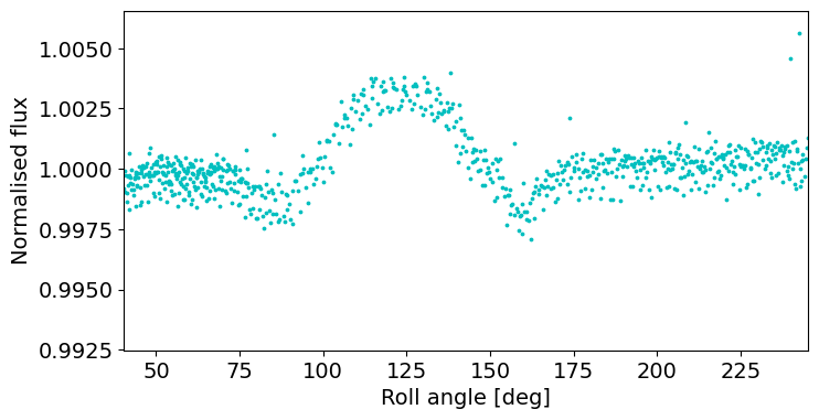
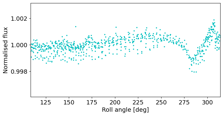
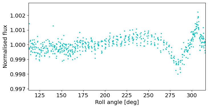
Figure 4: Dependence of flux against roll angle. The three CHEOPS datasets are presented from top to bottom in chronological order of observation.

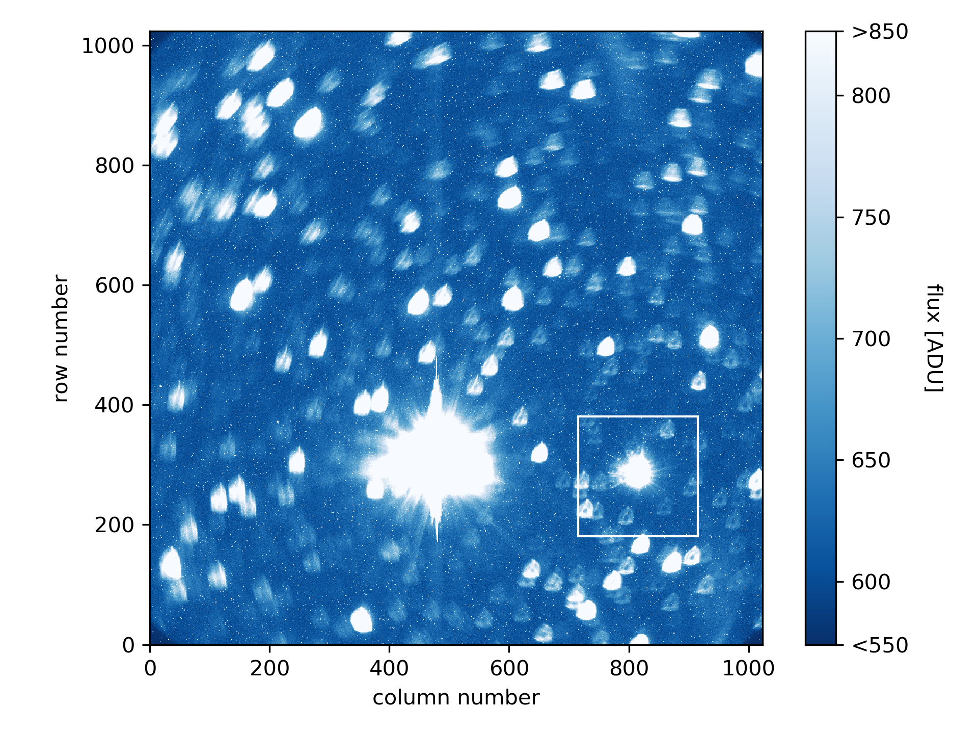
Figure 5: Full frame image of the first CHEOPS visit. The white square represents the location and size of the subarray window containing the target. The bright star located on the left of the white square is HD 108257, which probably produces the internal reflection generating the flux vs roll angle patterns shown in Fig. 4.

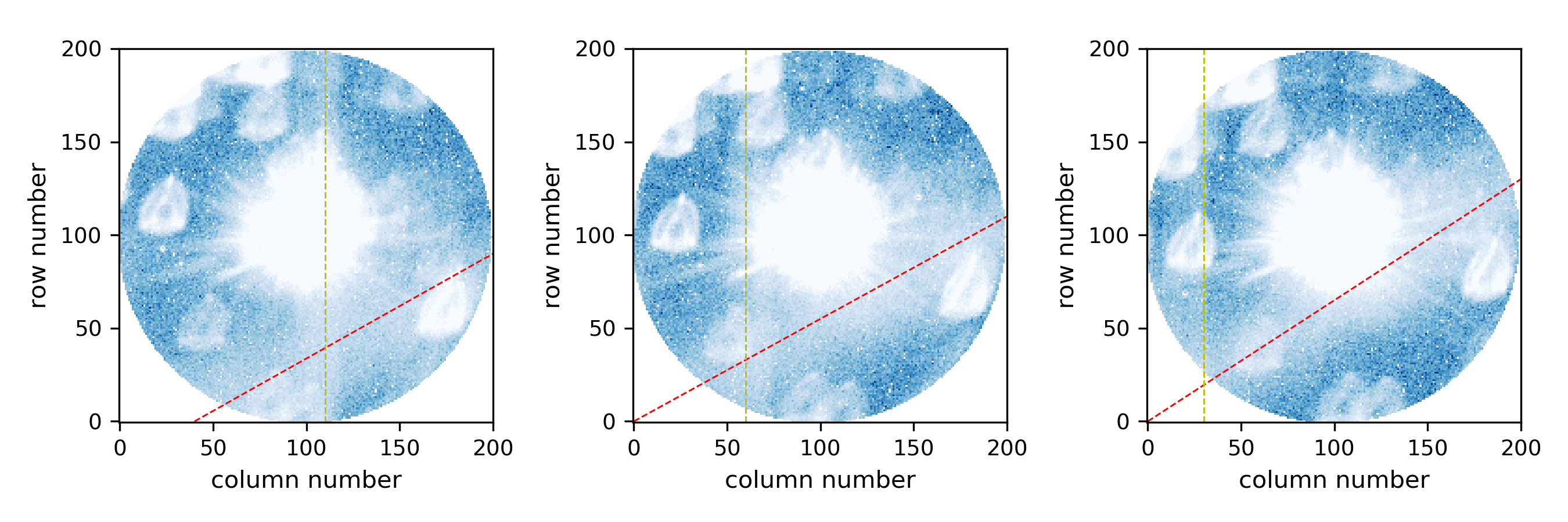
Figure 6: Set of frames taken from the first CHEOPS visit. The vertical dashed line indicates the smearing pattern, while the dashed red line indicates another pattern likely produced by the internal reflection of a contaminating source, which could be the nearby bright star HD 108257.

The specific pattern of flux versus roll angle produced by this contamination depends on the location of the target on the CCD. As reported in Table 3, the $(x;y)$ coordinates of the target in the first visit differ from those in the following two visits. In addition, the roll angle rotation rate is not constant with time, and it depends on the target’s coordinates with respect to the anti-Sun direction. By observing the same target at different epochs, the rotation rate of the spacecraft around the $X$-axis also changes, leading to variations in the rate at which the slanted bar moves. Consistently with this, the flux versus roll angle pattern shown in the top panel of Figure 4 (mid-March observations) differs from that shown in the middle and bottom panels, which are similar (both observations were taken at the end of April). With this in mind, we detrended the CHEOPS LCs versus roll angle (see Section 4).

3.2 TESS

In addition to the three CHEOPS datasets, we included the TESS data analysed by D20. HD 108236 was observed by TESS in sectors 10 (26 March 2019 - 22 April 2019) and 11 (22 April 2019 - 21 May 2019). Therefore, combining the TESS and CHEOPS data significantly increases the baseline, enabling us to improve the transit ephemerides and the system parameters (see Section 5.2). We analysed the TESS and CHEOPS data separately, to compare the performances, and together, to better constrain the system parameters.

We used the TESS data as processed by the Science Processing Operations Center (SPOC; Jenkins et al., 2016) pipeline. In particular, we considered the Pre-search Data Conditioned Simple Aperture Photometry (PDCSAP) flux values with their uncertainties as they are corrected for instrumental variations and represent the best estimate of the intrinsic flux variation of the target.

4 Data analysis

We carried out the LC analysis using allesfitter (Günther & Daylan, 2020). Among its features, this framework allows one to model exoplanetary transits using the ellc package (Maxted, 2016), further considering multi-planetary systems, TTVs, and Gaussian processes (GPs; Rasmussen & Williams, 2005) for the treatment of correlated noise, implemented through the celerite package (Foreman-Mackey et al., 2017). The parameters of interest are retrieved considering a Bayesian approach, which may use either the emcee package (Foreman-Mackey et al., 2013) implementing a MCMC method (see e.g. Ford, 2005) to sample the posterior probability distribution, or the Nested Sampling inference algorithm (see e.g. Feroz & Hobson, 2008; Feroz et al., 2019). In our work, we used the Dynamic Nested Sampling algorithm to have a direct estimate of the Bayesian evidence thanks to the dynesty package (Speagle, 2020).

Since allesfitter is not able to account for the flux dependence against roll angle seen in the CHEOPS data, we detrended the flux dependence versus roll angle through a Matérn-3/2 GP before inserting the CHEOPS LCs into allesfitter. The detrending was done using the celerite package, which gives the GP model and its variance. The GP model was computed using only the out-of-transit data points. Then, new enhanced error bars have been associated with the data points through error propagation accounting for the observational errors and the variance of the GP model.

Throughout the analysis, we assumed Gaussian priors on the following fitted parameters: the mean stellar density $\rho_{\star}=1.82\pm 0.12$ g/cm³, derived from our stellar characterisation, and the quadratic limb darkening (LD) coefficients $(q_{1},q_{2})$, inferred from the atlas9 models. In particular, we derived the $u_{1}$ and $u_{2}$ coefficients of the quadratic LD law using the code of Espinoza & Jordán (2015), that performs a cubic spline interpolation within the models according to the same procedure followed by Claret & Bloemen (2011). After that, we converted $u_{1}$ and $u_{2}$ to the quadratic LD coefficients $q_{1}$ and $q_{2}$ required by allesfitter following the relations of Kipping (2013), obtaining $(q_{1},q_{2})=(0.34,0.27)$ for the TESS bandpass, and $(q_{1},q_{2})=(0.46,0.32)$ for the CHEOPS bandpass. A 1-$\sigma$ uncertainty of 0.05 was attributed to all LD coefficients. We verified that this uncertainty value is conservatively in agreement with the priors estimated by Maxted (2018), who discussed the application of the power-2 LD law to the LCs of transiting exoplanets.

For each planet, the fitted parameters were: the ratio of planetary radius over stellar radius $R_{p}$/$R_{\star}$, the sum of stellar and planetary radius scaled to the orbital semi-major axis $(R_{p}+R_{\star})$/$a$, the cosine of the orbital inclination $\cos{i_{p}}$, the transit timing $T_{0}$, the orbital period $P$, and $\sqrt{e}\cos{\omega}$ and $\sqrt{e}\sin{\omega}$, where $e$ is the orbital eccentricity and $\omega$ is the argument of pericentre. The initial priors used in our fits are listed in Table 11.

The CHEOPS LCs, both binned and unbinned, with superimposed best-fit transit models, are shown in Figures 7, 8, and 9. In each Figure presenting TESS or CHEOPS LCs, the binned data are shown by combining 12 data points, independently of the exposure times. In the case of the CHEOPS LCs, each rebinned data point corresponds to 8.4 min in the case of the first visit and 9.8 min in the case of the last two visits.

During the inspection of the CHEOPS dataset with file key CH_PR100031_TG015702_V0102 (i.e. last observation), besides finding the expected transit of HD 108236 b at $T_{0,\mathrm{b,CH}}\sim$2458970.7 BJD, we serendipitously detected a transit-like feature (depth $\sim$400 ppm) occurring $\sim$0.2 days earlier than $T_{0,\mathrm{b,CH}}$ (i.e. $T_{0,\mathrm{f,CH}}\sim$2458970.5 BJD, see Figure 9). From this moment on, we will refer to this planet as HD 108236 f.

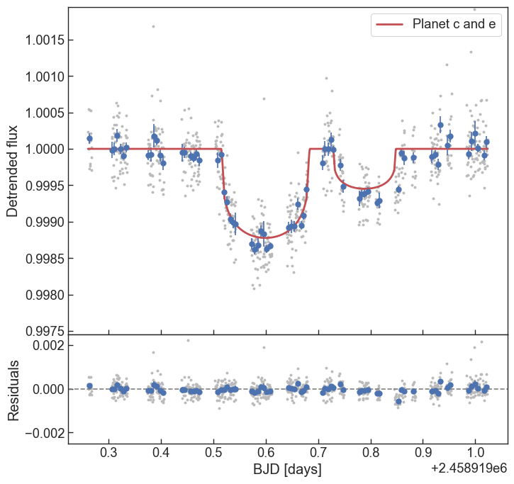
Figure 7: Detrended CHEOPS LC (first visit, file key CH_PR300046_TG000101_V0102) containing the transits of HD 108236 c at $T_{0,\mathrm{c,CH}}\sim$2458919.8 BJD and HD 108236 e at $T_{0,\mathrm{e,CH}}\sim$2458919.6 BJD. The red line shows the best-fit transit model, while the bottom panel shows the residuals following removal of the transit model.

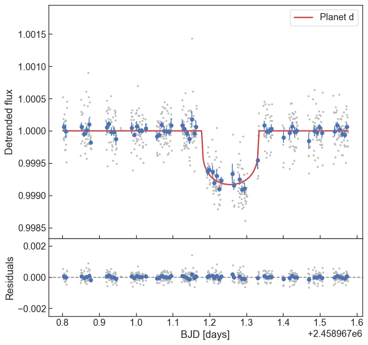
Figure 8: Same as Figure 7, but for HD 108236 d (second visit, file key CH_PR100031_TG015401_V0102).

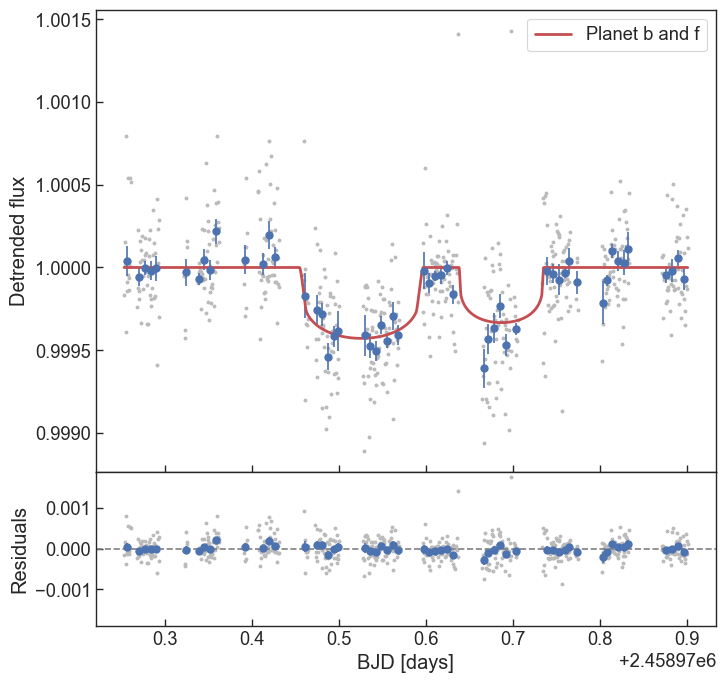
Figure 9: Same as Figure 7, but for HD 108236 b and HD 108236 f (third visit, file key CH_PR100031_TG015702_V0102). The transit of HD 108236 b is that at $T_{0,\mathrm{b,CH}}\sim$2458970.7 BJD, while the unexpected transit of HD 108236 f is that at $T_{0,\mathrm{f,CH}}\sim$2458970.5 BJD.

Bearing in mind this new detection, we decided to carry out analyses of the available datasets both considering four-planet and five-planet fitting scenarios. To establish whether one model ($\mathcal{M}_{1}$) is to be preferred over the other ($\mathcal{M}_{0}$), we computed the Bayes factor $\mathcal{B}_{10}$, which is defined as (Kass & Raftery, 1995):

$$\mathcal{B}_{10}=\frac{\mathcal{Z}_{1}}{\mathcal{Z}_{0}}\,,$$ (6)

where $\mathcal{Z}_{i}$ is the Bayesian evidence (i.e. the marginal likelihood integrated over the entire parameter space) referring to the $i$-th model. The value of $\mathcal{Z}$ is given by the Nested Sampling algorithm, thus $\mathcal{B}_{10}$ could be straightforwardly computed through Equation (6). The higher the $\mathcal{B}_{10}$, the higher the evidence against $\mathcal{M}_{0}$ ( i.e. $\mathcal{M}_{1}$ is to be preferred). Reference values of $\mathcal{B}_{10}$ and corresponding levels of evidence against $\mathcal{M}_{0}$ are reported in Kass & Raftery (§3.2; 1995). Here we just recall that very strong evidence against the null hypothesis $\mathcal{M}_{0}$ (i.e. $\mathcal{M}_{1}$ is strongly favoured) occurs when $\ln{\mathcal{B}_{10}}>5$.

5 Results and discussion

5.1 Additional planets in the system

The detected transit-like signal visible in Figure 9 at $T_{0,\mathrm{f,CH}}\sim$2458970.5 BJD does not show any correlation with the flux of field stars that contaminate the aperture photometry (estimated as explained in Hoyer et al., 2020), nor with background light, nor with aperture size. In addition, the temporal stability of the $(x;y)$ coordinates of the PSF centroid suggests the absence of any PSF jumps, hence no new hot pixels have appeared inside the PSF area during the observation (see Figure 10). Furthermore, by analysing the raw data, the DRP team confirmed that this feature cannot be ascribed to telegraphic pixels (i.e. pixels that occasionally blink and twinkle), nor to cosmic rays or any spacecraft instrumental metrics.

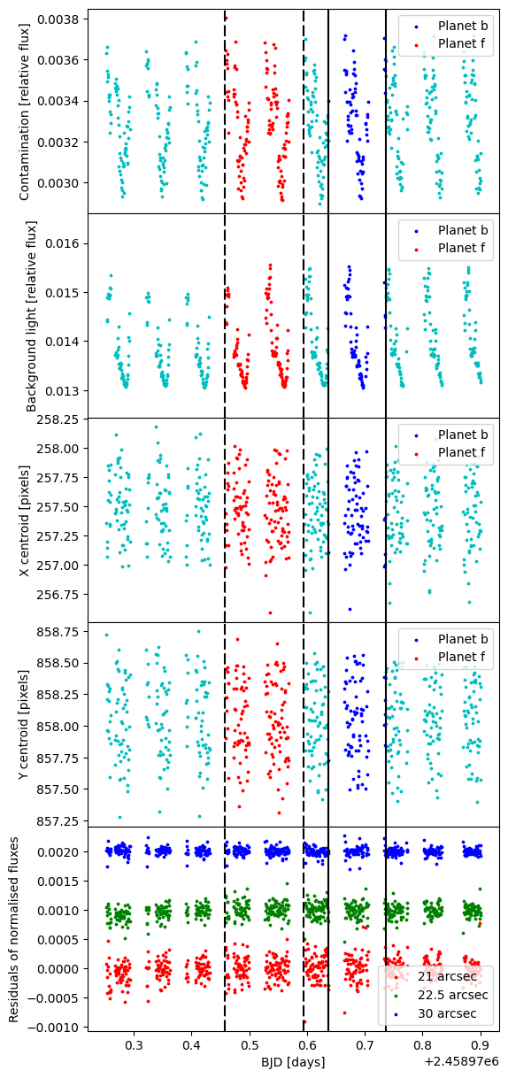
Figure 10: All the represented quantities expressed as a function of time during the third CHEOPS visit (i.e. the one containing the transits of HD 108236 b and HD 108236 f). Top two panels: flux of contaminating stars entering the photometric aperture and background light (both relative to the flux of HD 108236). Third and fourth panels from top: $x$- and $y$-coordinate of the PSF centroid. The transit windows of planets b and f are highlighted in blue and red, respectively, while the out-of-transit points are in cyan. Bottom panel: residuals of the normalised fluxes (shifted vertically for visualisation purposes) obtained after subtracting the reference normalised flux computed considering the DEFAULT aperture to the normalised fluxes computed considering the other three available apertures. No correlation is present between flux and aperture size. Transit windows of planets b and f are marked by solid and dashed vertical lines, respectively.

Therefore, given the transit-like nature of the signal, we looked for similar features, in terms of both transit depth and duration, in the available TESS LCs. Indeed, we spotted a similar signal in the second TESS LC (sector 11) at $T_{0\mathrm{,f,TE11}}$ $\sim$ 2458616.04 BJD by visual inspection (Figure 11). We applied both a four-planet and five-planet fit to these TESS data and compared the RMS of the residuals binned on a 24 min timescale within the [2458615.9, 2458616.2] BJD window, which contains the supposed transit. We obtained RMS values of 130 ppm and 154 ppm for the five-planet and four-planet scenarios, respectively. The lowest RMS value in the five-planet case shows how the transit model may justify the flux variability; as a term of comparison the RMS of the binned residuals over the entire sector 11 is 152 ppm.

Then, we carefully inspected the TESS sector 10 LC as well, looking for further undetected signals compatible with a d$F$ $\sim$ 400 ppm. We noticed that $\sim$ 29.5 days before the supposed transit of HD 108236 f, HD 108236 e is transiting, but the assumption of four planets keeps some additional flux variability when the transit model is subtracted from the data points (see Figure 12). We wondered whether the structures seen in the signal could be ascribed to a further undetected transit, that is whether the layout of the data points could be justified by a double transit. By including the transit model of HD 108236 f, we significantly improve the quality of the fit as shown in Figure 13. Considering the temporal window [2458586.4, 2458586.7] BJD, the RMS of the binned residuals on a 24 minutes timescale is 137 ppm for the five-planet scenario versus 168 ppm for the four-planet scenario. As a term of comparison, the RMS of the binned residuals over the entire sector 10 LC is 158 ppm. The presence of HD 108236 f also affects the transit depth of HD 108236 e, d$F_{\mathrm{e}}$. From the five-planet scenario we inferred d$F_{\mathrm{e}}=1038_{-28}^{+30}$ ppm, while the four-planet scenario yields to a deeper transit with d$F_{\mathrm{e}}=1056_{-36}^{+37}$ ppm, as expected.

The temporal difference between these two transits of HD 108236 f in the two TESS sectors gives a candidate value for the orbital period, which also agrees with the transit epoch of the signal detected in the CHEOPS visit. Therefore, we propose $P=29.54$ days as a possible candidate value.

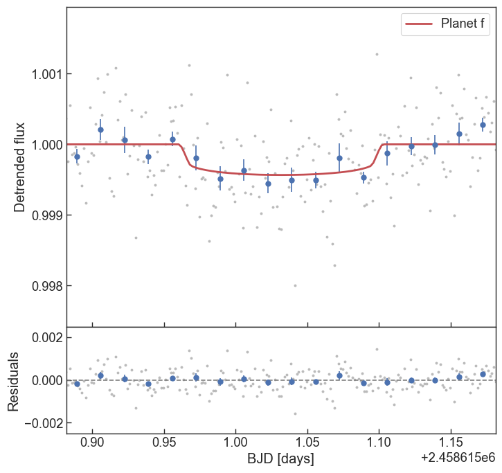
Figure 11: Portion of the TESS sector 11 LC. Data are binned on a timescale of 24 min. The red solid line shows the transit model for HD 108236 f. Neglecting the presence of HD 108236 f and performing a four-planet fit, the RMS of the binned residuals would be 154 ppm. Instead, a five-planet fit reduces the RMS of the binned residuals to 130 ppm.

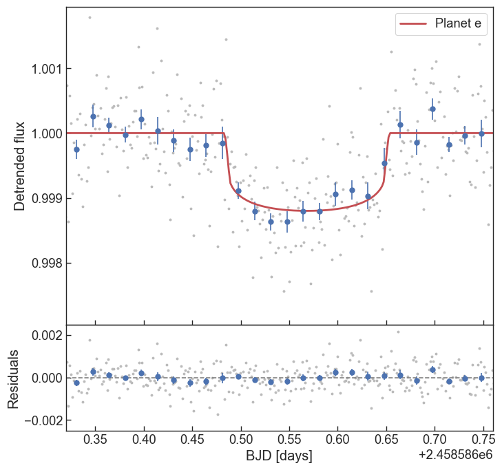
Figure 12: Portion of the TESS sector 10 LC. The solid red line represents the model of the transit of HD 108236 e considering the four-planets scenario: a residual variability in the data points remains unexplained. Data are binned on a timescale of 24 min; the RMS of the binned residuals over the transit window is 168 ppm.

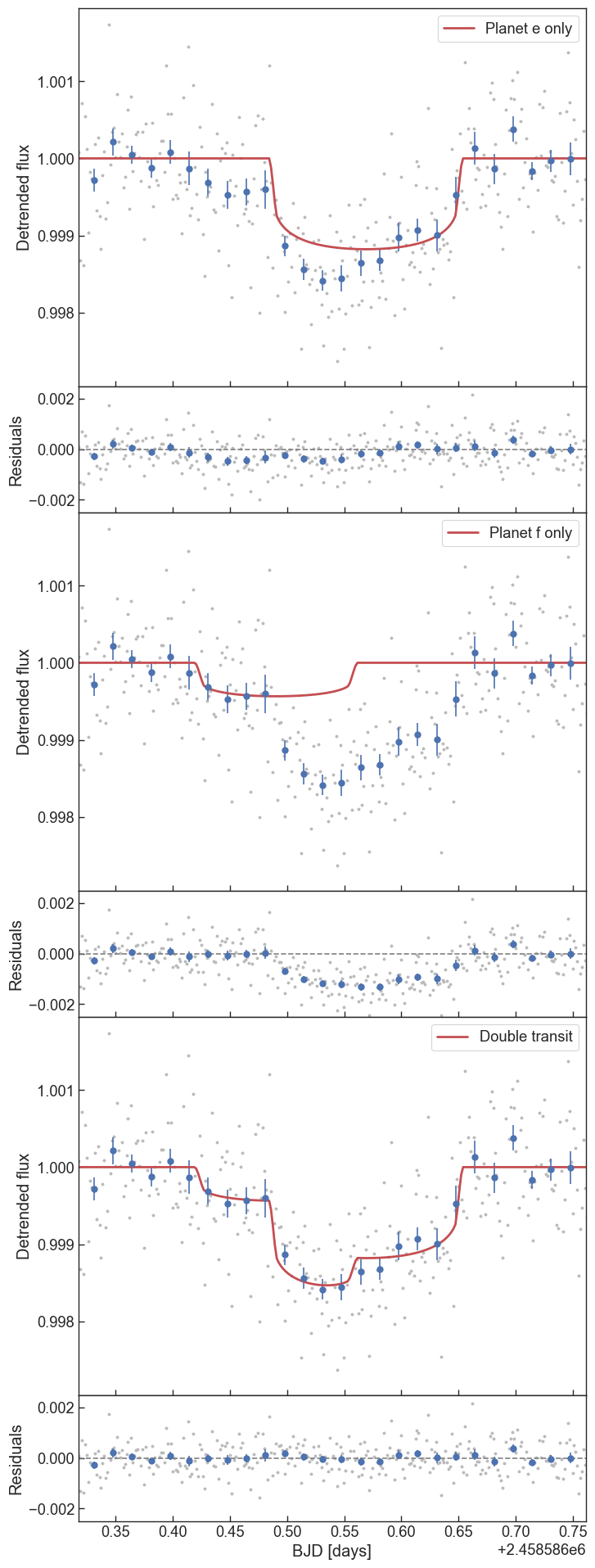
Figure 13: Same as Figure 12, but considering the five-planet fit. The top and middle panels show the transits of HD 108236 e and HD 108236 f separately, while the bottom panel shows the results obtained with the combined model. The RMS of the binned residuals over the transit window is 137 ppm, which is lower than 168 ppm retrieved in the four-planet scenario, where HD 108236 f is absent.

D20 investigated whether additional planets may be present in the system and proposed a possible candidate with a period of 10.9113 days, with $T_{0}=2458570.6781$ BJD and a transit depth of 230 ppm. However, they cautioned that this is only a candidate because the false alarm probability of 0.01 is influenced by the detrending method and the detected features might be instrumental in origin. As the TESS dataset cannot give a definitive answer, we looked for possible signals of this candidate in the CHEOPS LCs. Propagating its ephemeris, we would expect a transit of this candidate planet at $T_{0}=2458919.839$ BJD, hence blended with the transit of HD 108236 c. We ran a further analysis of the CHEOPS LC, covering the transit of HD 108236 c considering a scenario with six planets and compared the results with the favoured scenario with five planets (null hypothesis), obtaining $\ln{\mathcal{B}_{65}}=-10.6\Rightarrow\ln{\mathcal{B}_{56}}=10.6>5$, which means that there is a strong evidence for not rejecting the null hypothesis. On the one hand, the Bayes factor strongly disfavours the presence of a planet at $\sim$10.9 days. On the other hand, the putative transit would be shallow and blended with the transit of HD 108236 c. Therefore, further LCs are needed to give a definitive answer.

5.2 Comparative photometric analysis

We carried out the analysis considering the TESS and CHEOPS datasets separately (’TESS-only’ and ’CHEOPS-only’ approaches) and combined (’TESS+CHEOPS’ approach). As the CHEOPS-only approach involved the analysis of one single transit per planet, we imposed a normal prior on the orbital periods based on the results obtained from the TESS-only approach. For each approach, we fitted the data considering both four and five planets. The four-planet fit considered the four planets from HD 108236 b to HD 108236 e already detected by D20, while the five-planet fit also included the planet HD 108236 f with an orbital period of $\sim$ 29.5 days. Here we recall that, according to our discussion in Section 5.1, there should be just two transits of HD 108236 f in the whole TESS dataset, and one is blended with a transit of HD 108236 e.

The Bayesian factors $\mathcal{B}_{54}$ obtained from the different approaches, where we tested the five-planet scenario against the four-planet scenario, are reported in Table 4. The $\ln{\mathcal{B}_{54}}$ Bayesian indicator (which is always greater than 5) strongly favours the scenario with five transiting planets.

Table 4: Natural logarithm of the Bayes factors obtained when testing the five-planet scenario against the four-planet scenario for each of our three approaches.

	TESS-only	CHEOPS-only	TESS+CHEOPS
$\ln{\mathcal{B}_{54}}$	10.8	13.4	13.1

Supported by the Bayesian evidence, we consider the five-planet scenario to be the most appropriate description of the data. Table 5 summarises the results obtained for this scenario. At first, we performed all analyses considering the orbital eccentricity $e$ as a free parameter, as also done by D20. Then, we analysed the dynamical stability of our TESS+CHEOPS solution (see Section 5.3 for further details), finding that the lack of a constraint on $e$ leads to a severely unstable system. Therefore, we repeated the TESS+CHEOPS analysis setting $e\lesssim 0.1$, which is also supported by the dynamical stability analysis of D20 (see their Figure 16). The last column of Table 5 presents our reference results, accounting for the constraint on $e$ and considering all available datasets. We emphasise that in Table 5 all reported transit depths are intended to be $\mathrm{d}F\equiv\left(\frac{R_{p}}{R_{\star}}\right)^{2}$ to make them comparable between CHEOPS and TESS, that is to say independent of the instrumental bandpass and thus specific limb darkening.

Table 5: HD 108236 system parameters obtained from analyses of the TESS and CHEOPS LCs, in comparison to what was found by Daylan et al. (2020). The columns labelled as TESS-only, CHEOPS-only, and TESS+CHEOPS refer to the results obtained considering five transiting planets in the system. All results have been obtained considering $e$ as a free parameter, except for the last column for which $e$ has been set to be smaller than 0.1. The TESS+CHEOPS analysis with $e<0.1$ gives our final adopted solution for the system.

Parameters			Daylan et al. (2020)	TESS-only	CHEOPS-only	TESS+CHEOPS
			$e$ free	$e$ free	$e$ free	$e$ free	$e<0.1$
Planet b: 12 TESS transits; 1 CHEOPS transit
Eclipse timing	$T_{0}$	[BJD]	$8572.1128_{-0.0036}^{+0.0031}$	$8598.6796_{-0.0025}^{+0.0019}$	$8947.9067_{-0.0020}^{+0.0055}$	$8773.2959_{-0.0017}^{+0.0012}$	$8773.2964\pm 0.0013$
Period	$P$	[days]	$3.79523_{-0.00044}^{+0.00047}$	$3.79517_{-0.00037}^{+0.00040}$	$3.79527_{-0.00013}^{+0.00013}$	$3.795954_{-0.000034}^{+0.000029}$	$3.795963_{-0.000034}^{+0.000025}$
Transit depth	d$F$	[ppm]	$268\pm 31$	$267_{-24}^{+26}$	$337_{-45}^{+36}$	$273\pm 17$	$285\pm 17$
Transit duration	$W$	[h]	$2.30_{-0.11}^{+0.16}$	$2.35_{-0.28}^{+0.17}$	$2.09_{-0.29}^{+0.35}$	$2.46_{-0.15}^{+0.12}$	$2.384\pm 0.093$
Impact parameter	$b$	[$R_{\star}$]	$0.38\pm 0.24$	$0.48_{-0.15}^{+0.17}$	$0.65_{-0.19}^{+0.11}$	$0.43\pm 0.12$	$0.452_{-0.096}^{+0.071}$
Semi-major axis	$a$	[AU]	$0.0469\pm 0.0017$	$0.04505\pm 0.00077$	$0.04454_{-0.0012}^{+0.00083}$	$0.04436\pm 0.00081$	$0.04527_{-0.00088}^{+0.00096}$
Orbital inclination	$i_{p}$	[∘]	$87.88_{-0.87}^{+1.30}$	$87.47_{-0.59}^{+0.65}$	$86.04_{-0.44}^{+0.50}$	$87.51_{-0.50}^{+0.58}$	$87.59_{-0.35}^{+0.47}$
Eccentricity	$e$		$0.20_{-0.14}^{+0.30}$	$0.130_{-0.094}^{+0.18}$	$0.22_{-0.17}^{+0.19}$	$0.20_{-0.11}^{+0.15}$	$0.045_{-0.033}^{+0.039}$
Arg. of pericentre	$\omega$	[∘]	$190\pm 140$	$262_{-230}^{+77}$	$49_{-32}^{+130}$	$166_{-30.}^{+21}$	$126_{-62}^{+51}$
Radius	$R_{p}$	[$R_{\oplus}$]	$1.586\pm 0.098$	$1.563_{-0.072}^{+0.078}$	$1.756_{-0.12}^{+0.096}$	$1.579\pm 0.052$	$1.615\pm 0.051$
Planet c: 8 TESS transits; 1 CHEOPS transit
Eclipse timing	$T_{0}$	[BJD]	$8572.3949_{-0.0020}^{+0.0025}$	$8597.2096_{-0.0015}^{+0.0015}$	$8944.6086_{-0.0021}^{+0.0022}$	$8770.90623_{-0.00071}^{+0.00071}$	$8770.90586_{-0.00078}^{+0.00078}$
Period	$P$	[days]	$6.20370_{-0.00052}^{+0.00064}$	$6.20381_{-0.00043}^{+0.00037}$	$6.20380_{-0.00012}^{+0.00013}$	$6.203468_{-0.000049}^{+0.000035}$	$6.203449_{-0.000046}^{+0.000049}$
Transit depth	d$F$	[ppm]	$455_{-35}^{+40}$	$429_{-23}^{+27}$	$524_{-25}^{+32}$	$483_{-20}^{+21}$	$469_{-22}^{+21}$
Transit duration	$W$	[h]	$2.913\pm 0.095$	$2.948_{-0.13}^{+0.099}$	$2.81_{-0.19}^{+0.14}$	$2.915\pm 0.10$	$2.86_{-0.11}^{+0.10}$
Impact parameter	$b$	[$R_{\star}$]	$0.33_{-0.21}^{+0.25}$	$0.30\pm 0.12$	$0.43_{-0.13}^{+0.12}$	$0.441_{-0.079}^{+0.063}$	$0.455_{-0.083}^{+0.069}$
Semi-major axis	$a$	[AU]	$0.0651\pm 0.0024$	$0.0638_{-0.0011}^{+0.0011}$	$0.06372_{-0.00082}^{+0.00086}$	$0.0612\pm 0.0010$	$0.0620\pm 0.0012$
Orbital inclination	$i_{p}$	[∘]	$88.72_{-0.74}^{+0.82}$	$88.87\pm 0.42$	$88.29_{-0.41}^{+0.47}$	$88.28_{-0.22}^{+0.27}$	$88.30_{-0.23}^{+0.29}$
Eccentricity	$e$		$0.18_{-0.14}^{+0.34}$	$0.069_{-0.050}^{+0.099}$	$0.098_{-0.063}^{+0.081}$	$0.054_{-0.038}^{+0.073}$	$0.034_{-0.025}^{+0.042}$
Arg. of pericentre	$\omega$	[∘]	$210\pm 120$	$164_{-100.}^{+120}$	$89\pm 53$	$97_{-75}^{+230}$	$211_{-110}^{+44}$
Radius	$R_{p}$	[$R_{\oplus}$]	$2.068_{-0.091}^{+0.100}$	$1.981_{-0.058}^{+0.064}$	$2.190_{-0.056}^{+0.071}$	$2.102\pm 0.050$	$2.071\pm 0.052$
Planet d: 4 TESS transits; 1 CHEOPS transit
Eclipse timing	$T_{0}$	[BJD]	$8571.3368_{-0.0013}^{+0.0015}$	$8599.68768_{-0.00095}^{+0.0013}$	$8954.0698_{-0.0030}^{+0.0096}$	$8769.79772_{-0.00083}^{+0.0014}$	$8769.79682_{-0.00090}^{+0.00090}$
Period	$P$	[days]	$14.17555_{-0.00110}^{+0.00099}$	$14.1756\pm 0.0011$	$14.17549_{-0.00048}^{+0.00053}$	$14.175748_{-0.000067}^{+0.00010}$	$14.175685_{-0.00010}^{+0.000083}$
Transit depth	d$F$	[ppm]	$787\pm 53$	$740_{-33}^{+38}$	$788_{-58}^{+59}$	$754\pm 29$	$705_{-34}^{+31}$
Transit duration	$W$	[h]	$3.734_{-0.049}^{+0.066}$	$4.022_{-0.26}^{+0.088}$	$2.71_{-0.32}^{+1.3}$	$3.954_{-0.11}^{+0.097}$	$3.85_{-0.13}^{+0.18}$
Impact parameter	$b$	[$R_{\star}$]	$0.35_{-0.21}^{+0.19}$	$0.25_{-0.14}^{+0.19}$	$0.776_{-0.61}^{+0.067}$	$0.327\pm 0.075$	$0.423_{-0.13}^{+0.070}$
Semi-major axis	$a$	[AU]	$0.1131\pm 0.0040$	$0.1093_{-0.0022}^{+0.0019}$	$0.1100_{-0.0018}^{+0.0021}$	$0.1087\pm 0.0020$	$0.1074\pm 0.0023$
Orbital inclination	$i_{p}$	[∘]	$89.22_{-0.38}^{+0.45}$	$89.40_{-0.37}^{+0.33}$	$88.462_{-0.081}^{+0.43}$	$89.25_{-0.15}^{+0.16}$	$89.06_{-0.14}^{+0.27}$
Eccentricity	$e$		$0.17_{-0.12}^{+0.30}$	$0.17_{-0.11}^{+0.18}$	$0.24_{-0.17}^{+0.51}$	$0.071_{-0.036}^{+0.038}$	$0.055_{-0.035}^{+0.038}$
Arg. of pericentre	$\omega$	[∘]	$190_{-130}^{+140}$	$167_{-70.}^{+24}$	$224_{-67}^{+61}$	$79_{-41}^{+46}$	$151_{-33}^{+46}$
Radius	$R_{p}$	[$R_{\oplus}$]	$2.72\pm 0.11$	$2.603_{-0.065}^{+0.072}$	$2.684_{-0.099}^{+0.10}$	$2.626\pm 0.057$	$2.539_{-0.065}^{+0.062}$
Planet e: 2 TESS transits; 1 CHEOPS transit
Eclipse timing	$T_{0}$	[BJD]	$8586.5677_{-0.0014}^{+0.0014}$	$8606.1591_{-0.0010}^{+0.0014}$	$8939.1926_{-0.0018}^{+0.0037}$	$8782.46937_{-0.00062}^{+0.00067}$	$8782.46935_{-0.00069}^{+0.00078}$
Period	$P$	[days]	$19.5917^{+0.0022}_{-0.0020}$	$19.5899\pm 0.0018$	$19.59087_{-0.00047}^{+0.00053}$	$19.589970_{-0.000074}^{+0.000074}$	$19.590025_{-0.000089}^{+0.000083}$
Transit depth	d$F$	[ppm]	$1043^{+78}_{-71}$	$1003_{-50}^{+55}$	$1049_{-47}^{+39}$	$1036_{-25}^{+31}$	$1038_{-28}^{+30}$
Transit duration	$W$	[h]	$4.013^{+0.080}_{-0.057}$	$4.12_{-0.30}^{+0.26}$	$4.22_{-0.18}^{+0.20}$	$4.38_{-0.19}^{+0.15}$	$4.20_{-0.13}^{+0.13}$
Impact parameter	$b$	[$R_{\star}$]	$0.36^{+0.20}_{-0.23}$	$0.47_{-0.15}^{+0.12}$	$0.464_{-0.11}^{+0.080}$	$0.374\pm 0.10$	$0.426_{-0.077}^{+0.059}$
Semi-major axis	$a$	[AU]	$0.1400\pm 0.0052$	$0.1362\pm 0.0026$	$0.1333\pm 0.0017$	$0.1341\pm 0.0020$	$0.1367_{-0.0020}^{+0.0022}$
Orbital inclination	$i_{p}$	[∘]	$89.32^{+0.42}_{-0.30}$	$89.09_{-0.20}^{+0.19}$	$89.14_{-0.11}^{+0.17}$	$89.28_{-0.14}^{+0.18}$	$89.245_{-0.086}^{+0.12}$
Eccentricity	$e$		$0.20^{+0.30}_{-0.13}$	$0.29_{-0.20}^{+0.41}$	$0.20_{-0.15}^{+0.27}$	$0.119_{-0.060}^{+0.086}$	$0.058_{-0.036}^{+0.032}$
Arg. of pericentre	$\omega$	[∘]	$170_{-130}^{+150}$	$194_{-44}^{+16}$	$192_{-21}^{+13}$	$136_{-42}^{+28}$	$128_{-54}^{+37}$
Radius	$R_{p}$	[$R_{\oplus}$]	$3.12^{+0.13}_{-0.12}$	$3.029_{-0.081}^{+0.088}$	$3.096_{-0.070}^{+0.066}$	$3.080_{-0.048}^{+0.054}$	$3.083\pm 0.052$
Planet f: 2 TESS transits; 1 CHEOPS transit
Eclipse timing	$T_{0}$	[BJD]		$8616.0418_{-0.0078}^{+0.0072}$	$8970.5257_{-0.0038}^{+0.0023}$	$8793.2785_{-0.0022}^{+0.0028}$	$8793.2786_{-0.0019}^{+0.0021}$
Period	$P$	[days]		$29.5461_{-0.0096}^{+0.0089}$	$29.54255_{-0.00069}^{+0.00069}$	$29.54075_{-0.00045}^{+0.00037}$	$29.54115_{-0.00042}^{+0.00033}$
Transit depth	d$F$	[ppm]		$366_{-59}^{+61}$	$416_{-18}^{+21}$	$474_{-32}^{+28}$	$445_{-24}^{+21}$
Transit duration	$W$	[h]		$4.90_{-1.1}^{+0.33}$	$4.05_{-0.33}^{+0.35}$	$3.39_{-0.28}^{+0.36}$	$3.27_{-0.15}^{+0.13}$
Impact parameter	$b$	[$R_{\star}$]		$0.38_{-0.22}^{+0.33}$	$0.665_{-0.082}^{+0.067}$	$0.793_{-0.061}^{+0.041}$	$0.808\pm 0.022$
Semi-major axis	$a$	[AU]		$0.1773\pm 0.0036$	$0.1759\pm 0.0037$	$0.1750\pm 0.0041$	$0.1758_{-0.0038}^{+0.0041}$
Orbital inclination	$i_{p}$	[∘]		$89.27_{-0.26}^{+0.40}$	$88.873_{-0.096}^{+0.066}$	$88.910_{-0.078}^{+0.074}$	$88.963\pm 0.042$
Eccentricity	$e$			$0.38\pm 0.23$	$0.245\pm 0.092$	$0.17_{-0.12}^{+0.19}$	$0.051_{-0.034}^{+0.036}$
Arg. of pericentre	$\omega$	[∘]		$167_{-67}^{+38}$	$91\pm 29$	$230_{-210}^{+120}$	$275_{-63}^{+45}$
Radius	$R_{p}$	[$R_{\oplus}$]		$1.83\pm 0.16$	$1.951_{-0.049}^{+0.054}$	$2.082_{-0.073}^{+0.065}$	$2.017_{-0.057}^{+0.052}$

As a sanity check, we also carried out an independent joint analysis of the TESS and CHEOPS LCs with the code pyaneti (Barragán et al., 2019), which estimates the transit parameters using a Bayesian approach. We imposed uniform priors for all fitted parameters. We sampled for the mean stellar density $\rho_{\star}$ and recovered the scaled semi-major axis for each planet ($a/R_{\star}$) using Kepler’s third law (Winn, 2010). The joint modelling of the transit LCs of the five planets provides a mean stellar density of $\rho_{\star}$ = 2.11${}^{+0.18}_{-0.20}$ g cm^-3, which agrees with the density of 1.82 $\pm$ 0.11 g cm^-3 derived from the stellar mass and radius presented in Sect. 2. The transit parameter estimates are consistent well within $\sim$ 1$\sigma$ with those derived with allesfitter, supporting our results.

We further carried out an independent analysis of the CHEOPS IOC LC using the pycheops package (Maxted et al., in prep), which is being developed specifically for the analysis of CHEOPS data (see Lendl et al., 2020, for more details). From this additional analysis, we obtained values (see Table 6) fully compatible with allesfitter results, namely with differences lying below 1.2$\sigma$.

Table 6: Results obtained from the pycheops analysis of the CHEOPS IOC LC (first visit). Differences are computed with respect to the CHEOPS-only results listed in Table 5.

Parameter	pycheops	Difference[$\sigma$]
Planet c
d$F$ [ppm]	530${}^{+67}_{-58}$	0.19
$W$ [h]	2.88$\pm$0.40	0.50
$b$	0.57${}^{+0.13}_{-0.22}$	1.17
Planet e
d$F$ [ppm]	1011${}^{+53}_{-54}$	0.81
$W$ [h]	4.02${}^{+0.14}_{-0.15}$	1.11
$b$	0.46${}^{+0.09}_{-0.13}$	0.04

We comment here in detail on the results listed in Table 5. The first column lists the results obtained by D20, which may be directly compared to our TESS-only results, given that both analyses use the same dataset and employ the same analysis tool. However, D20 employed an MCMC technique implemented through the emcee package, considered the presence of four transiting planets, and adopted $\rho_{\star,D20}=1.94\pm 0.16$ g/cm³ as prior. Instead, we employed the Dynamic Nested Sample technique implemented through the dynesty package, considered five transiting planets, and imposed a sharper Gaussian prior on the stellar density of $\rho_{\star}=1.82\pm 0.12$ g/cm³. Furthermore, we assumed normal Gaussian priors on the LD coefficients (see Section 4), while D20 set uniform priors on the LD coefficients. Despite the differences, all the TESS-only results are consistent within $\sim$1$\sigma$, but our results have in general smaller uncertainties, most likely because of the tighter priors on the stellar density and LD coefficients.

The comparison of the results obtained considering TESS and CHEOPS separately is important in order to assess the photometric precision of CHEOPS in comparison to that of TESS. The relative uncertainties $\delta$ on the transit depth $\mathrm{d}F$ are reported in Table 7. The values of $\delta$ are a function of the telescope effective diameter, the number of observed transits, the exposure time, and the transit depth. As a matter of fact, on the one hand, $b$, $e$, and $\omega$ are rather poorly constrained in the CHEOPS LCs due to the availability of single transits with frequent gaps and this affects our capability of reconstructing the transit model, especially in case of shallow transits. On the other hand, CHEOPS guarantees a greater (relative to TESS) photometric precision for shallower transits than for deeper transit as CHEOPS observations break through the TESS photometric noise floor (which limits the photometric precision of TESS for shallow transit). In the case of HD 108236, one CHEOPS transit observation leads to approximately the same level of precision in $\delta$ as eight TESS transits for $\mathrm{d}F\sim$500 ppm, which corresponds to the detection of a mini-Neptune with $R_{p}\sim$2  $R_{\oplus}$ around a solar-like star. For deeper transit signals ($\sim$1000 ppm), one CHEOPS transit observation leads to a precision on the transit depth higher than that of two TESS transits, roughly by a factor of 1.3. Finally, for shallower transits ($\sim$250 ppm), one CHEOPS transit observation leads to about the same precision on the transit depth obtained after about seven TESS transit observations. However, these conclusions depend on the length and location of gaps in the CHEOPS LCs.

Table 7: Comparison of the photometric precision reached by TESS (TE) and CHEOPS (CH), quantified by the relative uncertainty $\delta$ of the squared ratio between the planetary and stellar radius $\mathrm{d}F$. Results are also influenced by specific LC features, such as gaps, especially if they occur during the ingress or egress phases. Columns labelled with gap_ij express the temporal percentage of gaps occurring between the $i^{\mathrm{th}}$ and the $j^{\mathrm{th}}$ contact in CHEOPS LCs.

Planet	# Transits	$\mathrm{d}F$	gap12	gap23	gap34	Photometric error: $\delta$    [%]
	TE:CH	[ppm]	[%]	[%]	[%]	TESS-only	CHEOPS-only
b	12:1	250	47	67	0	9.3	12
c	8:1	500	0	38	100	5.8	5.4
d	4:1	750	100	54	56	4.8	7.4
e	2:1	1000	94	61	0	5.2	4.1
f	2:1	450	16	43	100	16	4.8

The comparison between the TESS+CHEOPS approach and the analyses performed considering TESS and CHEOPS LCs separately is not straightforward. One may generally expect that the results coming from the combined analysis fall somewhere in the middle of the range defined by the results of the separate analyses, but this is not always the case. The main reason is that the CHEOPS-only analysis is not always as robust as the TESS-only analysis. In fact, in the former we consider just one transit per planet, with the photometric signal of CHEOPS LCs that is affected by frequent gaps. In particular, we are missing the ingress and/or egress phase of each transit partially or totally (see Table 7). These are the most delicate phases of the transit as they best constrain the impact parameter $b$ and hence the orbital inclination $i_{p}$. The loose constraint on $b$ (due to the gaps in the LCs) and the treatment of $e$ and $\omega$ as free parameters (despite only photometric data are available) increase the degrees of freedom and hence the degeneracies within the multi-parametric transit model. This justifies the discrepancies among a few parameter values, like $\mathrm{d}F$ and $i_{p}$ of HD 108236 b or $i_{p}$ of HD 108236 d, involving the CHEOPS-only approach.

It is in the combined analysis where we can account for the numerous transits from TESS (which give much more indications about the transit shape, decreasing the degrees of freedom of the fitted model) and, simultaneously, on the exquisite CHEOPS photometry (which allows the refinement of all the fitted parameters as the robustness of the transit shape is guaranteed by TESS). In particular, Table 8 shows the relative uncertainties on planetary radii derived from the TESS-only approach compared with those coming from the TESS+CHEOPS approach ($e$ free, so that the comparison is homogeneous). The improvement on the radii precision can be quantified by factors ranging from 1.2 for HD 108236 d up to 2.6 for HD 108236 f.

Table 8: Relative uncertainty on planetary radii $\frac{\sigma R_{p}}{R_{p}}$ as computed from the TESS-only and TESS+CHEOPS ($e$ free) approaches. As the TESS extended mission will re-observe HD 108236 again in April 2021 during one sector of observations, we also predict the expected $\frac{\sigma R_{p}}{R_{p}}$ once the new TESS data will be combined to the present-day ones. The present day contribution of CHEOPS data still guarantees a better precision on the radii of planets b, e, and f, while the predicted precision is comparable for planets c and d.

Planet	$\frac{\sigma R_{p}}{R_{p}}$ [%]
	TESS-only		TESS+CHEOPS
	This work	April 2021	This work
b	4.8	3.9	3.3
c	3.1	2.5	2.4
d	2.6	2.1	2.2
e	2.8	2.3	1.7
f	8.7	7.1	3.3

This system will be observed again by TESS in April 2021 during one sector of observations. Considering that the present day TESS-only results are based upon two sectors of observations, the number of data points (hence of transits measurements) are expected to be enhanced by a factor of 1.5 in April 2021. As a result, once we can account on the entire set of TESS data, the uncertainties on planetary radii are expected to be reduced by a factor of $\sqrt{1.5}\approx 1.2$. As a consequence, the predicted uncertainties on planetary radii coming from TESS-only data will be comparable with those presented here for planets c and d, while the contribution of the current CHEOPS observations will still guarantee a better precision on the radii of planets b, e, and f (see Table 8).

As mentioned earlier, we performed the TESS+CHEOPS analysis considering two cases, one leaving $e$ as a free parameter and one setting $e\lesssim 0.1$ as a prior condition. On the basis of the outcome of the stability analysis, we take as reference results those obtained with $e$ constrained to be smaller than 0.1 (last column of Table 5). These results are consistent with those of D20, but are more precise, especially in terms of transit depth and ephemerides. This is not surprising because, despite adding just one transit per planet, CHEOPS has a larger aperture than TESS and the TESS data span $\sim$2 months, while the addition of the CHEOPS transits increases the temporal coverage to $\sim$13 months.

To give an idea of the refinement obtained on the transit ephemerides with the results presented here, for each planet in the system we computed the precision on the transit timing for the transit closest to the middle of the next CHEOPS observing window (1 May 2021, according to the CHEOPS Feasibility Checker) and compare them with those obtained by considering the ephemerides given by D20. This comparison is presented in Table 9. The longer temporal baseline has led to a significant reduction of the uncertainties on the transit times, decreasing it from over an hour to a few minutes in all cases.

Table 9: Expected transit timings and their precision for the transit occurring closest to 1 May 2021, as computed considering $T_{0}$ and $P$ values given by Daylan et al. (2020) and obtained from our analysis (i.e. TESS+CHEOPS with prior constraint of $e\lesssim 0.1$). The improvement is due to the longer temporal baseline of the data we used in our work. The last two columns give the timescales starting from the last CHEOPS observations after which the uncertainty on $T_{0}$ is expected to be $\sim$ 30 min (drift₃₀) and comparable to the transit duration (drift_W). $T_{0}$ values are given as $T_{0}-$2 450 000.

Planet	Daylan et al. (2020)		Our work
	$T_{0}$ [BJD]	$\sigma T_{0}$ [min]	$T_{0}$ [BJD]	$\sigma T_{0}$ [min]	drift30 [yr]	driftW [yr]
b	9334.9540	132	9335.09891	7.3	6.6	34
c	9335.4500	103	9335.41958	6.5	6.9	42
d	9336.8165	81	9336.82421	6.1	8.0	66
e	9331.0523	115	9330.98999	3.9	12.4	108
f	not discovered		9325.01948	9.6	4.1	29

For each planet, we also computed the timescale after which the 1$\sigma$-uncertainty on the transit timing becomes comparable to the transit duration, to establish the epoch when we would likely miss the full transit according to the present-day ephemerides. Starting from CHEOPS last observations, the reference timescales for the ephemerides’ drifts vary from $\sim$29 years for planet f (358 orbits) up to $\sim$108 years for planet e (2013 orbits). Dragomir et al. (2020) evaluated that $\sim$ 98% of TESS target stars re-observed by a follow-up mission nine months after TESS observations keep their ephemerides fresh (that is the uncertainty on $T_{0}$ is lower than 30 min) for at least two years. In our case CHEOPS observations occur $\sim$ 1 year after TESS observations, therefore our results may be comparable with the ephemerides deterioration estimated by Dragomir et al. (2020). Similarly to what described before, we computed the time to be elapsed from CHEOPS last observations such that the error on $T_{0}$ becomes greater than 30 min, and we found that the ephemerides’ drifts vary from $\sim$ 4 to $\sim$ 12 years (see Table 9), which is consistent with the predictions of Dragomir et al. (2020).

5.3 Dynamical analysis

When determining orbital solutions in multi-planet systems it is important to verify the dynamical stability of the fitted systems, to ensure that the fits are physically plausible. Here, we describe the stability tests we performed for the fits presented in Section 5.2.

To test the stability of these fits, we used the MEGNO (Mean Exponential Growth factor of Nearby Orbits) functionality of the Rebound $N$-body package (Rein & Liu, 2012; Rein & Tamayo, 2016). MEGNO is a chaos indicator that can, in short-duration integrations, reveal chaotic behaviour that can, on longer timescales, lead to instability (Cincotta et al., 2003). The MEGNO indicator $\Gamma$ $\sim$ 2 for non-chaotic orbits, while $\Gamma$ diverges with time for chaotic orbits. We calculated $\Gamma$ for all the orbits in the TESS+CHEOPS ($e$ free) posteriors summarised in Table 5. The stellar mass was taken to be $0.869\mathrm{\,M}_{\odot}$, and the planet masses were taken from the atmospheric evolution analysis described in Section 5.4 (see Table 10). As we lack the full three-dimensional geometry of the orbits, orbital coplanarity was enforced. The systems were integrated with the whfast integrator (Rein & Tamayo, 2015) with a stepsize of $0.1$ d, for $10^{5}$ d or until the collision of two bodies or the ejection of a planet. We take $0.5$ AU as our ejection radius as a somehow arbitrary, but reasonable trade-off accounting for instability; in fact this value implies an already significant change in orbital elements of more than three times the orbital separation for at least one planet. This scenario would produce such an instability that will eject the planet or lead to a collision, without needing to integrate the systems until a planet is physically lost from the system at much larger distances of $\sim$ $10^{5}$ AU or until the collision takes place. We classified systems as unstable if the MEGNO $\Gamma>3$, or if a collision or ejection occurred, and as stable otherwise.

In this way, we tested the stability of 54 684 draws from the TESS+CHEOPS ($e$ free) posteriors. Only three had $\Gamma<3$, all others either having a higher MEGNO value, indicative of orbital chaos, or losing a planet within the $10^{5}$ d integration duration. This lack of stability can be attributed to the lack of a constraint being placed on the orbital eccentricity in the LC fitting, resulting in fairly high eccentricities being assigned to the planets (particularly the outer two).

Noting this, and that D20 found that stable fits to the TESS LCs had eccentricities $\lesssim 0.1$, we re-fit the LCs, this time imposing $|\sqrt{e}\cos\omega|,|\sqrt{e}\sin\omega|<0.3$, and again tested the stability of the new orbital solutions. The restriction on eccentricities significantly increased the number of stable configurations, with 21 460 out of 57 323 systems drawn from the posterior having $\Gamma<3$. These runs were then directly integrated for 10 Myr to verify their stability: 7 829 of the systems survived for this time. For these systems, the median eccentricities of planets b to f are respectively $0.0286$, $0.0407$, $0.0200$, $0.0156$, and $0.0234$. These results also agree with what is found by Van Eylen & Albrecht (2015) and Van Eylen et al. (2019), who show that transiting multi-planet systems typically have very low (though not always zero) eccentricities.

5.4 Planetary mass constraints through atmospheric evolution

As reported by D20, only a few RV measurements are currently available for this system, thus D20 estimated the planetary masses employing the mass-radius probabilistic model of Chen & Kipping (2017), obtaining 5$\pm$2, 7$\pm$2, 10$\pm$2, and 13$\pm$2 $M_{\oplus}$ for planets HD 108236 b, HD 108236 c, HD 108236 d, and HD 108236 e, respectively. We also estimate the planetary masses, but following a different approach, namely employing constraints provided by the system parameters and the range of possible atmospheric evolutionary tracks realising the measured planetary radii. To this end, we use the algorithm described by Kubyshkina et al. (2019a, b), but employ it in a slightly modified way, as described below.

5.4.1 Model

The framework mixes three ingredients: a model of the stellar high-energy flux (X-ray and extreme ultra-violet radiation; hereafter XUV) evolution, a model relating planetary parameters and atmospheric mass, and a model computing atmospheric mass-loss rates. For late-type stars, the stellar XUV flux out of the saturation regime depends on stellar mass and rotation period (see e.g. Vilhu, 1984; Wright et al., 2011), the latter of which is time-dependent. To account for the different rotation histories of the host stars, the framework models the rotation period $P_{\mathrm{rot}}(\tau)$ as a power law in age $\tau$, normalised such that the computed rotation period at the present age $P_{\mathrm{rot}}(t_{\star})$ is consistent with the now measured rotation period. Following Kubyshkina et al. (2019a),

$$P_{\mathrm{rot}}(\tau)=\begin{cases}P_{\mathrm{rot}}(t_{\star})\left(\frac{\tau}{t_{\star}}\right)^{0.566}&\tau\geq 2\>\mathrm{Gyr}\\ P_{\mathrm{rot}}(t_{\star})\left(\frac{2}{t_{\star}}\right)^{0.566}\left(\frac{\tau}{2}\right)^{x}&\tau<2\>\mathrm{Gyr}\end{cases}\,,$$ (7)

where ages are expressed in Gyr and rotation periods in days. Equation (7) mimics the power-law relation given by Mamajek & Hillenbrand (2008) for $\tau\geq 2$ Gyr, while it adjusts the power law through the $x$ exponent in the young star regime as different rotators follow different evolutionary paths.

The stellar XUV luminosity is then derived from the rotation period using scaling relations (Pizzolato et al., 2003; Sanz-Forcada et al., 2011; Wright et al., 2011; McDonald et al., 2019). To account for the evolution of the stellar bolometric luminosity, and hence the planetary equilibrium temperature ($T_{\mathrm{eq}}$), the framework uses the MIST grid. For estimating the planetary atmospheric mass fraction as a function of mass, radius, and $T_{\mathrm{eq}}$, the original framework employs models described by Stökl et al. (2015) and Johnstone et al. (2015b). The planetary mass-loss rates are extracted from a large grid that has been constructed using the hydrodynamic model described in Kubyshkina et al. (2018). Starting at 5 Myr (the assumed age of the dispersal of the protoplanetary disk), the framework extracts the mass-loss rate from the grid at each time step, employing the stellar flux and system parameters, and uses it to update the atmospheric mass fraction and planetary radius. This procedure is then repeated until the age of the system is reached or the planetary atmosphere is completely escaped.

The standard free parameters of the framework are the $x$ index of the power law, controlling the stellar rotation period (a proxy for the stellar XUV emission) within the first 2 Gyr, and the initial planetary radius (i.e. the initial atmospheric mass fraction at the time of the dispersal of the protoplanetary disk). The free parameters are constrained by implementing the atmospheric evolution algorithm in a Bayesian framework, employing the MCMC tool developed by Cubillos et al. (2017). In short, the framework takes the observed system parameters (essentially stellar $P_{\mathrm{rot}}$, $t_{\star}$, and $M_{\star}$, besides planetary masses and orbital semi-major axes) with their uncertainties as input (i.e. priors). Then it computes millions of planetary evolutionary tracks varying the input parameters according to the shape of the prior distributions, and varying the free parameters within ranges given by the user, fitting the observed planetary radius at the age of the system, further accounting for their uncertainties. The results are posterior distributions of the free parameters, which are the rotation period of the star when it was young and the initial atmospheric mass fraction of the considered planets.

Here we reversed the usual way the tool works, that is we asked the framework to provide posteriors for the planetary masses by fixing the past rotation rate of the host star (hence its activity level) to the statistically most likely value. In particular, we imposed a normal prior on stellar age, mass, and planetary semi-major axes, according to the values derived from the host star characterisation and from the LC analysis. To describe the evolution of the activity of the host star, we fixed the stellar rotation period at an age of 150 Myr to $P_{\mathrm{rot,150}}=5.23$ days. This is the median value of the rotation period distribution given by Johnstone et al. (2015a), which we inferred considering the subset of stars having masses in the 0.2 $M_{\odot}$-width interval centred around our nominal stellar mass value of $M_{\star}=0.869\,M_{\odot}$. Therefore, we run the framework considering as free parameters the present day rotational period of the star, the initial atmospheric mass fractions, and the planetary masses. The present-day stellar rotation period is formally unknown (no rotational modulation signal detected in the TESS LCs; D20), but, having fixed $P_{\mathrm{rot}}$ at the age of 150 Myr, it is constrained by the imposed power law on the evolution of $P_{\mathrm{rot}}$.

5.4.2 Results

Figure 14 shows the posterior distributions of the planetary masses we obtained at the end of the run, while Table 10 compares our results to those in D20 according to the probabilistic mass-radius relation of Chen & Kipping (2017). Our results suggest that HD 108236 b and HD 108236 c have an Earth-like density, while the three outer planets should host a low mean molecular weight atmosphere. In general, there is a good agreement between our results and those obtained by D20, except for the mass of HD 108236 e, where our results indicate a significantly lighter planet, though our posterior distribution is skewed such that the 13$\pm$2 $M_{\oplus}$ value proposed by D20 falls inside our upper error bar. However, we agree with D20 on the overall conclusion that this planet is a mini-Neptune.

However, these results have to be taken with caution because they are based on models and may be affected by our assumptions. On the one hand, our results are significantly constrained by the fact that the framework models all planets in the system simultaneously, trying to find the solution that best fits them all. On the other hand, one of the main assumptions of the framework is that the analysed planets have (or had) a hydrogen-dominated atmosphere and that the planetary orbital separation does not change after the dispersal of the protoplanetary disk. Although there is reason to believe the first assumption is adequate for the vast majority of planets (Owen et al., 2020), the second assumption is most likely true for tightly packed systems with orbital resonances (Kubyshkina et al., 2019b), but this is not the case of HD 108236. Indeed, both the D20 and our stability analyses (Section 5.3) suggest that the planets may have exchanged orbital momentum throughout their evolution, which would have also changed the planetary orbits, in turn affecting the evolution of the planetary atmospheres. From the system parameters listed in Tables 2 and 5, and from the planetary masses obtained through the atmospheric evolution calculations (Table 10), we estimated the semi-amplitude ($K$) of the RV curve expected for each planet. The resulting values are listed in Table 10.

Table 10: Estimates of planetary masses, densities, and RV semi-amplitudes according to our atmospheric evolution modelling framework and system parameters. Planetary masses and density values are compared with the predictions reported by D20, who used the probabilistic mass-radius relation of Chen & Kipping (2017).

Parameters		This work	D20
HD 108236 b	$M_{p}$ [$M_{\mathrm{\oplus}}$]	$4.23_{-0.39}^{+0.41}$	$5\pm 2$
	$\rho_{p}$ [$\rho_{\mathrm{\oplus}}$]	$1.00\pm 0.10$	$1.25\pm 0.40$
	$K$ [m s-1]	$1.91\pm 0.19$
HD 108236 c	$M_{p}$ [$M_{\mathrm{\oplus}}$]	$8.90_{-0.64}^{+0.67}$	$7\pm 2$
	$\rho_{p}$ [$\rho_{\mathrm{\oplus}}$]	$1.00\pm 0.08$	$0.79\pm 0.29$
	$K$ [m s-1]	$3.41\pm 0.28$
HD 108236 d	$M_{p}$ [$M_{\mathrm{\oplus}}$]	$7.75_{-0.62}^{+0.91}$	$10\pm 2$
	$\rho_{p}$ [$\rho_{\mathrm{\oplus}}$]	$0.47_{-0.08}^{+0.12}$	$0.50\pm 0.20$
	$K$ [m s-1]	$2.25\pm 0.24$
HD 108236 e	$M_{p}$ [$M_{\mathrm{\oplus}}$]	$8.2_{-1.2}^{+3.8}$	$13\pm 2$
	$\rho_{p}$ [$\rho_{\mathrm{\oplus}}$]	$0.28_{-0.15}^{+0.46}$	$0.43\pm 0.16$
	$K$ [m s-1]	$2.14\pm 0.66$
HD 108236 f	$M_{p}$ [$M_{\mathrm{\oplus}}$]	$3.95_{-0.32}^{+0.46}$	not discovered
	$\rho_{p}$ [$\rho_{\mathrm{\oplus}}$]	$0.48_{-0.08}^{+0.12}$
	$K$ [m s-1]	$0.90\pm 0.10$

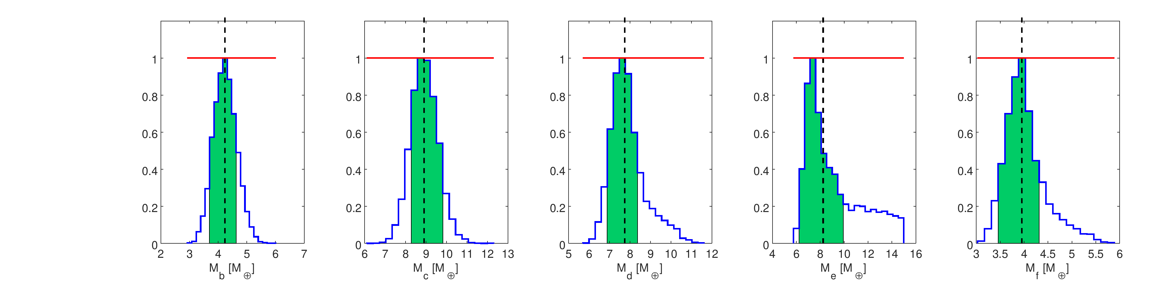
Figure 14: Posterior distributions for the masses $M_{\mathrm{p}}$ of the planets composing the HD 108236 system. In each panel, the horizontal red line represents the flat prior imposed on $M_{\mathrm{p}}$, implying that $M_{\mathrm{p}}$ was set as a free parameter. The dashed black line marks the median of the distribution, while the green area shows the 68% highest posterior density credible interval.

6 Conclusions

We have presented the combined analysis of TESS and CHEOPS LCs of the HD 108236 multi-planet system, along with the characterisation of the host star. Our spectroscopic analysis confirmed that HD 108236 is a Sun-like star with $T_{\mathrm{eff}}=5660\pm 61$ K and $\log{g}=4.49\pm 0.11$, though it is slightly metal poor with a metallicity of [Fe/H]$=-0.28\pm 0.04$ dex. We estimated the stellar radius to be $R_{\star}=0.877\pm 0.008\,R_{\odot}$, and determined robust values for stellar mass and age by employing two sets of stellar isochrones and tracks, obtaining $M_{\star}=0.869_{-0.048}^{+0.050}\,M_{\odot}$ and $t_{\star}=6.7_{-5.1}^{+4.0}$ Gyr.

Four planets were identified in the TESS LCs of HD 108236 by D20. We complemented this analysis by adding three CHEOPS datasets, which were supposed to contain one further transit for each of these planets. Inspecting one of the datasets, we serendipitously discovered an unexpected transit-like feature with a depth of $\sim$400 ppm that we ascribed to a fifth planet, HD 108236 f. We derived the Bayesian evidence for a four- and five-planet model, finding that the latter was significantly favoured. The combined TESS and CHEOPS LC analysis led us to derive a likely period for HD 108236 f of $P_{\mathrm{f}}=29.54$ days. Within the context of searching for additional planets in the system, we also investigated the presence in the CHEOPS LCs of the tentative candidate with a period of 10.9113 days suggested by D20, but we could not find strong evidence supporting it.

Within the scenario comprising five planets, the combined analysis of the TESS and CHEOPS LCs resulted in system parameters in agreement with those of D20 for planets HD 108236 b to HD 108236 e. However, our results are more precise in terms of transit depths (due to the high quality of the CHEOPS photometry), planetary radii (due to the improved measured transit depths and stellar radius), and ephemerides (due to the longer baseline covered by the data). We further ran a dynamical stability analysis of the system, finding that stability is maximised when the eccentricities of all planets are smaller than about 0.1. Comparing the results obtained from the analysis of the TESS and CHEOPS LCs separately, we found that, for a $V$ $\sim$ 9 mag solar-like star considering a transit signal with a depth of $\sim$500 ppm (i.e. a $\sim$2 $R_{\oplus}$ mini-Neptune transiting a solar-like star), one CHEOPS transit returns data with a quality comparable to that obtained from about eight TESS transits.

The refined ephemerides we obtained from the LC analysis will allow more accurate planning of follow-up observations of this system. HD 108236 will be visible with CHEOPS again, with an efficiency higher than 50%, between March and June 2021, at which point the planetary transit timings will be predictable with uncertainties of just a few minutes. Instead, by employing the $T_{0}$ and $P$ values from D20, based on just $\sim$ 2 months of TESS observations, the uncertainties on the transit timings would have been of the order of a couple of hours. We also evaluated the timescales after which the uncertainties on the transit timings become greater than 30 minutes, following the criterion in Dragomir et al. (2020). We concluded that our ephemerides remain fresh on timescales ranging between $\sim$ 4 years (planet f) and $\sim$ 12 years (planet e) from the last CHEOPS observations.

TESS will observe HD 108236 again during the extended mission in April 2021 within one sector of observations. If combined with the already available observations, and assuming TESS will collect the exact same amount of transits for each planet per sector, the entire TESS dataset will help reduce the uncertainties on the planetary radii by a factor of $\sim$ 1.2. This would imply reaching the same level of precision as our TESS+CHEOPS approach for planets c and d; however, the results presented here with the contribution of CHEOPS data would still guarantee a better precision on the radii of planets b, e, and f by at least a factor of $\sim$ 1.2. Future CHEOPS observations will therefore lead to further improvements in the measurement of the planetary radii, even more so compared to what was obtained through the TESS extended mission data. Furthermore, future CHEOPS data on this system will be important for looking for and measuring the TTVs that provide key information regarding the system dynamics as well as a measurement of the planetary masses, independent of what given by the RV method.

We finally used the derived system parameters and a planetary atmospheric evolutionary framework to constrain the planetary masses, finding that HD 108236 b and HD 108236 c should have an Earth-like density, while the outer planets are likely to host a low mean molecular weight atmosphere. The brightness and age of the host star make this an ideal target for measuring planetary masses using high-precision RV measurements. The expected semi-amplitudes of the RV variations are within reach of instruments such as HARPS (Mayor et al., 2003) and ESPRESSO (Pepe et al., 2020) spectrographs. This will enable us to check the impact of the modelling assumptions and to perform more detailed planetary atmospheric evolution modelling, aimed at deriving the past and future evolution of the system.

Appendix A Initial priors of the LC analyses.

Table 11: Initial priors used in our fits. $\mathcal{N}(\mu_{0},\sigma_{0})$ denotes a Normal (Gaussian) prior with mean $\mu_{0}$ and standard deviation $\sigma_{0}$, while $\mathcal{U}(a_{0},b_{0})$ denotes a uniform prior, whose bounds are $a_{0}$ and $b_{0}$. $\rho_{\star}$ is expressed in g/cm³, $T_{0}$ in BJD, $P$ in days. All other quantities are dimensionless.

Parameter	Prior
$\rho_{\star}$	$\mathcal{N}(1.82,0.12)$
$q_{1,{\mathrm{TESS}}}$	$\mathcal{N}(0.34,0.05)$
$q_{2,{\mathrm{TESS}}}$	$\mathcal{N}(0.27,0.05)$
$q_{1,{\mathrm{CHEOPS}}}$	$\mathcal{N}(0.46,0.05)$
$q_{2,{\mathrm{CHEOPS}}}$	$\mathcal{N}(0.32,0.05)$
Planet b
$\frac{R_{p}}{R_{\star}}$	$\mathcal{N}(0.016,0.005)$
$\frac{R_{p}+R_{\star}}{a}$	$\mathcal{N}(0.091,0.008)$
$\cos{i}$	$\mathcal{U}(0.,0.25)$
$T_{0}$	$\mathcal{N}(2458598.68,0.02)$
$P$	$\mathcal{N}(3.7955,0.0043)$
$\sqrt{e}\cos{\omega}$	$\mathcal{U}(-0.7,0.7)$
$\sqrt{e}\sin{\omega}$	$\mathcal{U}(-0.7,0.7)$
Planet c
$\frac{R_{p}}{R_{\star}}$	$\mathcal{N}(0.021,0.003)$
$\frac{R_{p}+R_{\star}}{a}$	$\mathcal{N}(0.065,0.006)$
$\cos{i}$	$\mathcal{U}(0.,0.25)$
$T_{0}$	$\mathcal{N}(2458597.210,0.014)$
$P$	$\mathcal{N}(6.2036,0.0035)$
$\sqrt{e}\cos{\omega}$	$\mathcal{U}(-0.7,0.7)$
$\sqrt{e}\sin{\omega}$	$\mathcal{U}(-0.7,0.7)$
Planet d
$\frac{R_{p}}{R_{\star}}$	$\mathcal{N}(0.026,0.004)$
$\frac{R_{p}+R_{\star}}{a}$	$\mathcal{N}(0.039,0.004)$
$\cos{i}$	$\mathcal{U}(0.,0.25)$
$T_{0}$	$\mathcal{N}(2458599.688,0.011)$
$P$	$\mathcal{N}(14.1757,0.0079)$
$\sqrt{e}\cos{\omega}$	$\mathcal{U}(-0.9,0.9)$
$\sqrt{e}\sin{\omega}$	$\mathcal{U}(-0.9,0.9)$
Planet e
$\frac{R_{p}}{R_{\star}}$	$\mathcal{N}(0.032,0.003)$
$\frac{R_{p}+R_{\star}}{a}$	$\mathcal{N}(0.031,0.002)$
$\cos{i}$	$\mathcal{U}(0.,0.25)$
$T_{0}$	$\mathcal{N}(2458606.160,0.012)$
$P$	$\mathcal{N}(19.591,0.013)$
$\sqrt{e}\cos{\omega}$	$\mathcal{U}(-0.9,0.9)$
$\sqrt{e}\sin{\omega}$	$\mathcal{U}(-0.9,0.9)$
Planet f
$\frac{R_{p}}{R_{\star}}$	$\mathcal{N}(0.020,0.006)$
$\frac{R_{p}+R_{\star}}{a}$	$\mathcal{N}(0.024,0.004)$
$\cos{i}$	$\mathcal{U}(0.,0.25)$
$T_{0}$	$\mathcal{N}(2458616.034,0.058)$
$P$	$\mathcal{N}(29.542,0.016)$
$\sqrt{e}\cos{\omega}$	$\mathcal{U}(-0.9,0.9)$
$\sqrt{e}\sin{\omega}$	$\mathcal{U}(-0.9,0.9)$