Verifying Global Optimality of Candidate Solutions to Polynomial
Optimization Problems using a Determinant Relaxation Hierarchy

Abstract

We propose an approach for verifying that a given feasible point for a polynomial optimization problem is globally optimal. The approach relies on the Lasserre hierarchy and the result of Lasserre regarding the importance of the convexity of the feasible set as opposed to that of the individual constraints. By focusing solely on certifying global optimality and relaxing the Lasserre hierarchy using necessary conditions for positive semidefiniteness based on matrix determinants, the proposed method is implementable as a computationally tractable linear program. We demonstrate this method via application to several instances of polynomial optimization, including the optimal power flow problem used to operate electric power systems.

I INTRODUCTION

Consider a polynomial optimization problem

$$\begin{array}[]{ll}\inf_{x}&f(x):=\sum_{\alpha}f_{\alpha}x^{\alpha}\\ \mathrm{s.t.}&g_{i}(x):=\sum_{\alpha}g_{i,\alpha}x^{\alpha}\geqslant 0,\quad i=1,\ldots,m\end{array}$$ (1)

where we use the multi-index notation $x^{\alpha}:=x_{1}^{\alpha_{1}}\cdots x_{n}^{\alpha_{n}}$ for $x\in{\mathbb{R}}^{n}$, $\alpha\in{\mathbb{N}}^{n}$, and where the data are polynomials $f,g_{1},\ldots,g_{m}\in{\mathbb{R}}[x]$ so that in the above sums only a finite number of coefficients $f_{\alpha}$ and $g_{i,\alpha}$ are nonzero. We will use the notation $|\alpha|:=\sum_{k=1}^{n}\alpha_{k}$.

Polynomial optimization problems (1) are generally non-convex and may therefore have multiple local and global optima. Local optima are feasible points for which no nearby point has a lower-cost objective value. Global optima are feasible points which have the lowest objective value among all feasible points. Many applications require (or at least benefit from) finding a global optimum to (1). Provably obtaining a global optimum is often accomplished by:

1. Using a local solver to compute a locally optimal point that is a candidate for being a global optimum.

2. Computing the optimality gap based on the difference between the objective value of the candidate point and the lower bound on the objective value provided by a convex relaxation of (1).

The candidate point is declared to be globally optimal if the optimality gap is sufficiently small. When the optimality gap is not sufficiently small, typical global optimization methods attempt to close the optimality gap by applying a variety of techniques for tightening the relaxation and obtaining a better local optimum [1, 2].

For certain polynomial optimization problems, especially those modeling physical systems, it is often straightforward to obtain high-quality local optima due to preexisting knowledge of appropriate initializations for local solvers. Consider, for instance, the optimal power flow (OPF) problem used in the operation of electric power systems [3, 4]. OPF problems are known to be NP-hard [5, 6]. Accordingly, there exist various test cases that challenge many solution algorithms [7, 8, 9, 10]. However, despite this challenging worst-case complexity, local solvers with physically justified initializations find the global optima for many practical OPF problems as verified by the small or zero optimality gaps obtained via a variety of convex relaxation techniques [11, 12, 13, 14, 15, 16]. (See [17] for a detailed survey.) Moreover, appropriately initialized local solvers can be significantly more computationally tractable than the convex relaxations used to certify global optimality [18, 19]. Thus, the computational effort for provably obtaining a globally optimal solution is often dominated by the time spent solving relaxations which show that a candidate feasible point from a local solver is, in fact, globally optimal.

Such problems motivate the development of methods for checking whether a given feasible point (e.g., the output of a local solver) is globally optimal. In contrast to convex relaxation techniques, whose objective values provide bounds on the potential suboptimality associated with a local solution, this paper solely focuses on methods for certifying whether a given feasible point is globally optimal. This less ambitious aim in comparison to existing convex relaxation techniques facilitates computational advantages for the proposed approach. Specifically, we reduce the problem of certifying global optimality of a candidate point to testing feasibility of a linear program.

Our proposed approach is particularly useful in settings that require the solution of many polynomial optimization problems. When applied as a screening step, our approach limits the need for explicitly solving computationally intensive relaxations to problems for which the candidate point and the selected relaxation result in a non-zero optimality gap. This allows us to leverage much of the extensive theoretical work regarding relaxations of polynomial optimization problems that has heretofore been practically limited by computational challenges associated with existing conic optimization solvers.

We close the introduction by reviewing two papers that aim to certify global optimality of polynomial optimization problems. Reviews of the specific relaxation techniques we employ will be presented in the following section.

The approach in [20] finds a objective function $\hat{f}$ for which a candidate point, $\hat{x}$, is globally optimal:

$$\begin{array}[]{ll}\inf_{\hat{f}}&\|f-\hat{f}\|\\ \mathrm{s.t.}&\hat{f}(x)-\hat{f}(\hat{x})\geqslant 0,~{}\forall x\in\mathcal{K}\end{array}$$ (2)

where $\mathcal{K}$ denotes the feasible space defined by the constraints in (1) and $\|\cdot\|$ is, for instance, the 2-norm of the coefficients. If the optimal objective value of (2) is equal to zero, then $\hat{x}$ is globally optimal. If not, then the solution of (2) provides insight into how far $\hat{x}$ is from the global optimum. Specifically, the solution to (2) yields an objective function, as close to the original objective function as possible, for which the candidate point $\hat{x}$ is globally optimal. In order to solve (2), [20] proposes to replace the non-negativity constraint using Putinar’s Positivstellensatz. The drawback of this approach is that it is a priori as computationally costly as actually computing a global solution.

In [21], another related approach provides a sufficient (but not necessary) condition for certifying global optimality of a candidate point by evaluating whether the point satisfies the Karush-Kuhn-Tucker (KKT) conditions [22, 23] for a relaxation. Assuming certain constraint qualification conditions (e.g., Slater’s condition), a local solution necessarily satisfies the KKT conditions for the non-convex polynomial optimization problem (1). If the local solution additionally satisfies the KKT conditions for a convex relaxation of (1), then the local solution is, in fact, a global optimum. The approach in [21] specifically tests whether a local solution to an OPF problem satisfies the KKT conditions for the Shor relaxation [24], which is equivalent, in the case of OPF problems, to the first-order moment/sum-of-squares relaxation in the Lasserre hierarchy to be discussed below. While explicitly computing the Shor relaxation requires the solution of a semidefinite program, evaluating whether the primal/dual variables obtained from a local solver satisfy the Shor relaxation’s KKT conditions only requires a single Cholesky factorization of a sparse matrix and a vector dot product. Thus, certifying global optimality by evaluating the condition in [21] is up to two orders of magnitude faster than explicitly solving the Shor relaxation for various OPF test cases, even after applying advanced techniques for improving the relaxation’s computational tractability [25, 26]. The approach proposed in the remainder of this paper can be viewed as an extension of the condition in [21] to exploit certain tighter relaxations, specifically, higher-order moment/sum-of-squares relaxations in the Lasserre hierarchy.

The remainder of paper is organized as follows. Section II presents the proposed approach. Section III applies the approach to several polynomial optimization problems including an instance of the optimal power flow problem. Section IV concludes the paper and proposes avenues for future research.

II Approach

In 2001, the Lasserre hierarchy [27, 28] (see also [29, 30]) was proposed to find global solutions to polynomial optimization problems. It is also known as moment/sum-of-squares hierarchy in reference to the primal moment hierarchy and the dual sum-of-squares hierarchy. Its global convergence is guaranteed by Putinar’s Positivstellensatz [31] proven in 1993. Typically, if one of the constraints is a ball $x_{1}^{2}+\ldots+x_{n}^{2}\leqslant 1$, then the sequence of lower bounds provided by the hierarchy converges to the global infimum of the polynomial optimization problem. In addition, there is zero duality at all relaxation orders [32].

The moment problem of order $d$ is defined as

$$\begin{array}[]{ll}\inf_{y}&L_{y}(f)\\ \mathrm{s.t.}&y_{0}=1\\ &M_{d}(y)\succcurlyeq 0\\ &M_{d-k_{i}}(g_{i}y)\succcurlyeq 0,\quad i=1,\ldots,m\end{array}$$ (3)

where $\succcurlyeq 0$ denotes positive semidefiniteness, and where the Riesz functional, the moment matrix, and the localizing matrices are respectively defined by

$$\begin{array}[]{l}L_{y}(f):=\sum_{\alpha}f_{\alpha}y_{\alpha}\\[5.69046pt] M_{d}(y):=(y_{\alpha+\beta})_{|\alpha|,|\beta|\leqslant d}\\[5.69046pt] M_{d-k_{i}}(g_{i}y):=(\sum_{\gamma}g_{i,\gamma}y_{\alpha+\beta+\gamma})_{|\alpha|,|\beta|\leqslant d-k_{i}}\\[5.69046pt] k_{i}:=\max\{\lceil|\alpha|/2\rceil~{}\text{s.t.}~{}g_{i,\alpha}\neq 0\}.\end{array}$$ (4)

Above, $\lceil\cdot\rceil$ denotes the ceiling of a real number. Note that the relaxation order $d$ must be greater than or equal to $d^{\text{min}}:=\max_{i}k_{i}$. See Section III for an illustrative example of a second-order moment/sum-of-squares relaxation of a quadratically constrained quadratic program corresponding to a two-bus OPF problem.

Our approach extends a relaxation technique proposed in [33] that leverages theory developed in [34, 35] regarding the importance of the convexity of the feasible space rather than its algebraic representation. The technique in [33] further relaxes the Shor relaxation [24] using necessary conditions for positive semidefiniteness based on matrix determinants. Specifically, the approach in [33] exploits the fact that a symmetric matrix is positive semidefinite if and only if all its principal minors (i.e., the determinants of its principal submatrices) are non-negative [36]. Extending this approach to the Lasserre hierarchy (3) yields

$$\begin{array}[]{ll}\inf_{y}&L_{y}(f)\\ \mathrm{s.t.}&y_{0}=1\\ &\det_{I}(M_{d}(y))\geqslant 0\\ &\quad\text{for all~{}}I=\{1\},\{2\},\ldots,\{1,2\},\\ &\{1,3\},\ldots,\{1,2,\ldots,n_{0}\},\\ &\det_{J_{i}}(M_{d-k_{i}}(g_{i}y))\geqslant 0\\ &\quad\text{for all~{}}J_{i}=\{1\},\{2\},\ldots,\{1,2\},\\ &\{1,3\},\ldots,\{1,2,\ldots,n_{i}\},\\ &\qquad i=1,\ldots,m,\end{array}$$ (5)

where $n_{0}:=\frac{\left(n+d\right)!}{n!\,d!}$ is the size of the matrix $M_{d}(y)$, $n_{i}:=\frac{\left(n+d-k_{i}\right)!}{n!\,\left(d-k_{i}\right)!}$ is the size of the matrix $M_{d-k_{i}}(y)$, and $\det_{I}$ denotes the principal minor corresponding to the index $I$ (i.e., the determinant of the submatrix whose rows and columns are indexed by $I$), likewise for $\det_{J_{i}}$.

To derive our approach, we exploit the KKT conditions of the formulation (5). To express these conditions, let $\lambda$ denote the KKT multiplier associated with the constraint $y_{0}=1$. Let $\lambda_{0,I}$ denote the KKT multiplier associated with the constraint $\det_{I}(M_{d}(y))\geqslant 0$. Let $\lambda_{i,J_{i}}$ denote the KKT multiplier associated with the constraint $\det_{J_{i}}(M_{d-k_{i}}(g_{i}y))\geqslant 0$. The KKT conditions of (5) are

$$\begin{array}[]{l}\nabla L_{y}(f)-\lambda e_{1}-\sum\limits_{I}\lambda_{0,I}\nabla_{y}\det_{I}(M_{d}(y))+\ldots\\ -\sum\limits_{i=1}^{m}\sum\limits_{J_{i}}\lambda_{i,J_{i}}\nabla_{y}\det_{J_{i}}(M_{d-k_{i}}(g_{i}y))=0,\\ y_{0}=1,\\ \det_{I}(M_{d}(y))\geqslant 0,\\ \det_{J_{i}}(M_{d-k_{i}}(g_{i}y))\geqslant 0,\quad i=1,\ldots,m,\\ \lambda_{0,I}\geqslant 0,\\ \lambda_{i,J_{i}}\geqslant 0,\quad i=1,\ldots,m,\\ \det_{I}(M_{d}(y))\lambda_{0,I}=0,\\ \det_{J_{i}}(M_{d-k_{i}}(g_{i}y))\lambda_{i,J_{i}}=0,\quad i=1,\ldots,m.\end{array}$$ (6)

We have that $\nabla\det(M)=\text{co}(M)$ where the comatrix $\text{co}(M)$ is defined by $\text{co}(M)_{i,j}:=(-1)^{i+j}\det(M^{(i,j)})$; $M^{(i,j)}$ is the matrix $M$ where row $i$ and column $j$ have been removed. Let $\text{co}_{I}(\cdot)$ denote the comatrix of the submatrix whose rows and columns are indexed by a subset of indices $I$. Below, we will consider matrices $B_{\alpha}$ and $C_{i,\alpha}$ such that the moment and localizing matrices are as follows:

$$M_{d}(y)=:\sum_{|\alpha|\leqslant 2d}B_{\alpha}y_{\alpha}$$ (7)

and

$$M_{d-k_{i}}(g_{i}y)=:\sum_{|\alpha|\leqslant 2(d-k_{i})}C_{i,\alpha}\,y_{\alpha}.$$ (8)

The KKT conditions are then

$$\begin{array}[]{l}f_{\alpha}-\lambda e_{1}-\sum\limits_{I}\lambda_{0,I}\,\text{trace}(\text{co}_{I}(M_{d}(y))B_{I,\alpha})+\ldots\\ -\sum\limits_{i=1}^{m}\sum\limits_{J_{i}}\lambda_{i,J_{i}}\text{trace}(\text{co}_{J_{i}}(M_{d-k_{i}}(g_{i}y))C_{i,J_{i},\alpha})=0,\\ y_{0}=1,\\ \det_{I}(M_{d}(y))\geqslant 0,\\ \det_{J_{i}}(M_{d-k_{i}}(g_{i}y))\geqslant 0,\quad i=1,\ldots,m,\\ \lambda_{0,I}\geqslant 0,\\ \lambda_{i,J_{i}}\geqslant 0,\quad i=1,\ldots,m,\\ \det_{I}(M_{d}(y))\lambda_{0,I}=0,\\ \det_{J_{i}}(M_{d-k_{i}}(g_{i}y))\lambda_{i,J_{i}}=0,\quad i=1,\ldots,m.\end{array}$$ (9)

If we substitute $y$ using the feasible point $\hat{x}$, i.e., by taking $\hat{y}:=(\hat{x}^{\alpha})_{|\alpha|\leqslant 2d}$, the KKT conditions reduce to a linear feasibility problem, that is

$$\begin{array}[]{l}f_{\alpha}-\lambda e_{1}-\sum\limits_{I}\lambda_{0,I}\text{trace}(\text{co}_{I}(M_{d}(\hat{y}))B_{I,\alpha})+\ldots\\ -\sum\limits_{i=1}^{m}\sum\limits_{J_{i}}\lambda_{i,J_{i}}\text{trace}(\text{co}_{J_{i}}(M_{d-k_{i}}(g_{i}\hat{y}))C_{i,J_{i},\alpha})=0,\\ \lambda_{0,I}\geqslant 0,\\ \lambda_{i,J_{i}}\geqslant 0,\quad i=1,\ldots,m,\\ \hat{y}_{2\alpha}\,\lambda_{0,\{\alpha\}}=0,\quad\forall|\alpha|\leqslant d,\\[2.84544pt] (\sum\limits_{\beta}g_{i,\beta}\,\hat{y}_{2\alpha+\beta})\,\lambda_{i,\{\alpha\}}=0,\quad\forall|\alpha|\leqslant d-k_{i},\\ i=1,\ldots,m.\end{array}$$ (10)

Observe that all the determinants are equal to zero, except when the index sets $I$ and $J_{i}$ are singletons (i.e., $I=J_{i}=\{\alpha\}$ where $\alpha\in\mathbb{N}^{n}$). In that case, the determinant is simply equal to a diagonal term of the matrix.

Any point that satisfies (10) provides values for dual variables that, in combination with the primal variables $\hat{y}$ obtained from the candidate solution $\hat{x}$, satisfy the KKT conditions corresponding to a convex relaxation of (1). Hence, any feasible point for (10) certifies global optimality of the candidate feasible point $\hat{x}$ for the polynomial optimization problem (1).

Since all values $\hat{y}$ are fixed, we emphasize that (10) is linear in the KKT multipliers $\lambda$, $\lambda_{0,I}$, and $\lambda_{0,J_{i}}$. Thus, the KKT conditions (10) can be verified using a linear programming solver, which is significantly more computationally tractable than solving the KKT conditions for the relaxation (9) with both primal variables $y$ and dual variables $\lambda$, $\lambda_{0,I}$, and $\lambda_{0,J_{i}}$ allowed to vary (a complementarity problem).

III Numerical experiments

We implemented the algorithms with Matlab R2020a. We used Gloptipoly 3 to obtain the Lasserre hierarchy formulation. As for solving the KKT conditions, we used the LINPROG and LSQLIN solver provided by Matlab. The optimality tolerance of both solvers are set to $10^{-8}$.

III-A Univariate example

Consider the following polynomial optimization problem represented in Figure 1 with a local minimum at $-2$ and a global minimum at $2$:

$$\inf_{x\in\mathbb{R}}~{}~{}~{}\frac{1}{4}x^{4}+\frac{1}{8}x^{3}-2x^{2}-\frac{3}{2}x+7~{}~{}~{}\text{s.t.}~{}~{}~{}-x^{2}+5\geqslant 0.$$ (11)

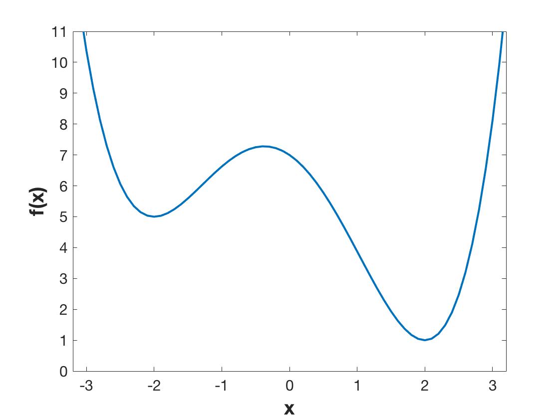
Figure 1: Univariate example

The second-order moment relaxation reads:

$$\begin{array}[]{ll}\inf_{y\in\mathbb{R}^{5}}&\frac{1}{4}y_{4}+\frac{1}{8}y_{3}-2y_{2}-\frac{3}{2}y_{1}+7y_{0}\\[11.38092pt] \text{s.t.}&\left\{\begin{array}[]{l}y_{0}=1,\\ \begin{pmatrix}y_{0}&y_{1}&y_{2}\\ y_{1}&y_{2}&y_{3}\\ y_{2}&y_{3}&y_{4}\\ \end{pmatrix}\succcurlyeq 0,\\[15.00002pt] \begin{pmatrix}-y_{2}+5y_{0}&-y_{3}+5y_{1}\\ -y_{3}+5y_{1}&-y_{4}+5y_{2}\\ \end{pmatrix}\succcurlyeq 0.\end{array}\right.\end{array}$$ (12)

Using the determinant condition for positive semidefiniteness as in (5), an equivalent formulation of the second-order moment relaxation is as follows:

$$\inf_{y\in\mathbb{R}^{5}}~{}~{}~{}\frac{1}{4}y_{4}+\frac{1}{8}y_{3}-2y_{2}-\frac{3}{2}y_{1}+7y_{0}$$ (13)

subject to

$$\left\{\begin{array}[]{l}y_{0}=1,\\[2.84526pt] y_{0}\geqslant 0,~{}y_{2}\geqslant 0,~{}y_{4}\geqslant 0,\\[2.84526pt] y_{0}y_{2}-y_{1}^{2}\geqslant 0,~{}y_{0}y_{4}-y_{2}^{2}\geqslant 0,~{}y_{2}y_{4}-y_{3}^{2}\geqslant 0,\\[2.84526pt] y_{0}(y_{2}y_{4}-y_{3}^{2})-y_{1}(y_{1}y_{4}-y_{3}y_{2})\\ +y_{2}(y_{1}y_{3}-y_{2}^{2})\geqslant 0,\\[2.84526pt] -y_{2}+5y_{0}\geqslant 0,~{}-y_{4}+5y_{2}\geqslant 0,\\[2.84526pt] (-y_{2}+5y_{0})(-y_{4}+5y_{2})-(-y_{3}+5y_{1})^{2}\geqslant 0.\end{array}\right.$$ (14)

Observe that each constraint taken separately may be non-convex, yet together they yield a convex region. We then define the following Lagrangian:

$$\begin{array}[]{cc}\mathcal{L}(y,\lambda,\lambda_{0},\lambda_{1}):=\frac{1}{4}y_{4}+\frac{1}{8}y_{3}-2y_{2}-\frac{3}{2}y_{1}\\ +7y_{0}+(1-y_{0}){\lambda}-y_{0}{\lambda_{0,\{1\}}}-y_{2}{\lambda_{0,\{2\}}}\\ -y_{4}{\lambda_{0,\{3\}}}-(y_{0}y_{2}-y_{1}^{2}){\lambda_{0,\{1,2\}}}\\ -(y_{0}y_{4}-y_{2}^{2}){\lambda_{0,\{1,3\}}}-(y_{2}y_{4}-y_{3}^{2}){\lambda_{0,\{2,3\}}}\\ -[y_{0}(y_{2}y_{4}-y_{3}^{2})-y_{1}(y_{1}y_{4}-y_{3}y_{2})\\ +y_{2}(y_{1}y_{3}-y_{2}^{2})]{\lambda_{0,\{1,2,3\}}}+\\ -(-y_{2}+5y_{0}){\lambda_{1,\{1\}}}-(-y_{4}+5y_{2}){\lambda_{1,\{2\}}}+\\ -[(-y_{2}+5y_{0})(-y_{4}+5y_{2})\\ -(-y_{3}+5y_{1})^{2}]{\lambda_{1,\{1,2\}}}.\end{array}$$ (15)

The KKT conditions that need to be met by the dual multipliers of (13)–(14) are thus given by:

$$\left\{\begin{array}[]{l}7-{\lambda}-{\lambda_{0,\{1\}}}-y_{2}{\lambda_{0,\{1,2\}}}-y_{4}{\lambda_{0,\{1,3\}}}\\ -(y_{2}y_{4}-y_{3}^{2}){\lambda_{0,\{1,2,3\}}}=0,\\[5.69046pt] -3/2+2y_{1}{\lambda_{0,\{1,2\}}}\\ -(-2y_{1}y_{4}+2y_{3}y_{2}){\lambda_{0,\{1,2,3\}}}\\ +10(-y_{3}+5y_{1}){\lambda_{1,\{1,2\}}}=0,\\[5.69046pt] -2-{\lambda_{0,\{2\}}}-y_{0}{\lambda_{0,\{1,2\}}}+2y_{2}^{2}{\lambda_{0,\{1,3\}}}\\ -y_{4}{\lambda_{0,\{2,3\}}}+(-y_{0}y_{4}-y_{1}y_{3}-y_{1}y_{3}\\ +3y_{2}^{2}){\lambda_{0,\{1,2,3\}}}+{\lambda_{1,\{1\}}}-5{\lambda_{1,\{2\}}}\\ +(-y_{4}+10y_{2}-25y_{0}){\lambda_{1,\{1,2\}}}=0,\\[11.38092pt] 1/8+2y_{3}{\lambda_{0,\{2,3\}}}\\ -(-2y_{0}y_{3}+2y_{1}y_{2}){\lambda_{0,\{1,2,3\}}}\\ -(-2y_{3}+10y_{1}){\lambda_{1,\{1,2\}}}=0,\\[11.38092pt] 1/4-{\lambda_{0,\{3\}}}-y_{0}{\lambda_{0,\{1,3\}}}-y_{2}{\lambda_{0,\{2,3\}}}\\ -(y_{0}y_{2}-y_{1}^{2}){\lambda_{0,\{1,2,3\}}}+{\lambda_{1,\{2\}}}\\ +(-y_{2}+5y_{0}){\lambda_{1,\{1,2\}}}=0,\\[5.69046pt] {\lambda_{0,\{1\}}},~{}{\lambda_{0,\{2\}}},~{}{\lambda_{0,\{3\}}},~{}{\lambda_{0,\{1,2\}}},\\ {\lambda_{0,\{1,3\}}},~{}{\lambda_{0,\{2,3\}}},~{}{\lambda_{0,\{1,2,3\}}}\geqslant 0,\\ {\lambda_{1,\{1\}}},~{}{\lambda_{1,\{2\}}},~{}{\lambda_{1,\{1,2\}}}\geqslant 0,\\[5.69046pt] y_{0}{\lambda_{0,\{1\}}}=y_{2}{\lambda_{0,\{2\}}}=y_{4}{\lambda_{0,\{3\}}}=0,\\[5.69046pt] {\lambda_{1,\{1\}}}(-y_{2}+5y_{0})={\lambda_{1,\{2\}}}(-y_{4}+5y_{2})=0.\end{array}\right.$$ (16)

We next check whether $x=-2$ or $x=2$ are global solutions. In order to do so, we plug $x$ into the primal variable $y$ in the above system, i.e., $y_{i}:=x^{i}$, and see whether there exists a feasible set of dual variables. If there exists feasible dual variables, then the point $x$ is a global solution. If not, then we may need to increase the order of the hierarchy and try again. In order to check for linear feasibility, we respectively minimize the $\ell_{1}$ and $\ell_{2}$ norms of the equality constraints, subject to the non-negativity constraints of the dual multipliers. The $\ell_{1}$ norm results in a linear program while the $\ell_{2}$ norm results in a convex quadratic optimization problem. The numerical results are shown in Table I. The local solution yields an infeasible linear system, while the global solution yields a linear system that is feasible with very high accuracy.

TABLE I: Global optimality check in univariate example

Solution	Optimality	$\ell_{1}$ norm	$\ell_{2}$ norm
$x=-2$	Local	$1.55\times 10^{0\hphantom{-}}$	$2.25\times 10^{0\hphantom{-}}$
$x=\hphantom{-}2$	Global	$2.30\times 10^{-7}$	$1.48\times 10^{-8}$

III-B Bivariate example

Consider the following polynomial optimization problem represented in Figure 2:

$$\inf_{x_{1},x_{2}\in\mathbb{R}}~{}~{}~{}2x_{1}^{3}+x_{1}^{2}+\frac{1}{4}x_{1}x_{2}+x_{2}^{2}-\frac{1}{2}x_{2}+\frac{1}{16}$$

$$\text{subject to}~{}~{}x_{1}^{2}+x_{2}^{2}\leq 1.$$ (17)

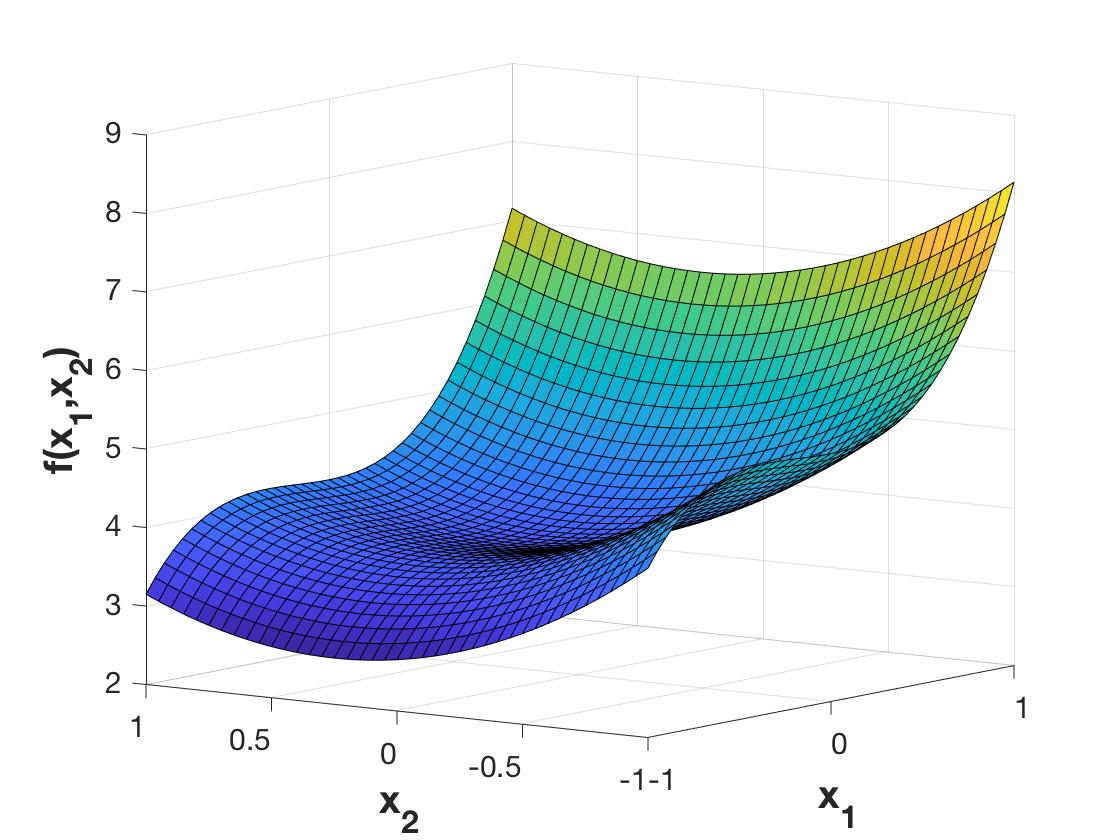
Figure 2: Bivariate example

The numerical results in Table II again show that the method correctly distinguishes the global solution from the local solution. The KKT system stemming from the second-order moment relaxation was used.

TABLE II: Global optimality check in bivariate example

Solution	Optimality	$\ell_{1}$ norm	$\ell_{2}$ norm
$x=(-0.036,0.254)$	Local	$1.99\times 10^{0\hphantom{-}}$	$3.68\times 10^{0\hphantom{-}}$
$x=(-0.992,0.125)$	Global	$1.75\times 10^{-4}$	$7.13\times 10^{-8}$

III-C Trivariate example

Consider the following polynomial optimization problem:

$$\inf_{x_{1},x_{2},x_{3}\in\mathbb{R}}\frac{2500}{13}x_{1}^{2}-\frac{12500}{13}x_{1}x_{3}-\frac{2500}{13}x_{1}x_{2}$$ (18)

subject to

$$\left\{\begin{array}[]{c}\frac{25}{26}x_{1}x_{2}-\frac{125}{26}x_{1}x_{3}-\frac{25}{26}x_{2}^{2}-\frac{25}{26}x_{3}^{2}-\frac{7}{2}=0\\[5.69054pt] \frac{125}{26}x_{1}x_{2}+\frac{25}{26}x_{1}x_{3}-\frac{125}{26}x_{2}^{2}-\frac{125}{26}x_{3}^{2}+\frac{7}{2}=0\\[5.69054pt] 0\leqslant\frac{25}{26}x_{1}^{2}-\frac{125}{26}x_{1}x_{3}-\frac{25}{26}x_{1}x_{2}\leqslant 6\\[5.69054pt] -4\leqslant\frac{25}{26}x_{1}x_{3}-\frac{125}{26}x_{1}x_{2}+\frac{125}{26}x_{1}^{2}\leqslant 4\\[5.69054pt] 0.9025\leqslant x_{1}^{2}\leqslant 1.1025\\[5.69054pt] 0.9025\leqslant x_{2}^{2}+x_{3}^{2}\leqslant 1.1025\end{array}\right.$$ (19)

This problem corresponds to the two-bus alternating current optimal power flow problem in Figure 3 from [7].

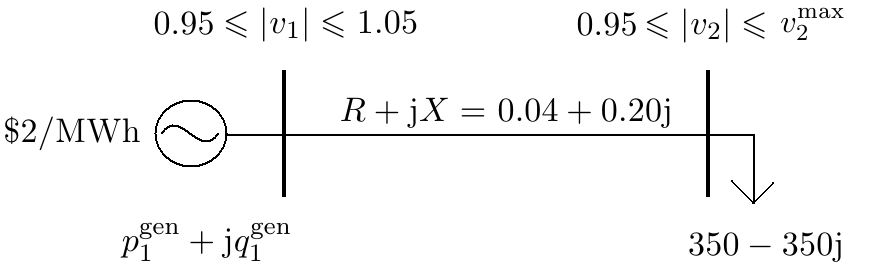
Figure 3: WB2 2-bus system

The feasible region of the polynomial optimization problem is represented in Figure 4, along with a local solution (blue square) and a global solution (green star).

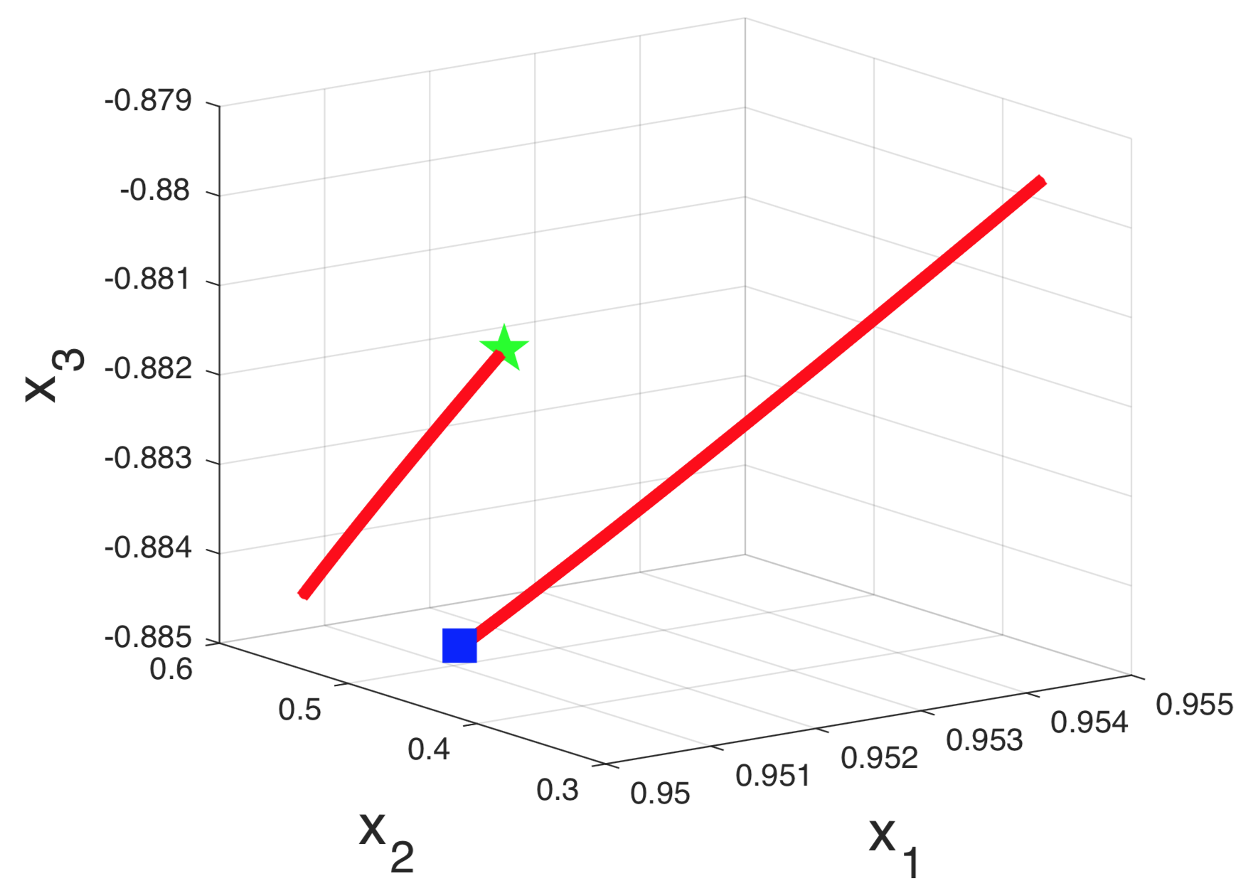
Figure 4: Trivariate example

The numerical results in Table III show that the method is able to distinguish between the local and global solutions, albeit less strikingly than in the univariate and bivariate examples. We attribute this to the proximity between the local and global solutions, which are taken from the test case archive. Their objective values are also close: the objective values of the local and global solutions are $905.73$ and $877.78$, respectively (a 3.2% difference). We used the KKT system stemming from the second-order moment relaxation, consistent with the empirical finding in [37, 38] that this relaxation is often tight in the context of power systems.

TABLE III: Global optimality check in trivariate example

Solution	Optimality	$\ell_{1}$ norm	$\ell_{2}$ norm
$x=(.950,.413,-.884)$	Local	$7.21\times 10^{-2}$	$2.96\times 10^{-3}$
$x=(.952,.570,-.882)$	Global	$5.31\times 10^{-3}$	$9.93\times 10^{-6}$

We conclude this section with the runtimes in Table IV. The runtimes are the average of 5 repeated experiments. One can see that there is a significant speed-up, by at least an order of magnitude, when checking for global optimality instead of computing a global solution. We do not report the time taken to setup the linear program and the semidefinite program, both of which could be reduced with a more sophisticated implementation.

TABLE IV: Runtimes (in seconds)

Problem	SDP	$\ell_{1}$ norm	$\ell_{2}$ norm
Univariate	$0.960$	$0.042$	$0.044$
Bivariate	$0.922$	$0.032$	$0.042$
Trivariate	$2.068$	$0.050$	$0.706$

IV Conclusion

We have proposed a method for verifying global optimality by checking for the feasibility of a linear system of equations. We have demonstrated the proof of concept on several small examples of polynomial optimization problems. A topic of further investigation is to exploit sparsity in order to make the approach tractable on larger optimal power flow instances. One could use techniques involving chordal graphs as was done in [15], which enabled the application of the Lasserre hierarchy to large-scale instances. Since global solutions were extracted in many instances within minutes, it is reasonable to believe that checking for global optimality should be possible with significantly faster runtimes. Another possible avenue for future research is to find another equivalent formulation of the Lasserre hierarchy whose KKT conditions would also lead to a tractable system for the dual multipliers (perhaps a second-order conic program).

References

- [1] C. A. Floudas, Deterministic Global Optimization: Theory, Methods and Applications, vol. 37. Springer Science & Business Media, 2013.
- [2] S. Gopinath, H. Hijazi, T. Weisser, H. Nagarajan, M. Yetkin, K. Sundar, and R. Bent, “Proving Global Optimality of ACOPF Solutions,” Electric Power Systems Research, vol. 189, p. 106688, 2020.
- [3] M. Carpentier, “Contribution à l’Étude du Dispatching Économique,” Bulletin de la Societe Francoise des Electriciens, vol. 8, pp. 431–447, 1962.
- [4] M. B. Cain, R. P. O’Neil, and A. Castillo, “History of Optimal Power Flow and Formulations (OPF Paper 1),” tech. rep., US Federal Energy Regulatory Commission, Dec. 2012.
- [5] D. Bienstock and A. Verma, “Strong NP-hardness of AC power flows feasibility,” Operations Research Letters, vol. 47, no. 6, pp. 494–501, 2019.
- [6] K. Lehmann, A. Grastien, and P. Van Hentenryck, “AC-Feasibility on Tree Networks is NP-Hard,” IEEE Transactions on Power Systems, vol. 31, pp. 798–801, Jan. 2016.
- [7] W. Bukhsh, A. Grothey, K. McKinnon, and P. Trodden, “Local Solutions of the Optimal Power Flow Problem,” IEEE Transactions on Power Systems, vol. 28, pp. 4780––4788, 2013.
- [8] S. Babaeinejadsarookolaee, A. Birchfield, R. D. Christie, C. Coffrin, C. L. DeMarco, R. Diao, M. Ferris, S. Fliscounakis, S. Greene, R. Huang, C. Josz, R. Korab, B. C. Lesieutre, J. Maeght, D. Molzahn, T. J. Overbye, P. Panciatici, B. Park, J. Snodgrass, and R. D. Zimmerman, “The Power Grid Library for Benchmarking AC Optimal Power Flow Algorithms,” August 2019. arXiv:1908.02788.
- [9] B. Kocuk, S. S. Dey, and X. A. Sun, “Inexactness of SDP Relaxation and Valid Inequalities for Optimal Power Flow,” IEEE Transactions on Power Systems, vol. 31, pp. 642–651, Jan. 2016.
- [10] M. R. Narimani, D. K. Molzahn, D. Wu, and M. L. Crow, “Empirical Investigation of Non-Convexities in Optimal Power Flow Problems,” American Control Conference (ACC), June 2018.
- [11] J. Lavaei and S. Low, “Zero Duality Gap in Optimal Power Flow Problem,” IEEE Transactions on Power Systems, vol. 27, pp. 92–107, Feb. 2012.
- [12] S. H. Low, “Convex Relaxation of Optimal Power Flow: Parts I & II,” IEEE Trans. Control Network Syst., vol. 1, pp. 15–27, Mar. 2014.
- [13] C. Coffrin, H. Hijazi, and P. Van Hentenryck, “The QC Relaxation: Theoretical and Computational Results on Optimal Power Flow,” IEEE Transactions on Power Systems, vol. 31, pp. 3008–3018, 2016.
- [14] D. K. Molzahn and I. A. Hiskens, “Sparsity-Exploiting Moment-Based Relaxations of the Optimal Power Flow Problem,” IEEE Transactions on Power Systems, vol. 30, pp. 3168–3180, Nov. 2015.
- [15] C. Josz and D. K. Molzahn, “Lasserre Hierarchy for Large Scale Polynomial Optimization in Real and Complex Variables,” SIAM Journal on Optimization, vol. 28, no. 2, pp. 1017–1048, 2018.
- [16] B. Kocuk, S. S. Dey, and X. A. Sun, “Matrix Minor Reformulation and SOCP-based Spatial Branch-and-Cut Method for the AC Optimal Power Flow Problem,” Mathematical Programming C, vol. 10, pp. 557–596, Dec. 2018.
- [17] D. K. Molzahn and I. A. Hiskens, “A Survey of Relaxations and Approximations of the Power Flow Equations,” Foundations and Trends in Electric Energy Systems, vol. 4, pp. 1–221, Feb. 2019.
- [18] A. Castillo and R. P. O’Neill, “Computational Performance of Solution Techniques Applied to the ACOPF (OPF Paper 5),” tech. rep., US Federal Energy Regulatory Commission, Jan. 2013.
- [19] R. Zimmerman, C. Murillo-Sánchez, and R. Thomas, “MATPOWER: Steady-State Operations, Planning, and Analysis Tools for Power Systems Research and Education,” IEEE Transactions on Power Systems, no. 99, pp. 1–8, 2011.
- [20] J. B. Lasserre, “Inverse Polynomial Optimization,” Mathematics of Operations Research, vol. 38, no. 3, pp. 418–436, 2013.
- [21] D. Molzahn, B. Lesieutre, and C. DeMarco, “A Sufficient Condition for Global Optimality of Solutions to the Optimal Power Flow Problem,” IEEE Transactions on Power Systems, vol. 29, pp. 978–979, Mar. 2014.
- [22] W. Karush, “Minima of Functions of Several Variables with Inequalities as Side Constraints,” Master’s thesis, University of Chicago, Department of Mathematics, Chicago, IL, 1939.
- [23] H. W. Kuhn and A. W. Tucker, “Nonlinear Programming,” Proceedings of the 2nd Berkeley Symposium on Mathematical Statistics and Probability, pp. 481–492, 1951.
- [24] N. Shor, “Quadratic Optimization Problems,” Soviet Journal of Computer and System Sciences, vol. 25, pp. 1–11, 1987.
- [25] R. Jabr, “Exploiting Sparsity in SDP Relaxations of the OPF Problem,” IEEE Transactions on Power Systems, vol. 27, pp. 1138–1139, May 2012.
- [26] D. Molzahn, J. Holzer, B. Lesieutre, and C. DeMarco, “Implementation of a Large-Scale Optimal Power Flow Solver Based on Semidefinite Programming,” IEEE Transactions on Power Systems, vol. 28, no. 4, pp. 3987–3998, 2013.
- [27] J. B. Lasserre, “Optimisation Globale et Théorie des Moments,” Comptes rendus de l’Académie des Sciences, Série I, vol. 331, pp. 929–934, 2000.
- [28] J. B. Lasserre, “Global Optimization with Polynomials and the Problem of Moments,” SIAM Journal on Optimization, vol. 11, pp. 796–817, 2001.
- [29] P. A. Parrilo, Structured Semidefinite Programs and Semialgebraic Geometry Methods in Robustness and Optimization. PhD thesis, California Institute of Technology, May 2000.
- [30] P. A. Parrilo, “Semidefinite Programming Relaxations for Semialgebraic Problems,” Mathematical Programming, vol. 96, pp. 293–320, 2003.
- [31] M. Putinar, “Positive Polynomials on Compact Semi-Algebraic Sets,” Indiana University Mathematics Journal, vol. 42, pp. 969–984, 1993.
- [32] C. Josz and D. Henrion, “Strong Duality in Lasserre’s Hierarchy for Polynomial Optimization,” Springer Optimization Letters, 2015.
- [33] H. Hijazi, C. Coffrin, and P. Van Hentenryck, “Polynomial SDP Cuts for Optimal Power Flow,” 19th Power Systems Computation Conference (PSCC), June 2016.
- [34] J. B. Lasserre, “On Representations of the Feasible Set in Convex Optimization,” Optimization Letters, vol. 4, no. 1, pp. 1–5, 2010.
- [35] J. B. Lasserre, “On Convex Optimization without Convex Representation,” Optimization Letters, vol. 5, no. 4, pp. 549–556, 2011.
- [36] J. E. Prussing, “The Principal Minor Test for Semidefinite Matrices,” Journal of Guidance, Control, and Dynamics, vol. 9, no. 1, pp. 121–122, 1986.
- [37] C. Josz, J. Maeght, P. Panciatici, and J. Gilbert, “Application of the Moment-SOS Approach to Global Optimization of the OPF Problem,” IEEE Transactions on Power Systems, vol. 30, pp. 463–470, Jan. 2015.
- [38] D. K. Molzahn and I. A. Hiskens, “Moment-Based Relaxation of the Optimal Power Flow Problem,” 18th Power Systems Computation Conference (PSCC), Aug. 2014.