Progressive Correspondence Pruning by Consensus Learning

Abstract

Correspondence selection aims to correctly select the consistent matches (inliers) from an initial set of putative correspondences. The selection is challenging since putative matches are typically extremely unbalanced, largely dominated by outliers, and the random distribution of such outliers further complicates the learning process for learning-based methods. To address this issue, we propose to progressively prune the correspondences via a local-to-global consensus learning procedure. We introduce a “pruning” block that lets us identify reliable candidates among the initial matches according to consensus scores estimated using local-to-global dynamic graphs. We then achieve progressive pruning by stacking multiple pruning blocks sequentially. Our method outperforms state-of-the-arts on robust line fitting, camera pose estimation and retrieval-based image localization benchmarks by significant margins and shows promising generalization ability to different datasets and detector/descriptor combinations.

1 Introduction

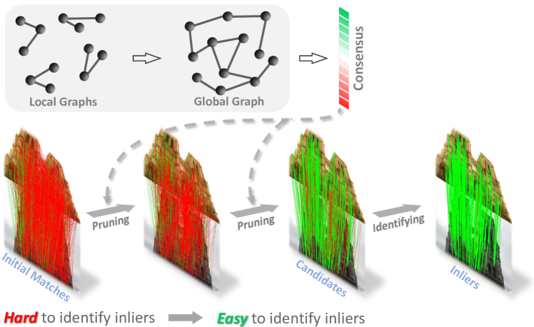
Figure 1: Progressive correspondence pruning via local-to-global consensus learning. Given initial correspondences (bottom-left image) with dominant outliers, correctly identifying inliers remains challenging. Instead of classifying correspondences in a one-shot fashion, we propose to gradually prune the correspondences to obtain a subset of reliable candidates based on correspondence consensus scores estimated from local-to-global graphs, encouraging accurate inlier identification.

Accurate pixel-wise correspondences act as a premise to tackle many important tasks in computer vision and robotics, such as Structure from Motion (SfM) [39], Simultaneous Location and Mapping (SLAM) [30], image stitching [7], visual localization [31], and virtual reality [41]. Unfortunately, feature correspondences established by off-the-shelf detector-descriptors  [26, 30, 28, 11] tend to be sensitive to challenging cross-image variations, such as rotations, scale changes, viewpoint changes, and illumination changes. Much recent research has therefore focused on correspondence selection [4, 27, 29], aiming to identify correct matches (inliers) while rejecting false ones (outliers).

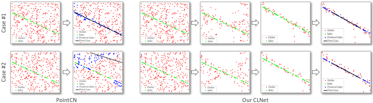
Figure 2: Robustness against different distributions of outliers. The inliers are the same in both cases while the outliers are randomly sampled. PointCN fails to find the correct line in the second case, showing its lack of robustness to the outlier distribution. By contrast, by gradually pruning the 2D points into reliable candidates for further line fitting, our method mitigates the effects of randomly-sampled outliers and consistently identifies the line.

In this context, deep learning has been utilized as a powerful solution [29, 48, 47, 40], typically casting correspondence selection as a per-match classification task, and adopting Multi-Layer Perceptrons (MLPs) to classify putative matches into inliers and outliers. However, the resulting learning problem is significantly complicated by the fact that the initial matches are general extremely unbalanced, with around $90\%$ of outliers [48](refer to the bottom-left image in Fig 1), which are randomly distributed in real-world scenarios [48]. We therefore employ a toy line-fitting example shown in Fig. 2 to explain this issue, in which 100 inliers are identically sampled from the same line, while 900 outliers are randomly located. The standard PointCN [29] baseline may fail to detect the same set of inliers depending on the outliers included in the data, because, given a finite training time, learning a distinctive feature embedding from arbitrarily located outliers is non-trivial.

In this paper, motivated by the classical $L_{\infty}$ minimization method [38], we propose to progressively prune the initial set of correspondences into a subset of candidates instead of classifying correspondences in a one-shot fashion. As the majority of outliers are expected to be filtered out after progressive pruning, this approach lets us identify reliable inliers among the candidates (bottom-right image in Fig. 1). This process, however, requires defining a pruning strategy. Leveraging the intuition that one cannot classify an isolated correspondence as inlier or outlier without context information, we therefore introduce a local-to-global consensus learning framework, which explicitly captures local and global correspondence context via dynamic graphs to facilitate the correspondence pruning process.

Specifically, we dynamically construct a local graph for each input correspondence, whose nodes and edges represent the neighbors of the correspondence and their affinities in feature space, respectively. We then introduce an annular convolutional layer to aggregate local features and produce a consensus score for each local graph. Guided by local consensus scores, we further merge multiple local graphs into a global one, from which we obtain a global consensus score via a spectral graph convolutional layer [21]. Together, the local and global consensus learning layers form a novel “pruning” block, which preserves potential inliers with higher consensus scores while filtering out outliers with lower scores. Correspondence pruning is then progressively achieved by stacking multiple pruning blocks. Such an architecture design encourages the refinement of local and global consensus learning at multiple scales. In contrast to previous works [29, 40] that implicitly model contextual information via feature normalization, our network explicitly exploits context thanks to our local-to-global graphs. Our contributions can be summarized as follows.

• We propose to progressively prune correspondences for better inlier identification, which alleviates the effects of unbalanced initial matches and random outlier distribution.

• We introduce a local-to-global consensus learning network for robust correspondence pruning, achieved by establishing dynamic graphs on-the-fly and estimating both local and global consensus scores to prune correspondences.

• Our approach explicitly captures contextual information to identify inliers from outliers.

We empirically demonstrate the effectiveness of our method on the tasks of robust line fitting, camera pose estimation and retrieval-based image localization. Our approach outperforms the state-of-the-art methods by a considerable margin.

2 Related Work

Generation-verification framework. The generation-verification framework has been widely used for robust model estimation, e.g., RANSAC [12], LO-RANSAC [9], PROSAC [8], USAC [33], NG-RANSAC [5], etc. It iteratively generates hypotheses and verifies the hypothesis confidence. Specifically, RANSAC [12] randomly samples a minimal subset of data to estimate a parametric model, and then verifies its confidence by evaluating the consistency between the data and generated parametric model. NG-RANSAC [5] proposes a two-stage approach which improves the sampling strategy of RANSAC by a pre-trained deep neural network. RANSAC and its variations have been proven sensitive to outliers in the literature [49], since the sampled subset is prone to including inevitable outliers in the case of consumed data extremely unbalanced with enormous outliers. They appear as powerful solutions of robust model estimation when the majority of outliers is removed in advance [49, 18] by correspondence pruning methods [29, 48, 47].

Per-match classification. Inspired by the tremendous success of deep learning [16, 34, 22], correspondence selection is now typically performed using deep networks. Due to the irregular and unordered characteristics of correspondences, 2D convolutions cannot be easily applied. PointCN [29] proposes to treat the correspondence pruning as a per-match classification problem, using MLPs to predict the label (inlier or outlier) for each correspondence. Since then, per-match classification has become the de facto standard. NM-Net [48] expects to extract reliable local information for correspondences via a compatibility-specific mining, which relies on the known affine attributes. OANet [47] presents differentiable pooling and unpooling techniques to cluster input correspondences and upsample the clusters for a full size prediction (predicting labels for all input correspondences), respectively. An attentive context normalization is proposed in [40], which implicitly represents global context by the weighted feature normalization. Although existing methods have shown satisfactory performance, they still suffer from the dominant outliers included in the putative correspondences. To address this issue, we suggest progressively pruning correspondences into a subset of candidates for easier inlier identification and more robust model estimation. We illustrate empirically that our approach effectively mitigates the effects of outliers in Sec. 4.

Consensus in correspondences. Correct matches are consistent in epipolar geometry or under the homography constraint [15], while mismatches are inconsistent because of their random distribution. The idea of correspondence consensus has therefore been studied, but mostly within hand-crafted methods. For instance, GTM [1] computes a game-theoretic matching based on a payoff function that utilizes affine information around keypoints to measure the consistency between a pair of correspondences. LPM [27] assumes that local geometry around correct matches does not change freely; the geometry variation is represented by the consensus of $k$-nearest neighbors on keypoint coordinates. GMS [4] proposes to indicate the consensus by the number of correspondences located in small regions. However, in [49], the hand-crafted methods are shown to be sensitive to specific nuisances such as rotation, translation, and viewpoint changes. Inspired by these hand-crafted efforts, we also exploit the notion of consensus, but propose to learn it using local-to-global graphs.

3 Method

Let us introduce our local-to-global Consensus Learning framework (CLNet) to tackle the challenge of dealing with massive amounts of outliers in a putative set of correspondences. The key innovation of our framework lies in progressively pruning the putative correspondences into more reliable candidates by exploiting their consensus scores. As illustrated in Fig. 3, we achieve the progressive pruning via sequential “pruning” blocks that learn consensus using dynamic local-to-global graphs. Inliers are then identified from the pruned candidates and employed to estimate a parametric model. The parametric model is subsequently used to conduct a full-size verification [12] for the complete set of putative correspondences. Below, we discuss our framework in detail.

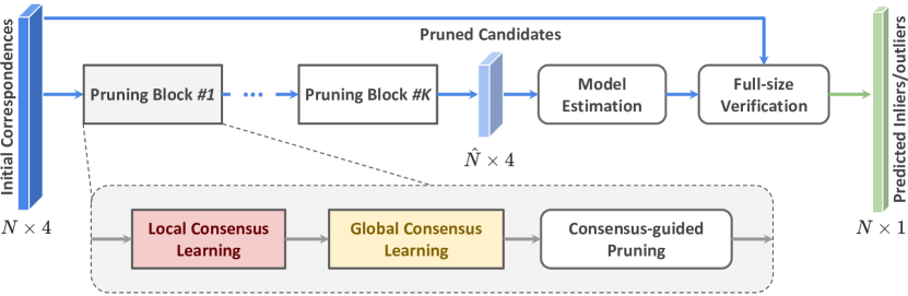
Figure 3: Overall framework. $N$ represents the number of matches and $4$ denotes the 4D locations of matched keypoints. We gradually prune the raw data into $\hat{N}$ candidates via $K$ pruning blocks guided by local-to-global consensus learning. A parametric model is then estimated, employing inliers identified among the $\hat{N}$ candidates. A full-size verification is further conducted based on the estimated model, yielding $N\times 1$ inlier/outlier predictions for the initial correspondences.

3.1 Problem Formulation

Given an image pair $(\mathbf{I},\mathbf{I}{{}^{\prime}})$, putative correspondences ${\bm{C}}$ can be established via nearest neighbor matching between the descriptors of extracted keypoints. Let us denote the correspondences as ${\bm{C}}=[{{\bm{c}}_{1}},\cdots,{\bm{c}}_{N}]\in\mathbb{R}^{N\times 4}$. ${\bm{c}}_{i}=[x_{i},y_{i},x^{\prime}_{i},y^{\prime}_{i}]$ indicates a correspondence between keypoint $(x_{i},y_{i})$ in image $\mathbf{I}$ and keypoint $(x^{\prime}_{i},y^{\prime}_{i})$ in image $\mathbf{I^{\prime}}$. Any off-the-shelf detectors and descriptors can be used for this task, either handcrafted methods [26, 35] or learned ones [28, 11]. In any event, the putative correspondences ${\bm{C}}$ often contain a huge proportion of mismatches, and correspondence pruning thus aims to identify the correct matches (inliers) ${\bm{C}}_{p}$ while rejecting the incorrect ones (outliers) ${\bm{C}}_{n}$.

Existing learning-based methods [29, 40] typically cast the correspondence pruning as an inlier/outlier classification problem, adopting permutation-invariant neural networks to predict inlier weights ${\bm{w}}=\tanh(\text{ReLU}({\bm{o}}))\in[0,1)$ for all putative correspondences ${\bm{C}}$, where ${\bm{o}}$ is the output of network. ${\bm{c}}_{i}\in{\bm{C}}$ is then categorized as an outlier if its predicted weight ${w}_{i}=0$. The predicted weights ${\bm{w}}$ are not only utilized to identify inliers but also as auxiliary input for model estimation, e.g., to compute the essential matrix $\hat{{\bm{E}}}$ for camera pose estimation [15]. In other words, predicting accurate weights ${\bm{w}}$ is at the core of learning-based correspondence pruning methods. This, however, is complicated by the dominant presence of outliers in ${\bm{C}}$. Furthermore, the fact that existing methods [29, 40] do not explicitly model the contextual information across ${\bm{C}}$ makes the pruning process even more difficult.

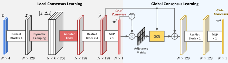
Figure 4: Detailed architecture of the proposed pruning block. A pruning block consists of local-to-global consensus learning layers. Each ResNet block [16] contains two MLPs followed by Context Normalization [29], Batch Normalization [17], and ReLU. Note that Attentive Context Normalization [40] is not used in our method, because it requires additional supervision. We select a subset of candidates from input correspondences according to the estimated global consensus scores.

In this paper, we advocate for progressively pruning ${\bm{C}}$ into a subset of candidates $\hat{{\bm{C}}}$, mitigating the effect of dominant presence of outliers. By predicting inlier weights $\hat{{\bm{w}}}$ for the pruned subset $\hat{{\bm{C}}}$ which is expected to be more reliable than ${\bm{C}}$, inliers $\hat{{\bm{C}}}_{p}$ can be obtained more easily. We then estimate a parametric model (essential matrix $\hat{{\bm{E}}}$ as an example) from $\hat{{\bm{C}}}_{p}$. In turn, this model is adopted to perform a full-size verification on the entire set ${\bm{C}}$. Some inliers falsely rejected by pruning are expected to be recovered after the verification. Our solution therefore follows the “generation-verification” paradigm, as the classical and effective RANSAC algorithm [12].

Formally, our approach can be expressed as

$$\hat{{\bm{C}}}=f_{\phi}({\bm{C}}),~{}~{}~{}~{}(\hat{{\bm{w}}}_{p},\hat{{\bm{C}}}_{p})=f_{\psi}(\hat{{\bm{C}}})$$

$$\hat{{\bm{E}}}=g(\hat{{\bm{w}}}_{p},\hat{{\bm{C}}}_{p}),~{}~{}~{}~{}{\bm{w}}=h(\hat{{\bm{E}}},{\bm{C}}),$$ (1)

where $f_{\phi}$ and $f_{\psi}$ are deep neural networks with learnable parameters $\phi$ and $\psi$ that perform correspondence pruning and inlier identification, respectively; $g(\cdot,\cdot)$ denotes the parametric model estimation (generation) process; the optional $h(\cdot,\cdot)$ performs a full-size verification (prediction).

3.2 Local-to-Global Consensus Learning

To design the network $f_{\phi}()$, we leverage the intuition that inliers should be consistent in both their local and global contexts, and thus propose to estimate consensus scores from local-to-global graphs. Correspondences with high scores are preserved whereas those with low scores are removed as outliers.

As illustrated in Fig. 3, our framework includes a sequence of “pruning” blocks, which progressively prune correspondences, i.e., ${\bm{C}}\to\cdots\to\hat{{\bm{C}}}$. Each block consists of local and global consensus layers, the detail of which is shown in Fig. 4. In what follows, without loss of generality and for ease of notation, we denote the input to a “pruning” block as ${\bm{C}}\in\mathbb{R}^{N\times 4}$ and its output as $\hat{{\bm{C}}}\in{\mathbb{R}}^{\hat{N}\times 4}$, where $\hat{N}<N$. Note, however, that each block truly takes as input the output of the previous block. Let us now define the operations of a pruning block in more detail.

Local consensus.

We propose to leverage local context for each correspondence ${\bm{c}}_{i}$ by building a $k$-nearest neighbor graph denoted as

$${\mathcal{G}}_{i}^{l}=({\mathcal{V}}_{i}^{l},{\mathcal{E}}_{i}^{l}),~{}~{}~{}1\leq i\leq N,$$ (2)

where ${\mathcal{V}}_{i}^{l}=\{{\bm{c}}_{i}^{1},\cdots,{\bm{c}}_{i}^{k}\}$ are $k$-nearest neighbors of ${\bm{c}}_{i}$ in feature space, and ${\mathcal{E}}_{i}^{l}$ indicates the set of directed edges that connect ${\bm{c}}_{i}$ and its neighbors in ${\mathcal{V}}_{i}^{l}$. Specifically, given ${\bm{c}}_{i}\in{\bm{C}}$, we extract a feature representation ${\bm{z}}_{i}$ via a series of ResNet blocks [16]. The $k$-nearest neighbors of ${\bm{c}}_{i}$ are determined by ranking the Euclidean distances between ${\bm{z}}_{i}$ and $\{{\bm{z}}_{j}|1\leq j\leq N,j\neq i\}$. Following [45], we describe the features between ${\bm{c}}_{i}$ and each neighbor as

$${\bm{e}}_{i}^{j}=[{\bm{z}}_{i},\Delta{\bm{z}}_{i}^{j}],~{}~{}~{}1\leq j\leq k$$ (3)

where $[\cdot,\cdot]$ represents the concatenation; $\Delta{\bm{z}}_{i}^{j}={\bm{z}}_{i}-{\bm{z}}_{i}^{j}$ is the residual feature of ${\bm{c}}_{i}$ and the $j$-th neighbor ${\bm{c}}_{i}^{j}$.

Our goal then is to compute a local consensus score from the local graph ${\mathcal{G}}_{i}^{l}$ for ${\bm{c}}_{i}$. Intuitively, we split such a process into two steps: 1) Aggregating the features $\{{\bm{e}}_{i}^{j}|1\leq j\leq k\}\to\tilde{{\bm{z}}}_{i}$ by passing messages along graph edges ${\mathcal{E}}_{i}^{l}$, and 2) predicting a consensus score from $\tilde{{\bm{z}}}_{i}$ via MLPs. A naïve way for feature aggregation consists of using MLPs followed by pooling layers [45]. However, this operation may discard the structural information in the graphs, i.e., the fine-grained relations among graph nodes, because the $1\times 1$ kernels of MLPs extract features from neighbors separately.

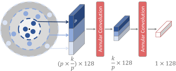
Figure 5: Illustration of the proposed annular convolution. The nodes (colored dots) in a local graph are grouped into annuli based on their affinities to the anchor. The features in each annulus are aggregated by a convolution kernel.

To make the most of the graph knowledge, we therefore introduce an annular convolutional layer which considers both the affinities of neighbors to the anchor and the relative relationships among neighbors in each annulus. Specifically, as shown in Fig. 5, nodes are sorted based on the affinities to the anchor and then assigned into $k/p$ annuli, where $p$ denotes the number of nodes in each annulus and $k$ is expected to be divisible by $p$. We aggregate the features in each annulus via $1\times p$ convolution kernels as

$$\tilde{{\bm{e}}}_{i}^{t}=\sum\mathbf{W}{\bm{e}}_{i}^{j}+\mathbf{b},~{}~{}~{}(t-1)p\leq j\leq tp$$ (4)

where $\tilde{{\bm{e}}}_{i}^{t}$ denotes the aggregated feature of the $t$-th annulus; $\mathbf{W}$ and $\mathbf{b}$ are learnable parameters. $\{\tilde{{\bm{e}}}_{i}^{t}|1\leq t\leq k/p\}$ are further integrated by another annular convolution, i.e., the second one in Fig. 5, with its own set of trainable parameters. These operations are followed by ResNet blocks to extract a feature vector $\tilde{{\bm{z}}}_{i}$, which we further transform into a local consensus score ${w}_{i}^{l}$. ${w}_{i}^{l}$ reflects the consistency of ${\bm{c}}_{i}$ in the local receptive field. In other words, ${w}_{i}^{l}$ roughly measures the inlier weight of ${\bm{c}}_{i}$ when only considering its local context.

Global consensus.

To encode global contextual information, we connect the local graphs into a global one. The global graph is denoted as

$${\mathcal{G}}^{g}=({\mathcal{V}}^{g},{\mathcal{E}}^{g}),$$ (5)

where nodes ${\mathcal{V}}^{g}$ are represented by $\mathbf{C}$ with local aggregated features $\{\tilde{{\bm{z}}}_{1},\cdots,\tilde{{\bm{z}}}_{N}\}$, and edges ${\mathcal{E}}^{g}$ connect every two correspondences $(\mathbf{c}_{i},\mathbf{c}_{j}),1\leq i,j\leq N,i\neq j$. We encode the affinity of $(\mathbf{c}_{i},\mathbf{c}_{j})$ using the local consensus scores as

$$e^{g}_{ij}={w}^{l}_{i}\cdot{w}^{l}_{j},1\leq i,j\leq N.$$ (6)

The product of $({w}^{l}_{i},{w}^{l}_{j})$ enables $e^{g}_{ij}$ to indicate the compatibility of $(\mathbf{c}_{i},\mathbf{c}_{j})$. An adjacency matrix $\mathbf{A}\in\mathbb{R}^{N\times N}$ is then built with $\mathbf{A}_{ij}=e^{g}_{ij}$ to explicitly describe the global context. Specifically, we exploit $\mathbf{A}$ to compute a global embedding

$${\bm{f}}^{g}=\mathbf{L}[\tilde{{\bm{z}}}_{1},\cdots,\tilde{{\bm{z}}}_{N}]\mathbf{W}^{g},$$ (7)

$$\mathbf{L}=\widetilde{\mathbf{D}}^{-\frac{1}{2}}\widetilde{\mathbf{A}}\widetilde{\mathbf{D}}^{-\frac{1}{2}},$$ (8)

where $\{\tilde{{\bm{z}}}\}$ are the aggregated features obtained from local consensus learning; $\mathbf{W}^{g}$ is a learnable matrix; $\mathbf{L}$ is the graph Laplacian [21]; $\widetilde{\mathbf{A}}=\mathbf{A}+\mathbf{I}_{N}$ for numerical stability; $\widetilde{\mathbf{D}}\in\mathbb{R}^{N\times N}$ is the diagonal degree matrix of $\widetilde{\mathbf{A}}$. In short, $\mathbf{L}$ modulates $\{\tilde{{\bm{z}}}\}$ into the spectral domain, considering the isolated local embeddings in a joint manner, and the feature filter $\mathbf{W}^{g}$ in the spectral domain enables the propagated features to reflect the consensus from the global graph Laplacian. Similar to local consensus learning, global consensus scores ${\bm{w}}^{g}$ are estimated by encoding the aggregated features via a ResNet block followed by MLPs.

Consensus-guided pruning.

Since the global consensus scores jointly consider both global and local context, we prune the putative correspondences based on their global consensus scores ${\bm{w}}^{g}$. Specifically, the elements in ${\bm{C}}$ are sorted by a descending value of ${\bm{w}}^{g}$. We preserve the top-$\hat{N}$ correspondences and discard the remaining ones as outliers. The back propagation can be achieved by only keeping the gradients of top-$\hat{N}$ correspondences. Furthermore, inspired by [47], we take local and global consensus scores as additional input to the next pruning block. A ResNet block and MLPs are used after the last pruning block to predict inlier weights $\hat{{\bm{w}}}$ for the pruned candidates.

Training objectives.

Learning-based correspondence pruning methods [29, 40] generally combine an inlier/outlier classification loss and a regression loss as the training objective. For camera pose estimation, on widely-used benchmarks [29, 47, 18], the ground-truth labels ${\bm{s}}$ of ${\bm{C}}$ are assigned using the epipolar distances with an ad-hoc threshold $d_{\text{thr}}$, empirically set to $1e$-$4$ [47].

Although training with a conventional binary cross-entropy loss has achieved satisfactory performance [29, 48, 47], we argue that inevitable label ambiguity exists, especially for the correspondences whose epipolar distances are close to $d_{\text{thr}}$. Typically, the confidence of ${\bm{c}}_{i}$ should be negatively correlated with the corresponding epipolar distance $d_{i}$, i.e. $d_{i}\to 0$ for an inlier. To reflect this intuition, we introduce an adaptive temperature for putative inliers ($d_{i}<d_{\text{thr}}$) to alleviate the effect of label ambiguity, computed as

$$\tau_{i}=\exp({-\frac{\|d_{i}-d_{\text{thr}}\|_{1}}{d_{\text{thr}}}}).$$ (9)

For outliers ${\bm{c}}_{i}$ with $d_{i}>=d_{\text{thr}}$, we set $\tau_{i}=1$.

The overall training objective is then denoted as

$$\mathcal{L}=\mathcal{L}_{\text{cls}}+\lambda\mathcal{L}_{\text{reg}}({\hat{\mathbf{E}},\mathbf{E}}),$$ (10)

where $\mathcal{L}_{\text{cls}}$ is a binary classification loss with our proposed adaptive temperature, $\mathcal{L}_{\text{reg}}$ represents a geometric loss [47] on estimated parametric model $\hat{\mathbf{E}}$, and $\lambda$ is a weighting factor. $\mathcal{L}_{\text{cls}}$ is formulated as

$$\mathcal{L}_{\text{cls}}=\sum_{j=1}^{K}\Big{(}\ell_{\text{bce}} (\sigma(\mathbf{{\bm{\mathsfit{\tau}}}}_{j}\odot\mathbf{o}_{j}^{l}),\mathbf{y}_{j})+\ell_{\text{bce}}(\sigma(\mathbf{{\bm{\mathsfit{\tau}}}}_{j}\odot\mathbf{o}_{j}^{g}),\mathbf{y}_{j})\Big{)}$$

$$+\ell_{\text{bce}}(\sigma(\hat{\mathbf{{\bm{\mathsfit{\tau}}}}}\odot\hat{\mathbf{o}}),\mathbf{y}),$$ (11)

where ${\bm{o}}_{j}^{l}$, ${\bm{o}}_{j}^{g}$ are the outputs of local and global consensus learning layers in $j$-th pruning block, respectively; $\hat{\mathbf{o}}$ is the output of the last MLP in CLNet; $\bf{{\bm{\mathsfit{\tau}}}}$ is a vector of temperatures estimated by Eq. 9; $\sigma$ represents the sigmoid function; $\odot$ indicates the Hadamard product; $\mathbf{y}$ denotes the set of binary ground-truth labels; $\ell_{\text{bce}}$ indicates a binary cross-entropy loss; $K$ is the number of pruning blocks. As a result, an inlier $c_{i}$ with a smaller $d_{i}$ would be more confident to enforce larger regularization on the model optimization via a smaller temperature.

4 Experiments

We conduct experiments on four datasets, covering the tasks of robust line fitting (Section 4.2), camera pose estimation (Section 4.3), and retrieval-based image localization (Section 4.4). In Section 4.5, we provide a comprehensive analysis of our method to demonstrate the effectiveness of its components.

4.1 Implementation Details

In our experiments, we use two sequential pruning blocks, pruning the $N$ putative correspondences into $N/4$ candidates, i.e., pruning by half in each block. We set the number of nearest neighbors used to establish the local graphs to $k=9$ and $k=6$ for the two blocks, respectively. We use $p=3$ for annular convolutions and $\lambda=0.5$ in Eq. (10). $h(\cdot)$ in Eq. (1) is implemented by the epipolar constraint [15] for camera pose estimation and image localization. For training, we use the Adam [20] optimizer with a batch size of 32 and a constant learning rate of $10^{-3}$.

4.2 Robust Line Fitting

As a first experiment, to evaluate robustness to different outlier distributions, we focus on the task of robust line fitting [40]. Note that this task differs from the correspondence selection problem, showing the ability of our method to address general inlier/outlier classification tasks. In this case, the input data to our network consists of 2D points $[x,y]$ instead of 4D correspondences $[x,y,x^{{}^{\prime}},y^{{}^{\prime}}]$. Specifically, we create synthetic data by considering a 2D line $ax+by+c=0$ with parameters $(a,b,c)$ randomly sampled in $[0,1]$. We generate inliers by randomly sampling $x\in[-5,5]$ and estimating $y$ using the line equation. Outliers are obtained via uniformly randomly sampling $(x,y)$ in $[-5,5]$. For each line, we generate $N=1000$ points, from which we seek to identify the inliers. We then compute $(a,b,c)$ using the least-square solution of [23]. $6000$, $2000$, and $2000$ data are used for training, validation, and testing, respectively. In addition to our method, we retrained PointCN [29], OANet [47], and PointACN [40] using the official implementations released by the authors.

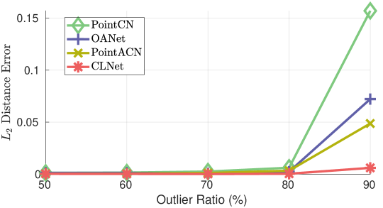
Figure 6: Robust line fitting performance. We report the $L_{2}$ distance between the predicted line parameters and the ground-truth ones for five different outlier ratios, varying from $50\%$ to $90\%$.

Fig. 6 summarizes the results of our line-fitting experiment for an outlier ratio ranging from $50\%$ to $90\%$. We report the $L_{2}$ distance between the ground-truth $(a,b,c)$ and the predicted ones. While all methods perform well for relatively low outlier ratios, ours significantly outperforms the competitors for high ones, i.e. $90\%$ outliers. This evidences the benefits of pruning the input data instead directly trying to classify each input sample.

4.3 Camera Pose Estimation

For camera pose estimation, we exploit the outdoor YFCC100M [43] and indoor SUN3D [46] datasets, following the settings in [47, 36] (more results on ScanNet [10] and the benchmark of [47] can be found in the appendix). Initial matches are generated by nearest neighbor matching with SIFT [26], unless otherwise specified. The keypoint coordinates in ${\bm{C}}$ are normalized using the camera intrinsics, as in [29]. Following [36], we report the AUCs of the pose error at different thresholds ($5^{\circ},10^{\circ},20^{\circ}$).

Method	Desc	YFCC100M [43] (outdoor) (%)
		AUC@$5^{\circ}$	AUC@$10^{\circ}$	AUC@$20^{\circ}$
RANSAC [12]	✓	14.33	27.08	42.27
MAGSAC [3]	✓	17.01	29.49	44.03
LPM [27]	✗	10.22	20.65	33.96
GMS [4]	✗	19.05	32.35	46.79
CODE [24]	✗	16.99	30.23	43.85
PointCN [29]	✗	26.53	43.93	61.01
NM-Net [48]	✗	28.56	46.53	63.55
NG-RANSAC [5]	✓	27.17	43.60	59.63
OANet [47]	✗	28.76	48.42	66.18
PointACN [40]	✗	28.81	48.02	65.39
SuperGlue [36]	✓	30.49	51.29	69.72
Our CLNet	✗	32.79	52.70	69.76

Method	SUN3D [46] (indoor) (%)
	AUC@$5^{\circ}$	AUC@$10^{\circ}$	AUC@$20^{\circ}$
RANSAC [12]	3.93	10.28	21.04
MAGSAC [3]	3.94	10.33	21.25
LPM [27]	3.31	8.56	17.73
GMS [4]	4.36	11.08	21.68
CODE [24]	3.52	8.91	18.32
PointCN [29]	5.86	14.40	27.12
NM-Net [48]	6.45	16.44	31.16
NG-RANSAC [5]	6.65	16.46	30.86
OANet [47]	6.83	17.10	32.28
PointACN [40]	7.10	17.92	33.56
Our CLNet	7.78	19.07	35.25

Table 1: Pose estimation on YFCC100M [43] and SUN3D [46]. “Desc” indicates whether descriptors are required as input. For [12, 3, 5], the ratio test of [26] is employed to prune the correspondences.

Method	AUC@$5^{\circ}$	AUC@$10^{\circ}$	AUC@$20^{\circ}$
PointCN [29]	12.38	28.15	48.04
NM-Net [48]	12.59	30.62	52.07
OANet [47]	16.86	36.74	57.40
PointACN [40]	18.64	38.76	59.56
Our CLNet	26.19	46.33	65.48

Table 2: Pose estimation without a robust estimator on YFCC100M. For these results, we used the weighted 8-point algorithm [29] instead of a robust estimator, e.g., RANSAC, to estimate the essential matrices.

Method	SUN3D [46] (%)	YFCC100M [43] (%)
	SIFT [26]	ORB [35]	DoG-Hard [28]	SP [11]
PointCN [29]	6.00	5.70	31.89	18.12
NM-Net [48]	5.78	5.26	32.70	17.43
OANet++ [47]	5.60	6.35	32.53	17.75
PointACN [47]	5.55	5.56	32.02	17.62
Our CLNet	6.25	7.68	35.10	18.82

Table 3: Generalization ability. All models were trained on YFCC100M [43] with SIFT [26], and tested on SUN3D [46] with SIFT, and on YFCC100M with ORB [35], DoG-HardNet [28], or SuperPoint(SP) [11]. AUC@$5^{\circ}$(%) is reported.

Table 1 provides the quantitative results on YFCC100M and SUN3D. For RANSAC [12], MAGSAC [3], and NGRANSAC [5], we cleaned the initial correspondences using the ratio test of [26] with a threshold of $0.9$, because we observed the results without ratio test to be significantly worse. For the other methods, following [36], we employ RANSAC as a robust estimator when estimating the essential matrices. Our CLNet delivers the best AUCs on both two datasets, even outperforms the most recent SuperGlue which requires descriptors as input (please refer to the appendix for more comparison with SuperGlue).

We further consider the case of estimating the essential matrices without a robust estimator, i.e., without RANSAC. In this case, we use a weighted 8-point algorithm, as suggested in  [29, 47, 40]. As shown in Table 2, our CLNet achieves remarkably superior results, showing that our iterative pruning scheme makes our approach effective even without requiring an additional RANSAC step.

To evaluate generalization ability, we test all learning-based methods on SUN3D with SIFT, and on YFCC100M with ORB [35], DoG-HardNet [28], or SuperPoint [11], employing the models trained on YFCC100M with SIFT. Our choices of ORB, DoG-HardNet and SuperPoint were motivated by their popularity in SLAM [30], demonstrated robustness [18], and joint detector/descriptor learning ability, respectively. As shown in Table 3, CLNet achieves the best performance in all settings, which shows the robustness of our method to different datasets and detector-descriptor combinations.

4.4 Retrieval-based Image Localization

Accurate retrieval is the premise of image localization [37, 42, 6], providing initial locations of query images by identifying nearby reference images with geographical tags [13]. Existing image-based methods [2, 13] take an image as input and learn a global description of the image for retrieval. We introduce to refine the retrieval results using correspondences as re-ranking of the image-based approaches. We study the benchmark of the famous NetVLAD [2] and its follow-up works [13, 19, 25]. Here, we achieve the coarse-to-fine retrieval with the following three steps: 1) Use image-based methods [2, 13] to search for the top-$k$ ($k$ is empirically set to 100) images for each query. We did not use all reference images for re-ranking due to the computational cost. 2) Perform feature matching, with either an existing method [12, 29] or our approach, on each query-retrieved image pair. 3) Re-rank the top-$k$ images using a refined similarity measure defined as $S_{\text{img}}+S_{\text{inl}}$, where $S_{\text{img}}$ represents the original similarity estimated by image-based methods, and $S_{\text{inl}}$ is the number of selected inliers normalized within $[0,1]$. This approach leveraged the fact that image-based methods exploit global description while correspondence-based ones focus on local patterns, making these two kinds of methods complementary. Note that the correspondences can be further used to estimate camera pose of query images [14], but we concentrates on accurate image retrieval in this section.

In our experiments, we use the state-of-the-art SFRS [13] as image-based method and employ RANSAC [12], PointCN [29] or our CLNet as the post-processing technique. Note that PointCN and CLNet were pretrained on YFCC100M [43]. As shown in Table 4, CLNet improves SFRS by a considerable margin of $6.0$ percentage points in terms of Recall@1. The superiority of our method can be also observed by comparing “CLNet-SFRS” with “RANSAC-SFRS” and “PointCN-SFRS”, with our CLNet yielding the best results.

Method	Tokyo 24/7 [44] (%)
	R@1	R@5	R@10
NetVLAD [2]	73.3	82.9	86.0
CRN [19]	75.2	83.8	87.3
SARE [25]	79.7	86.7	90.5
SFRS [13]	85.4	91.1	93.3
RANSAC [12]-SFRS	88.6 (+3.2)	93.0 (+1.9)	93.7 (+0.4)
PointCN [29]-SFRS	89.5 (+4.1)	93.3 (+2.2)	94.3 (+1.0)
Our CLNet-SFRS	91.4 (+6.0)	94.0 (+2.9)	94.3 (+1.0)

Table 4: Evaluation on the image localization dataset Tokyo 24/7 [44]. We report the Recall@1/5/10.

4.5 Ablation Studies

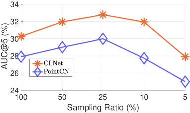
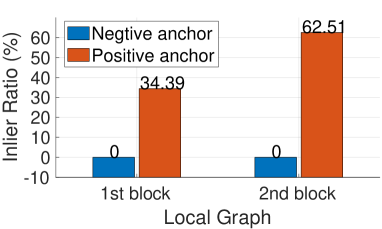
Figure 7: Effectiveness of our consensus-guided pruning. (a) AUC@$5^{\circ}$(%) estimated from candidates sampled by CLNet and PointCN [29] with varying sampling ratios; (b) Inlier ratios of the nodes in the local graphs of CLNet anchored on inliers (positive anchor) and outliers (negative anchor).

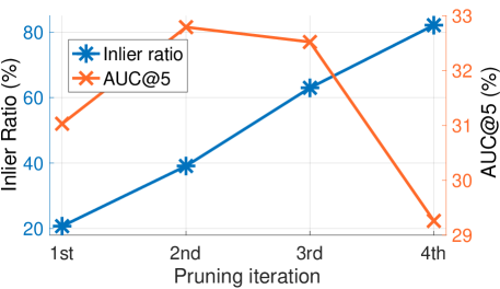
Figure 8: Influence of the number of pruning iterations. We show the inlier ratio of pruned candidates (blue line) and the AUC@$5^{\circ}$(%) (orange line) for different numbers of pruning blocks.

Consensus-guided pruning.

An intuitive solution to acquire candidates from initial data could consist of sampling matches according to the weights predicted by off-the-shelf methods, e.g., PointCN [29]. We therefore evaluate the benefits of our consensus learning strategy over this baseline. Specifically, as baseline, we iteratively perform PointCN twice, which progressively prunes putative correspondences into candidates with a specific sampling ratio; inliers are then identified from the candidates and used to estimate the essential matrix. Fig. 7 compares the baseline to our method with different sampling ratios on YFCC100M. Our CLNet consistently surpasses the baseline by a large margin, which demonstrates the superiority of our consensus-guided pruning strategy. The best AUC of our CLNet is observed with a sampling ratio of $25\%$, i.e., $25\%$ correspondences are sampled as candidates. In Fig. 7 we further explain the effectiveness of our consensus learning by providing inlier ratios of the nodes in the local graphs of our CLNet. The grouped neighbors contain more inliers for graphs anchored on inliers than for graphs anchored on outliers. This demonstrates that our method is capable of enlarging the correspondence consensus in inlier-anchored graphs, while decreasing the correspondence consensus in outlier-anchored ones.

Since we achieve pruning in an iterative fashion, by stacking pruning blocks, we analyze the effect of the number of pruning iterations on candidate consistency and pose estimation accuracy. As shown in Fig. 8, iterative pruning yields an increase of inlier ratio, i.e., from 20% to 80%, which indicates that the candidates are increasingly more consistent as more pruning iterations are performed. The AUC drops after the second iteration, because the number of remaining matches is too small to carry out robust model estimation. Some visual results are shown in Fig. 9. The imbalance of initial matches is alleviated by progressively removing the outliers, making it increasingly easier to identify the inliers.

	Annular Conv.	MLP & Max-pooling
AUC@$5^{\circ}$ (%)	32.79	31.99

Table 5: Comparison between the proposed annular convolution and an mlp-pooling strategy. “MLP & Max-pooling” extracts and aggregates local features with MLPs and max-pooling layers, respectively. We report the AUC@$5^{\circ}$(%) on YFCC100M [43].

Local Cons.	Global Cons.	Adaptive temp.	AUC@$5^{\circ}$ (%)
✗	✗	✗	29.99
✓	✗	✗	30.94
✓	✓	✗	31.70
✓	✓	✓	32.79

Table 6: Influence of the individual components of CLNet. All models were trained and tested on YFCC100M [44].

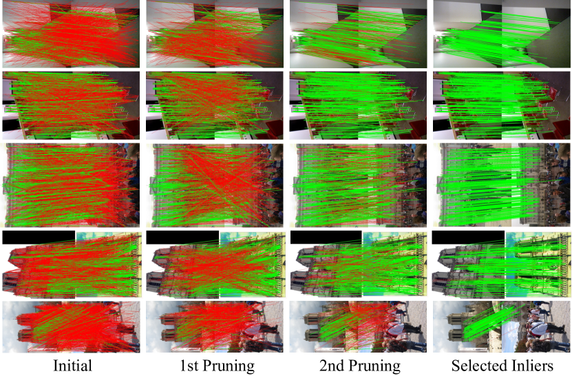
Figure 9: Visualization of progressive pruning. Outliers and inliers are indicated by red lines and green lines, respectively.

To further understand the importance of each component in CLNet, in Table 5, we compare the proposed annular convolution with the mlp-pooling strategy that has been employed in [32, 45]. Our annular convolution yields a $0.80$ percentage point AUC improvement on YFCC100M, demonstrating its effectiveness. Furthermore, we evaluate different combinations of our method’s components in Table 6. As expected, all components contribute to the optimal performance of our approach. In particular, local-to-global consensus learning leads to a $1.71$ percentage point AUC improvement (third row vs. first row), and the performance is further boosted by applying adaptive temperatures. Note that progressive pruning is utilized in all cases.

5 Conclusion

To overcome the negative impact of the dominant outliers, we have proposed to progressively prune the putative correspondences into more reliable candidates with a local-to-global consensus learning network. Our framework builds local and global graphs on-the-fly, which explicitly describe the correspondence consensus in local and global contexts, facilitating pruning. Our experiments in diverse scenarios have demonstrated that the proposed progressive pruning strategy largely alleviates the effect of randomly distributed outliers, showing significant improvements over state-of-the-arts on multiple benchmarks. As the candidates are sampled using a constant ratio in our current framework, we will consider about a pruning strategy with adaptive ratios in our future work.

References

- [1] Andrea Albarelli, Emanuele Rodolà, and Andrea Torsello. Imposing semi-local geometric constraints for accurate correspondences selection in structure from motion: A game-theoretic perspective. Int. J. Comput. Vis., 97(1):36–53, 2012.
- [2] Relja Arandjelovic, Petr Gronat, Akihiko Torii, Tomas Pajdla, and Josef Sivic. Netvlad: Cnn architecture for weakly supervised place recognition. In IEEE Conf. Comput. Vis. Pattern Recog., pages 5297–5307, 2016.
- [3] Daniel Barath, Jiri Matas, and Jana Noskova. Magsac: marginalizing sample consensus. In IEEE Conf. Comput. Vis. Pattern Recog., pages 10197–10205, 2019.
- [4] JiaWang Bian, Wen-Yan Lin, Yasuyuki Matsushita, Sai-Kit Yeung, Tan-Dat Nguyen, and Ming-Ming Cheng. Gms: Grid-based motion statistics for fast, ultra-robust feature correspondence. In IEEE Conf. Comput. Vis. Pattern Recog., pages 4181–4190, 2017.
- [5] Eric Brachmann and Carsten Rother. Neural-guided ransac: Learning where to sample model hypotheses. In Int. Conf. Comput. Vis., pages 4322–4331, 2019.
- [6] Eric Brachmann and Carsten Rother. Visual camera re-localization from rgb and rgb-d images using dsac. arXiv preprint arXiv:2002.12324, 2020.
- [7] Matthew Brown and David G Lowe. Automatic panoramic image stitching using invariant features. Int. J. Comput. Vis., 74(1):59–73, 2007.
- [8] Ondrej Chum and Jiri Matas. Matching with prosac-progressive sample consensus. In IEEE Conf. Comput. Vis. Pattern Recog., volume 1, pages 220–226. IEEE, 2005.
- [9] Ondřej Chum, Jiří Matas, and Josef Kittler. Locally optimized ransac. In Joint Pattern Recognition Symposium, pages 236–243. Springer, 2003.
- [10] Angela Dai, Angel X Chang, Manolis Savva, Maciej Halber, Thomas Funkhouser, and Matthias Nießner. Scannet: Richly-annotated 3d reconstructions of indoor scenes. In IEEE Conf. Comput. Vis. Pattern Recog., pages 5828–5839, 2017.
- [11] Daniel DeTone, Tomasz Malisiewicz, and Andrew Rabinovich. Superpoint: Self-supervised interest point detection and description. In IEEE Conf. Comput. Vis. Pattern Recog. Worksh., pages 224–236, 2018.
- [12] Martin A Fischler and Robert C Bolles. Random sample consensus: a paradigm for model fitting with applications to image analysis and automated cartography. Communications of the ACM, 24(6):381–395, 1981.
- [13] Yixiao Ge, Haibo Wang, Feng Zhu, Rui Zhao, and Hongsheng Li. Self-supervising fine-grained region similarities for large-scale image localization. In Eur. Conf. Comput. Vis., 2020.
- [14] Hugo Germain, Guillaume Bourmaud, and Vincent Lepetit. S2dnet: Learning accurate correspondences for sparse-to-dense feature matching. arXiv preprint arXiv:2004.01673, 2020.
- [15] Richard Hartley and Andrew Zisserman. Multiple view geometry in computer vision. Cambridge university press, 2003.
- [16] Kaiming He, Xiangyu Zhang, Shaoqing Ren, and Jian Sun. Deep residual learning for image recognition. In IEEE Conf. Comput. Vis. Pattern Recog., pages 770–778, 2016.
- [17] Sergey Ioffe and Christian Szegedy. Batch normalization: Accelerating deep network training by reducing internal covariate shift. arXiv preprint arXiv:1502.03167, 2015.
- [18] Yuhe Jin, Dmytro Mishkin, Anastasiia Mishchuk, Jiri Matas, Pascal Fua, Kwang Moo Yi, and Eduard Trulls. Image matching across wide baselines: From paper to practice. arXiv preprint arXiv:2003.01587, 2020.
- [19] Hyo Jin Kim, Enrique Dunn, and Jan-Michael Frahm. Learned contextual feature reweighting for image geo-localization. In IEEE Conf. Comput. Vis. Pattern Recog., pages 3251–3260. IEEE, 2017.
- [20] Diederik P Kingma and Jimmy Ba. Adam: A method for stochastic optimization. arXiv preprint arXiv:1412.6980, 2014.
- [21] Thomas N Kipf and Max Welling. Semi-supervised classification with graph convolutional networks. arXiv preprint arXiv:1609.02907, 2016.
- [22] Alex Krizhevsky, Ilya Sutskever, and Geoffrey E Hinton. Imagenet classification with deep convolutional neural networks. Communications of the ACM, 60(6):84–90, 2017.
- [23] Charles L Lawson and Richard J Hanson. Solving least squares problems. SIAM, 1995.
- [24] Wen-Yan Lin, Fan Wang, Ming-Ming Cheng, Sai-Kit Yeung, Philip HS Torr, Minh N Do, and Jiangbo Lu. Code: Coherence based decision boundaries for feature correspondence. IEEE Trans. Pattern Anal. Mach. Intell., 40(1):34–47, 2017.
- [25] Liu Liu, Hongdong Li, and Yuchao Dai. Stochastic attraction-repulsion embedding for large scale image localization. In IEEE Conf. Comput. Vis. Pattern Recog., pages 2570–2579, 2019.
- [26] David G Lowe. Distinctive image features from scale-invariant keypoints. Int. J. Comput. Vis., 60(2):91–110, 2004.
- [27] Jiayi Ma, Ji Zhao, Junjun Jiang, Huabing Zhou, and Xiaojie Guo. Locality preserving matching. Int. J. Comput. Vis., 127(5):512–531, 2019.
- [28] Anastasiia Mishchuk, Dmytro Mishkin, Filip Radenovic, and Jiri Matas. Working hard to know your neighbor’s margins: Local descriptor learning loss. In Adv. Neural Inform. Process. Syst., pages 4826–4837, 2017.
- [29] Kwang Moo Yi, Eduard Trulls, Yuki Ono, Vincent Lepetit, Mathieu Salzmann, and Pascal Fua. Learning to find good correspondences. In IEEE Conf. Comput. Vis. Pattern Recog., pages 2666–2674, 2018.
- [30] Raul Mur-Artal, Jose Maria Martinez Montiel, and Juan D Tardos. Orb-slam: a versatile and accurate monocular slam system. IEEE Transactions on Robotics, 31(5):1147–1163, 2015.
- [31] James Philbin, Michael Isard, Josef Sivic, and Andrew Zisserman. Descriptor learning for efficient retrieval. In Eur. Conf. Comput. Vis., pages 677–691. Springer, 2010.
- [32] Charles Ruizhongtai Qi, Li Yi, Hao Su, and Leonidas J Guibas. Pointnet++: Deep hierarchical feature learning on point sets in a metric space. In Adv. Neural Inform. Process. Syst., pages 5099–5108, 2017.
- [33] Rahul Raguram, Ondrej Chum, Marc Pollefeys, Jiri Matas, and Jan-Michael Frahm. Usac: a universal framework for random sample consensus. IEEE Trans. Pattern Anal. Mach. Intell., 35(8):2022–2038, 2012.
- [34] Shaoqing Ren, Kaiming He, Ross Girshick, and Jian Sun. Faster r-cnn: Towards real-time object detection with region proposal networks. In Adv. Neural Inform. Process. Syst., pages 91–99, 2015.
- [35] Ethan Rublee, Vincent Rabaud, Kurt Konolige, and Gary Bradski. Orb: An efficient alternative to sift or surf. In Int. Conf. Comput. Vis., pages 2564–2571. Ieee, 2011.
- [36] Paul-Edouard Sarlin, Daniel DeTone, Tomasz Malisiewicz, and Andrew Rabinovich. Superglue: Learning feature matching with graph neural networks. In IEEE Conf. Comput. Vis. Pattern Recog., pages 4938–4947, 2020.
- [37] Torsten Sattler, Michal Havlena, Konrad Schindler, and Marc Pollefeys. Large-scale location recognition and the geometric burstiness problem. In IEEE Conf. Comput. Vis. Pattern Recog., pages 1582–1590, 2016.
- [38] Kristy Sim and Richard Hartley. Removing outliers using the linfty norm. In IEEE Conf. Comput. Vis. Pattern Recog., volume 1, pages 485–494. IEEE, 2006.
- [39] Noah Snavely, Steven M Seitz, and Richard Szeliski. Modeling the world from internet photo collections. Int. J. Comput. Vis., 80(2):189–210, 2008.
- [40] Weiwei Sun, Wei Jiang, Eduard Trulls, Andrea Tagliasacchi, and Kwang Moo Yi. Acne: Attentive context normalization for robust permutation-equivariant learning. In IEEE Conf. Comput. Vis. Pattern Recog., pages 11286–11295, 2020.
- [41] Richard Szeliski. Image mosaicing for tele-reality applications. In Proceedings of 1994 IEEE Workshop on Applications of Computer Vision, pages 44–53. IEEE, 1994.
- [42] Hajime Taira, Masatoshi Okutomi, Torsten Sattler, Mircea Cimpoi, Marc Pollefeys, Josef Sivic, Tomas Pajdla, and Akihiko Torii. Inloc: Indoor visual localization with dense matching and view synthesis. In IEEE Conf. Comput. Vis. Pattern Recog., pages 7199–7209, 2018.
- [43] Bart Thomee, David A Shamma, Gerald Friedland, Benjamin Elizalde, Karl Ni, Douglas Poland, Damian Borth, and Li-Jia Li. Yfcc100m: The new data in multimedia research. Communications of the ACM, 59(2):64–73, 2016.
- [44] Akihiko Torii, Relja Arandjelovic, Josef Sivic, Masatoshi Okutomi, and Tomas Pajdla. 24/7 place recognition by view synthesis. In IEEE Conf. Comput. Vis. Pattern Recog., pages 1808–1817, 2015.
- [45] Yue Wang, Yongbin Sun, Ziwei Liu, Sanjay E Sarma, Michael M Bronstein, and Justin M Solomon. Dynamic graph cnn for learning on point clouds. ACM Trans. Graph., 38(5):1–12, 2019.
- [46] Jianxiong Xiao, Andrew Owens, and Antonio Torralba. Sun3d: A database of big spaces reconstructed using sfm and object labels. In IEEE Conf. Comput. Vis. Pattern Recog., pages 1625–1632, 2013.
- [47] Jiahui Zhang, Dawei Sun, Zixin Luo, Anbang Yao, Lei Zhou, Tianwei Shen, Yurong Chen, Long Quan, and Hongen Liao. Learning two-view correspondences and geometry using order-aware network. In Int. Conf. Comput. Vis., pages 5845–5854, 2019.
- [48] Chen Zhao, Zhiguo Cao, Chi Li, Xin Li, and Jiaqi Yang. Nm-net: Mining reliable neighbors for robust feature correspondences. In IEEE Conf. Comput. Vis. Pattern Recog., pages 215–224, 2019.
- [49] Chen Zhao, Zhiguo Cao, Jiaqi Yang, Ke Xian, and Xin Li. Image feature correspondence selection: A comparative study and a new contribution. IEEE Trans. Image Process., 29:3506–3519, 2020.