Style Normalization and Restitution for Domain Generalization and Adaptation

Abstract

For many practical computer vision applications, the learned models usually have high performance on the datasets used for training but suffer from significant performance degradation when deployed in new environments, where there are usually style differences between the training images and the testing images. For high-level vision tasks, an effective domain generalizable model is expected to be able to learn feature representations that are both generalizable and discriminative. In this paper, we design a novel Style Normalization and Restitution module (SNR) to simultaneously ensure both high generalization and discrimination capability of the networks. In the SNR module, particularly, we filter out the style variations (e.g. , illumination, color contrast) by performing Instance Normalization (IN) to obtain style normalized features, where the discrepancy among different samples and domains is reduced. However, such a process is task-ignorant and inevitably removes some task-relevant discriminative information, which could hurt the performance. To remedy this, we propose to distill task-relevant discriminative features from the residual (i.e., the difference between the original feature and the style normalized feature) and add them back to the network to ensure high discrimination. Moreover, for better disentanglement, we enforce a dual restitution loss constraint in the restitution step to encourage the better separation of task-relevant and task-irrelevant features. We validate the effectiveness of our SNR on different computer vision tasks, including classification, semantic segmentation, and object detection. Experiments demonstrate that our SNR module is capable of improving the performance of networks for domain generalization (DG) and unsupervised domain adaptation (UDA) on many tasks.

I Introduction

Deep neural networks (DNNs) have advanced the state-of-the-arts for a wide variety of computer vision tasks. The trained models typically perform well on the test/validation dataset which follows similar characteristics/distribution as the training data, but suffer from significant performance degradation (poor generalization capability) on unseen datasets that may present different styles [1, 2, 3]. This is ubiquitous in practical applications. For example, we may want to deploy a trained classification or detection model in unseen environments, like a newly opened retail store, or a house. The captured images in the new environments in general present style discrepancy with respect to the training data, such as illumination, color contrast/saturation, quality, etc.  (as shown in Fig. 1). These result in domain gap/shift between the training and testing.

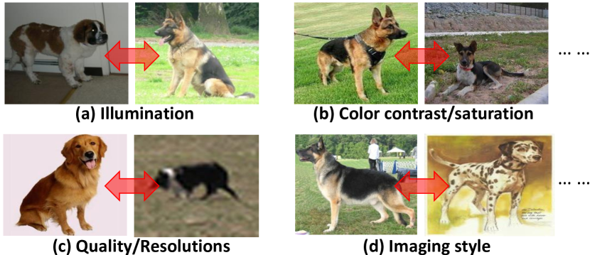
Figure 1: Due to the differences in environments (such as lighting/camera/place/weather), the captured images present style discrepancy, such as the illumination, color contrast/saturation, quality, imaging style. These result in domain gaps between the training and testing data.

To address such domain gap/shift problems, many investigations have been conducted and they could be divided into two categories: domain generalization (DG) [4, 5, 6, 7, 8, 9] and unsupervised domain adaptation (UDA) [10, 11, 12, 2, 13, 14, 15, 16, 17]. DG and UDA both aim to bridge the gaps between source and target domains. DG exploits only labeled source domain data while UDA can also access/exploit the unlabeled data of the target domain for training/fine-tuning. Both do not require the costly labeling on the data of target domain, which is desirable in practical applications.

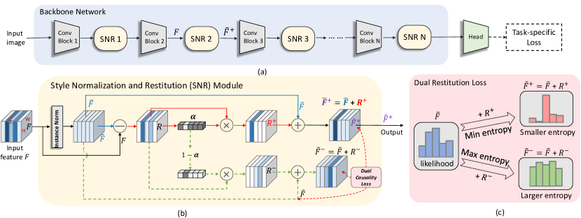
Figure 2: Overall flowchart. (a) Our generalizable feature learning network with the proposed Style Normalization and Restitution (SNR) module being plugged in after some convolutional blocks. Here, we use ResNet-50 as our backbone for illustration. (b) Proposed SNR module. Instance Normalization (IN) is used to eliminate some style discrepancies followed by task-relevant feature restitution (marked by red solid arrows). Note the branch with dashed green line is only used for enforcing loss constraint and is discarded in inference. (c) Dual restitution loss constraint encourages the disentanglement of a residual feature $R$ to task-relevant one ($R^{+}$) and task-irrelevant one ($R^{-}$), which decreases and enhances, respectively, the entropy by adding them to the style normalized feature $\widetilde{F}$ (see Section III-A).

In particular, due to the domain gaps, directly applying a model trained on a source dataset to an unseen target dataset typically suffers from a large performance degradation [4, 5, 6, 7, 8, 9]. As a consequence, feature regularization based UDA methods have been widely investigated to mitigate the domain gap by aligning the domains for better transferring source knowledge to the target domain. Several methods align the statistics, such as the second order correlation [18, 19, 20], or both mean and variance (moment matching) [21, 15], in the networks to reduce the domain discrepancy on features [22, 23]. Some other methods introduce adversarial learning which learns domain-invariant features to deceive domain classifiers [11, 24, 25]. The alignment of domains reduces domain-specific variations but inevitably leads to loss of some discriminative information [26]. Even though many works investigate UDA, the study on domain generalization (DG) is not as extensive.

Domain generalization (DG) aims to design models that are generalizable to previously unseen domains [4, 27, 28, 6, 29, 30], without accessing the target domain data. Classic DG approaches tend to learn domain-invariant features by minimizing the dissimilarity in features across domains [4, 28]. Some other DG methods explore optimization strategies to help improve generalization, e.g., through meta-learning [7], episodic training [9], and adaptive ensemble learning [31]. Recently, Jia et al. [29] and Zhou et al. [32] integrate a simple but effective style regularization operation, i.e., Instance Normalization (IN), in the networks to alleviate the domain discrepancy by reducing appearance style variations, which achieves clear improvement. However, the feature style regularization using IN is task-ignorant and will inevitably remove some task-relevant discriminative information [33, 34], and thus hindering the achievement of high performance.

In this paper, we propose a Style Normalization and Restitution (SNR) method to enhance both the generalization and discrimination capabilities of the networks for computer vision tasks. Fig.  2 shows our proposed SNR module and illustrates the dual restitution loss . We propose to first perform style normalization by introducing Instance Normalization (IN) to our neural network architecture to eliminate style variations. For a feature map of an image, IN normalizes the features across spatial positions on each channel, which reserves the spatial structure but reduces instance-specific style like contrast, illumination [35, 36, 33]. IN reduces style discrepancy among instances and domains, but it inevitably results in the loss of some discriminative information. To remedy this, we propose to distill the task-specific information from the residues (i.e., the difference between the original features and the instance-normalized features) and add it back to the network. Moreover, to better disentangle the task-relevant features from the residual, a dual restitution loss constraint is designed by ensuring the features after restitution of the task-relevant features to be more discriminative than that before restitution, and the features after restitution of task-irrelevant features to be less discriminative than that before restitution.

We summarize our main contributions as follows:

• We propose a Style Normalization and Restitution (SNR) module, a simple yet effective plug-and-play tool, for existing neural networks to enhance their generalization capabilities. To compensate for the loss of discriminative information caused by style normalization, we propose to distill the task-relevant discriminative information from the residual (i.e., the difference between the original feature and the instance-normalized feature).

• We introduce a dual restitution loss constraint in SNR to encourage the better disentanglement of task-relevant features from the residual information.

• The proposed SNR module is generic and can be applied to various networks for different vision tasks to enhance the generalization capability, including object classification, detection, semantic segmentation, etc.. Moreover, thanks to the enhancement of generalization and discrimination capability of the networks, SNR could also improve the performance of the existing UDA networks.

Extensive experiments demonstrate that our SNR significantly improves the generalization capability of the networks and brings improvement to the existing unsupervised domain adaptation networks. This work is an extension of our conference paper [37] which is specifically designed for person re-identification. In this work, we make the design generic and incorporate it into popular generic tasks, such as object classification, detection, semantic segmentation, etc. In addition, we tailor the dual restitution loss to these tasks by leveraging entropy comparisons.

II Related Work

II-A Domain Generalization (DG)

DG considers a challenging setting where the target data is unavailable during training. Some recent DG methods explore optimization strategies to improve generalization, e.g., through meta-learning [7], episodic training [9], or adaptive ensemble learning [31]. Li et al.  [7] propose a meta-learning solution, which uses a model agnostic training procedure to simulate train/test domain shift during training and jointly optimize the simulated training and testing domains within each mini-batch. Episodic training is proposed in  [9], which decomposes a deep network into feature extractor and classifier components, and then train each component by simulating it interacting with a partner who is badly tuned for the current domain. This makes both components more robust. Zhou et al.  [31] propose domain adaptive ensemble learning (DAEL) which learns multiple experts (for different domains) collaboratively so that when forming an ensemble, they can leverage complementary information from each other to be more effective for an unseen target domain. Some other methods augment the samples to enhance the generalization capability [6, 38].

Some DG approaches tend to learn domain-invariant features by aligning the domains/minimizing the feature dissimilarity across domains [4, 28]. Recently, several works attempt to add Instance normalisation (IN) to CNNs to improve the model generalisation ability [34, 29]. Instance normalisation (IN) layers [39] could eliminate instance-specific style discrepancy [40] and IN has been extensively investigated in the field of image style transfer [35, 36, 33], where the mean and variance of IN reflect the style of images. For DG, IN alleviates the style discrepancy among domains/instances, and thus improves the domain generalization [40, 34]. In [34], a CNN called IBN-Net is designed by inserting IN into the shallow layers for enhancing the generalization capability. However, instance normalization is task-ignorant and inevitably introduces the loss of discriminative information [33, 34], leading to inferior performance. Pan et al. [34] use IN and Batch Normalization (BN) together (half of channels use IN while the other half of channels use BN) in the same layer to preserve some discrimination. Nam et al. [41] determine the use of BN and IN (at dataset-level) for each channel based on learned gate parameters. It lacks the adaptivity to instances. Besides, the selection of IN or BN for a channel is hard (0 or 1) rather than soft. In this paper, we propose a style normalization and restitution module. First, we perform IN for all channels to enhance generalization. To assure high discrimination, we go a step further to consider a restitution step, which adaptively distills task-specific features from the residual (removed information) and restitute it to the network.

II-B Unsupervised Domain Adaptation (UDA)

Unsupervised domain adaptation (UDA) belongs to a target domain annotation-free transfer learning task, where the labeled source domain data and unlabeled target domain data are available for training. Existing UDA methods typically explore to learn domain-invariant features by reducing the distribution discrepancy between the learned features of source and target domains. Some methods minimize distribution divergence by optimizing the maximum mean discrepancy (MMD) [12, 2, 23, 42], second order correlation [18, 19, 20], etc. Some other methods learn to achieve domain confusion by leveraging the adversarial learning to reduce the difference between the training and testing domain distributions [11, 25, 43, 44]. Moreover, some recent works tend to separate the model into feature extractor and classifier, and develop some new metric to pull close the learned source and target feature representations. In particular, Maximum Classifier Discrepancy (MCD) [13] maximizes the discrepancy between two classifiers while minimizing it with respect to the feature extractor. Similarly, Minimax Entropy (MME) [45] maximizes the conditional entropy on unlabeled target data w.r.t the classifier and minimizes it w.r.t the feature encoder. M3SDA [15] minimizes the moment distance among the source and target domains and per-domain classifier is used and optimized as in MCD to enhance the alignment.

Our proposed SNR module aims at enhancing the generalization ability and preserving the discrimination capability and thus enhance the existing UDA approaches.

II-C Feature Disentanglement

Learning disentangled representations can help remove irrelevant features [46]. Liu et al. introduce a unified feature disentanglement framework to learn domain-invariant features from data across different domains [47]. Lee et al. propose to disentangle the features into a domain-invariant content space and a domain-specific attributes space, producing diverse outputs without paired training data [48]. Inspired by these works, we propose to disentangle the task-specific features from the discarded/removed residual features, in order to distill and restore the discriminative information. To encourage a better disentanglement, we introduce a dual restitution loss constraint, which enforces a higher discrimination of the feature after the restitution than before. The basic idea is to make the class-likelihood after the restitution to be sharper than before, which enables less ambiguity of a sample.

III Style Normalization and Restitution

We propose a style normalization and restitution (SNR) module which enhances the generalization capability while preserving the discriminative power of the networks for effective DG and DA. Fig. 2 shows the overall flowchart of our framework. Particularly, SNR can be used as a plug-and-play module for existing (e.g., classification/detection/segmentation) networks. Taking the widely used ResNet-50 [49] network as an example (see Fig. 2(a)), SNR module is added after each convolutional block.

In the SNR module (see Fig. 2(b)), we denote the input feature map by $F\in\mathbb{R}^{h\times w\times c}$ and the output by $\widetilde{F}^{+}\in\mathbb{R}^{h\times w\times c}$, where $h,w,c$ denote the height, width, and number of channels, respectively. We first eliminate style discrepancy among samples/instances by performing Instance Normalization (IN). Then, we propose a dedicated restitution step to distill task-relevant (discriminative) feature from the residual (previously discarded by IN, which is the difference between the original feature $F$ and the style normalized feature $\tilde{F}$), and add it to the normalized feature $\tilde{F}$. Moreover, we introduce a dual restitution loss constraint to facilitate the better separation of task-relevant and -irrelevant features within the SNR module (see Fig. 2(c)).

SNR is generic and can be used in different networks for different tasks. We also present the usages of SNR (with small variations on the dual restitution loss forms with respect to different tasks) in detail for different tasks (i.e., object classification, detection, and semantic segmentation). Besides, since SNR can enhance the generalization and discrimination capability of networks which is also very important for UDA, SNR is capable of benefiting the existing UDA networks.

III-A Style Normalization and Restitution Module

III-A1 Style Normalization to Reduce Domain Discrepancy

Real-world images could be captured by different cameras under different scenes and environments (e.g., lighting/camera/place/weather). As shown in Figure 1, the captured images present large style discrepancies (e.g., in illumination, color contrast/saturation, quality, imaging style), especially for samples from two different datasets/domains. Domain discrepancy between the source and target domain generally hinders the generalization capability of learned models.

A learning-theoretic analysis in [4] shows that reducing feature dissimilarity improves the generalization ability on new domains. As discussed in Section II-A, Instance Normalization (IN) actually performs some kinds of style normalization which reduces the discrepancy/dissimilarity among instances/samples [33, 34], so it has the power to enhance the generalization ability of networks [34, 29, 32].

Inspired by that, in SNR module, we first try to reduce the instance discrepancy on the input feature by performing Instance Normalization [39, 36, 35, 33] as

$$\widetilde{F}={\rm{IN}}(F)=\gamma(\frac{F-\mu(F)}{\sigma(F)})+\beta,$$ (1)

where $\mu(\cdot)$ and $\sigma(\cdot)$ denote the mean and standard deviation computed across spatial dimensions independently for each channel and each sample/instance, $\gamma$, $\beta$ $\in\mathbb{R}^{c}$ are parameters learned from the data. IN could filter out some instance-specific style information from the content. With IN performed in the feature space, Huang et al. have argued and experimentally shown that IN has more profound impacts than a simple contrast normalization and it performs a form of style normalization by normalizing feature statistics [33].

However, IN inevitably removes some discriminative information and results in weaker discrimination capability [34]. To address this problem, we propose to distill and restitute the task-specific discriminative feature from the IN removed information, by disentangling it into task-relevant feature and task-irrelevant feature with a dual restitution loss constraint (see Fig. 2(b)). We elaborate on such restitution hereafter.

III-A2 Feature Restitution to Preserve Discrimination

As illustrated in Fig. 2(b), to ensure high discrimination of the features, we propose to restitute the task-relevant feature to the network by distilling it from the residual feature $R$,

$$R=F-\widetilde{F},$$ (2)

which denotes the difference between the original input feature $F$ and the style normalized feature $\widetilde{F}$.

We disentangle the residual feature $R$ in a content adaptive way through channel attention. This is crucial for learning generalizable feature representations since the discriminative components of different images are typically different. Specifically, given $R$, we disentangle it into two parts: task-relevant feature $R^{+}\in\mathbb{R}^{h\times w\times c}$ and task-irrelevant feature $R^{-}\in\mathbb{R}^{h\times w\times c}$, through masking $R$ by a learned channel attention response vector $\textbf{$\mathbf{a}$}=[a_{1},a_{2},\cdots,a_{c}]\in\mathbb{R}^{c}$:

$$R^{+}(:,:,k)= a_{k}R(:,:,k),$$ (3)

$$R^{-}(:,:,k)= (1-a_{k})R(:,:,k),$$

where $R(:,:,k)\in\mathbb{R}^{h\times w}$ denotes the $k^{th}$ channel of feature map $R$, $k=1,2,\cdots,c$. We expect the SE-like [50] channel attention response vector $\mathbf{a}$ to help adaptively distill the task-relevant feature for the restitution,

$$\textbf{$\mathbf{a}$}=g(R)=\sigma({\rm W_{2}}\delta({\rm W_{1}}pool(R))),$$ (4)

where the attention module is implemented by a spatial global average pooling layer, followed by two FC layers (that are parameterized by ${{\rm W_{2}}}\in\mathbb{R}^{(c/r)\times c}$ and ${{\rm W_{1}}}\in\mathbb{R}^{c\times(c/r)}$), $\delta(\cdot)$ and $\sigma(\cdot)$ denote ReLU activation function and sigmoid activation function, respectively. To reduce the number of parameters, a dimension reduction ratio $r$ is set to 16.

By adding this distilled task-relevant feature $R^{+}$ to the style normalized feature $\widetilde{F}$, we obtain the output feature $\widetilde{F}^{+}$ as

$$\widetilde{F}^{+}=\widetilde{F}+R^{+}.$$ (5)

Similarly, by adding the task-irrelevant feature $R^{-}$ to the style normalized feature $\widetilde{F}$, we obtain the contaminated feature $\widetilde{F}^{-}=\widetilde{F}+R^{-}$, which is used in the next loss optimization.

It is worth pointing out that, instead of using two independent attention modules to obtain $R^{+}$, $R^{-}$, respectively, we use $\textbf{$\mathbf{a}$}(\cdot)$, and $1-\textbf{$\mathbf{a}$}(\cdot)$ to facilitate the disentanglement. We will discuss the effectiveness of this operation in the experiment section.

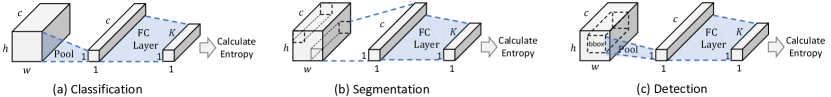
Figure 3: Illustration of obtaining feature vector for restitution loss optimization with respect to different tasks. (a) For classification task, spatial average pooling is performed over the entire feature map ($h\times w\times c)$ to obtain a feature vector of $c$ dimensions (see Section III-B1). (b) For segmentation task (pixel level classification), entropy is calculated for each pixel (see Section III-B2). (c) For detection task (region level classification), spatial average pooling is performed over each groundtruth bounding box (bbox) region to obtain a feature vector of $c$ dimensions (see Section III-B3).

We use the channel attention vector $\mathbf{a}$ to adaptively distill the task-relevant features for restitution for two reasons. (a) Those style factors (e.g., illumination, hue, contrast, saturation) are in general regarded as spatial consistent. We leverage channel attention to select the discriminative style factors distributed in different channels. (b) In our SNR, “disentanglement" aims at better “restitution" of the lost discriminative information due to Instance Normalization (IN). IN reduces style discrepancy of input features by performing normalization across spatial dimensions independently for each channel, where the normalization parameters are the same across different spatial positions. Consistent with IN, we disentangle the features and restitute the task-relevant ones to the normalized features on the channel level.

III-A3 Dual Restitution Loss Constraint

To promote the disentanglement of task-relevant feature and task-irrelevant feature, we design a dual restitution loss constraint by comparing the discrimination capability of features before and after the restitution. The dual restitution loss $\mathcal{L}_{snr}$ consists of $\mathcal{L}_{SNR}^{+}$ and $\mathcal{L}_{SNR}^{-}$, i.e., $\mathcal{L}_{SNR}=\mathcal{L}_{SNR}^{+}+\mathcal{L}_{SNR}^{-}$. As illustrated in Figure 2(c), the physical meaning of the proposed dual restitution loss constraint $\mathcal{L}_{SNR}$ is that: after adding the task-relevant feature $R^{+}$ to the normalized feature $\widetilde{F}$, the enhanced feature becomes more discriminative and its predicted class likelihood becomes less ambiguous (less uncertain) with a smaller entropy; on the other hand, after adding the task-irrelevant feature $R^{-}$ to the normalized feature $\widetilde{F}$, the contaminated feature should become less discriminative, resulting in a larger entropy of the predicted class likelihood.

Taking classification task as an example, we pass the spatially average pooled enhanced feature vector $\mathbf{\widetilde{f}^{+}}=pool(\widetilde{F}+R^{+})\in\mathbb{R}^{c}$ into a FC layer (of $K$ nodes, where $K$ denotes the number of classes) followed by softmax function (we denote these as $\phi(\mathbf{\widetilde{f}^{+}})\in\mathbb{R}^{K}$) and thus obtain its entropy. We denote an entropy function as $H(\cdot)=-p(\cdot)\log p(\cdot)$. Similarly, the contaminated feature vector can be obtained by $\mathbf{\widetilde{f}^{-}}=pool(\widetilde{F}+R^{-})$, and the style normalized feature vector is $\mathbf{\widetilde{f}}=pool(\widetilde{F})$. $\mathcal{L}_{SNR}^{+}$ and $\mathcal{L}_{SNR}^{-}$ are defined as:

$$\mathcal{L}_{SNR}^{+} =Softplus(H(\phi(\mathbf{\widetilde{f}^{+}}))-H(\phi(\mathbf{\widetilde{f}}))),$$ (6)

$$\mathcal{L}_{SNR}^{-} =Softplus(H(\phi(\mathbf{\widetilde{f}}))-H(\phi(\mathbf{\widetilde{f}^{-}}))),$$ (7)

where $Softplus(\cdot)=ln(1+exp(\cdot))$ is a monotonically increasing function that aims to reduce the optimization difficulty by avoiding negative loss values. Intuitively, $\mathcal{L}_{SNR}$ promotes better feature disentanglement of the residual $R$ for feature compensation/restitution. In Eq. (6), the loss encourages higher discrimination after restitution of the task-relevant feature by comparing the discrimination capability of features before and after the restitution. In Eq. (7), the loss encourages lower discrimination capability after restitution of the task-irrelevant feature in comparison with that before the restitution. For other tasks, e.g., segmentation, detection, there are some slight differences, e.g., in obtaining the feature vectors, which are described in the next subsection.

III-B Applications, Extensions, and Variants

The proposed SNR is general. It can improve the generalization and discrimination capability of networks for DG and DA. As a plug-and-play module, SNR can be easily applied into different neural networks for different computer vision tasks, e.g., object classification, segmentation, and detection.

As we described in Section III-A3, we pass the spatially average pooled enhanced/contaminated feature vector $\mathbf{\widetilde{f}^{+}}/\mathbf{\widetilde{f}^{-}}$ into the function $H(\phi(\cdot))$ for obtaining entropy. For the different tasks of classification (i.e., image-level classification), segmentation (i.e., pixel level classification), detection (i.e., region level classification), there are some differences in obtaining the feature vectors for calculating restitution loss. Fig. 3 illustrates the manners to obtain the feature vectors, respectively. We elaborate on them in the following subsections.

III-B1 Classification

For a $K$-category classification task, we take the backbone network of ResNet-50 as an example for describing the usage of SNR. As illustrated in Fig. 2(a), we could insert the proposed SNR module after each convolution block. For a SNR module, given an input feature $F$, we obtain three features–style normalized feature $\widetilde{F}$, enhanced feature $\widetilde{F}^{+}$, and contaminated feature $\widetilde{F}^{-}$. As shown in Fig. 3(a), we spatially averagely pool the features to get the corresponding feature vectors (i.e., $\mathbf{\widetilde{f}}$, $\mathbf{\widetilde{f}^{+}}$, and $\mathbf{\widetilde{f}^{-}}$) to calculate the dual restitution loss for optimization.

III-B2 Segmentation

Semantic segmentation predicts the label for each pixel, which is a pixel wise classification problem. Similar to classification, we insert the SNR modules to the backbone networks of segmentation. Differently, in our restitution loss, as illustrated in Fig. 3(b), we calculate the entropy for the feature vector of each spatial position (since each spatial position has a classification likelihood) instead of over the spatially averagely pooled feature vector. To save computation and be robust to pixel noises, we take the average entropy of all pixels to calculate the restitution loss as:

$$\mathcal{L}_{SNR}^{+} =Softplus(\frac{1}{h\times w}\sum_{i=1}^{h}\sum_{j=1}^{w}H(\phi(\widetilde{F}^{+}(i,j,:)))$$ (8)

$$-\frac{1}{h\times w}\sum_{i=1}^{h}\sum_{j=1}^{w}H(\phi(\widetilde{F}(i,j,:)))),$$

$$\mathcal{L}_{SNR}^{-} =Softplus(\frac{1}{h\times w}\sum_{i=1}^{h}\sum_{j=1}^{w}H(\phi(\widetilde{F}(i,j,:)))$$

$$-\frac{1}{h\times w}\sum_{i=1}^{h}\sum_{j=1}^{w}H(\phi(\widetilde{F}^{-}(i,j,:)))),$$

where $\widetilde{F}(i,j,:)$ denotes the feature vector of the spatial position ($i$,$j$) of the feature map $\widetilde{F}$. Note that this is slightly better than that of calculating restitution loss for each pixel in term of performance but has fewer computation.

III-B3 Detection

The widely-used object detection frameworks like R-CNN [51], fast/faster-RCNN [52], mask-RCNN [53], perform object proposals, regress the bounding box of each object and predict its class, where the class prediction is based on the feature region of the bounding box. Similar to the classification task, we insert SNR modules in the backbone network. Since object detection task can be regarded as a ‘region-wise’ (bounding box regression) classification task, as illustrated in Fig. 3(c), we calculate the entropy for each groudtruth bounding box region, with the feature vector obtained by spatially average pooling of the features within each bounding box region. We take the average entropy of all the object regions in an image to calculate the restitution loss.

IV Experiment

We validate the effectiveness and superiority of our SNR method under the domain generalization and adaptation settings for object classification (Section IV-A), segmentation (Section IV-B), and detection (Section IV-C), respectively. For each task, we describe the datasets and implementation details within each section. Moreover, without loss of generality, we study some design choices on object classification task in Section IV-A5. In Section IV-A6, we further provide the visualization analysis.

IV-A Object Classification

We first evaluate the effectiveness of the object classification task, under domain generalization (DG) and unsupervised domain adaptation (UDA) settings, respectively.

IV-A1 Datasets and Implementation Details

TABLE I: Performance (in accuracy %) comparisons with the SOTA domain generalization approaches for image classification.

Method	PACS					Office-Home
	Art	Cartoon	Photo	Sketch	Avg	Art	Clipart	Product	Real	Avg
MMD-AAE [54]	75.2	72.7	96.0	64.2	77.0	56.5	47.3	72.1	74.8	62.7
CCSA [28]	80.5	76.9	93.6	66.8	79.4	59.9	49.9	74.1	75.7	64.9
JiGen [8]	79.4	75.3	96.2	71.6	80.5	53.0	47.5	71.5	72.8	61.2
CrossGrad [6]	79.8	76.8	96.0	70.2	80.7	58.4	49.4	73.9	75.8	64.4
Epi-FCR [9]	82.1	77.0	93.9	73.0	81.5	-	-	-	-	-
L2A-OT [55]	83.3	78.2	96.2	73.6	82.8	60.6	50.1	74.8	77.0	65.6
Baseline (AGG)	77.0	75.9	96.0	69.2	79.5	58.9	49.4	74.3	76.2	64.7
SNR	80.3	78.2	94.5	74.1	81.8	61.2	53.7	74.2	75.1	66.1

TABLE II: Ablation study and performance comparisons (%) with the SOTA UDA approaches for image classification.

Method	Digit-Five
	mm	mt	up	sv	syn	Avg
DAN [12]	63.78	96.31	94.24	62.45	85.43	80.44
CORAL [18]	62.53	97.21	93.45	64.40	82.77	80.07
DANN [24]	71.30	97.60	92.33	63.48	85.34	82.01
JAN [23]	65.88	97.21	95.42	75.27	86.55	84.07
ADDA [25]	71.57	97.89	92.83	75.48	86.45	84.84
DCTN [56]	70.53	96.23	92.81	77.61	86.77	84.79
MEDA [57]	71.31	96.47	97.01	78.45	84.62	85.60
MCD [13]	72.50	96.21	95.33	78.89	87.47	86.10
M3SDA [15]	69.76	98.58	95.23	78.56	87.56	86.13
M3SDA-$\beta$ [15]	72.82	98.43	96.14	81.32	89.58	87.65
Baseline (M3SDA)	69.76	98.58	95.23	78.56	87.56	86.13
SNR-M3SDA	83.40	99.47	98.82	91.10	97.81	94.12

(a) Results on Digit-Five.

Method	mini-DomainNet
	clp	pnt	rel	skt	Avg
MCD [13]	62.91	45.77	57.57	45.88	53.03
DCTN [56]	62.06	48.79	58.85	48.25	54.49
DANN [24]	65.55	46.27	58.68	47.88	54.60
M3SDA [15]	64.18	49.05	57.70	49.21	55.03
M3SDA-$\beta$ [15]	65.58	50.85	58.40	49.33	56.04
MME [45]	68.09	47.14	63.33	43.50	55.52
Baseline (M3SDA)	64.18	49.05	57.70	49.21	55.03
SNR-M3SDA	66.81	51.25	60.24	53.98	58.07

(b) Results on mini-DomainNet.

TABLE III: Performance (%) comparisons with the SOTA approaches for UDA on the full DomainNet dataset.

Method	DomainNet
	clp	inf	pnt	qdr	rel	skt	Avg
MCD [13]	–	–	–	–	–	–	38.51
DCTN [56]	–	–	–	–	–	–	38.27
DANN [24]	45.5$\pm$0.59	13.1$\pm$0.72	37.0$\pm$0.69	13.2$\pm$0.77	48.9$\pm$0.65	31.8$\pm$0.62	32.65
DCTN [56]	48.6$\pm$0.73	23.5$\pm$0.59	48.8$\pm$0.63	7.2$\pm$0.46	53.5$\pm$0.56	47.3$\pm$0.47	38.27
MCD [13]	54.3$\pm$0.64	22.1$\pm$0.70	45.7$\pm$0.63	7.6$\pm$0.49	58.4$\pm$0.65	43.5$\pm$0.57	38.51
Baseline (M3SDA)	58.6$\pm$0.53	26.0$\pm$0.89	52.3$\pm$0.55	6.3$\pm$0.58	62.7$\pm$0.51	49.5$\pm$0.76	42.67
SNR-M3SDA	63.8$\pm$0.22	27.6$\pm$0.27	54.5$\pm$0.14	15.8$\pm$0.29	63.8$\pm$0.37	54.5$\pm$0.21	46.67

We conduct experiments on four classification datasets of multiple domains: PACS (includes Sketch, Photo, Cartoon, and Art), Office-Home [58], Digit-Five (indicates five most popular digit datasets, MNIST [59], MNIST-M [60], USPS [61], SVHN [62], Synthetic [60]), and DomainNet [15]. The detailed datasets introduction and experimental implementation details can be found in Supplementary.

IV-A2 Results on Domain Generalization

DG is very attractive in practical applications, which aims at “train once and run everywhere”. We perform experiments on PACS and Office-Home for DG. There are very few works in this field. MMD-AAE [54] learns a domain-invariant embedding by minimizing the Maximum Mean Discrepancy (MMD) distance to align the feature representations. CCSA [28] proposes a semantic alignment loss to reduce the feature discrepancy among domains. CrossGrad [6] uses domain discriminator to guide the data augmentation with adversarial gradients. JiGen [8] jointly optimizes object classification and the Jigsaw puzzle problem. Epi-FCR [9] leverages episodic training strategy to simulate domain shift during the model training. L2A-OT [55] synthesizes source domain training data by using data augmentation techniques, which explicitly increases the diversity of available training domains and leads to a generalizable model.

Table I shows the comparisons with the state-of-the-art methods. We can see that the proposed scheme SNR achieves the second best and the best average accuracy on PACS and Office-Home, respectively. SNR outperforms our baseline Baseline (AGG) that aggregates all source domains to train a single model by 2.3% and 1.4% for PACS and Office-Home, respectively. Note that, L2A-OT [55] additionally employs a data generator to synthesize data to augment the source domains, and thus increasing the diversity of available training domains, leading to a more generalizable model (best performance on PACS). Our method, which reduces the discrepancy among different samples while ensuring high discrimination, is conceptually complementary to L2A-OT, which increases the diversity of input to make the model robust to the input. We believe that adding SNR on top of L2A-OT would further improve the performance.

TABLE IV: Effectiveness of our SNR, compared to other normalization-based methods for domain generalizable classification. Note that the italics denotes the left-out target domain. We use ResNet18 as our backbone.

Method	PACS					Office-Home
	Art	Cat	Pho	Skt	Avg	Art	Clp	Prd	Rel	Avg
AGG	77.0	75.9	96.0	69.2	79.5	58.9	49.4	74.3	76.2	64.7
AGG-All-IN	78.8	74.9	95.8	70.2	79.9	59.5	49.3	75.1	76.8	65.2
AGG-IN	78.9	75.3	95.4	70.8	80.1	59.9	49.9	74.1	76.7	65.2
AGG-IBN-a	79.0	74.3	94.8	72.9	80.3	59.7	48.2	75.6	77.5	65.3
AGG-IBN-b	79.1	74.7	94.9	72.9	80.4	59.5	48.5	75.7	77.8	65.4
AGG-All-BIN	79.1	74.2	95.2	72.5	80.3	58.9	48.7	76.2	77.6	65.4
AGG-All-BIN∗	79.8	74.5	95.4	72.6	80.6	59.8	48.9	75.8	77.7	65.6
SNR	80.3	78.2	94.5	74.1	81.8	61.2	53.7	74.2	75.1	66.1

TABLE V: Ablation study on the dual restitution loss $\mathcal{L}_{SNR}$ for domain generalizable classification. Backbone is ResNet18.

Method	PACS					Office-Home
	Art	Cat	Pho	Skt	Avg	Art	Clp	Prd	Rel	Avg
Baseline (AGG)	77.0	75.9	96.0	69.2	79.5	58.9	49.4	74.3	76.2	64.7
SNR w/o $\mathcal{L}_{SNR}$	79.0	77.2	93.8	73.1	80.8	61.2	51.3	73.9	74.9	65.3
SNR w/o $\mathcal{L}_{SNR}^{+}$	79.2	77.5	93.6	74.4	81.2	61.0	51.4	73.7	74.6	65.2
SNR w/o $\mathcal{L}_{SNR}^{-}$	78.9	77.1	93.7	74.1	81.0	61.4	51.9	74.0	75.0	65.6
SNR w/o Comparing	78.7	77.7	93.9	74.3	81.2	61.1	51.9	74.1	74.6	65.4
SNR	80.3	78.2	94.5	74.1	81.8	61.2	53.7	74.2	75.1	66.1

IV-A3 Results on Unsupervised Domain Adaptation

The introduction of SNR modules to the networks of existing UDA methods could reduce the domain gaps and preserve discrimination. It thus facilitates the domain adaptation. Table IIb shows the experimental results on the two datasets Digit-Five and mini-DomainNet. Table III shows the results on the full DomainNet dataset. Here, we use the alignment-based UDA method M3SDA [15] as our baseline UDA network for domain adaptive classification. We refer to the scheme after using our SNR as SNR-M3SDA.

We have the following observations. 1) For the overall performance (as shown in the column marked by Avg), the scheme SNR-M3SDA achieves the best performance on both datasets, outperforming the second-best method (M3SDA-$\beta$ [15] significantly by 6.47% on Digit-Five, and 2.03% on mini-DomainNet in accuracy. 2) In comparison with the baseline scheme Baseline (M3SDA [15]), which uses the aligning technique in [15] for domain adaptation, the introduction of SNR (scheme SNR-M3SDA) brings significant gains of 7.99% on Digit-Five, 3.04% on mini-DomainNet, and 4.0% on full DomainNet in accuracy, demonstrating the effectiveness of SNR modules for UDA.

IV-A4 Ablation Study

We first perform comprehensive ablation studies to demonstrate the effectiveness of 1) the SNR module, 2) the proposed dual restitution loss constraint. We evaluate the models under the domain generalization (on PACS and Office-Home datasets) setting, with ResNet18 as our backbone network. Besides, we validate that SNR is beneficial to UDA and is complementary to the existing UDA techniques on the Digital-Five dataset.

Effectiveness of SNR. Here we compare several schemes with our proposed SNR. AGG: a simple strong baseline that aggregates all source domains to train a single model. AGG-All-IN: on top of AGG scheme, we replace all the Batch Normalization(BN) [63] layers in AGG by Instance Normalization(IN). AGG-IN: on top of AGG scheme, an IN layer is added after each convolutional block/stage (the first four blocks) of backbone (ResNet18), respectively. AGG-IBN-a, AGG-IBN-b: Following IBNNet [34], we insert BN and IN in parallel at the beginning of the first two residual blocks for scheme AGG-IBN-a, and we add IN to the last layers of the first two residual blocks to get AGG-IBN-b. AGG-All-BIN: following  [41], we replace all BN layers of the baseline network by Batch-Instance Normalization (BIN) to get the scheme AGG-All-BIN, which uses dataset-level learned gates to determine whether to do instance normalization or batch normalization for each channel. AGG-All-BIN^∗ denotes a variant of AGG-All-BIN, where we replace the original dataset-level learned gates with content-adaptive gates (via channel attention layer [50]) for the selection of normalization manner. AGG-SNR: our final scheme where a SNR module is added after each block (of the first four convolutional blocks/stages) of backbone, respectively (see Fig. 2). We also refer to it as SNR for simplicity. Table IV shows the results. We have the following observations/conclusions:

1) Such normalization based methods, including AGG-All-IN, AGG-IN, AGG-IBN-a, AGG-IBN-b, AGG-BIN and AGG-BIN^∗ improve the performance of the baseline scheme AGG by 0.4%, 0.6%, 0.8%, 0.9%, 0.8%, and 1.1% in average on PACS, respectively, which demonstrates the effectiveness of IN for improving the model generalization capability.

2) AGG-All-BIN^∗ outperforms AGG-All-IN by 0.9%/0.4% on PACS/Office-Home. This because that IN introduces some loss of discriminative information and the selective use of BN and IN can preserve some discriminative information. AGG-All-BIN^∗ slightly outperforms the original AGG-All-BIN, demonstrating that the instance-adaptive determination of IN or BN is better than dataset-level determination (i.e., same selection results of the use of IN and BN for all instances).

3) Thanks to the our compensation of the task-relevant information in the proposed restitution step, our final scheme SNR achieves superior performance, which significantly outperforms all the baseline schemes. In particular, SNR outperforms AGG by 2.3% and 1.4% on PACS and Office-Home, respectively. SNR outperforms AGG-IN by 1.7% and 0.9% on PACS and Office-Home, respectively. Such large improvements also demonstrate that style normalization is not enough, and the proposed restitution is critical. Thanks to our restitution design, SNR outperforms AGG-BIN^∗ by 1.2% and 0.5% on PACS and Office-Home, respectively.

Effectiveness of Dual Restitution Loss. Here, we perform ablation study on the proposed dual restitution loss constraint. Table V shows the results.

1) We observe that our final scheme SNR outperforms the scheme without the dual restitution loss (i.e., scheme SNR w/o $\mathcal{L}_{SNR}$) by 1.0% and 0.8% on PACS and Office-Home, respectively. The dual restitution loss effectively promotes the disentanglement of task-relevant information and task-irrelevant information. Besides, both the constraint on the enhanced feature $\mathcal{L}_{SNR}^{+}$ and that on the contaminated feature $\mathcal{L}_{SNR}^{-}$ contribute to the good feature disentanglement.

2) In $\mathcal{L}_{SNR}$, we compare the entropy of the predicted class likelihood of features before and after the feature restitution process to encourage the distillation of discriminative features. To verify the effectiveness of this strategy, we compare it with the scheme without comparing SNR w/o Comparing, which minimizes the entropy loss of the predicted class likelihood of the enhanced feature $\mathbf{f^{+}}$ and maximizes the entropy loss of the predicted class likelihood of the contaminated feature $\mathbf{f^{-}}$, i.e., without comparison with the normalized feature. Table V reveals that SNR with the comparison outperforms SNR w/o Comparing by 0.6% on PACS, and 0.7% on Office-Home.

TABLE VI: Influence of SNR modules for DG and UDA respectively on top of a simple ResNet-50 baseline without incorporating other UDA methods. DG schemes Baseline(AGG) and SNR do not use target domain data for training. SNR-UDA uses target domain unlabeled data for training.

Method	Digit-Five
	mm	mt	up	sv	syn	Avg
Baseline(AGG)	63.37	90.50	88.71	63.54	82.44	77.71
SNR	65.46	93.14	88.32	63.43	84.08	78.89
SNR-UDA	65.86	93.24	89.79	65.21	85.04	79.83

SNR for DG and UDA. One may wonder how about the performance when exploiting UDA directly, where other UDA-based methods (e.g., M3SDA) are not used together. We perform this experiment by training the scheme SNR (the baseline (VGG) powered by SNR modules) using source domain labeled data and target domain unlabeled data. We refer to this scheme as SNR-UDA. Table VI shows the comparisons on Digital-Five. The difference between SNR and SNR-UDA is that SNR-UDA uses target domain unlabeled data for training while SNR only uses source domain data. We can see that SNR-UDA outperforms SNR by 0.94% in average accuracy. Moreover, as shown in Table VI(a), introducing SNR modules to the baseline UDA scheme M3SDA brings 7.99% gain for UDA. These demonstrate SNR is helpful for UDA, especially when it is jointly used with existing UDA method. SNR modules reduce the style discrepancy between source and target domains, which eases the alignment and adaptation. Note that SNR modules reduce style discrepancy of instances for the source domain and target domain. However, there is a lack of explicit interaction between source and target domain after the resitition of discriminative features. Thus, the explicit alignment like in M3SDA is still very useful for UDA.

IV-A5 Design Choices of SNR

Which Stage to Add SNR? We compare the cases of adding a single SNR module to a different convolutional block/stage, and to all the four stages (i.e. , stage-1 to 4) of the ResNet18 (see Fig. 2(a)), respectively. The module is added after the last layer of a convolutional block/stage. Table VII shows that on top of the baseline scheme Baseline (AGG), SNR is not sensitive to the inserted position and brings gain at each stage. Besides, when SNR is added to all the four stages, we achieve the best performance.

TABLE VII: Ablation study on which stage to add SNR.

Method	PACS
	Art	Cat	Pho	Skt	Avg
Baseline (AGG)	77.0	75.9	96.0	69.2	79.5
stage-1	77.5	76.2	96.2	69.9	80.0
stage-2	78.9	76.8	95.5	71.9	80.8
stage-3	80.1	76.5	95.3	72.4	81.1
stage-4	77.8	77.1	94.8	72.5	80.6
stage-all	80.3	78.2	94.5	74.1	81.8

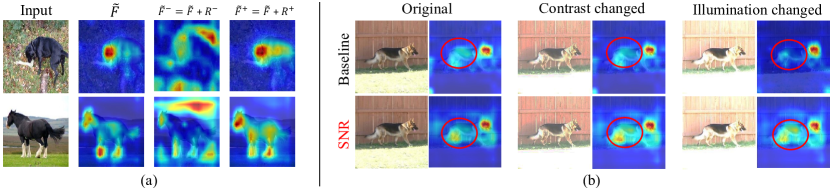
Figure 4: (a) Activation maps of different features within an SNR module (SNR 3). They show that SNR can disentangle out the task-relevant (classification-relevant) object features well (i.e., $R^{+}$). (b) Activation maps of ours (bottom) and the baseline Baseline (AGG) (top) w.r.t images of varied styles. The maps of SNR are more consistent for images of different styles.

Influence of Disentanglement Design. In our SNR module, as described in Eq. (3)(4) of Section III-A2, we use the learned channel attention vector $a(\cdot)$, and its complementary one $1-a(\cdot)$ as masks to obtain task-relevant feature $R^{+}$ and task-irrelevant feature $R^{-}$, respectively. Here, we study the influence of different disentanglement designs within SNR. SNR_conv: we disentangle the residual feature $R$ through 1$\times$1 convolutional layer followed by non-liner ReLU activation, i.e., $R^{+}=ReLU(W^{+}R)$, $R^{-}=ReLU(W^{-}R)$. SNR${{}_{g(\cdot)^{2}}}$: we use two unshared channel attention gates $g(\cdot)^{+}$, $g(\cdot)^{-}$ to obtain $R^{+}$ and $R^{-}$ respectively. SNR-S: different from the original SNR design that leverages channel attention to achieve feature separation, here we disentangle the residual feature $R$ using only a spatial attention, and its complementary. SNR-SC: we disentangle the residual feature $R$ through the paralleled spatial and channel attention. Table VIII shows the results. We have the following observations:

1) Our SNR outperforms SNR_conv by 1.3% on average on PACS, demonstrating the benefit of explicit design of decomposition using attention masks.

2) Ours SNR outperforms SNR${}_{g(\cdot)^{2}}$ by 0.9% on average on PACS, demonstrating the benefit of the design that encourages interaction between $R^{+}$ and $R^{-}$ where their sum is equal to $R$.

3) SNR-S is inferior to SNR that is based on channel attention. Those task-irrelevant style factors (e.g., illumination, contrast, saturation) are in general spatial consistent, which are characterized by the statistics of each channel. IN reduces style discrepancy of input features by performing normalization across spatial dimensions independently for each channel, where the normalization parameters are the same across different spatial positions. Consistent with IN, we disentangle the features at channel level and add the task-relevant ones back to the normalized features.

4) SNR-SC outperforms SNR which uses only channel attention by 0.3% on average on PACS. To be simple and align with our main purpose of distilling the removed task-relevant information, we use only channel attention by default.

TABLE VIII: Study on the disentanglement designs in SNR

Method	PACS
	Art	Cat	Pho	Skt	Avg
Baseline (AGG)	77.0	75.9	96.0	69.2	79.5
SNRconv	77.9	76.4	95.7	71.8	80.5
SNR${}_{g(\cdot)^{2}}$	78.7	76.9	95.2	72.8	80.9
SNR	80.3	78.2	94.5	74.1	81.8
SNR-S	80.1	77.9	94.0	73.6	81.4
SNR-SC	80.7	77.8	94.9	74.8	82.1

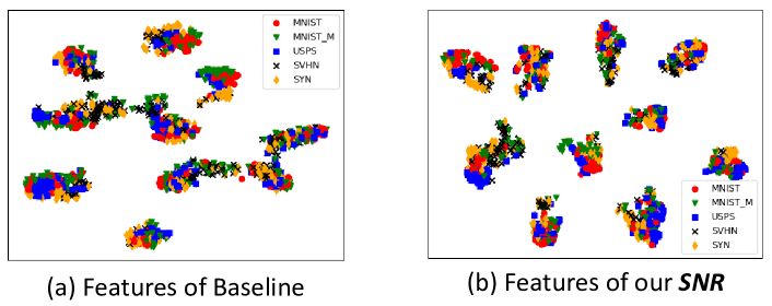
Figure 5: Visualization of t-SNE distributions on the Digit-Five dataset for UDA classification task. We compare our SNR-M3SDA with the baseline scheme Baseline (M3SDA).

IV-A6 Visualization

Feature Map Visualization. To better understand how our SNR works, we visualize the intermediate feature maps of the SNR module that is inserted in the third residual block (i.e., SNR-3). Following [64, 32], we get each activation map by summarizing the feature maps along channels followed by a spatial $\ell_{2}$ normalization.

Fig. 4(a) shows the activation maps of normalized feature $\widetilde{F}$, enhanced feature $\widetilde{F}^{+}=\widetilde{F}+R^{+}$, and contaminated feature $\widetilde{F}^{-}=\widetilde{F}+R^{-}$, respectively. We see that after adding the task-irrelevant feature $R^{-}$, the contaminated feature $\widetilde{F}^{-}$ has high response mainly on background. In contrast, the enhanced feature $\widetilde{F}^{+}$ (with the restitution of task-relevant feature $R^{+}$) has high responses on regions of the object (‘dog’ and ‘horse’), better capturing discriminative feature regions.

Moreover, in Fig. 4(b), we further compare the activation maps $\widetilde{F}^{+}$ of our scheme and those of the strong baseline scheme Baseline (AGG) by varying the styles of input images (e.g., contrast, illumination). We can see that, for the images with different styles, the activation maps of our scheme are more consistent than those of the baseline scheme Baseline (AGG). The activation maps of Baseline (AGG) are more disorganized and are easily affected by style variants. These indicate that our scheme is more robust to style variations.

Visualization of Feature Distributions. In Fig. 5, we visualize the distribution of the features using t-SNE [65] for UDA classification on Digit-Five (on the setting mm,mt,sv,syn$\rightarrow$up). We compare the feature distribution of (a) the baseline scheme Baseline (M3SDA [15]), and (b) our SNR. We observe that the features obtained by our SNR are better separated for different classes than the baseline scheme.

TABLE IX: Domain generalization performance (%) for semantic segmentation when we train on GTA5 and test on Cityscapes.

GTA5$\rightarrow$Cityscape
Setting	Backbone	Method	mIoU	road	sidewalk	building	wall	fence	pole	light	sign	vegetation	terrain	sky	person	rider	car	truck	bus	train	motocycle	bicycle
Source_only	DRN-D-105	Baseline	29.84	45.82	20.80	58.86	5.14	16.74	31.74	33.70	19.34	83.25	15.11	66.99	52.99	9.20	53.59	12.99	14.24	3.46	17.54	5.50
		Baseline-IN	32.64	59.27	16.25	71.58	12.66	16.04	23.61	24.72	14.01	84.43	31.96	62.76	52.33	11.34	61.00	15.27	21.98	7.43	20.48	13.07
		SNR	36.16	83.34	17.32	78.74	16.85	10.71	29.17	30.46	13.76	83.42	34.43	73.30	53.95	8.95	78.84	13.86	15.18	3.96	21.48	19.39
	DeeplabV2	Baseline	36.94	71.41	15.33	74.04	21.13	14.49	22.86	33.93	18.62	80.75	20.98	68.58	56.62	27.17	67.47	32.81	5.60	7.74	28.43	33.82
		Baseline-IN	39.46	73.43	22.19	78.71	24.04	15.29	27.63	29.66	19.96	80.19	27.42	70.26	56.27	15.86	72.97	33.66	37.79	5.63	29.20	29.59
		SNR	42.68	78.95	29.51	79.92	25.01	20.32	28.33	34.83	20.40	82.76	36.13	71.47	59.19	21.62	75.84	32.78	45.48	2.97	30.26	35.13

TABLE X: Domain generalization performance (%) of semantic segmentation when we train on Synthia and test on Cityscapes.

Synthia$\rightarrow$Cityscape
Setting	Backbone	Method	mIoU	road	sidewalk	building	wall	fence	pole	light	sign	vegetation	sky	person	rider	car	bus	motocycle	bicycle
Source_only	DRN-D-105	Baseline	23.56	14.63	11.49	58.96	3.21	0.10	23.80	1.32	7.20	68.49	76.12	54.31	6.98	34.21	15.32	0.81	0.00
		Baseline-IN	24.71	15.89	13.85	63.22	2.98	0.00	26.20	2.56	8.10	70.08	77.52	53.90	7.98	35.62	15.08	2.36	0.00
		SNR	26.30	19.33	15.21	62.54	3.07	0.00	29.15	6.32	10.20	73.22	79.62	53.67	8.92	41.08	15.16	3.23	0.00
	DeeplabV2	Baseline	31.12	35.79	17.12	72.29	4.51	0.15	26.52	5.76	8.23	74.94	80.71	56.18	16.36	39.31	21.57	10.52	27.95
		Baseline-IN	32.93	45.55	23.63	71.68	4.51	0.42	29.36	12.52	14.34	74.94	80.96	50.53	20.15	42.41	11.20	10.30	34.45
		SNR	34.36	50.43	23.64	74.41	5.82	0.37	30.37	12.24	13.52	78.35	83.05	55.29	18.13	47.10	13.73	12.64	30.70

IV-B Semantic Segmentation

IV-B1 Datasets and Implementation Details

For the semantic segmentation task, we used three representative semantic segmentation datasets: Cityscapes [66], Synthia [67], and GTA5 [68]. The detailed datasets introduction and experimental implementation details can be found in Supplementary.

IV-B2 Results on Domain Generalization

Here, we evaluate the effectiveness of SNR under DG setting (only training on the source datasets, and directly testing on the target test set). Since very few previous works investigate on this task, here we define the comparison/validation settings. We compare the proposed scheme SNR with 1) the Baseline (only use source dataset for training) and 2) the baseline when adding IN after each convolutional block Baseline-IN.

Table IX and Table X show that for DRN-D-105, our scheme SNR outperforms Baseline by 6.32% and 2.74% in mIoU accuracy for GTA5-to-Cityscapes and Synthia-to-Cityscapes, respectively. For the stronger backbone network DeeplabV2, our scheme SNR outperforms Baseline by 5.74% and 3.24% in mIoU for GTA5-to-Cityscapes and Synthia-to-Cityscapes, respectively. When compared with the scheme Baseline-IN, our SNR also consistently outperforms it on two backbones for both settings.

TABLE XI: Performance (%) comparisons with the state-of-the-art semantic segmentation approaches for unsupervised domain adaptation for GTA5-to-Cityscape.

GTA5$\rightarrow$Cityscape
Network	method	mIoU	road	sdwk	bldng	wall	fence	pole	light	sign	vgttn	trrn	sky	person	rider	car	truck	bus	train	mcycl	bcycl
DRN-105	DANN  [24]	32.8	64.3	23.2	73.4	11.3	18.6	29.0	31.8	14.9	82.0	16.8	73.2	53.9	12.4	53.3	20.4	11.0	5.0	18.7	9.8
	MCD  [13]	35.0	87.5	17.6	79.7	22.0	10.5	27.5	21.9	10.6	82.7	30.3	78.2	41.1	9.7	80.4	19.3	23.1	11.7	9.3	1.1
	SNR-MCD (ours)	40.3	87.7	36.0	80.0	19.7	19.1	30.9	32.4	13.0	82.8	34.9	79.1	50.3	11.0	84.3	23.0	28.6	16.8	18.5	17.9
DeeplabV2	AdaptSegNet  [69]	42.4	86.5	36.0	79.9	23.4	23.3	23.9	35.2	14.8	83.4	33.3	75.6	58.5	27.6	73.7	32.5	35.4	3.9	30.1	28.1
	MinEnt  [70]	42.3	86.2	18.6	80.3	27.2	24.0	23.4	33.5	24.7	83.3	31.0	75.6	54.6	25.6	85.2	30.0	10.9	0.1	21.9	37.1
	AdvEnt+MinEnt  [70]	44.8	87.6	21.4	82.0	34.8	26.2	28.5	35.6	23.0	84.5	35.1	76.2	58.6	30.7	84.8	34.2	43.4	0.4	28.4	35.3
	MaxSquare (MS)  [71]	44.3	88.1	27.7	80.8	28.7	19.8	24.9	34.0	17.8	83.6	34.7	76.0	58.6	28.6	84.1	37.8	43.1	7.2	32.2	34.2
	SNR-MS (ours)	46.5	90.8	40.9	81.6	29.8	23.5	24.4	34.1	21.6	84.0	39.6	77.0	59.3	30.9	84.4	37.8	44.6	8.5	33.2	37.9

TABLE XII: Performance (%) comparisons with the state-of-the-art semantic segmentation approaches for unsupervised domain adaptation for Synthia-to-Cityscape.

Synthia$\rightarrow$Cityscape
Network	method	mIoU	road	sdwk	bldng	wall	fence	pole	light	sign	vgttn	trrn	sky	person	car	bus	mcycl	bcycl
DRN-105	DANN  [24]	32.5	67.0	29.1	71.5	14.3	0.1	28.1	12.6	10.3	72.7	76.7	48.3	12.7	62.5	11.3	2.7	0.0
	MCD  [13]	36.6	84.5	43.2	77.6	6.0	0.1	29.1	7.2	5.6	83.8	83.5	51.5	11.8	76.5	19.9	4.7	0.0
	SNR-MCD (ours)	39.6	88.1	55.4	71.7	16.3	0.2	27.6	13.0	11.3	82.4	82.0	55.0	13.7	83.3	27.8	6.7	0.0
DeeplabV2	AdaptSegNet  [69]	-	84.3	42.7	77.5	-	-	-	4.7	7.0	77.9	82.5	54.3	21.0	72.3	32.2	18.9	32.3
	MinEnt  [70]	38.1	73.5	29.2	77.1	7.7	0.2	27.0	7.1	11.4	76.7	82.1	57.2	21.3	69.4	29.2	12.9	27.9
	AdvEnt+MinEnt  [70]	41.2	85.6	42.2	79.7	8.7	0.4	25.9	5.4	8.1	80.4	84.1	57.9	23.8	73.3	36.4	14.2	33.0
	MaxSquare (MS)  [71]	39.3	77.4	34.0	78.7	5.6	0.2	27.7	5.8	9.8	80.7	83.2	58.5	20.5	74.1	32.1	11.0	29.9
	SNR-MS (ours)	45.1	90.0	37.1	82.0	10.3	0.9	27.4	15.1	26.3	82.9	76.6	60.5	26.6	86.0	41.3	31.6	27.6

IV-B3 Results on Unsupervised Domain Adaptation

Unsupervised domain adaptive semantic segmentation has been extensively studied [13, 71], where the unlabeled target domain data is also used for training. We validate the effectiveness of UDA by adding the SNR modules into two popular UDA approaches: MCD [13] and MaxSqure(MS) [71], respectively. MCD [13] maximizes the discrepancy between two task-classifiers while minimizing it with respect to the feature extractor of domain adaptation. MS  [71] extends the entropy minimization idea to UDA for semantic segmentation by using a proposed maximum squares loss. We refer to the two schemes powered by our SNR modules as SNR-MCD and SNR-MS. Table XI and Table XII show that based on the same DRN-105 backbone, SNR-MCD significantly outperforms the second-best method MCD [13] by 5.3%, and 3.0% in mIoU for GTA5$\rightarrow$Cityscape and Synthia$\rightarrow$Cityscape, respectively. In addition, based on the DeeplabV2 backbone, SNR-MS consistently outperforms MaxSqure (MS) [71] by 2.2%, and 5.8% in mIoU for GTA5$\rightarrow$Cityscape and Synthia$\rightarrow$Cityscape, respectively.

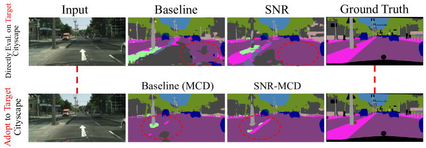
Figure 6: Qualitative results on domain generable segmentation (first row) and domain adaptive segmentation (second row) from GTA5 to Cityscapes. For DG (first row), Baseline denotes the baseline scheme trained with source domain dataset while testing on the target domain directly. SNR denotes our scheme which adds SNR modules to Baseline. For UDA (second row), we compare the baseline scheme Baseline (MCD) [13] to the scheme SNR+MCD which is powered by our SNR.

IV-B4 Visualization of DG and UDA Results

We visualize the qualitative results in Fig. 6 by comparing the baseline schemes and the schemes powered by our SNR. For DG in the first row, we can see that the introduction of SNR to Baseline brings obvious improvement on the segmentation results. For UDA in the second row, 1) the introduction of SNR to Baseline (MCD) brings clear improvement on the segmentation results; 2) the segmentation results with adapation (UDA) to the target domain data is much better than that obtained from domain generalization model, indicating the exploration of target domain data is helpful to have good performance.

IV-C Object Detection

IV-C1 Datasets and Implementation Details

Following [72, 73], we evaluate performance on multi- and single-label object detection tasks using three different datasets: Cityscapes [66], Foggy Cityscapes [74], and KITTI [75]. The detailed datasets introduction can be found in Supplementary.

TABLE XIII: Performance (in mAP accuracy %) of object detection on the Foggy Cityscapes validation set, models are trained on the Cityscapes training set.

Setting	Method	Cityscapes$\rightarrow$Foggy Cityscapes
		person	rider	car	truck	bus	train	mcycle	bicycle	mAP
DG	Faster R-CNN [52]	17.8	23.6	27.1	11.9	23.8	9.1	14.4	22.8	18.8
	SNR-Faster R-CNN	20.3	24.6	33.6	15.9	26.3	14.4	16.8	26.8	22.3
UDA	DA Faster R-CNN [72]	25.0	31.0	40.5	22.1	35.3	20.2	20.0	27.1	27.6
	SNR-DA Faster R-CNN	27.3	34.6	44.6	23.9	38.1	25.4	21.3	29.7	30.6

TABLE XIV: Performance (in AP accuracy %) for the class of Car for object detection on KITTI (K) and Cityscapes (C).

Setting	Method	K$\rightarrow$C	C$\rightarrow$K
DG	Faster R-CNN [52]	30.24	53.52
	SNR	35.92	57.94
UDA	DA Faster R-CNN [72]	38.52	64.15
	SNR	43.51	69.17

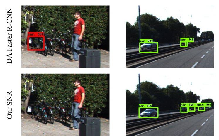
Figure 7: Qualitative comparisons of the baseline approach DA Faster R-CNN  [72] and the baseline powered by our SNR on “Cityscapes $\rightarrow$ KITTI”. Top and bottom rows denote the detected cars by the baseline scheme DA Faster R-CNN and our scheme SNR-DA Faster R-CNN respectively.

TABLE XV: Comparisons of complexity and model sizes. FLOPs: the number of FLoating-point OPerations; Params: the number of parameter.

	FLOPs	Params
ResNet-18	1.83G	11.74M
ResNet-18-SNR	2.03G	12.30M
$\Delta$	+9.80%	+4.50%
ResNet-50	3.87G	24.56M
ResNet-50-SNR	4.08G	25.12M
$\Delta$	+5.10%	+2.20%

For the domain generalization (DG) experiments, we employ the original Faster RCNN [52] as our baseline, which is trained using the source domain training data. We follow [52] to set the hyper-parameters. For our scheme SNR, we add SNR modules into the backbone (by adding a SNR module after each convolutional block for the first four blocks of ResNet-50) of the Faster RCNN, which are initialized using weights pre-trained on ImageNet. We train the network with a learning rate of $0.001$ for $50$k iterations and then reduce the learning rate to $0.0001$ for another $20$k iterations.

For the unsupervised domain adaptation (UDA) experiments, we use the Domain Adaptive Faster R-CNN (Da Faster R-CNN) [72] model as our baseline, which tackles the domain shift on two levels, the image level and the instance level. A domain classifier is added on each level, trained in an adversarial training manner. A consistency regularizer is incorporated within these two classifiers to learn a domain-invariant RPN for the Faster R-CNN model. Each batch is composed of two images, one from the source domain and the other from the target domain. A momentum of 0.9 and a weight decay of 0.0005 is used in our experiments.

For all experiments , we report mean average precisions (mAP) with a threshold of 0.5 for evaluation.

IV-C2 Results on DG and UDA

Results for Normal to Foggy Weather. Differences in weather conditions can significantly affect visual data. In many applications (i.e., autonomous driving), the object detector needs to perform well in all conditions [74]. Here we evaluate the effectiveness of our SNR and demonstrate its generalization superiority over the current state-of-the-art for this task. We use Cityscapes dataset as the source domain and Foggy Cityscapes as the target domain (denoted by “Cityscapes $\rightarrow$ Foggy Cityscapes”).

Table XIII compares our schemes using SNR to two baselines (Faster R-CNN [52], and Domain Adaptive (DA) Faster R-CNN [72]) on domain generalization, and domain adaptation settings. We report the average precision for each category, and the mean average precision (mAP) of all the objects. We can see that our SNR improves Faster R-CNN by $3.5\%$ in mAP for domain generalization, and improves DA Faster R-CNN by $3.0\%$ in mAP for unsupervised domain adaptation.

Results for Cross-Dataset DG and UDA. Many factors could result in domain gaps. There is usually some data bias when collecting the datasets [76]. For example, different datasets are usually captured by different cameras or collected by different organizations with different preference, with different image quality/resolution/characteristics. In this subsection, we conduct experiments on two datasets: Cityscapes and KITTI. We only train the detector on annotated cars because cars is the only object common to both Cityscapes and KITTI.

Table XIV compares our methods to two baselines: Faster R-CNN [52], and Domain Adaptive (DA) Faster R-CNN [72] for domain generalization and domain adaptation setting, respectively. We denote KITTI (source dataset) to Cityscapes (target dataset) as $K\rightarrow C$ and vice versa. We can see that the introduction of SNR brings significant performance improvement for both DG and UDA settings.

IV-C3 Qualitative Results

For UDA, we visualize the qualitative detection results in Fig. 7. We see that our SNR corrects several false positives in the first column, and has detected cars that DA Faster R-CNN missed in the second column.

IV-D Complexity Analysis

In Table XV, we analyze the increase of complexity of our SNR modules in terms of FLOPs and model size with respect to different backbone networks. Here, we use our default setting where we insert a SNR module after each convolutional block (for the first four blocks) for the backbone networks of ResNet-18, ResNet-50. We observe that our SNR modules bring a small increase in complexity. For ResNet-50 [49] backbone, our SNR only brings an increase of 2.2% in model size (24.56M vs. 25.12M) and an increase of 5.1% in computational complexity (3.87G vs. 4.08G FLOPs).

V Conclusion

In this paper, we present a Style Normalization and Restitution (SNR) module, which aims to learn generalizable and discriminative feature representations for effective domain generalization and adaptation. SNR is generic. As a plug-and-play module, it can be inserted into existing backbone networks for many computer vision tasks. SNR reduces the style variations by using Instance Normalization (IN). To prevent the loss of task-relevant discriminative information cased by IN, we propose to distill task-relevant discriminative features from the discarded residual features and add them back to the network, through a well-designed restitution step. Moreover, to promote a better feature disentanglement of task-relevant and task-irrelevant information, we introduce a dual restitution loss constraint. Extensive experimental results demonstrate the effectiveness of our SNR module for both domain generalization and domain adaptation. The schemes powered by SNR achieves the state-of-the-art performance on various tasks, including classification, semantic segmentation, and object detection.

Appendix

VI Datasets and Implementation Details

VI-A Object Classification

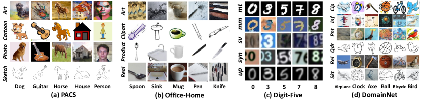
Figure 8: Four classification datasets (first two for DG and last two for UDA). (a) PACS, which includes Sketch, Photo, Cartoon, and Art. (b) Office-Home, which includes Real-world (Real), Product, Clipart, and Art. (c) Digit-Five, which includes MNIST [59] (mt), MNIST-M [60] (mm), USPS [61] (up), SVHN [62] (sv), and Synthetic [60] (syn). (d) DomainNet, which includes Clipart (clp), Infograph (inf), Painting (pnt), Quickdraw (qdr), Real (rel), and Sktech (skt). Considering the required huge computation resources, we use a subset of DomainNet (i.e., mini-DomainNet) following [31] for ablation experiments. The full DomainNet dataset is also used for performance comparison with the state-of-the-art methods.

Fig. 8 shows some samples of these datasets. PACS [5] and Office-Home [77] are two widely used DG datasets where each dataset includes four domains. PACS has seven object categories and office-Home has 65 categories. Digit-Five consists of five different digit recognition datasets: MNIST [59], MNIST-M [60], USPS [61], SVHN [62] and SYN [60]. We follow the same split setting as [15] to use the dataset. DomainNet is a recently introduced benchmark for large-scale multi-source domain adaptation [15], which includes six domains (i.e., Clipart, Infograph, Painting, Quickdraw, Real, and Sketch) of 600k images (345 classes). Considering the high demand on computational resources, following [31], we use a subset of DomainNet, i.e., mini-DomainNet, for ablation experiments. The full DomainNet dataset is also used for performance comparison with the state-of-the-art methods.

PACS and Office-Home are usually used for DG. We validate the effectiveness of DG on PACS and Office-Home. Following [15], we use the leave-one-domain-out protocol. For PACS and Office-Home, similar to [78, 9], we use ResNet18 as the backbone to build our baseline network. We train the model for 40 epochs with an initial learning rate of 0.002. Each mini-batch contains 30 images (10 per source domain). We insert a SNR module after each convolutional block of the ResNet18 baseline as our SNR scheme.

Digit-5 and DomainNet are usually used for DA. We validate the effectiveness of our DA on them. We follow prior works [5, 78, 9] to use the leave-one-domain-out protocol. For Digit-5, following [15], we build the backbone with three convolution layers and two fully connected layers. We insert a SNR module after each convolutional layer of the baseline as our SNR scheme. For each mini-batch, we sample 64 images from each domain. The model is trained with an initial learning rate of 0.05 for 30 epochs. For mini-DomainNet, we use ResNet18 [49] as the backbone. For full DomainNet, we use ResNet152 [49] as the backbone. We insert a SNR module after each convolutional block of the ResNet baseline as our SNR scheme. We sample 32 images from each domain to form a mini-batch (of size 32$\times$4=128) and train the model for 60 epochs with an initial learning rate of 0.005. In all experiments, SGD with momentum is used as the optimizer and a cosine annealing rule [79] is adopted for learning rate decay.

VI-B Semantic Segmentation

Cityscapes contains 5,000 annotated images with 2048$\times$1024 resolution captured from real urban street scenes. GTA5 contains 24,966 annotated images with 1914$\times$1052 resolution obtained from the GTA5 game. For SYNTHIA, we use the subset SYNTHIA-RAND-CITYSCAPES which consists of 9,400 synthetic images of resolution 1280$\times$760.

Following the prior works [80, 81, 13], we use the labeled training set of GTA5 or SYNTHIA as the source domain and the Cityscapes validation set as our test set. We adopt the Intersection-over-Union (IoU) of each class and the mean-Intersection-over-Union (mIoU) as evaluation metrics. We consider the IoU and mIoU of all the 19 classes in the GTA5-to-Cityscapes case. Since SYNTHIA has only 16 shared classes with Cityscapes, we consider the IoU and mIoU of the 16 classes in the SYNTHIA-to-Cityscapes setting.

As discussed in [69, 71], it is also important to adopt a stronger baseline model to understand the effect of different generalization/adaption approaches and to enhance the performance for the practical applications. Therefore, similar to [13], in all experiments, we employ two kinds of backbones for evaluation.

1) We use DRN-D-105 [82, 13] as our baseline network and apply our SNR to the network. For DRN-D-105, we follow the implementation of MCD. Similiar to ResNet [49], DRN still uses the block-based architecture. We insert our SNR module after each convolutional block of DRN-D-105. We use momentum SGD to optimize our models. We set the momentum rate to 0.9 and the learning rate to 10e-3 in all experiments. The image size is resized to 1024$\times$512. Here, we report the output results obtained after 50,000 iterations.

2) We also use Deeplabv2 [83] with ResNet-101 [84] backbone that is pre-trained on ImageNet [85] as our baseline network, which is the same as other works [86, 87]. We insert our SNR module after each convolutional block of ResNet-101. Following the implementation of MSL [71], we train the model with SGD optimizer with the learning rate $2.5\times 10^{-4}$, momentum $0.9$, and weight decay $5\times 10^{-4}$. We schedule the learning rate using “poly" policy: the learning rate is multiplied by $(1-\frac{iter}{max\_iter})^{0.9}$ [83]. Similar to [88], we employ the random flipping and Gaussian blur for data augmentation.

VI-C Object Detection

Cityscapes [66] is a dataset of real urban scenes containing $3,475$ images captured by a dash-cam. $2,975$ images are used for training and the remaining $500$ for validation (such split information is different from the above-mentioned statistics for the semantic segmentation). Following  [72], we report results on the validation set because we do not have annotations of the test set. There are $8$ different object categories in this dataset including person, rider, car, truck, bus, train, motorcycle and bicycle.

Foggy Cityscapes [74] is the foggy version of Cityscapes. The depth maps provided in Cityscapes are used to simulate three intensity levels of fog in [74]. In our experiments we used the fog level with highest intensity (least visibility) to imitate large domain gap. The same dataset split as used for Cityscapes is used for Foggy Cityscapes.

KITTI [75] is another real-world dataset consisting of $7,481$ images of real-world traffic situations, including freeways, urban and rural areas. Following [72], we use the entire dataset for training, when it is used as source. We use the entire dataset for testing when it is used as target test set for DG.

References

- [1] A. Krizhevsky, I. Sutskever, and G. E. Hinton, “Imagenet classification with deep convolutional neural networks,” in NeurIPS, 2012, pp. 1097–1105.
- [2] M. Long, H. Zhu, J. Wang, and M. I. Jordan, “Unsupervised domain adaptation with residual transfer networks,” in NeurIPS, 2016, pp. 136–144.
- [3] X. Ma, T. Zhang, and C. Xu, “Deep multi-modality adversarial networks for unsupervised domain adaptation,” IEEE TMM, vol. 21, no. 9, pp. 2419–2431, 2019.
- [4] K. Muandet, D. Balduzzi, and B. Schölkopf, “Domain generalization via invariant feature representation,” in International Conference on Machine Learning, 2013, pp. 10–18.
- [5] D. Li, Y. Yang, Y.-Z. Song, and T. M. Hospedales, “Deeper, broader and artier domain generalization,” in ICCV, 2017, pp. 5542–5550.
- [6] S. Shankar, V. Piratla, S. Chakrabarti, S. Chaudhuri, P. Jyothi, and S. Sarawagi, “Generalizing across domains via cross-gradient training,” ICLR, 2018.
- [7] D. Li, Y. Yang, Y.-Z. Song, and T. M. Hospedales, “Learning to generalize: Meta-learning for domain generalization,” in AAAI, 2018.
- [8] F. M. Carlucci, A. D’Innocente, S. Bucci, B. Caputo, and T. Tommasi, “Domain generalization by solving jigsaw puzzles,” in CVPR, 2019, pp. 2229–2238.
- [9] D. Li, J. Zhang, Y. Yang, C. Liu, Y.-Z. Song, and T. M. Hospedales, “Episodic training for domain generalization,” in ICCV, 2019, pp. 1446–1455.
- [10] S. J. Pan and Q. Yang, “A survey on transfer learning,” IEEE Transactions on knowledge and data engineering, vol. 22, no. 10, pp. 1345–1359, 2009.
- [11] Y. Ganin and V. Lempitsky, “Unsupervised domain adaptation by backpropagation,” ICML, 2014.
- [12] M. Long, Y. Cao, J. Wang, and M. I. Jordan, “Learning transferable features with deep adaptation networks,” ICML, 2015.
- [13] K. Saito, K. Watanabe, Y. Ushiku, and T. Harada, “Maximum classifier discrepancy for unsupervised domain adaptation,” in CVPR, 2018, pp. 3723–3732.
- [14] J. Hoffman, E. Tzeng, T. Park, J.-Y. Zhu, P. Isola, K. Saenko, A. A. Efros, and T. Darrell, “Cycada: Cycle-consistent adversarial domain adaptation,” ICML, 2018.
- [15] X. Peng, Q. Bai, X. Xia, Z. Huang, K. Saenko, and B. Wang, “Moment matching for multi-source domain adaptation,” in ICCV, 2019, pp. 1406–1415.
- [16] R. Xu, G. Li, J. Yang, and L. Lin, “Larger norm more transferable: An adaptive feature norm approach for unsupervised domain adaptation,” in ICCV, 2019, pp. 1426–1435.
- [17] X. Wang, Y. Jin, M. Long, J. Wang, and M. I. Jordan, “Transferable normalization: Towards improving transferability of deep neural networks,” in NeurIPS, 2019, pp. 1951–1961.
- [18] B. Sun, J. Feng, and K. Saenko, “Return of frustratingly easy domain adaptation,” in AAAI, 2016.
- [19] B. Sun and K. Saenko, “Deep coral: Correlation alignment for deep domain adaptation,” in ECCV, 2016, pp. 443–450.
- [20] X. Peng and K. Saenko, “Synthetic to real adaptation with generative correlation alignment networks,” in WACV. IEEE, 2018, pp. 1982–1991.
- [21] W. Zellinger, T. Grubinger, E. Lughofer, T. Natschläger, and S. Saminger-Platz, “Central moment discrepancy (cmd) for domain-invariant representation learning,” CoRR, 2017.
- [22] E. Tzeng, J. Hoffman, N. Zhang, K. Saenko, and T. Darrell, “Deep domain confusion: Maximizing for domain invariance,” arXiv preprint arXiv:1412.3474, 2014.
- [23] M. Long, H. Zhu, J. Wang, and M. I. Jordan, “Deep transfer learning with joint adaptation networks,” in ICML, 2017, pp. 2208–2217.
- [24] Y. Ganin, E. Ustinova, H. Ajakan, P. Germain, H. Larochelle, F. Laviolette, M. Marchand, and V. Lempitsky, “Domain-adversarial training of neural networks,” The Journal of Machine Learning Research, vol. 17, no. 1, pp. 2096–2030, 2016.
- [25] E. Tzeng, J. Hoffman, K. Saenko, and T. Darrell, “Adversarial discriminative domain adaptation,” in CVPR, 2017, pp. 7167–7176.
- [26] H. Liu, M. Long, J. Wang, and M. Jordan, “Transferable adversarial training: A general approach to adapting deep classifiers,” in ICML, 2019, pp. 4013–4022.
- [27] M. Ghifary, D. Balduzzi, W. B. Kleijn, and M. Zhang, “Scatter component analysis: A unified framework for domain adaptation and domain generalization,” TPAMI, vol. 39, no. 7, pp. 1414–1430, 2016.
- [28] S. Motiian, M. Piccirilli, D. A. Adjeroh, and G. Doretto, “Unified deep supervised domain adaptation and generalization,” in ICCV, 2017, pp. 5715–5725.
- [29] J. Jia, Q. Ruan, and T. M. Hospedales, “Frustratingly easy person re-identification: Generalizing person re-id in practice,” 2019.
- [30] J. Song, Y. Yang, Y.-Z. Song, T. Xiang, and T. M. Hospedales, “Generalizable person re-identification by domain-invariant mapping network,” 2019.
- [31] K. Zhou, Y. Yang, Y. Qiao, and T. Xiang, “Domain adaptive ensemble learning,” arXiv preprint arXiv:2003.07325, 2020.
- [32] K. Zhou, Y. Yang, A. Cavallaro et al., “Omni-scale feature learning for person re-identification,” 2019.
- [33] X. Huang and S. Belongie, “Arbitrary style transfer in real-time with adaptive instance normalization,” in ICCV, 2017, pp. 1501–1510.
- [34] X. Pan, P. Luo, J. Shi, and X. Tang, “Two at once: Enhancing learning and generalization capacities via ibn-net,” in ECCV, 2018, pp. 464–479.
- [35] D. Ulyanov, A. Vedaldi, and V. Lempitsky, “Improved texture networks: Maximizing quality and diversity in feed-forward stylization and texture synthesis,” in CVPR, 2017, pp. 6924–6932.
- [36] V. Dumoulin, J. Shlens, and M. Kudlur, “A learned representation for artistic style,” ICLR, 2017.
- [37] X. Jin, C. Lan, W. Zeng, Z. Chen, and L. Zhang, “Style normalization and restitution for generalizable person re-identification,” arXiv preprint arXiv:2005.11037, 2020.
- [38] R. Volpi, H. Namkoong, O. Sener, J. C. Duchi, V. Murino, and S. Savarese, “Generalizing to unseen domains via adversarial data augmentation,” in NeurIPS, 2018, pp. 5334–5344.
- [39] D. Ulyanov, A. Vedaldi, and V. Lempitsky, “Instance normalization: The missing ingredient for fast stylization,” arXiv preprint arXiv:1607.08022, 2016.
- [40] H. Bilen and A. Vedaldi, “Universal representations: The missing link between faces, text, planktons, and cat breeds,” arXiv preprint arXiv:1701.07275, 2017.
- [41] H. Nam and H.-E. Kim, “Batch-instance normalization for adaptively style-invariant neural networks,” in NeurIPS, 2018, pp. 2558–2567.
- [42] H. Yan, Z. Li, Q. Wang, P. Li, Y. Xu, and W. Zuo, “Weighted and class-specific maximum mean discrepancy for unsupervised domain adaptation,” IEEE TMM, vol. 22, no. 9, pp. 2420–2433, 2019.
- [43] W. Zhang, W. Ouyang, W. Li, and D. Xu, “Collaborative and adversarial network for unsupervised domain adaptation,” in CVPR, 2018, pp. 3801–3809.
- [44] H. Zhao, S. Zhang, G. Wu, J. M. Moura, J. P. Costeira, and G. J. Gordon, “Adversarial multiple source domain adaptation,” in NeurIPS, 2018, pp. 8559–8570.
- [45] K. Saito, D. Kim, S. Sclaroff, T. Darrell, and K. Saenko, “Semi-supervised domain adaptation via minimax entropy,” in ICCV, 2019, pp. 8050–8058.
- [46] X. Peng, Z. Huang, Y. Zhu, and K. Saenko, “Federated adversarial domain adaptation,” ICLR, 2020.
- [47] A. H. Liu, Y.-C. Liu, Y.-Y. Yeh, and Y.-C. F. Wang, “A unified feature disentangler for multi-domain image translation and manipulation,” in NeurIPS, 2018, pp. 2590–2599.
- [48] H.-Y. Lee, H.-Y. Tseng, J.-B. Huang, M. Singh, and M.-H. Yang, “Diverse image-to-image translation via disentangled representations,” in ECCV, 2018, pp. 35–51.
- [49] K. He, X. Zhang, S. Ren, and J. Sun, “Deep residual learning for image recognition,” in CVPR, 2016.
- [50] J. Hu, L. Shen, and G. Sun, “Squeeze-and-excitation networks,” in CVPR, 2018, pp. 7132–7141.
- [51] R. Girshick, J. Donahue, T. Darrell, and J. Malik, “Rich feature hierarchies for accurate object detection and semantic segmentation,” in CVPR, 2014, pp. 580–587.
- [52] S. Ren, K. He, R. Girshick, and J. Sun, “Faster r-cnn: Towards real-time object detection with region proposal networks,” in NeurIPS, 2015, pp. 91–99.
- [53] K. He, G. Gkioxari, P. Dollár, and R. Girshick, “Mask r-cnn,” in ICCV, 2017, pp. 2961–2969.
- [54] H. Li, S. Jialin Pan, S. Wang, and A. C. Kot, “Domain generalization with adversarial feature learning,” in CVPR, 2018, pp. 5400–5409.
- [55] K. Zhou, Y. Yang, T. Hospedales, and T. Xiang, “Learning to generate novel domains for domain generalization,” in ECCV. Springer, 2020, pp. 561–578.
- [56] R. Xu, Z. Chen, W. Zuo, J. Yan, and L. Lin, “Deep cocktail network: Multi-source unsupervised domain adaptation with category shift,” in CVPR, 2018, pp. 3964–3973.
- [57] J. Wang, W. Feng, Y. Chen, H. Yu, M. Huang, and P. S. Yu, “Visual domain adaptation with manifold embedded distribution alignment,” in ACMMM, 2018, pp. 402–410.
- [58] H. Venkateswara, J. Eusebio, S. Chakraborty, and S. Panchanathan, “Deep hashing network for unsupervised domain adaptation,” in CVPR, 2017.
- [59] Y. LeCun, L. Bottou, Y. Bengio, and P. Haffner, “Gradient-based learning applied to document recognition,” in IEEE, 1998.
- [60] Y. Ganin and V. S. Lempitsky, “Unsupervised domain adaptation by backpropagation,” in ICML, 2015.
- [61] J. J. Hull, “A database for handwritten text recognition research,” TPAMI, vol. 16, no. 5, pp. 550–554, 1994.
- [62] Y. Netzer, T. Wang, A. Coates, A. Bissacco, B. Wu, and A. Y. Ng, “Reading digits in natural images with unsupervised feature learning,” in NeurIPS-W, 2011.
- [63] S. Ioffe and C. Szegedy, “Batch normalization: Accelerating deep network training by reducing internal covariate shift,” arXiv preprint arXiv:1502.03167, 2015.
- [64] W.-S. Zheng, S. Gong, and T. Xiang, “Person re-identification by probabilistic relative distance comparison,” 2011.
- [65] L. v. d. Maaten and G. Hinton, “Visualizing data using t-sne,” 2008.
- [66] M. Cordts, M. Omran, S. Ramos, T. Rehfeld, M. Enzweiler, R. Benenson, U. Franke, S. Roth, and B. Schiele, “The cityscapes dataset for semantic urban scene understanding,” in CVPR, 2016.
- [67] G. Ros, L. Sellart, J. Materzynska, D. Vazquez, and A. M. Lopez, “The synthia dataset: A large collection of synthetic images for semantic segmentation of urban scenes,” in CVPR, 2016, pp. 3234–3243.
- [68] S. R. Richter, V. Vineet, S. Roth, and V. Koltun, “Playing for data: Ground truth from computer games,” in ECCV, ser. LNCS, B. Leibe, J. Matas, N. Sebe, and M. Welling, Eds., vol. 9906. Springer International Publishing, 2016, pp. 102–118.
- [69] Y.-H. Tsai, W.-C. Hung, S. Schulter, K. Sohn, M.-H. Yang, and M. Chandraker, “Learning to adapt structured output space for semantic segmentation,” in CVPR, 2018, pp. 7472–7481.
- [70] T.-H. Vu, H. Jain, M. Bucher, M. Cord, and P. Pérez, “Advent: Adversarial entropy minimization for domain adaptation in semantic segmentation,” in CVPR, 2019, pp. 2517–2526.
- [71] M. Chen, H. Xue, and D. Cai, “Domain adaptation for semantic segmentation with maximum squares loss,” in ICCV, 2019, pp. 2090–2099.
- [72] Y. Chen, W. Li, C. Sakaridis, D. Dai, and L. Van Gool, “Domain adaptive faster r-cnn for object detection in the wild,” in CVPR, 2018, pp. 3339–3348.
- [73] M. Khodabandeh, A. Vahdat, M. Ranjbar, and W. G. Macready, “A robust learning approach to domain adaptive object detection,” in ICCV, 2019, pp. 480–490.
- [74] C. Sakaridis, D. Dai, and L. Van Gool, “Semantic foggy scene understanding with synthetic data,” IJCV, pp. 1–20, 2018.
- [75] A. Geiger, P. Lenz, C. Stiller, and R. Urtasun, “Vision meets robotics: The kitti dataset,” IJRR, 2013.
- [76] A. Torralba and A. A. Efros, “Unbiased look at dataset bias,” in CVPR 2011. IEEE, 2011, pp. 1521–1528.
- [77] H. Venkateswara, J. Eusebio, S. Chakraborty, and S. Panchanathan, “Deep hashing network for unsupervised domain adaptation,” in CVPR, 2017.
- [78] F. M. Carlucci, A. D’Innocente, S. Bucci, B. Caputo, and T. Tommasi, “Domain generalization by solving jigsaw puzzles,” in CVPR, 2019.
- [79] I. Loshchilov and F. Hutter, “Sgdr: Stochastic gradient descent with warm restarts,” in ICLR, 2017.
- [80] J. Hoffman, D. Wang, F. Yu, and T. Darrell, “Fcns in the wild: Pixel-level adversarial and constraint-based adaptation,” arXiv preprint arXiv:1612.02649, 2016.
- [81] Y. Zhang, P. David, and B. Gong, “Curriculum domain adaptation for semantic segmentation of urban scenes,” in ICCV, 2017, pp. 2020–2030.
- [82] F. Yu, V. Koltun, and T. Funkhouser, “Dilated residual networks,” in CVPR, 2017, pp. 472–480.
- [83] L. Chen, G. Papandreou, I. Kokkinos, K. Murphy, and A. L. Yuille, “Deeplab: Semantic image segmentation with deep convolutional nets, atrous convolution, and fully connected crfs,” CoRR, vol. abs/1606.00915, 2016.
- [84] K. He, X. Zhang, S. Ren, and J. Sun, “Deep residual learning for image recognition,” in CVPR, 2016.
- [85] J. Deng, W. Dong, R. Socher, L. Li, K. Li, and F. Li, “Imagenet: A large-scale hierarchical image database,” in CVPR, 2009.
- [86] Y. Tsai, W. Hung, S. Schulter, K. Sohn, M. Yang, and M. Chandraker, “Learning to adapt structured output space for semantic segmentation,” in CVPR, 2018.
- [87] T. Vu, H. Jain, M. Bucher, M. Cord, and P. Pérez, “ADVENT: adversarial entropy minimization for domain adaptation in semantic segmentation,” CoRR, vol. abs/1811.12833, 2018.
- [88] H. Zhao, J. Shi, X. Qi, X. Wang, and J. Jia, “Pyramid scene parsing network,” in CVPR, 2017, pp. 2881–2890.