Polarized radiation and the Emergence of Biological Homochirality on Earth and Beyond
Abstract
It has been proposed that spin-polarized cosmic radiation can induce asymmetric changes in helical biopolymers that may account for the emergence of biological homochirality. The parity violation in the weak interaction has direct consequences on the transport of polarization in cosmic ray showers. In this paper, we show that muons retain their polarization down to energies at which they can initiate enantioselective mutagenesis. Therefore, muons are most likely to succeed in establishing the connection between broken symmetries in the standard model of particle physics and that found in living organisms. We calculate the radiation doses deposited by primary and secondary cosmic rays at various prime targets for the searches of life in the solar system: Mars, Venus, Titan, icy moons and planetesimals, and discuss the implications for the enantioselective mutagenesis proposed as to be the driver of homochiralization. Earth is unusual in that spin-polarized muons dominate the cosmic radiation at its surface.
1 Introduction
The origin of life is still a puzzle. However, it is a chiral puzzle: living organisms use only one class of enantiomer (molecule that has a mirror image) in the construction of proteins and nucleic acids, a fundamental property of life known as homochirality (see Avnir, 2020, for a recent review). Homochirality allows biopolymers to adopt stable helical structures (Bada, 1995; Nanda et al., 2007), a natural conformation for biological macromolecules to adopt and one that plays a key role in fundamental biological processes (Totsingan et al., 2012). While helical biopolymers have not been found, yet, in extraterrestrial environments, enantiomeric excesses (e.e.) of a few percent have been reported in the amino acids content of some meteorites (Pizzarello, 2006; Burton & Berger, 2018), but their relation to biological homochirality remains a mystery.
An important clue pertaining to the emergence of homochirality comes from studies of low energy, spin-polarized electrons which can promote enantioselective chemistry (e.g., Dreiling & Gay, 2014; Rosenberg, 2019). In addition, the Chirality-Induced Spin Selectivity, CISS, effect shows that helical biopolymers, specifically double strand DNA and -helical peptide, can act as spin filters for sub-eV electrons (Naaman & Waldeck, 2012). This may be related to biological function and may play a role in the emergence of homochirality.
Cosmic rays, play a major role in generating mutation and promoting evolution on Earth. They create pions in the upper atmosphere which decay into highly polarized muons which comprise the most prevalent high energy particles at ground level. Muons decay into electrons and positrons which are also polarized. In Globus & Blandford (2020), henceforth GB20, it was proposed that this polarization could impose a small chiral preference on the development of one set of biological enantiomers over the other which could evolve to homochirality over millions or even billions of generations. Some mechanisms for expressing this preference were discussed, supplying a causal connection from a fundamental physics asymmetry to an equally fundamental asymmetry in biology.
There are three stages to this scheme: I. Understanding cosmic ray polarization in different environments, II. Estimating the chiral preference present in the mutation rate with a given irradiation and III. Translating this into an influence on biological evolution. In GB20, the focus was on stage II and some semi-classical models of the interaction between cosmic rays and a chiral distribution of electrons in simple biopolymers were discussed. A quantity called lodacity, , was introduced because it is the cosmic ray magnetic moment, , not the spin, that mediates this interaction. The effects were small; larger effects may be exhibited in a quantum mechanical description. However it was also argued that the effects could have been sufficient to induce a enantioselective biological response and establish homochirality during stage III, especially if enantiomeric conflict is present.
In this paper, we focus on Stage I. We are most concerned with cosmic rays on Earth today. However, there are many quite different environments present within the solar system and evidence for life could be found here too. Or not. Either way, it is of considerable interest to understand the evolution of cosmic ray polarization under different circumstances and so we also consider Mars, Titan, Venus, icy moons, and smaller bodies as well as Earth.
In Section 2, we explain the origin of the asymmetry in cosmic radiation. In Section 3, we discuss the depolarization effects for muons and electrons in water, before presenting the different environments we consider in Section 4, and the doses in section 5. We discuss the biological implications in Section 6.
2 Origin of polarization asymmetry in secondary cosmic radiation
Before discussing the results of detailed shower simulations, it is helpful to outline the development of the cosmic rays and their polarization from relativistic to the atomic energies that may be of most interest biologically. The cosmic rays observed in the solar system predominantly consist of hydrogen and ionized, typically stable nuclear isotopes (see the Particle Data Group (2020) and Gaisser et al. (2016) for reviews). If the total flux of cosmic ray nuclei is converted into a flux of nucleons, one finds that only 15% are neutrons and the rest protons. This charge asymmetry is conserved in the fluxes of secondary hadrons once protons interact with matter, since on average more and mesons are produced in the projectile fragmentation region. Hence, particles that emerge from hadronic processes and reach a “fount” (which we define as a location where trans-biotic polymers can develop, to distinguish it from a “habitat” where living organisms are well-established) will carry a net positive charge whereas particles from electromagnetic cascades have a charge ratio of one above the threshold. At Earth, today, most particles at ground level are muons, which are tertiary cosmic rays predominantly produced through two-body decays of charged pions and kaons, e.g. . Since neutrinos are effectively massless, for our purposes, and produced with left-handed helicity and in the pion’s rest frame its zero spin is conserved, the muon is produced fully polarized with the opposite helicity of the neutrino. These two factors, charge asymmetry and parity violation of the weak interaction, imply that helicity state and charge have to be treated separately, resulting in four muon components , , and (Volkova & Zatsepin, 1965; Dermer, 1986; Lipari, 1993), where () label correspond to negative (positive) helicity. Following (Lipari, 1993), the minimal energy fraction the muon receives in the pion’s rest frame is , when it is emitted against the direction of movement, or when it coincides with the pion’s direction. From this follows that the muon on average receives of the pion’s energy. The probability to for the helicity of muons when the pions are relativistic is
| (1) |
which gives roughly right-handed and the rest left-handed muons evaluated at . For the heavier charged kaons, 95% of muons are right-handed what can be verified by replacing with . Since we are only interested in the magnetic moment polarization, , we denote by as the sum of doses deposited by muons with (i.e. ) and as the sum of doses deposited by (i.e. ).The muons decay primarily into positrons and electrons together with two additional neutrinos. These also retain a significant spin polarization and lodacity , which we define to be the average of and is always of the same sign (GB20).
3 Depolarization Effects
3.1 Muons
Hadronic cascades produce muons which are subject to ionization loss and decay into electrons and positrons. With a vertical atmospheric grammage and a scale height , the surface muon particle flux is broad in energy but peaks at a few GeV. Lower energy muons mostly lose energy and decay before reaching the ground. Fewer high energy muons are produced and they are subject to extra radiative and pair losses.
For illustration, we consider underwater fate of few GeV muons and this elucidates what happens in other environments. Muons lose energy in water though ionization loss on a timescale
| (2) | |||||
where the kinetic energy . Muon decay can be ignored on these timescales and once they become subrelativistic, muon ranges decrease and so they essentially stop on the spot.
We show in Appendix A that, for a particle that slows through ionization loss, the muon scattering is relatively unimportant. This implies that muons continue in the same direction and that they remain polarized because their spins are much less deflected in encounters than their velocities. The muon lodacity will decrease according to , where the “lethargy” and the depolarization factor for muons in water (see Eq. A4 in Appendix A). This implies a lodacity reduction by a factor of only as the muons cool to a kinetic energy .111The degree of depolarization due to ionization during slowing-down can also be estimated using a formula given by Akylas & Vogel (1977); they find that depolarization is negligible.
Down to few keV, the depolarization is ignorable. Below a few keV, there is a significant difference between positive and negative muons. Positive muons capture electrons with atomic cross sections (e.g. Kulhar, 2004) when their speeds are comparable with those of valence electrons, , to form muonium, Mu. This reduces the muon polarization by by a half (Nagamine, 2003). There will be further scatterings and exchanges, leading to further depolarization as the Mu thermalizes.
Negative muons, by contrast, continue to cool through atomic interactions mostly through excitation as they are too slow to ionize valence electrons. However, their deflections remain small and they retain their polarization until they reach atomic energies, . At this point, they form muonic atoms and rapidly cascade into high energy ground states very close to the host nuclei before decaying. The capture cross section is spin-dependent and may be sensitive to the chirality of the molecule (GB20). Modest depolarization will occur within the atom through spin-orbit interaction. For instance, negative muons stopped in carbon retain about 15% of their initial polarization in the K-shell of spin-zero nuclei before they decay (Garwin et al., 1957). The de-excitation cascade to the ground state is accompanied by the emission of Auger electrons and circularly polarized X-rays which can also transfer some polarization.
To summarize, muons retain almost complete polarization until they form Mu or muonic atoms. They transport polarization efficiently from high to low energies where they can have a biological impact. This is not the case for the electrons, as we discuss in the next section.
3.2 Electrons
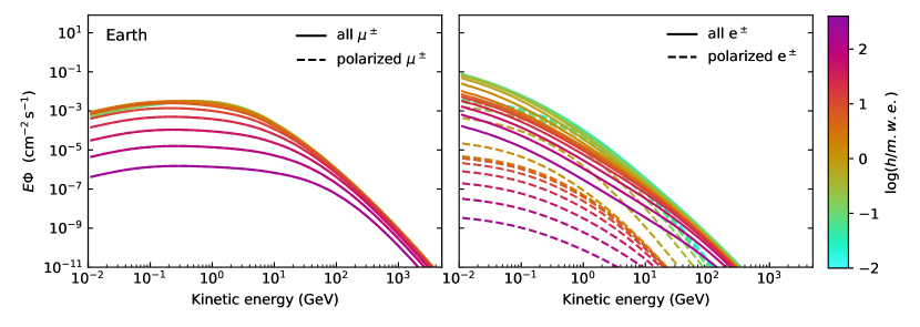
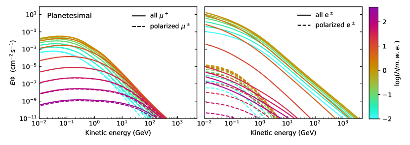
In Fig. 1, we show the underground fluxes of muons and the accompanying electrons as a function of depth (in meter water equivalent), on Earth and on a moon without an atmosphere. While the muons are highly polarized, the electron polarization is negligible. The basic reason is that electrons scatter faster than they cool (Appendix B). This implies that polarized electrons made in muon decays in the atmosphere are rapidly depolarized and do not reach the surface. Electrons produced in muon decays below the surface are also unimportant.
However, the muons cool by creating unpolarized, knock-on electrons, an unavoidable “entourage” of high energy electrons that must accompany the muons. High-energy muons () that dominate at larger depths emit photons through bremsstrahlung and initiate electromagnetic sub-cascades through . These contribute to the “entourage” of unpolarized electrons, hence diluting effects induced by the high-energy muon polarization. A given biological molecule will evolve in the presence of a spectrum of both particles. While we do not understand their separate effects, a first step is to estimate their relative densities. This is discussed more in Appendices B and C.
4 Founts
Now we have explored the effect of depolarization and dilution, we will calculate the polarized radiation doses at various environments: Mars, Titan, Venus, and bodies without an atmosphere (moons, asteroids). We are interested in founts, that we defined in the introduction as places where trans-biotic polymers can develop. The search for life in our solar system has been focused on finding water, one of the key prerequisites for life as we know it, in the form of subsurface lakes or oceans. In some environments, geologic and hydrologic activity could have enabled physical processes necessary for the growth of the first helical biopolymers (see Camprubí et al., 2019, for a review).
4.1 Worlds with a thin or negligible atmosphere
Mars is a frozen world punctuated by periods of hydrologic activity (Cabrol, 2018). Recently, a 20-km-wide lake of liquid water has been detected underneath solid ice in the Planum Australe region, at approximately 1.5 kilometer depth (Orosei et al., 2018). Although there is still no evidence for life on Mars, the red planet has once deployed environments characteristics of wet-dry cycling, a process thought to have enabled the production of the first helical biopolymers (Ross & Deamer, 2016); the Mars Exploration Rover Spirit reported 3.65-billion-year-old hot spring deposits, approximatively of the same age as the Dresser hot springs on Earth that showed evidence for microbial life (Van Kranendonk et al., 2017; Damer & Deamer, 2020). If microbial life started in similar hot springs, it is likely that after Mars’ geological death and the loss of its atmosphere, microbial life would have only be able to survive underground, since Martian subsurface seems to have the key ingredients to support life for hundreds of millions of years (Michalski et al., 2018; Checinska Sielaff & Smith, 2019).
Life on Mars could have originated when its atmosphere was much denser than today and comparable to the current Earth’s atmosphere. In consequence, the radiation dose and spectrum penetrating to the surface are likely to be quite different for Noachian and present-day Mars as discussed by Lingam et al. (2018). Mars magnetic field could have been larger in the Noachian (Mittelholz et al., 2018) but this would not affect the muon polarization (GB20). As for the possible (intermittent) variations in the cosmic ray flux, we consider them in Section 5.
Evidence has accumulated that subsurface liquid regions (lakes or oceans) exist beneath the surface of the icy moon of Jupiter, Europa, and the icy moon of Saturn, Enceladus (Thomas et al., 2016). Mass spectrometers aboard the Cassini spacecraft found that the plumes of Enceladus contain water, salts, ammonia, carbon dioxide, and small and large organic molecules, suggesting that Enceladus’ ocean may entertain an organic chemistry (Khawaja et al., 2019). In these environments, the atmosphere is negligible or absent (as in asteroids, comets or meteroids). Like on Mars, we will see that in these worlds where the atmosphere is absent, the spin-polarization transport is different than on Earth.
4.2 Worlds with a very dense atmosphere
We also consider worlds with atmospheres denser than the present Earth. Titan, Enceladus and Europa are among the most geologically active worlds in our solar system but in contrast to Enceladus and Europa, Titan possess a very dense atmosphere. The essential chemical building blocks for life are present in Titan’s atmosphere (Yung et al., 1984). Titan is also thought to have a subsurface ocean of water (Iess et al., 2012)222It is possible that major impacts on a moon like Titan, Europa or Enceladus could expel large, icy fragments with liquid, life-containing interiors (or even surface oceans) into interplanetary space. Absent a heating source, the water would soon freeze, fossilizing its contents. It is surely of long-term interest to locate, visit and examine such bodies (Dyson, 1997).. For Venus, the habitable region lies in the upper atmosphere (Morowitz & Sagan, 1967).
5 Polarized radiation doses
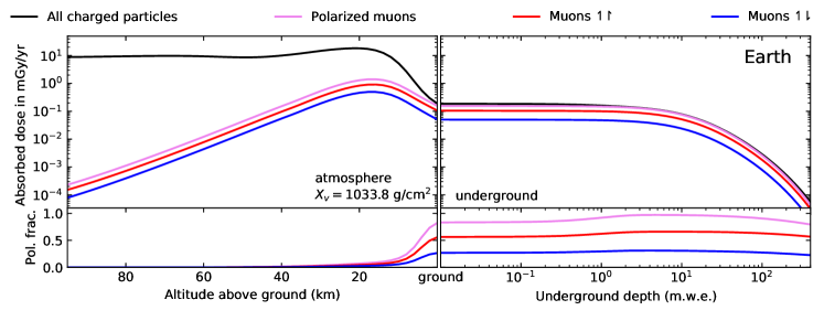
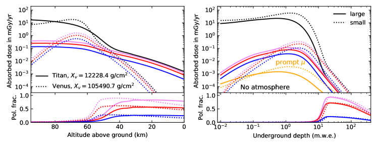
The current absorbed dose rates from cosmic radiation in different environments, are presented in Figure 2. It is an interesting coincidence that for Earth, at ground, 85% of ionizing cosmic radiation is due to the polarized muonic component that increases to almost 100% two meter water equivalent (m.w.e.) below the surface.
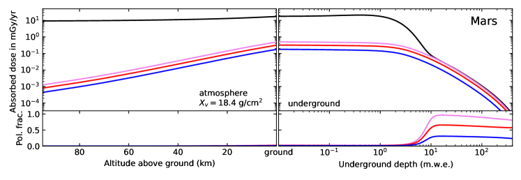
In other bodies of the solar system, the presence or absence of atmosphere leads to different results. For Mars (middle panel of Fig. 2), cosmic rays are only slightly attenuated by the thin Martian atmosphere and the polarized muons become the dominant source of cosmic radiation at m.w.e. with a dose of mGy/yr, much lower than the mGy/yr on Earth. For planetesimals without an atmosphere or smaller bodies of the solar system (bottom right panel of Fig. 2), the polarized muons component dominates at m.w.e. and with only one tenth of the intensity. In a dense, solid medium, the interaction length is much shorter than the decay length, leading predominantly to (re-)interaction of unstable hadrons rather than their decay. This suppresses the production of high energy muons and leads a swiftly decreasing polarized muon component as a function of depth.
In Titan and Venus, polarized muons dominate the radiation at altitudes , . The surface irradiation, comparable to that below of rock is negligible.
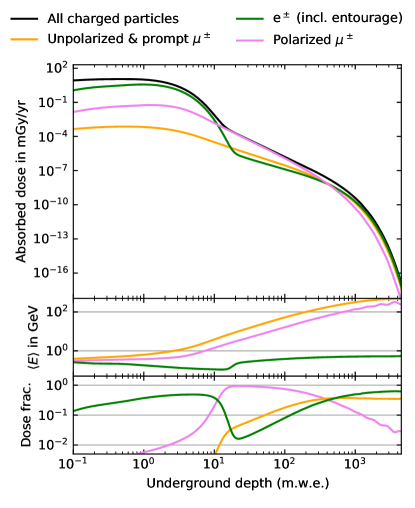
Figure 3 demonstrates that the dose deposition in a large icy body at km.w.e. depths is many orders of magnitude feebler compared to the scenarios that we study at a few m.w.e. The fraction of the polarised dose drops due to two effects: 1) kilometer depths are reached predominantly by the higher-energy, unpolarized, prompt muons (Fedynitch et al., 2019), i.e. from decays of unflavored mesons and heavy charmed hadrons, or from electromagnetic pair production; 2) the average muon energy grows because low energy muons stop or decay at shallower depths. The stopping power of high-energy muons become increasingly radiative, which deposits energy into the unpolarized electromagnetic entourage via bremsstrahlung.
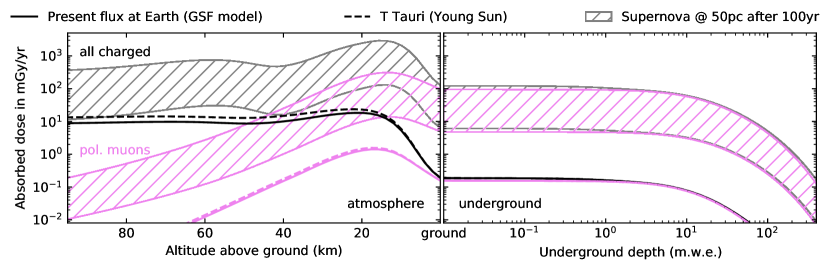
The terrestrial polarized muonic dose has a maximum of mGy/yr at the current epoch at ground level, but could have been larger during the Hadean period where a young sun could have accelerated cosmic rays beyond GeV. If the cutoff of stellar cosmic rays arises below that energy (Stellar proton events (SPEs) or a young T Tauri cosmic ray spectrum as modeled by Padovani et al. (2018), this would only change the radiation dose by a factor , as we show in Fig. 4. All environments harbor other natural sources of radiation that may exceed the dose deposited by cosmic rays. About 3.5 billion years ago, life was likely exposed to a background radiation field of mGy/yr (Karam & Leslie, 1999). However, more energetic transient events such a nearby supernova could increase the doses due to cosmic muons up to mGy/yr at ground level.We show in Fig. 4 the absorbed dose at Earth 100yrs after the explosion of a nearby supernova (Melott et al., 2017) compared to the actual doses. Since the muons retain their lodacity, higher radiation doses from cosmic muons could have altered enantioselectively the evolutionary trajectories in shorter timescales due to higher mutation rates. The closest supernova explosion over the age of the Earth was roughly pc away (e.g. Ellis & Schramm, 1995). The prompt electromagnetic (UV, X-ray, -ray) radiation could have had serious biological effects but would not be significantly chiral. By contrast, the pulse of freshly-accelerated cosmic rays is chiral and should have delivered a fluence over several thousand years, overwhelming the defenses presented by the solar wind, the magnetosphere and the atmosphere. For comparison, this is times the fluence associated with a giant, ”Carrington”-strength solar flare, albeit delivered over a much longer timescale. Activity associated with the nucleus of our Galaxy, including tidal disruption events (Pacetti et al., 2020), might also be biologically consequential. It is therefore possible, though far from assured, that life was initiated, not terminated, by such cataclysmic events.
6 Discussion
So far, scenarios for the emergence of biological homochirality involved two processes. The first one is the generation of an initial enantiomeric excess (e.e.) in biologically relevant but still simple chiral monomers, such as amino acids or sugars. Various ways to achieve an initial e.e. have been proposed: parity-violating energy differences at the molecular level (Szabó-Nagy & Keszthelyi, 1999, and references therein), asymmetric destruction due to irradiation by beta particles in radioactive decay (Vester et al., 1959), differential absorption of circularly polarized light (D’hendecourt et al., 2019), asymmetric adsorption on chiral mineral surfaces like clays (Hazen et al., 2001). Because the resulting enantiomeric excesses are very small (only up to few percent, see review by Burton & Berger, 2018), a second necessary process is the amplification of the initial e.e. from low to high values. Enantioselective chemistry might be able to amplify the e.e. up to 99.5% (Soai et al., 2000) but the validity of such chemical processes in natural environments is still debated.
In contrast, the scenario proposed by GB20 only involves enantioselective mutagenesis, for which the timescale depends on the mutation rates of the first trans-biotic polymers and the magnitude of the bias. In order for the particular enantiomeric choice observed in living systems on Earth to be causally related to the choice expressed by the weak interaction and mediated by cosmic rays, we argued in GB20 that there needs to be a coupling between the lodacity, , of the cosmic rays and the molecular chirality, , of the molecular structure. The mutation rate has to include a term proportional to the product of these two pseudoscalars. The possibilities include an electromagnetic interaction in which the scalar product of the electric and magnetic dipoles or, equivalently had a preferred sign. There is no good reason for this to occur in an isolated atom. However, it is just what is expected in a segment of a helical molecule containing a conduction or a magnetization current. In this case is negative (positive) for a right- (left-) handed helix, independent of the polarity.
We conclude with two thoughts. Firstly, Earth is the only body in the solar system with an atmosphere just the right density and scale height to ensure that muons dominate the cosmic radiation at ground level and for underground. It is thick enough to stop the other constituents, thin enough for the muons to survive. For worlds with thin or negligible atmosphere, such as Mars, polarized muons are the dominant source of cosmic radiation at depths of 10 m.w.e. while for worlds with dense atmospheres, like Venus or Titan, muons dominate below 40 km altitude but the radiation doses are negligible at the surface. Now, muons are the one constituent of cosmic radiation that is created with and retains high polarization as it decelerates to speeds when it can promote mutation of trans-biotic biopolymers. Might this be connected with the fact that Earth is the only body known to harbor life? However, we know that Mars, Venus, and Earth have undergone significant evolution. Early in the Solar system’s history, Mars probably had an atmosphere of 0.5-1 bar (Lingam et al., 2018) and Venus may have possessed an atmosphere of 1 bar until a Gyr ago or so (e.g. Way et al., 2016). However, if life originated in the early solar system, conditions could have been different from those we experience today. Therefore the special character of Earth’s atmosphere might be more relevant to life’s development than to its origin.
The second thought is that the relative importance of the muons and their electronic entourage for mutation is not understood. In GB20, ionization was taken as a proxy for mutation. If this is the case, then collisional ionization by electrons is probably more frequent than muon capture, diluting the chiral effect of the cosmic rays. Muons have advantages of better depth-dose distributions. However, even ionization may be reparable and not so conducive to genetic alteration. There could be an appreciable chiral contribution to the Hamiltonian for the formation of a muonic atom or Mu in a helical molecule. The fact that negative muons retain their polarization down to the energies where they can undergo a spin dependent capture, may also have an effect on enantioselective mutagenesis. A single muonic atom decay will produce polarized X-rays and Michel electrons333Michel electrons have a well known energy distribution with a sharp peak at 52.83 MeV and an asymmetric angular distribution if the parent muon is polarized, and would contribute to the chiral bias. and will surely fracture the molecule. Even the pickup of an electron in Mu formation could be quite disruptive. Perhaps it is muons, not electrons, that dominate mutation of trans-biotic biopolymers, thereby increasing the chiral transfer and accelerating evolution to homochirality.
These matters and the prospect of performing experimental investigations will be discussed in a future paper.
Acknowledgements
We are thankful to David Deamer, Bruce Dunham, Akimichi Taketa, for helpful discussions and encouragements. The research of NG was supported by New York University and the Simons Foundation. AF completed his work as JSPS International Research Fellow (JSPS KAKENHI Grant Number 19F19750).
References
- Akylas & Vogel (1977) Akylas, V., & Vogel, P. 1977, Hyperfine Interactions, 3, 77
- Avnir (2020) Avnir, D. 2020, New Astronomy Reviews, 101596
- Bada (1995) Bada, J. L. 1995, Nature, 374, 594
- Battistoni et al. (2015) Battistoni, G., et al. 2015, Annals Nucl. Energy, 82, 10
- Berger et al. (2017) Berger, M. J., Coursey, J., Zucker, M., & Chang, J. 2017, NIST Standard Reference Database 124 (Version 2.0.1), doi:10.18434/T4NC7P
- Burton & Berger (2018) Burton, A. S., & Berger, E. L. 2018, Life, 8, 14
- Cabrol (2018) Cabrol, N. A. 2018, The coevolution of life and environment on Mars: an ecosystem perspective on the robotic exploration of biosignatures, Mary Ann Liebert, Inc. 140 Huguenot Street, 3rd Floor New Rochelle, NY 10801 USA
- Camprubí et al. (2019) Camprubí, E., De Leeuw, J., House, C., et al. 2019, Space Science Reviews, 215, 56
- Checinska Sielaff & Smith (2019) Checinska Sielaff, A., & Smith, S. A. 2019, Geosciences, 9, 361
- Damer & Deamer (2020) Damer, B., & Deamer, D. 2020, Astrobiology, 20, 429
- Dembinski et al. (2017) Dembinski, H., Engel, R., Fedynitch, A., et al. 2017, in International Cosmic Ray Conference, Vol. 301, 35th International Cosmic Ray Conference (ICRC2017), 533
- Dermer (1986) Dermer, C. D. 1986, ApJ, 307, 47
- D’hendecourt et al. (2019) D’hendecourt, L., Modica, P., Meinert, C., Nahon, L., & Meierhenrich, U. 2019, arXiv e-prints, arXiv:1902.04575
- Dreiling & Gay (2014) Dreiling, J., & Gay, T. 2014, Physical review letters, 113, 118103
- Dyson (1997) Dyson, F. J. 1997, ATLANTIC-BOSTON-, 280, 69
- Ellis & Schramm (1995) Ellis, J., & Schramm, D. N. 1995, Proceedings of the National Academy of Sciences, 92, 235
- Fedynitch et al. (2015) Fedynitch, A., Engel, R., Gaisser, T. K., Riehn, F., & Stanev, T. 2015, in European Physical Journal Web of Conferences, Vol. 99, European Physical Journal Web of Conferences, 08001
- Fedynitch et al. (2019) Fedynitch, A., Riehn, F., Engel, R., Gaisser, T. K., & Stanev, T. 2019, Phys. Rev. D, 100, 103018
- Fulchignoni et al. (2005) Fulchignoni, M., Ferri, F., Angrilli, F., et al. 2005, Nature, 438, 785
- Gaisser et al. (2016) Gaisser, T. K., Engel, R., & Resconi, E. 2016, Cosmic Rays and Particle Physics (Cambridge University Press)
- Garwin et al. (1957) Garwin, R. L., Lederman, L. M., & Weinrich, M. 1957, Physical Review, 105, 1415
- Globus & Blandford (2020) Globus, N., & Blandford, R. D. 2020, The Astrophysical Journal, 895, L11
- Hazen et al. (2001) Hazen, R. M., Filley, T. R., & Goodfriend, G. A. 2001, Proceedings of the National Academy of Sciences, 98, 5487
- Iess et al. (2012) Iess, L., Jacobson, R. A., Ducci, M., et al. 2012, Science, 337, 457
- Karam & Leslie (1999) Karam, P. A., & Leslie, S. A. 1999, Health physics, 77, 662
- Khawaja et al. (2019) Khawaja, N., Postberg, F., Hillier, J., et al. 2019, Monthly Notices of the Royal Astronomical Society, 489, 5231
- Kulhar (2004) Kulhar, V. 2004, Pramana, 63, 543
- Lebonnois & Schubert (2017) Lebonnois, S., & Schubert, G. 2017, Nature Geoscience, 10, 473
- Lingam et al. (2018) Lingam, M., Dong, C., Fang, X., Jakosky, B. M., & Loeb, A. 2018, The Astrophysical Journal, 853, 10
- Linkin et al. (1986) Linkin, V. M., Blamont, J. E., Lipatov, A. N., et al. 1986, Soviet Astronomy Letters, 12, 40
- Lipari (1993) Lipari, P. 1993, Astroparticle Physics, 1, 195
- Meighen-Berger & Li (2019) Meighen-Berger, S., & Li, M. 2019, in International Cosmic Ray Conference, Vol. 36, 36th International Cosmic Ray Conference (ICRC2019), 961
- Melott et al. (2017) Melott, A. L., Thomas, B. C., Kachelrieß, M., Semikoz, D. V., & Overholt, A. C. 2017, ApJ, 840, 105
- Michalski et al. (2018) Michalski, J. R., Onstott, T. C., Mojzsis, S. J., et al. 2018, Nature Geoscience, 11, 21
- Mittelholz et al. (2018) Mittelholz, A., Morschhauser, A., Johnson, C. L., et al. 2018, Earth and Space Science, 5, 410
- Morowitz & Sagan (1967) Morowitz, H., & Sagan, C. 1967, Nature, 215, 1259
- Naaman & Waldeck (2012) Naaman, R., & Waldeck, D. H. 2012, The journal of physical chemistry letters, 3, 2178
- Nagamine (2003) Nagamine, K. 2003, Introductory muon science (Cambridge University Press)
- Nanda et al. (2007) Nanda, V., Andrianarijaona, A., & Narayanan, C. 2007, Protein science, 16, 1667
- Orosei et al. (2018) Orosei, R., Lauro, S., Pettinelli, E., et al. 2018, Science, 361, 490
- Pacetti et al. (2020) Pacetti, E., Balbi, A., Lingam, M., Tombesi, F., & Perlman, E. 2020, Monthly Notices of the Royal Astronomical Society, 498, 3153
- Padovani et al. (2018) Padovani, M., Ivlev, A. V., Galli, D., & Caselli, P. 2018, A&A, 614, A111
- Particle Data Group (2020) Particle Data Group. 2020, Progress of Theoretical and Experimental Physics, 2020, 083C01
- Pizzarello (2006) Pizzarello, S. 2006, Accounts of Chemical Research, 39, 231
- Roesler et al. (2001) Roesler, S., Engel, R., & Ranft, J. 2001, The Monte Carlo Event Generator DPMJET-III, 1033
- Rosenberg (2019) Rosenberg, R. A. 2019, Symmetry, 11, 528
- Ross & Deamer (2016) Ross, D. S., & Deamer, D. 2016, Life, 6, 28
- Soai et al. (2000) Soai, K., Shibata, T., & Sato, I. 2000, Accounts of Chemical Research, 33, 382
- Standard Atmosphere (1976) Standard Atmosphere, U. S. 1976, US Gov. Print. Off., Washington, DC
- Szabó-Nagy & Keszthelyi (1999) Szabó-Nagy, A., & Keszthelyi, L. 1999, Proceedings of the National Academy of Sciences, 96, 4252
- Thomas et al. (2016) Thomas, P., Tajeddine, R., Tiscareno, M., et al. 2016, Icarus, 264, 37
- Totsingan et al. (2012) Totsingan, F., Jain, V., & Green, M. M. 2012, Artificial Dna: Pna & Xna, 3, 31
- Van Kranendonk et al. (2017) Van Kranendonk, M. J., Deamer, D. W., & Djokic, T. 2017, Scientific American, 317, 28
- Vester et al. (1959) Vester, F., Ulbricht, T., & Krauch, H. 1959, Naturwissenschaften, 46, 68
- Volkova & Zatsepin (1965) Volkova, L. V., & Zatsepin, G. T. 1965, in International Cosmic Ray Conference, Vol. 1, International Cosmic Ray Conference, 1039
- Way et al. (2016) Way, M. J., Del Genio, A. D., Kiang, N. Y., et al. 2016, Geophysical Research Letters, 43, 8376
- Yung et al. (1984) Yung, Y. L., Allen, M., & Pinto, J. P. 1984, Astrophysical Journal Supplement Series, 55, 465
Appendix A Scattering and ionization loss
The rate of loss of kinetic energy by a cosmic ray in an environment where the molecular density is , is dominated by the ionization of electrons and can be approximated by
| (A1) |
where is the speed, the sum is over all the atomic numbers of the nuclei in the molecule and is the ratio of the maximum to the minimum impact parameter given roughly by , where is the momentum and is a mean ionization potential. As the energy loss is dominated by distant encounters, the energy fluctuations are small and the kinetic energy can be regarded as function of time.
Nuclear recoils do not contribute to the stopping power but they dominate the scattering. Consider a cosmic ray with momentum p making an angle with the direction of its magnetic moment, which we can regard as fixed in space. The mean square rate of change of the transverse momentum by nuclear and electron collisions can be similarly expressed as
| (A2) |
Now, the lodacity, , and if we average over azimuth in the scattering, we find that . Again the fluctuations will be small and can be ignored.
It is helpful to introduce a quantity
| (A3) |
which we call the “lethargy” for a cosmic ray with rest mass . We can then combine these three equations to obtain
| (A4) |
and so, , where is the depolarization factor. For cosmic ray muons, electrons in water, .
Appendix B Knock-on electrons from cosmic ray muons under water
Consider, as a specific example, muons incident upon the surface of the ocean on Earth. We have argued that muons decelerate through ionization loss while retaining most of their initial lodacity. For the energies that dominate the particle flux at the surface of the earth, , they stop at a depth of tens of meters before they decay. When they become non-relativistic, their range scales . After they cool, they will be captured on atoms, (), or capture an electron, (). By contrast, electrons scatter before they decelerate. Polarized electrons created through muon decay are rapidly depolarized and are unimportant compared with the knock-on electrons which will cool and thermalize on the spot by creating more knock-on electrons, forming an unpolarized “entourage”, accompanying the muons.
The polarized muons and the unpolarized electrons will compete in creating mutations of trans-biotic molecules, diluting the chiral transfer. In order to quantify this effect, we first consider a fixed number density high energy muons crossing a volume that is large enough to allow the knock-on electrons to cool locally and small enough for the muons not to cool in traversing it. Introduce a conserved number current in energy space of high energy muons , the number of particles cooling through a kinetic energy per unit volume and time. Let this be established at some moderately relativistic energy . Next, approximate the rate per unit volume, , at which a muon, with kinetic energy , produces electrons with kinetic energy lying in . Now, c.f. Eq. (1). Likewise we introduce the current of electrons in energy space , with . satisfies
| (B1) |
Next multiply Eq. B1 by and integrate over . We find the approximate solution
| (B2) |
In other words, the knock-on electron energy current in energy space at low energy is roughly the same as the energy current for the muons at high energy.
In this paper we are most interested in the muon and electrons spectra which can then contribute to the biological evolution of trans-biotic polymers and introduce a chiral bias. Many processes contribute to the full picture as we shall discuss elsewhere. For the moment, as an example, let us consider electrons which are known to induce mutation in DNA. These are produced by muons with energy . As the energy current in muons with energy is roughly the same as the energy flowing through as electrons, we can conclude that the number current of electrons is roughly times the conserved number current of muons. The implications of this for biological processes then depend on combining these rates with the relevant cross-sections.
Appendix C Computation of particle fluxes
We compute differential particle fluxes , where is the kinetic energy and is the slant depth in g/cm2, using the one-dimensional cascade equation solver MCEq444https://github.com/afedynitch/MCEq (Version 1.3) (Fedynitch et al., 2015) that is optimized for calculations of inclusive atmospheric lepton fluxes at high energies above a few GeV (Fedynitch et al., 2019). We have extend the kinetic energy range down to 10 MeV and for computations in different media, such as carbon-dioxide and water by using hadronic cross sections and particle production tables from the DPMJET-III-19.1555https://github.com/afedynitch/DPMJET event generator (Roesler et al., 2001). Electromagnetic cross sections have been computed using the numerical routines from Meighen-Berger & Li (2019). Ionization losses are based on tables from (Particle Data Group, 2020; Berger et al., 2017) and are tracked for each charged particle whereas energy deposition by tertiary electromagnetic cascades from fast neutrons are neglected. MCEq adapts the notation and formulae for muon polarization in the relativistic approximation from Lipari (1993) that we verified to be valid for MeV.
The flux of cosmic rays in the solar system is considered to be isotropic and represented by the Global Spline Fit (GSF) (Dembinski et al., 2017), which is an modern parameterization of cosmic ray fluxes at Earth between rigidity of a few GV and the highest observed energies at Earth. The rigidity cutoff due to the planetary magnetic field, the location within the solar system and the Sun’s level of activity affects the low energy cosmic rays below a few GV/nucleon. The omission of magnetic fields and solar modulation is considered as a source of uncertainty of this calculation but is not expected to qualitatively change the result, in particular not at larger depths or underground.
The absorbed dose rate in Gy/s is calculated from the differential fluxes with the default units (GeV cm2 s sr)-1 using
where , the altitude above ground and the radius of the planet. The index iterates over particle species. The expression for takes into account that at higher altitudes, particle cascades can develop upwards relative to the horizon.
The models of the planetary atmospheres are the Standard Atmosphere (1976) for Earth, derived from Huygens Atmospheric Structure Instrument measurements for Titan (Fulchignoni et al., 2005), from the Soviet VeGa-2 probe (Linkin et al., 1986; Lebonnois & Schubert, 2017) for Venus, and from a fit of piece-wise barometric formulae to Mars Global Surveyor data Underground fluxes are computed for a water target with the ionization loss computed computed with ESTAR and PSTAR (Berger et al., 2017). Within the precision of this calculation and depths km, the difference in stopping power compared to a dedicated calculation in standard rock is negligible for muons.
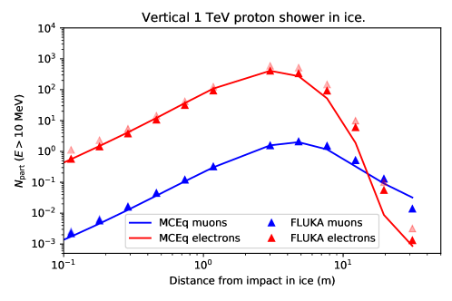
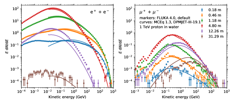
In Figs. 5 and 6 MCEq is compared with FLUKA 4.0666https://fluka.cern (Battistoni et al., 2015) simulations in water for 1 TeV proton projectiles. The technical low energy cutoff in MCEq is 10 MeV, which is sufficient to capture a good description for the total number of muons (blue curve in Fig. 5 and right panel of Fig. 6). At tens of meters in depth, the differences between codes become more pronounced since the particle cascade is increasingly affected by multiple subsequent interactions that amplify differences in production and absorption cross sections between the models. To simulate water targets with MCEq it was necessary to include ionization losses for all charged particles and obtain inelastic cross sections for water from the hadronic interaction models. None the less the agreement is remarkably good since MCEq has not yet been employed for simulations down to low energies and water targets. For electrons, simulated using MCEq and electromagnetic cross sections from Meighen-Berger & Li (2019), the agreement is good except at around the cascade maximum. Since the majority of electromagnetic energy is of hadronic origin through the process, the hadronic model differences between DPMJET-III-19.1 and PEANUT/FLUKA have impact. An estimate for the fraction of electrons that are lost due to the 10 MeV cutoff in MCEq can be made from the comparison between the pale and dark red triangles in Fig. 5. Since the gradient of the electromagnetic component is very steep after the maximum, the differences between MCEq and FLUKA do not qualitatively alter our conclusions from the main text with respect to the depth at which polarized muons constitute the dominant source of cosmic radiation.
