Domain Adaptation for the Segmentation of Confidential Medical Images

Abstract

Convolutional neural networks (CNNs) have led to significant improvements in the semantic segmentation of images. When source and target datasets come from different modalities, CNN performance suffers due to domain shift. In such cases data annotation in the target domain becomes necessary to maintain model performance. To circumvent the re-annotation process, unsupervised domain adaptation (UDA) is proposed to adapt a model to new modalities using solely unlabeled target data. Common UDA algorithms require access to source domain data during adaptation, which may not be feasible in medical imaging due to data sharing restrictions. In this work, we develop an algorithm for UDA where the source domain data is inaccessible during target adaptation. Our approach is based on encoding the source domain information into an internal distribution that is used to guide adaptation in the absence of source samples. We demonstrate the effectiveness of our algorithm by comparing it to state-of-the-art medical image semantic segmentation approaches on two medical image semantic segmentation datasets.

1 Introduction

Employing CNNs in semantic segmentation tasks has been proven to be extremely helpful in various applications, including object tracking [Yilmaz et al.(2006)Yilmaz, Javed, and Shah, Bertinetto et al.(2016)Bertinetto, Valmadre, Henriques, Vedaldi, and Torr, Zhu et al.(2018)Zhu, Yang, Liu, Kim, Zhang, and Yang], self-driving cars [Kim and Canny(2017), Hecker et al.(2018)Hecker, Dai, and Van Gool], and medical image analysis [Ker et al.(2018)Ker, Wang, Rao, and Lim, Shen et al.(2017)Shen, Wu, and Suk, Ayache(2017), Kazeminia et al.(2020)Kazeminia, Baur, Kuijper, van Ginneken, Navab, Albarqouni, and Mukhopadhyay]. This success, however, is conditioned on the availability of huge manually annotated datasets to supervise the training of state-of-the-art (SOTA) network structures [Rostami et al.(2018)Rostami, Huber, and Lu, Toldo et al.(2020)Toldo, Maracani, Michieli, and Zanuttigh]. This condition is not always realized in practice, especially in fields such as medical image segmentation, where annotating data requires the input of trained experts and privacy regulations make sharing data for crowd-sourcing extremely restricted, and at times impossible. A characteristic of data in the area of medical image segmentation is the existence of domain shift between different imaging modalities, which stems from using imaging devices based on totally different electromagnetic principles, e.g., CT vs MRI. When domain gap exists between the distributions of the training (source) and the testing (target) data, the performance of CNNs can degrade significantly. This makes continual data annotation necessary for maintaining model performance.

Domain shift is a major area of concern, as data annotation is a challenging procedure even for the simplest semantic segmentation tasks [Liu et al.(2011)Liu, Xiong, Pulli, and Shapiro]. Annotating medical images is also expensive, as annotation can be performed only by physicians, who undergo years of training to obtain domain expertise. Unsupervised domain adaptation (UDA) is a learning setting aimed at reducing domain gap without data annotation in the target domain. The goal is to adapt a source-trained model for improved generalization in the target domain using solely unannotated data [Ghifary et al.(2016)Ghifary, Kleijn, Zhang, Balduzzi, and Li, Venkateswara et al.(2017)Venkateswara, Eusebio, Chakraborty, and Panchanathan, Saito et al.(2018)Saito, Watanabe, Ushiku, and Harada, Zhang et al.(2018b)Zhang, Ouyang, Li, and Xu]. The core idea in UDA is to achieve knowledge transfer from the source domain to the target domain by aligning the latent features of the two domains in an embedding space. This idea has been implemented either using adversarial learning [Hoffman et al.(2018)Hoffman, Tzeng, Park, Zhu, Isola, Saenko, Efros, and Darrell, Dou et al.(2019)Dou, Ouyang, Chen, Chen, Glocker, Zhuang, and Heng, Tzeng et al.(2017)Tzeng, Hoffman, Saenko, and Darrell, Bousmalis et al.(2017)Bousmalis, Silberman, Dohan, Erhan, and Krishnan], directly minimizing the distance of distributions of the latent features with respect to a probability metric [Chen et al.(2019a)Chen, Xie, Huang, Rong, Ding, Huang, Xu, and Huang, Sun et al.(2017a)Sun, Feng, and Saenko, Lee et al.(2019)Lee, Batra, Baig, and Ulbricht, Rostami(2022)], or a combination of the two [Choi et al.(2019)Choi, Kim, and Kim, Sankaranarayanan et al.(2018)Sankaranarayanan, Balaji, Castillo, and Chellappa].

While existing UDA algorithms have been successful in reducing cross-domain gap, the vast majority of these approaches require sharing data between the source and target domains to enforce distribution alignment. This requirement limits the applicability of most existing works when sharing data may not be possible, e.g., sharing data is heavily regulated in healthcare domains due to the confidentiality of patient data and from security concerns. Until recently, there has been little exploration of UDA when access to the source domain is limited [Kundu et al.(2020)Kundu, Venkat, Babu, et al., Saltori et al.(2020)Saltori, Lathuiliére, Sebe, Ricci, and Galasso, Qiu et al.(2021)Qiu, Zhang, Lin, Niu, Liu, Du, and Tan, Yang et al.(2021)Yang, Wang, van de Weijer, Herranz, and Jui, Rostami and Galstyan(2021)]. These recent works benefit from generative adversarial learning to maintain source distribution information. However, addressing UDA for classification tasks limits the applicability of such methods to the problem of organ semantic segmentation [Zhao et al.(2019)Zhao, Li, Wan, Sekuboyina, Hu, Tetteh, Piraud, and Menze]. A similar problem is encountered with UDA for street semantic segmentation [Kundu et al.(2021)Kundu, Kulkarni, Singh, Jampani, and Babu], given medical devices produce data distributions requiring additional preparation with large background areas [Zhou et al.(2019)Zhou, Li, Bai, Wang, Chen, Han, Fishman, and Yuille]. Recent medical works propose adaptation without source access via entropy minimization  [Bateson et al.(2022)Bateson, Kervadec, Dolz, Lombaert, and Ayed, Bateson et al.(2020)Bateson, Kervadec, Dolz, Lombaert, and Ben Ayed], but these methods are susceptible to degenerate solutions.

Contribution: we develop a UDA algorithm for the semantic segmentation of medical images when sharing data is infeasible due to confidentiality or security concerns. Our approach is able to reduce domain gap without having direct access to the source data during adaptation. We learn the internal distribution for the source domain, and transfer knowledge between the source and target domains by distribution alignment between the learned internal distribution and the latent distribution of features of the target domain. We validate our algorithm on two medical image segmentation datasets, and observe comparable performance to SOTA methods based on joint training.

2 Related Work

SOTA semantic segmentation algorithms use deep neural network architectures to exploit large annotated datasets [Long et al.(2015)Long, Shelhamer, and Darrell, Noh et al.(2015)Noh, Hong, and Han, Lin et al.(2017)Lin, Milan, Shen, and Reid, LeCun et al.(2015)LeCun, Bengio, and Hinton]. These approaches are based on training a CNN encoder using manually annotated segmentation maps to learn a latent embedding of the data. An up-sampling decoder combined with a classifier is then used to infer pixel-wise estimations for the true semantic labels. Performance of such methods is high when large amounts of annotated data are available for supervised training. However, these methods are not suitable when the goal is to transfer knowledge between different domains [Saito et al.(2018)Saito, Watanabe, Ushiku, and Harada, Pan et al.(2019)Pan, Yao, Li, Wang, Ngo, and Mei]. Model adaptation from a fully annotated source domains to a target domains has been explored in both semi-supervised and unsupervised settings. Semi-supervised approaches rely on the presence of a small number of annotated target data samples [Motiian et al.(2017)Motiian, Jones, Iranmanesh, and Doretto, Zhang et al.(2019)Zhang, Chen, Huang, Lin, and Zhang]. For example, a weakly supervised signal on the target domain can be obtained using bounding boxes. However, manual data annotation of a small number of images is still a considerable bottleneck in the area of medical imaging because only trained professionals can perform this task. For this reason, UDA algorithms are more appealing for healthcare applications.

UDA approaches have explored two main strategies to reduce the domain gap. A large number of works rely on generative adversarial networks (GANs) [Zhang et al.(2018a)Zhang, Ouyang, Li, and Xu, Kamnitsas et al.(2017a)Kamnitsas, Baumgartner, Ledig, Newcombe, Simpson, Kane, Menon, Nori, Criminisi, Rueckert, and Glocker]. The core idea is to use a GAN loss such that data points from both domains can be mapped into a domain-invariant embedding space [Hoffman et al.(2018)Hoffman, Tzeng, Park, Zhu, Isola, Saenko, Efros, and Darrell]. To this end, a cross-domain discriminator network is trained to classify whether data embeddings correspond to the source or target domain. An encoder network attempts to fool the discriminator by producing domain agnostic representations for source and target data points. Following this alternating optimization process, a classifier trained using source domain encodings produced by the encoder network would also generalize in the target domain [Ma et al.(2019)Ma, Zhang, and Xu, Dou et al.(2018)Dou, Ouyang, Chen, Chen, and Heng]. The weakness of GANs is mode collapse, which requires careful fine-tuning and selection of hyper-parameters in order to be overcome.

Other UDA approaches aim to directly align the distributions of the two domains in a shared embedding space [Lee et al.(2019)Lee, Batra, Baig, and Ulbricht, Rostami(2021b), Stan and Rostami(2021)]. A shared encoder network is used to generate latent features for both domains. A common latent feature space is achieved by minimizing a suitable probability distance metric between the source and target embeddings [Drossos et al.(2019)Drossos, Magron, and Virtanen, Le et al.(2019)Le, Habrard, and Sebban, Rostami et al.(2019)Rostami, Kolouri, Eaton, and Kim, Liu et al.(2020)Liu, Zhang, Song, Zhang, O’Donnell, Huang, Chen, and Cai]. Selecting proper distance metrics has been the major focus of research for these approaches. Optimal transport has been found particularly suitable for deep learning based UDA  [Courty et al.(2016)Courty, Flamary, Tuia, and Rakotomamonjy]. We utilize the Sliced Wasserstein Distance (SWD) [Lee et al.(2019)Lee, Batra, Baig, and Ulbricht, Rostami(2021a)] variant of the optimal transport with similar properties, but which allows for fast gradient based optimization.

The above mentioned sets of approaches have been found helpful in various medical semantic segmentation applications [Huo et al.(2018)Huo, Xu, Bao, Assad, Abramson, and Landman, Zhang et al.(2018c)Zhang, Miao, Mansi, and Liao, Chen et al.(2018)Chen, Dou, Chen, and Heng, Kamnitsas et al.(2017b)Kamnitsas, Baumgartner, Ledig, Newcombe, Simpson, Kane, Menon, Nori, Criminisi, Rueckert, et al.]. However, both strategies require direct access to source domain data for computing the loss functions. To relax this requirement, UDA has been recently explored in a source-free setting to address scenarios where the source domain is not directly accessible [Kundu et al.(2020)Kundu, Venkat, Babu, et al., Saltori et al.(2020)Saltori, Lathuiliére, Sebe, Ricci, and Galasso]. Both Kundu et al. [Kundu et al.(2020)Kundu, Venkat, Babu, et al.] and Saltori et al. [Saltori et al.(2020)Saltori, Lathuiliére, Sebe, Ricci, and Galasso] target image classification, and benefit from generative adversarial learning to generate pseudo-data points that are similar to the source domain data in the absence of actual source samples. While both approaches are suitable for classification problems, extending them to semantic segmentation of medical images is not trivial. First, training models that can generate realistic medical images is considerably more challenging due to importance of fine details. Second, one may argue that if generated images are too similar to real images, the information confidentiality of patients in the training data may still be compromised. Our work is based on using a dramatically different approach. We develop a source-free UDA algorithm that performs the distribution alignment of two domains in an embedding space by using an intermediate internal distribution to relax the need for source data.

3 Problem Formulation

Figure 1: Proposed method: We first perform supervised training on source MR images. Using the source embeddings we characterize an internal distribution via a GMM distribution in the latent space. We then perform source free adaptation by matching the embedding of the target CT images to the learnt GMM distribution, and fine tuning of the classifier on GMM samples. Finally, we verify the improved performance that our model gains from model adaptation.

Consider a source domain $D^{S}=(X^{S},Y^{S})$ with annotated data and a target domain $D^{T}=(X^{T})$ with unannotated data that despite having different input spaces $X^{S}$ and $X^{T}$, e.g., due to using different medical imaging techniques, share the same segmentation map space $Y$, e.g., the same tissue/organ classes. Following the standard UDA pipeline, the goal is to learn a segmentation mapping function for the target domain by transferring knowledge from the source domain. To this end, we must learn a function $f_{\theta}(\cdot):\{X^{S}\cup X^{T}\}\rightarrow\{Y\}$ with learnable parameters $\theta$, e.g., a deep neural network, such that given an input image $x^{*}$, the function returns a segmentation mask $\hat{y}$ that best approximates the ground truth segmentation mask $y^{*}$. Given the annotated training dataset $\{(x^{s},y^{s})\}_{i=1}^{N}$ in the source domain, it is straightforward to train a segmentation model that generalizes well in the source domain through solving an empirical risk minimization (ERM) problem, i.e., $\hat{\theta}=\arg\min_{\theta}\frac{1}{N}\sum_{i=1}^{N}\mathcal{L}(y^{s},f_{\theta}(x^{s})))$, where $\mathcal{L}$ is a proper loss function, e.g., the pixel-wise cross-entropy loss, defined as $\mathcal{L}_{ce}(y^{*},\hat{y})=-\sum_{i=1}^{W}\sum_{j=1}^{H}\sum_{k=1}^{K}y^{*}_{ijk}\log\hat{y}_{ijk}$. Here, $K$ denotes the number of segmentation classes, and $W,H$ represent the width and the height the input images, respectively. Each pixel label $y^{*}_{ij}$ will be represented as a one hot vector of size $K$ and $\hat{y}_{ij}$ is the prediction vector which assigns a probability weight to each label. Due to the existence of domain gap across the two domains, i.e. discrepancy between the source domain distribution $p^{s}(X)$ and the target domain distribution $p^{t}(X)$, the source-trained model using ERM may generalize poorly in the target domain. We want to benefit from the information encoded in the target domain unannotated dataset $\{x^{t}\}_{i=1}^{M}$ to improve the model generalization in the target domain further.

We follow the common strategy of domain alignment in a shared embedding space to adress UDA. Consider our model $f$ to be a deep convolutional neural network (CNN). Let $f=\phi\circ\chi\circ\psi$, where $\psi(\cdot):\mathbb{R}^{W\times H\times C}\rightarrow\mathbb{R}^{U\times V}$ is a CNN encoder, $\chi(\cdot):\mathbb{R}^{U\times V}\rightarrow\mathbb{R}^{W\times H\times K}$ is an up-scaling CNN decoder, and $\phi(\cdot):\mathbb{R}^{W\times H\times K}\rightarrow\mathbb{R}^{W\times H\times K}$ is a classification network that takes as inputs latent space representations and assigns label-probability values. We model the shared embedding space as the output space of the sub-network $\chi\circ\psi(\cdot)$. Solving UDA reduces to ensuring the source and target embedding distributions are aligned in the embedding space. This translates into minimizing the distributional discrepancy between the $\chi\circ\psi(p^{s}(\cdot))$ and $\chi\circ\psi(p^{t}(\cdot))$ distributions. A large group of UDA algorithms [Wu et al.(2018)Wu, Han, Lin, Uzunbas, Goldstein, Lim, and Davis, Zhang et al.(2017)Zhang, David, and Gong] select a probability distribution metric $D(\cdot,\cdot)$, e.g. SWD or KL-divergence, and then use the source and the target domain data points, $X^{S}=[x^{s}_{1},\ldots,x^{s}_{N}]$ and $X^{T}=[x^{t}_{1},\ldots,x^{t}_{N}]$, to minimize the loss term $D(\chi\circ\psi(p^{s}(\cdot)),\chi\circ\psi(p^{t}(\cdot)))$ as a regularizer. However, this will constrain the user to have access to the source domain data to compute $D(\chi\circ\psi(p^{s}(\cdot)),\chi\circ\psi(p^{t}(\cdot)))$ that couples the two domains. We provide a solution to align the two domains without sharing the source domain data, that benefits from an intermediate probability distribution.

4 Proposed Algorithm

Our proposed approach is based on using the internal distribution $\mathcal{P_{Z}}$ as a surrogate for the learned distribution of the source domain in the embedding space. Upon training $f_{\theta}$ using ERM, the embedding space would become discriminative for the source domain. This means that the source distribution in the embedding space will be a multimodal distribution, where each mode denotes one of the classes. This distribution can be modeled as a Gaussian Mixture Model (GMM). To develop a source-free UDA algorithm, we can draw random samples from the GMM and instead of relying on the source data, align the target domain distribution with the internal distribution in the embedding space. In other words, we estimate the term $D(\chi\circ\psi(p^{s}(\cdot)),\chi\circ\psi(p^{t}(\cdot)))$ with $D(\mathcal{P_{Z}}(\cdot),\chi\circ\psi(p^{t}(\cdot)))$ which does not depend on source samples. We use SWD as the distribution metric for minimizing the domain discrepancy. A visual concept-level description for our approach is presented in Figure 1.

The intermediate distribution. The function $\psi\circ\chi$ transforms the input distribution $p^{s}(\cdot)$ to the internal distribution $\mathcal{P_{Z}}(\cdot)=\chi\circ\psi(p^{s}(\cdot))$ based on which the classifier $\phi$ assigns labels. This distribution will have $K$ modes. Our idea is to approximate $\mathcal{P_{Z}}(\cdot)$ via a GMM with $\omega\times K$ components, with $\omega$ components for each of the $K$ semantic classes:

$$\small\mathcal{P_{Z}}(z)=\sum_{c=1}^{\omega K}\alpha_{c}p_{c}(z)=\sum_{c=1}^{\omega K}\alpha_{c}\mathcal{N}(z|\mu_{c},\Sigma_{c}),$$

where $\alpha_{c}$ represents the mixture probabilities, $\mu_{c}$ represents the mean of the Gaussian $c$, and $\Sigma_{c}$ is the covariance matrix of the $c^{th}$ component. Under the above representation, each semantic class $k\in\{1\dots K\}$ will be represented by $\omega$ components: $(k-1)\omega+1\dots k\omega$. When the network $f$ is trained on the source domain, we can estimate the GMM parameters class-conditionally from the latent features obtained from the source training samples $\{\phi(\chi(x^{s}))_{ijt},y^{s}_{ij}\}$. Once class specific latent embeddings are computed via access to the labels $Y^{S}$, we estimate the corresponding $\omega$ components using the EM algorithm.

Sample selection. To improve class separations in the internal distribution $\mathcal{P}_{Z}$, we only use high-confidence samples in each class for estimating parameters of $p_{c}(\cdot)$. We use a confidence threshold parameter $\rho$, and discard all samples for which the classifier confidence on its prediction $p_{ij}$ is strictly less than $\rho$. This step helps cancel out class outliers. Let $\mathcal{S}_{\rho}=\{(x_{ij}^{s},y_{ij}^{s})|\max\phi(\chi(\psi(x_{ij})))>\rho\}$ be the source data pixels on which the classifier $\phi$ assigns confidence greater than $\rho$. Also, let $\mathcal{S}_{\rho,k}=\{(x,y)|(x,y)\in\mathcal{S}_{\rho},y=k\}$. Then, for each class $k$ we generate empirical estimates for the $\omega$ components defined by triplets $(\hat{\alpha}_{\omega(k-1)+1},\hat{\mu}_{\omega(k-1)+1},\hat{\Sigma}_{\omega(k-1)+1})\dots(\hat{\alpha}_{\omega k},\hat{\mu}_{\omega k},\hat{\Sigma}_{\omega k})$ by applying EM to $\mathcal{S}_{\rho,k}$ data points.

The adaptation loss. Given the estimated internal distribution parameters $\hat{\alpha},\hat{\mu},\hat{\Sigma}$, we can perform domain alignment. Adapting the model should lead to the target latent distribution $\chi(\psi(p^{t}(X)))$ matching the distribution $\mathcal{P}_{Z}$ in the embedding space. To this end, we can generate a pseudo-dataset $D^{P}=(Z^{P},Y^{P})$ by drawing samples from the GMM and aligning $\chi(\psi(X^{T}))$ with $Z^{P}$ to reduce the domain gap. The alignment loss can then be formalized as:

$$\small\begin{split}\mathcal{L}_{adapt}=\mathcal{L}_{ce}(\phi(Z^{P}),Y^{P})+\lambda\mathcal{D}(\chi(\psi(X^{T})),Z^{P})\end{split}$$ (1)

The first term in Eq. 1 involves fine-tuning the classifier on samples from the pseudo-dataset $(Z^{P},Y^{P})$ to ensure that it would continue to generalize well. The second term enforces the distributional alignment. Since the source samples are not used in Eq. 1, data confidentiality will also be preserved. The last ingredient for our approach is selection of the distance metric $\mathcal{D}(\cdot,\cdot)$. We used SWD for this purpose. The pseudocode for our approach, called Source Free semantic Segmentation (SFS), is presented in Alg.  1.

Algorithm 1 $\mathrm{SFS}\left(\lambda,\rho,\omega\right)$

1:Initial Training:

2:  Input: Source dataset $\mathcal{D}^{\mathcal{S}}=(\bm{X}^{\mathcal{S}},\bm{Y}^{\mathcal{S}})$,

3:    Training on Source Domain:

4:     $\hat{\theta}_{0}=\arg\min_{\theta}\sum_{i}\mathcal{L}(f_{\theta}(\bm{x}_{i}^{s}),\bm{y}_{i}^{s})$

5:   Internal Distribution Estimation:

6:     Set $\rho=.97$, compute $\mathcal{S}_{\rho,k}$, and estimate $\hat{\alpha}_{j},\hat{\mu}_{j},$ and $\hat{\Sigma}_{j}$ class conditionally via EM

7:Model Adaptation:

8:   Input: Target dataset $\mathcal{D}^{\mathcal{T}}=(\bm{X}^{\mathcal{T}})$

9:   Pseudo-Dataset Generation:

10:$\mathcal{D}^{\mathcal{P}}=(\textbf{Z}^{\mathcal{P}},\textbf{Y}^{\mathcal{P}})=([\bm{z}_{1}^{p},\ldots,\bm{z}_{N}^{p}],[\bm{y}_{1}^{p},\ldots,\bm{y}_{N}^{p}])$, where: $\bm{z}_{i}^{p}\sim\mathcal{P}_{Z}(\bm{z}),1\leq i\leq N_{p}$

11:   for $itr=1\rightarrow ITR$ do

12:     Draw batches from $\mathcal{D}^{\mathcal{T}}$ and $\mathcal{D}^{\mathcal{P}}$

13:     Update the model by solving Eq. (1)

14:   end for

5 Experimental Validation

5.1 Datasets

Multi-Modality Whole Heart Segmentation Dataset (MMWHS) [Zhuang and Shen(2016)]: this dataset consists of multi-modality whole heart images obtained on different imaging devices at different imaging sites. Segmentation maps are provided for $20$ MRI 3D heart images and $20$ CT 3D heart images which have domain gap. Following the UDA setup, we use the MRI images as the source domain and CT images as the target domain. We perform UDA with respect to four of the available segmentation classes: ascending aorta (AA), left ventricle blood cavity (LVC), left atrium blood cavity (LAC), myocardium of the left ventricle (MYO).

We will use the same experimental setup and parsed dataset used by Dou et al. [Dou et al.(2018)Dou, Ouyang, Chen, Chen, and Heng] for fair comparison. For the MRI source domain we use augmented samples from $16$ MRI 3D instances. The target domain consists of augmented samples from of $14$ 3D CT images, and we report results on $4$ CT instances, as proposed by Chen et al. [Chen et al.(2020)Chen, Dou, Chen, Qin, and Heng]. Each 3D segmentation map used for assessing test performance is normalized to have zero mean and unit variance.

CHAOS MR $\rightarrow$ Multi-Atlas Labeling Beyond the Cranial Vault: the second domain adaptation task consists of data frames from two different dataset. As source domain we, consider the the 2019 CHAOS MR dataset [Kavur et al.(2019)Kavur, Selver, Dicle, Barıs, and Gezer], previously used in the 2019 CHAOS Grad Challenge. The dataset consists of both MR and CT scans with segmentation maps for the following abdominal organs: liver, right kidney, left kidney and spleen. Similar to [Chen et al.(2020)Chen, Dou, Chen, Qin, and Heng] we use the T2-SPIR MR images as the source domain. Each scan is centered to zero mean and unit variance, and values more than three standard deviations away from the mean are clipped. In total, we obtain $20$ MR scans, $16$ of which we use for training and $4$ for validation. The target domain is represented by the dataset which was presented in the Multi-Atlas Labeling Beyond the Cranial Vault MICCAI 2015 Challenge [Landman et al.(2015)Landman, Xu, Igelsias, Styner, Langerak, and Klein]. We utilize the $30$ CT scans in the training set which are provided segmentation maps, and use $24$ for adaptation and $6$ for evaluating generalization performance. The value range in the CT scans was first clipped to $[-125,275]$ HU following literature [Zhou et al.(2019)Zhou, Li, Bai, Wang, Chen, Han, Fishman, and Yuille]. The images were re-sampled to an axial view size of $256\times 256$. Background was then cropped such that the distance between any labeled pixel and the image borders is at least $30$ pixels, and scans were again resized to $256\times 256$. Finally, each 3D scan was normalized independently to zero mean and unit variance, and values more than three standard deviation from the mean were clipped. Data augmentation was performed on both the training MR and training CT instances using: (1) random rotations of up to $20$ degrees, (2) negating pixel values, (3) adding random Gaussian noise, (4) random cropping.

Both of the above problems involve $3D$ scans. However our network encoder architecture receives $2D$ images at its input, where each image consists of three channels. To circumvent this discrepancy, we follow the frame-by-frame processing methodology by Chen et al. [Chen et al.(2019b)Chen, Dou, Chen, Qin, and Heng]. We convert higher dimensional features into $2D$ images by creating images from groups of three consecutive scan slices, and using them as labels for the segmentation map of the middle slice. Implementation details re included in the Appendix.

5.2 Evaluation Methodology

Following the medical image segmentation literature, we use two main metrics for evaluation: dice coefficient and average symmetric surface distance (ASSD). The Dice coefficient is a popular choice in medical image analysis works and measures semantic segmentation quality [Chen et al.(2019b)Chen, Dou, Chen, Qin, and Heng, Chen et al.(2020)Chen, Dou, Chen, Qin, and Heng, Zhou et al.(2019)Zhou, Li, Bai, Wang, Chen, Han, Fishman, and Yuille]. It is used for direct evaluation of segmentation accuracy. The ASSD is a metric which has been used [Sun et al.(2017b)Sun, Guo, Zhang, Li, Chen, Ma, Jin, Liu, Li, and Qian, Chen et al.(2020)Chen, Dou, Chen, Qin, and Heng, Dou et al.(2017)Dou, Yu, Chen, Jin, Yang, Qin, and Heng] to assess the quality of borders of predicted segmentation maps which are important for diagnosis. A good segmentation will have a large Dice coefficient and low ASSD value, the desirability of a result being application dependant.

We compare our approach to other state-of-the-art techniques developed for unsupervised medical image segmentation. We compare against adversarial approaches PnP-AdaNet [Dou et al.(2019)Dou, Ouyang, Chen, Chen, Glocker, Zhuang, and Heng], SynSeg-Net [Huo et al.(2019)Huo, Xu, Moon, Bao, Assad, Moyo, Savona, Abramson, and Landman], AdaOutput [Tsai et al.(2018)Tsai, Hung, Schulter, Sohn, Yang, and Chandraker], CycleGAN [Zhu et al.(2020)Zhu, Park, Isola, and Efros], CyCADA [Hoffman et al.(2018)Hoffman, Tzeng, Park, Zhu, Isola, Saenko, Efros, and Darrell], SIFA [Chen et al.(2020)Chen, Dou, Chen, Qin, and Heng], ARL-GAN [Chen et al.(2020)Chen, Lian, Wang, Deng, Kuang, Fung, Gateno, Yap, Xia, and Shen], DSFN [Zou et al.(2020)Zou, Zhu, and Yan], SASAN [Tomar et al.(2021)Tomar, Lortkipanidze, Vray, Bozorgtabar, and Thiran], DSAN [Han et al.(2021)Han, Qi, Yu, Zhou, Zheng, Shi, and Gao]. These works are recent methods for semantic segmentation that serve as upper bounds for our approach, as we do not process the source domain data directly. We reiterate the advantage of our method is to preserve the confidentiality of patient data, and we do not claim best performance. We also compare against GenAdapt [Kundu et al.(2021)Kundu, Kulkarni, Singh, Jampani, and Babu], a SOTA street semantic segmentation method that is not tuned for the medical field. Finally, we also evaluate our model against AdaEnt [Bateson et al.(2020)Bateson, Kervadec, Dolz, Lombaert, and Ben Ayed] and AdaMI [Bateson et al.(2022)Bateson, Kervadec, Dolz, Lombaert, and Ayed], two recent source-free approaches designed for medical semantic segmentation, and observe our methods outperforms both these techniques. Our code is available as a supplementary material.

5.3 Quantitative and Qualitative Results

Tables 1 and 2 summarize the segmentation performance for our method along with other baselines. As mentioned, when compared to other UDA approaches our method has the additional benefit of not violating data confidentiality on the source and target. This means most other approaches should serve as upper bounds for our algorithm, as they do not enforce restrictions for jointly accessing source and target data. We also compare against a recent street semantic segmentation algorithm [Kundu et al.(2021)Kundu, Kulkarni, Singh, Jampani, and Babu] to verify whether real world adaptation approaches are at a disadvantage due to the specificity of medical data. We observe this approach has indeed lowest performance out of the considered methods. On the MMWHS dataset we achieve SOTA performance on class AA. We obtain the highest Dice score out of the considered methods, due to our high average performance on all classes. The ASSD score is competitive with other approaches, the best such score being observed for GAN based methods. This shows our domain alignment approach successfully maps each class in the target embedding to its corresponding vicinity using the internal distribution. For the abdominal task we observe similar trends. We achieve SOTA performance on class Liver, and competitive performance on the other classes. These results suggest that our method offers the possibility of domain adaptation with competitive performance.

Dice Average Symmetric Surface Distance Method AA LAC LVC MYO Average AA LAC LVC MYO Average Source-Only 28.4 27.7 4.0 8.7 17.2 20.6 16.2 N/A 48.4 N/A Supervised^∗ 88.7 89.3 89.0 88.7 87.2 2.6 4.9 2.2 1.6 3.6 GenAdapt^∗ [Kundu et al.(2021)Kundu, Kulkarni, Singh, Jampani, and Babu] 57 51 36 31 43.8 N/A N/A N/A N/A N/A PnP-AdaNet [Dou et al.(2019)Dou, Ouyang, Chen, Chen, Glocker, Zhuang, and Heng] 74.0 68.9 61.9 50.8 63.9 12.8 6.3 17.4 14.7 12.8 SynSeg-Net [Huo et al.(2019)Huo, Xu, Moon, Bao, Assad, Moyo, Savona, Abramson, and Landman] 71.6 69.0 51.6 40.8 58.2 11.7 7.8 7.0 9.2 8.9 AdaOutput [Tsai et al.(2018)Tsai, Hung, Schulter, Sohn, Yang, and Chandraker] 65.2 76.6 54.4 43.3 59.9 17.9 5.5 5.9 8.9 9.6 CycleGAN [Zhu et al.(2020)Zhu, Park, Isola, and Efros] 73.8 75.7 52.3 28.7 57.6 11.5 13.6 9.2 8.8 10.8 CyCADA [Hoffman et al.(2018)Hoffman, Tzeng, Park, Zhu, Isola, Saenko, Efros, and Darrell] 72.9 77.0 62.4 45.3 64.4 9.6 8.0 9.6 10.5 9.4 SIFA [Chen et al.(2020)Chen, Dou, Chen, Qin, and Heng] 81.3 79.5 73.8 61.6 74.1 7.9 6.2 5.5 8.5 7.0 ARL-GAN [Chen et al.(2020)Chen, Lian, Wang, Deng, Kuang, Fung, Gateno, Yap, Xia, and Shen] 71.3 80.6 69.5 81.6 75.7 6.3 5.9 6.7 6.5 6.4 DSFN [Zou et al.(2020)Zou, Zhu, and Yan] 84.7 76.9 79.1 62.4 75.8 N/A N/A N/A N/A N/A SASAN [Tomar et al.(2021)Tomar, Lortkipanidze, Vray, Bozorgtabar, and Thiran] 82.0 76.0 82.0 72.0 78.0 4.1 8.3 3.5 3.3 4.9 DSAN [Han et al.(2021)Han, Qi, Yu, Zhou, Zheng, Shi, and Gao] 79.9 84.7 82.7 66.5 78.5 7.7 6.7 3.8 5.6 5.9 AdaEnt^∗ [Bateson et al.(2020)Bateson, Kervadec, Dolz, Lombaert, and Ben Ayed] 75.5 71.2 59.4 56.4 65.6 8.5 7.1 8.4 8.6 8.2 AdaMI^∗ [Bateson et al.(2022)Bateson, Kervadec, Dolz, Lombaert, and Ayed] 83.1 78.2 74.5 66.8 75.7 5.6 4.2 5.7 6.9 5.6 SFS^∗ 88.0 83.7 81.0 72.5 81.3 6.3 7.2 4.7 6.1 6.1

Table 1: Segmentation performance comparison for the Cardiac MR $\rightarrow$ CT adaptation task. Starred methods perform source-free adaptation. Bolded cells show best performance.

Dice Average Symmetric Surface Distance Method Liver R.Kidney L.Kidney Spleen Average Liver R.Kidney L.Kidney Spleen Average Source-Only 73.1 47.3 57.3 55.1 58.2 2.9 5.6 7.7 7.4 5.9 Supervised 94.2 87.2 88.9 89.1 89.8 1.2 1.2 1.1 1.7 1.3 SynSeg-Net [Huo et al.(2019)Huo, Xu, Moon, Bao, Assad, Moyo, Savona, Abramson, and Landman] 85.0 82.1 72.7 81.0 80.2 2.2 1.3 2.1 2.0 1.9 AdaOutput [Tsai et al.(2018)Tsai, Hung, Schulter, Sohn, Yang, and Chandraker] 85.4 79.7 79.7 81.7 81.6 1.7 1.2 1.8 1.6 1.6 CycleGAN [Zhu et al.(2020)Zhu, Park, Isola, and Efros] 83.4 79.3 79.4 77.3 79.9 1.8 1.3 1.2 1.9 1.6 CyCADA [Hoffman et al.(2018)Hoffman, Tzeng, Park, Zhu, Isola, Saenko, Efros, and Darrell] 84.5 78.6 80.3 76.9 80.1 2.6 1.4 1.3 1.9 1.8 SIFA [Chen et al.(2020)Chen, Dou, Chen, Qin, and Heng] 88.0 83.3 80.9 82.6 83.7 1.2 1.0 1.5 1.6 1.3 SFS^∗ 88.3 73.7 80.7 81.6 81.1 2.4 4.1 3.5 2.7 3.2

Table 2: Segmentation performance comparison for the Abdominal MR $\rightarrow$ CT task.

In Figure 5, we present the improvement in segmentation on CT scans from both datasets. In both cases, the supervised models are able to obtain a near perfect visual similarity to the ground truth segmentation which represent the upper-bound performance. Post-adaptation quality of the segmentation maps becomes much closer to the the supervised regime from a visual perspective. We observe fine details on image borders need more improvement in images $2,5,6,10$. This is in line with the observed ASSD performance. Overall, our approach offers significant gains with respect to the Dice coefficient, which directly measures the segmentation accuracy. The improvement in surface distance is also consistent, however best ASSD performance is observed for [Tomar et al.(2021)Tomar, Lortkipanidze, Vray, Bozorgtabar, and Thiran], a method with joint access to source data. Still, our algorithm has the advantage of also maintaining data confidentiality during adaptation.

5.4 Ablation Studies and Empirical Analysis

We empirically demonstrate why our algorithm works by screening changes in the latent embedding before and after adaptation. To visualize the embeddings, we use UMAP [McInnes et al.(2020)McInnes, Healy, and Melville] to reduce the high-dimensional embeddings to $2D$. Figures 2 and  3 showcase the impact of our algorithm on the latent distribution of the two datasets. In Figure 2(a), we record the latent embedding of the GMM distribution that is learned on the cardiac MR embeddings. Figure 2(b) exemplifies the distribution of the target CT samples before adaptation. We see from Table 1 that the source-trained model is able to achieve some level of pre-adaptation class separation which is confirmed in Figure 2(b). In Figure 2(c) we observe that this overlap is reduced after adaptation. We also observe that the latent embedding of the target CT samples is shifted towards the internal distribution, making the source-trained classifier generalizable. We repeat the same analysis for the organ segmentation dataset, and observe a similar outcome. We conclude that our intuition is confirmed, and the algorithm mitigates domain shift by performing distribution matching in the latent embedding space.

(a) GMM samples

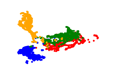
(b) Pre-adaptation

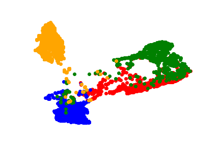
(c) Post-adaptation

Figure 2: Indirect distribution matching in the embedding space: (a) GMM samples approximating the MMWHS MR latent distribution, (b) CT latent embedding prior to adaptation (c) CT latent embedding post domain alignment. Colors correspond to: AA, LAC, LVC, MYO.

(a) GMM samples

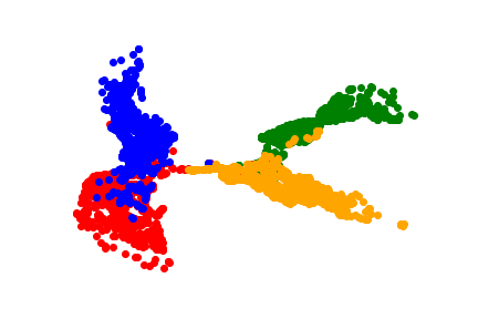
(b) Pre-adaptation

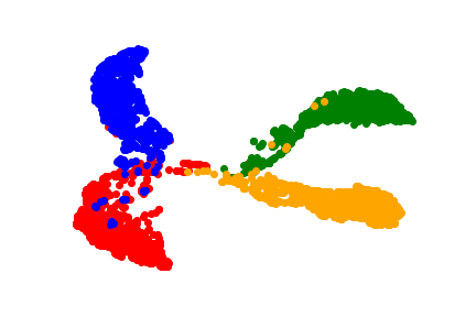
(c) Post-adaptation

Figure 3: Indirect distribution matching: (a) GMM samples approximating the CHAOS MR latent distribution, (b) Multi-Atlas CT embedding prior to adaptation (c) Multi-Atlas CT embedding post adaptation. Colors correspond to: liver, right kidney, left kidney, spleen.

(a) $\rho=0$

(b) $\rho=0.8$

(c) $\rho=.97$

Figure 4: Learnt Gaussian embeddings on the cardiac dataset for different $\rho$.

We also investigate the impact of the $\rho$ parameter on our internal distribution. In Figure 4 we present the UMAP visualization for the learnt GMM embeddings for three different values of $\rho$. We observe that while some classes will be separated for $\rho=0$, using high confidence samples to learn the GMM will yield higher separability in the internal distribution. We observe our algorithm is robust when $\rho$ is close to $1$, hence our choice of $\rho=.97$.

Ignore MYO LAC LVC AA Ignore 97.3 99.3 99.3 1.5 20.3 70.0 0.2 80.2 14.8 0.9 6.2 76.1 0.2 43.8 51.7 MYO 13.2 10.4 89.5 81.6 72.2 72.2 0.1 52.7 0.4 5.2 44.6 54.1 0.0 0.0 0.0 LAC 15.1 45.4 46.3 2.5 2.6 79.7 76.1 88.4 88.4 5.9 7.4 87.4 0.4 5.8 77.0 LVC 0.6 67.7 2.3 16.5 33.4 66.3 0.2 83.8 13.0 82.7 92.4 92.4 0.0 93.3 0.0 AA 18.5 7.8 90.9 0.0 0.0 43.7 1.3 5.7 6.2 0.1 0.0 12.9 80.1 91.2 91.2

Table 3: Percentage of shift in pixel labels during adaptation for the cardiac dataset. A cell $(i,j)$ in the table has three values. The first value represents the percentage of pixels labeled $i$ that are labeled $j$ after adaptation. The second value represents the percentage of switching pixels whose true label is $i$ - lower is better. The third value represents the percentage of switching pixels whose true label is $j$ - higher is better. Bolded cells denote label shift where more than $1\%$ of pixels migrate from $i$ to $j$.

Ignore Liver R. Kidney L. Kidney Spleen Ignore 94.6 98.4 98.4 3.0 18.0 81.6 0.7 23.5 74.3 0.7 34.9 62.6 1.0 19.3 80.5 Liver 6.6 38.1 60.8 92.6 91.3 91.3 0.8 10.4 55.1 0.0 0.0 0.0 0.0 39.0 10.2 R.Kidney 5.0 13.1 86.9 0.2 0.0 76.9 94.8 94.7 94.7 0.0 0.0 0.0 0.0 0.0 0.0 L.Kidney 2.2 24.2 75.0 0.1 0.0 0.0 0.0 23.7 0.0 97.5 87.8 87.8 0.2 0.0 7.2 Spleen 23.1 20.8 79.2 0.1 20.2 0.0 0.2 75.0 0.0 0.0 69.4 0.0 76.6 78.7 78.7

Table 4: Percentage of shift in pixel labels during adaptation for the abdominal organ dataset. The same methodology as in Table 3 is used.

The outcome of pixel label shift is analyzed in Tables 3 and 4. In Table 3 we observe that for the cardiac dataset there exists significant inter-class label transfer, for approximately $20\%$ of pixels, evenly distributed across classes. We see the majority of these shifts leading to an improvement in labeling accuracy, including all shifts where at least $1\%$ of labels migrate, which is in line with our other reported results. These findings also corroborate with our observed embeddings. We can see from Table 3 that during adaptation there is significant label migration between LVC and MYO, and this can be observed in the increased separation between the two classes in Figures 2(b) and 2(c). For the abdominal organ dataset we observe significantly less label shift between classes, with most of the activity involving previously labeled pixels being correctly le-labeled as Ignore after adaptation, or pixels initially in Ignore being correctly le-labeled to their appropriate class.

We also perform an ablative experiment for the $\omega$ parameter using the the cardiac dataset in Table 5. We observe a large increase in performance when using more than one component per class. However, this benefit decreases as more components are employed. We observe using more than $2$ components increases the Dice score, and more than a $30\%$ drop in ASSD. We conclude a larger number of class components can offer a more expressive approximation of the source distribution, leading to improvements for segmentation accuracy and organ border quality. In our study we choose $\omega=3$ to balance performance and complexity.

Full experimental setup and additional results are provided in the appendix.

Dice Average Symmetric Surface Distance $\omega$-SFS AA LAC LVC MYO Average AA LAC LVC MYO Average 1-SFS 86.2 83.5 75.4 70.9 79.0 11.1 5.0 10.8 3.6 9.8 3-SFS 88.0 83.7 81.0 72.5 81.3 6.3 7.2 4.7 6.1 6.1 5-SFS 88.0 83.8 81.9 73.3 81.7 6.2 7.4 4.8 5.7 6.0 7-SFS 86.8 84.8 82.0 73.5 81.8 4.8 7.2 4.4 5.6 5.9

Table 5: Segmentation performance versus $\omega$ for the Cardiac MR $\rightarrow$ CT adaptation task.

Figure 5: Segmentation maps of CT samples. The first five columns correspond to cardiac images, and last five correspond to abdominal images. From top to bottom: gray-scale CT images, source-only predictions, post-adaptation predictions, supervised predictions on the CT data, ground truth.

6 Conclusion

We developed a novel UDA algorithm for semantic segmentation of confidential medical data. Our idea is based on estimating the source internal distribution via a GMM and then using is to align source and target domains indirectly. We provided a empirical analysis to demonstrate why our method is effective and it leads to competitive performance on two real-world datasets when compared to state of the art approaches in medical semantic segmentation that require joint access to source and target data for adaptation.

7 Appendix

7.1 Experimental Setup

We use the same network architecture on both the cardiac and organ image segmentation UDA task. We use a DeepLabV3 [Chen et al.(2017)Chen, Papandreou, Kokkinos, Murphy, and Yuille] feature extractor with a VGG16 backbone [Simonyan and Zisserman(2015)], followed by a one layer classifier.

We train the network on the supervised source samples with a training schedule of $30,000$ epochs repeated $3$ times. The optimizer of choice is Adam with learning rate $1e-4$, $\epsilon=1e-6$ and decay of $1e-6$. We use the standard pixel-wise cross entropy loss, and batch size of $16$. For the abdominal organ segmentation dataset, we observed better performance by using a weighted cross entropy loss.

We learn the empirical internal distribution using a parameter $\rho=.97$. We observed good separability in the latent distribution for $\rho\geq.9$.

We use $\omega=3$ components per each of the $K$ classes, though as seen in Table 5, a larger $\omega$ could potentially lead to further performance gains. $\omega=3$ strikes a balance between the complexity of the GMM model and realized performance.

Finally, when performing adaptation, we performed $35,000$ epochs of training, with a batch size of $32$. We again use an Adam optimizer with a learning rate of $5e-5$, $\epsilon=1e-1$ and decay of $1e-6$. Due to GPU memory constraints leading to a limited amount of image slices per batch, and therefore a large label distribution shifts between target batches, when sampling from the learnt GMMs we approximate the target distribution via the batch label distribution.

Experiments were done on a NVIDIA RTX 3090 GPU. Code is provided in the supplementary material section of this submission, and will be made freely available online at a later date.

7.2 Additional Ablation Studies

We further empirically analyze different components of our approach to demonstrate their effectiveness.

Fine-tuning the classifier. As we discussed in the main body of the paper, after learning an internal distribution characterizing the source embeddings, we align the target embeddings to this distribution by minimizing Sliced Wasserstein Distance. In addition, we also further train the classifier on samples from this distribution to account for differences to the original source embedding distribution. We next discuss the benefit of fine tuning the classifier, based on the results in Table 6.

Metric Fine-Tuned Classifier Source Domain Classifier Dice 81.3 80.9 ASSD 6.1 7.35

Table 6: Target performance on the MMWHS adaptation task of our method with and without fine tuning the classifier on samples from the internal distribution. Bolded values indicate best performance.

Given the learnt empirical means and covariances for the internal distribution, we compare the performance after target domain adaptation between a model that fine tunes the classifier and a model that does not update the classifier after source training. As expected, fine tuning the classifier offers a prediction boost, even if the difference is not a significant one. The internal distribution is meant to encourage the target embeddings to share a similar latent space with the source embeddings, and fine tuning the classifier accounts for the distribution shift between the source embeddings and learnt internal distribution.

Filter visualization. We also investigate the information encoded in the convolutional filters before and after adaptation. Based on our results, we expect network filters to retain most of their structure from source training, and not alter this structure too much during distribution matching. We exemplify this in Figure 6. We record the visual characteristics of the network filters after the first two convolutional layers and the first four convolutional layers. We observe filters appear visually similar before and after adaptation, signifying image structural features learnt by the network do not undergo significant change, even though changes in filter values can be observed under the Difference columns.

Figure 6: Filter maps of a cardiac CT image before and after model adaptation. In the case of filter differences in absolute value, dark grey symbolizes lower values, while light gray symbolizes higher values.

References

- [Ayache(2017)] Nicholas Ayache. Deep learning for medical image analysis. In S. Kevin Zhou, Hayit Greenspan, and Dinggang Shen, editors, Deep Learning for Medical Image Analysis, page xxiii. Academic Press, 2017. ISBN 978-0-12-810408-8. https://doi.org/10.1016/B978-0-12-810408-8.00030-4. URL http://www.sciencedirect.com/science/article/pii/B9780128104088000304.
- [Bateson et al.(2020)Bateson, Kervadec, Dolz, Lombaert, and Ben Ayed] Mathilde Bateson, Hoel Kervadec, Jose Dolz, Hervé Lombaert, and Ismail Ben Ayed. Source-relaxed domain adaptation for image segmentation. In Medical Image Computing and Computer Assisted Intervention – MICCAI 2020, pages 490–499, Cham, 2020. Springer International Publishing.
- [Bateson et al.(2022)Bateson, Kervadec, Dolz, Lombaert, and Ayed] Mathilde Bateson, Hoel Kervadec, Jose Dolz, Hervé Lombaert, and Ismail Ben Ayed. Source-free domain adaptation for image segmentation. Medical Image Analysis, page 102617, 2022.
- [Bertinetto et al.(2016)Bertinetto, Valmadre, Henriques, Vedaldi, and Torr] Luca Bertinetto, Jack Valmadre, João F. Henriques, Andrea Vedaldi, and Philip H. S. Torr. Fully-convolutional siamese networks for object tracking. In Gang Hua and Hervé Jégou, editors, Computer Vision – ECCV 2016 Workshops, pages 850–865, Cham, 2016. Springer International Publishing. ISBN 978-3-319-48881-3.
- [Bousmalis et al.(2017)Bousmalis, Silberman, Dohan, Erhan, and Krishnan] Konstantinos Bousmalis, Nathan Silberman, David Dohan, Dumitru Erhan, and Dilip Krishnan. Unsupervised pixel-level domain adaptation with generative adversarial networks. In Proceedings of the IEEE conference on computer vision and pattern recognition, pages 3722–3731, 2017.
- [Chen et al.(2020)Chen, Dou, Chen, Qin, and Heng] C. Chen, Q. Dou, H. Chen, J. Qin, and P. A. Heng. Unsupervised bidirectional cross-modality adaptation via deeply synergistic image and feature alignment for medical image segmentation. IEEE Transactions on Medical Imaging, 39(7):2494–2505, 2020. 10.1109/TMI.2020.2972701.
- [Chen et al.(2019a)Chen, Xie, Huang, Rong, Ding, Huang, Xu, and Huang] Chaoqi Chen, Weiping Xie, Wenbing Huang, Yu Rong, Xinghao Ding, Yue Huang, Tingyang Xu, and Junzhou Huang. Progressive feature alignment for unsupervised domain adaptation. In Proceedings of the IEEE Conference on Computer Vision and Pattern Recognition, pages 627–636, 2019a.
- [Chen et al.(2018)Chen, Dou, Chen, and Heng] Cheng Chen, Qi Dou, Hao Chen, and Pheng-Ann Heng. Semantic-aware generative adversarial nets for unsupervised domain adaptation in chest x-ray segmentation. In International workshop on machine learning in medical imaging, pages 143–151. Springer, 2018.
- [Chen et al.(2019b)Chen, Dou, Chen, Qin, and Heng] Cheng Chen, Qi Dou, Hao Chen, Jing Qin, and Pheng-Ann Heng. Synergistic image and feature adaptation: Towards cross-modality domain adaptation for medical image segmentation. In Proceedings of The Thirty-Third Conference on Artificial Intelligence (AAAI), pages 865–872, 2019b.
- [Chen et al.(2017)Chen, Papandreou, Kokkinos, Murphy, and Yuille] Liang-Chieh Chen, George Papandreou, Iasonas Kokkinos, Kevin Murphy, and Alan L Yuille. Deeplab: Semantic image segmentation with deep convolutional nets, atrous convolution, and fully connected crfs. IEEE transactions on pattern analysis and machine intelligence, 40(4):834–848, 2017.
- [Chen et al.(2020)Chen, Lian, Wang, Deng, Kuang, Fung, Gateno, Yap, Xia, and Shen] Xu Chen, Chunfeng Lian, Li Wang, Hannah Deng, Tianshu Kuang, Steve Fung, Jaime Gateno, Pew-Thian Yap, James J Xia, and Dinggang Shen. Anatomy-regularized representation learning for cross-modality medical image segmentation. IEEE Transactions on Medical Imaging, 40(1):274–285, 2020.
- [Choi et al.(2019)Choi, Kim, and Kim] Jaehoon Choi, Taekyung Kim, and Changick Kim. Self-ensembling with gan-based data augmentation for domain adaptation in semantic segmentation. In Proceedings of the IEEE international conference on computer vision, pages 6830–6840, 2019.
- [Courty et al.(2016)Courty, Flamary, Tuia, and Rakotomamonjy] Nicolas Courty, Rémi Flamary, Devis Tuia, and Alain Rakotomamonjy. Optimal transport for domain adaptation. IEEE transactions on pattern analysis and machine intelligence, 39(9):1853–1865, 2016.
- [Dou et al.(2017)Dou, Yu, Chen, Jin, Yang, Qin, and Heng] Qi Dou, Lequan Yu, Hao Chen, Yueming Jin, Xin Yang, Jing Qin, and Pheng-Ann Heng. 3d deeply supervised network for automated segmentation of volumetric medical images. Medical Image Analysis, 41:40 – 54, 2017. ISSN 1361-8415. https://doi.org/10.1016/j.media.2017.05.001. URL http://www.sciencedirect.com/science/article/pii/S1361841517300725. Special Issue on the 2016 Conference on Medical Image Computing and Computer Assisted Intervention (Analog to MICCAI 2015).
- [Dou et al.(2018)Dou, Ouyang, Chen, Chen, and Heng] Qi Dou, Cheng Ouyang, Cheng Chen, Hao Chen, and Pheng-Ann Heng. Unsupervised cross-modality domain adaptation of convnets for biomedical image segmentations with adversarial loss. In Proceedings of the 27th International Joint Conference on Artificial Intelligence (IJCAI), pages 691–697, 2018.
- [Dou et al.(2019)Dou, Ouyang, Chen, Chen, Glocker, Zhuang, and Heng] Qi Dou, Cheng Ouyang, Cheng Chen, Hao Chen, Ben Glocker, Xiahai Zhuang, and Pheng-Ann Heng. Pnp-adanet: Plug-and-play adversarial domain adaptation network at unpaired cross-modality cardiac segmentation. IEEE Access, 7:99065–99076, 2019.
- [Drossos et al.(2019)Drossos, Magron, and Virtanen] K. Drossos, P. Magron, and T. Virtanen. Unsupervised adversarial domain adaptation based on the wasserstein distance for acoustic scene classification. In 2019 IEEE Workshop on Applications of Signal Processing to Audio and Acoustics (WASPAA), pages 259–263, 2019. 10.1109/WASPAA.2019.8937231.
- [Ghifary et al.(2016)Ghifary, Kleijn, Zhang, Balduzzi, and Li] Muhammad Ghifary, W Bastiaan Kleijn, Mengjie Zhang, David Balduzzi, and Wen Li. Deep reconstruction-classification networks for unsupervised domain adaptation. In European Conference on Computer Vision, pages 597–613. Springer, 2016.
- [Han et al.(2021)Han, Qi, Yu, Zhou, Zheng, Shi, and Gao] Xiaoting Han, Lei Qi, Qian Yu, Ziqi Zhou, Yefeng Zheng, Yinghuan Shi, and Yang Gao. Deep symmetric adaptation network for cross-modality medical image segmentation. IEEE transactions on medical imaging, 41(1):121–132, 2021.
- [Hecker et al.(2018)Hecker, Dai, and Van Gool] Simon Hecker, Dengxin Dai, and Luc Van Gool. End-to-end learning of driving models with surround-view cameras and route planners. In Proceedings of the European Conference on Computer Vision (ECCV), September 2018.
- [Hoffman et al.(2018)Hoffman, Tzeng, Park, Zhu, Isola, Saenko, Efros, and Darrell] Judy Hoffman, Eric Tzeng, Taesung Park, Jun-Yan Zhu, Phillip Isola, Kate Saenko, Alexei Efros, and Trevor Darrell. Cycada: Cycle-consistent adversarial domain adaptation. In International conference on machine learning, pages 1989–1998. PMLR, 2018.
- [Huo et al.(2018)Huo, Xu, Bao, Assad, Abramson, and Landman] Yuankai Huo, Zhoubing Xu, Shunxing Bao, Albert Assad, Richard G Abramson, and Bennett A Landman. Adversarial synthesis learning enables segmentation without target modality ground truth. In 2018 IEEE 15th international symposium on biomedical imaging (ISBI 2018), pages 1217–1220. IEEE, 2018.
- [Huo et al.(2019)Huo, Xu, Moon, Bao, Assad, Moyo, Savona, Abramson, and Landman] Yuankai Huo, Zhoubing Xu, Hyeonsoo Moon, Shunxing Bao, Albert Assad, Tamara K. Moyo, Michael R. Savona, Richard G. Abramson, and Bennett A. Landman. Synseg-net: Synthetic segmentation without target modality ground truth. IEEE Transactions on Medical Imaging, 38(4):1016–1025, Apr 2019. ISSN 1558-254X. 10.1109/tmi.2018.2876633. URL http://dx.doi.org/10.1109/TMI.2018.2876633.
- [Kamnitsas et al.(2017a)Kamnitsas, Baumgartner, Ledig, Newcombe, Simpson, Kane, Menon, Nori, Criminisi, Rueckert, and Glocker] Konstantinos Kamnitsas, Christian Baumgartner, Christian Ledig, Virginia Newcombe, Joanna Simpson, Andrew Kane, David Menon, Aditya Nori, Antonio Criminisi, Daniel Rueckert, and Ben Glocker. Unsupervised domain adaptation in brain lesion segmentation with adversarial networks. In Marc Niethammer, Martin Styner, Stephen Aylward, Hongtu Zhu, Ipek Oguz, Pew-Thian Yap, and Dinggang Shen, editors, Information Processing in Medical Imaging, pages 597–609, Cham, 2017a. Springer International Publishing.
- [Kamnitsas et al.(2017b)Kamnitsas, Baumgartner, Ledig, Newcombe, Simpson, Kane, Menon, Nori, Criminisi, Rueckert, et al.] Konstantinos Kamnitsas, Christian Baumgartner, Christian Ledig, Virginia Newcombe, Joanna Simpson, Andrew Kane, David Menon, Aditya Nori, Antonio Criminisi, Daniel Rueckert, et al. Unsupervised domain adaptation in brain lesion segmentation with adversarial networks. In International conference on information processing in medical imaging, pages 597–609. Springer, 2017b.
- [Kavur et al.(2019)Kavur, Selver, Dicle, Barıs, and Gezer] Ali Emre Kavur, M Alper Selver, Oguz Dicle, Mustafa Barıs, and N Sinem Gezer. Chaos-combined (ct-mr) healthy abdominal organ segmentation challenge data, Apr 2019. URL https://doi.org/10.5281/zenodo.3362844.
- [Kazeminia et al.(2020)Kazeminia, Baur, Kuijper, van Ginneken, Navab, Albarqouni, and Mukhopadhyay] Salome Kazeminia, Christoph Baur, Arjan Kuijper, Bram van Ginneken, Nassir Navab, Shadi Albarqouni, and Anirban Mukhopadhyay. Gans for medical image analysis. Artificial Intelligence in Medicine, 109:101938, 2020. ISSN 0933-3657. https://doi.org/10.1016/j.artmed.2020.101938. URL http://www.sciencedirect.com/science/article/pii/S0933365719311510.
- [Ker et al.(2018)Ker, Wang, Rao, and Lim] J. Ker, L. Wang, J. Rao, and T. Lim. Deep learning applications in medical image analysis. IEEE Access, 6:9375–9389, 2018. 10.1109/ACCESS.2017.2788044.
- [Kim and Canny(2017)] Jinkyu Kim and John Canny. Interpretable learning for self-driving cars by visualizing causal attention. In Proceedings of the IEEE International Conference on Computer Vision (ICCV), Oct 2017.
- [Kundu et al.(2020)Kundu, Venkat, Babu, et al.] Jogendra Nath Kundu, Naveen Venkat, R Venkatesh Babu, et al. Universal source-free domain adaptation. In Proceedings of the IEEE/CVF Conference on Computer Vision and Pattern Recognition, pages 4544–4553, 2020.
- [Kundu et al.(2021)Kundu, Kulkarni, Singh, Jampani, and Babu] Jogendra Nath Kundu, Akshay Kulkarni, Amit Singh, Varun Jampani, and R. Venkatesh Babu. Generalize then adapt: Source-free domain adaptive semantic segmentation. In Proceedings of the IEEE/CVF International Conference on Computer Vision (ICCV), pages 7046–7056, October 2021.
- [Landman et al.(2015)Landman, Xu, Igelsias, Styner, Langerak, and Klein] Bennett Landman, Z Xu, JE Igelsias, M Styner, TR Langerak, and A Klein. Multi-atlas labeling beyond the cranial vault-workshop and challenge, 2015.
- [Le et al.(2019)Le, Habrard, and Sebban] Tien-Nam Le, Amaury Habrard, and Marc Sebban. Deep multi-wasserstein unsupervised domain adaptation. Pattern Recognition Letters, 125:249 – 255, 2019. ISSN 0167-8655. https://doi.org/10.1016/j.patrec.2019.04.025. URL http://www.sciencedirect.com/science/article/pii/S0167865519301400.
- [LeCun et al.(2015)LeCun, Bengio, and Hinton] Yann LeCun, Yoshua Bengio, and Geoffrey Hinton. Deep learning. nature, 521(7553):436–444, 2015.
- [Lee et al.(2019)Lee, Batra, Baig, and Ulbricht] Chen-Yu Lee, Tanmay Batra, Mohammad Haris Baig, and Daniel Ulbricht. Sliced wasserstein discrepancy for unsupervised domain adaptation. In Proceedings of the IEEE Conference on Computer Vision and Pattern Recognition, pages 10285–10295, 2019.
- [Lin et al.(2017)Lin, Milan, Shen, and Reid] Guosheng Lin, Anton Milan, Chunhua Shen, and Ian Reid. Refinenet: Multi-path refinement networks for high-resolution semantic segmentation. In Proceedings of the IEEE conference on computer vision and pattern recognition, pages 1925–1934, 2017.
- [Liu et al.(2020)Liu, Zhang, Song, Zhang, O’Donnell, Huang, Chen, and Cai] D. Liu, D. Zhang, Y. Song, F. Zhang, L. O’Donnell, H. Huang, M. Chen, and W. Cai. Pdam: A panoptic-level feature alignment framework for unsupervised domain adaptive instance segmentation in microscopy images. IEEE Transactions on Medical Imaging, pages 1–1, 2020. 10.1109/TMI.2020.3023466.
- [Liu et al.(2011)Liu, Xiong, Pulli, and Shapiro] Dingding Liu, Yingen Xiong, Kari Pulli, and Linda Shapiro. Estimating image segmentation difficulty. In International Workshop on Machine Learning and Data Mining in Pattern Recognition, pages 484–495. Springer, 2011.
- [Long et al.(2015)Long, Shelhamer, and Darrell] Jonathan Long, Evan Shelhamer, and Trevor Darrell. Fully convolutional networks for semantic segmentation. In Proceedings of the IEEE conference on computer vision and pattern recognition, pages 3431–3440, 2015.
- [Ma et al.(2019)Ma, Zhang, and Xu] Xinhong Ma, Tianzhu Zhang, and Changsheng Xu. Gcan: Graph convolutional adversarial network for unsupervised domain adaptation. In Proceedings of the IEEE/CVF Conference on Computer Vision and Pattern Recognition (CVPR), June 2019.
- [McInnes et al.(2020)McInnes, Healy, and Melville] Leland McInnes, John Healy, and James Melville. Umap: Uniform manifold approximation and projection for dimension reduction, 2020.
- [Motiian et al.(2017)Motiian, Jones, Iranmanesh, and Doretto] Saeid Motiian, Quinn Jones, Seyed Iranmanesh, and Gianfranco Doretto. Few-shot adversarial domain adaptation. In Advances in Neural Information Processing Systems, pages 6670–6680, 2017.
- [Noh et al.(2015)Noh, Hong, and Han] Hyeonwoo Noh, Seunghoon Hong, and Bohyung Han. Learning deconvolution network for semantic segmentation. In Proceedings of the IEEE international conference on computer vision, pages 1520–1528, 2015.
- [Pan et al.(2019)Pan, Yao, Li, Wang, Ngo, and Mei] Yingwei Pan, Ting Yao, Yehao Li, Yu Wang, Chong-Wah Ngo, and Tao Mei. Transferrable prototypical networks for unsupervised domain adaptation. In Proceedings of the IEEE Conference on Computer Vision and Pattern Recognition, pages 2239–2247, 2019.
- [Qiu et al.(2021)Qiu, Zhang, Lin, Niu, Liu, Du, and Tan] Zhen Qiu, Yifan Zhang, Hongbin Lin, Shuaicheng Niu, Yanxia Liu, Qing Du, and Mingkui Tan. Source-free domain adaptation via avatar prototype generation and adaptation, 2021.
- [Rostami(2021a)] Mohammad Rostami. Lifelong domain adaptation via consolidated internal distribution. Advances in Neural Information Processing Systems, 34:11172–11183, 2021a.
- [Rostami(2021b)] Mohammad Rostami. Transfer Learning Through Embedding Spaces. CRC Press, 2021b.
- [Rostami(2022)] Mohammad Rostami. Increasing model generalizability for unsupervised domain adaptation. In Proceedings of the Conference on Lifelong Learning Agents, 2022.
- [Rostami and Galstyan(2021)] Mohammad Rostami and Aram Galstyan. Domain adaptation for sentiment analysis using increased intraclass separation. arXiv preprint arXiv:2107.01598, 2021.
- [Rostami et al.(2018)Rostami, Huber, and Lu] Mohammad Rostami, David Huber, and Tsai-Ching Lu. A crowdsourcing triage algorithm for geopolitical event forecasting. In Proceedings of the 12th ACM Conference on Recommender Systems, pages 377–381, 2018.
- [Rostami et al.(2019)Rostami, Kolouri, Eaton, and Kim] Mohammad Rostami, Soheil Kolouri, Eric Eaton, and Kyungnam Kim. Deep transfer learning for few-shot sar image classification. Remote Sensing, 11(11):1374, 2019.
- [Saito et al.(2018)Saito, Watanabe, Ushiku, and Harada] Kuniaki Saito, Kohei Watanabe, Yoshitaka Ushiku, and Tatsuya Harada. Maximum classifier discrepancy for unsupervised domain adaptation. In Proceedings of the IEEE Conference on Computer Vision and Pattern Recognition, pages 3723–3732, 2018.
- [Saltori et al.(2020)Saltori, Lathuiliére, Sebe, Ricci, and Galasso] Cristiano Saltori, Stéphane Lathuiliére, Nicu Sebe, Elisa Ricci, and Fabio Galasso. Sf-uda 3d: Source-free unsupervised domain adaptation for lidar-based 3d object detection. In 2020 International Conference on 3D Vision (3DV), pages 771–780. IEEE, 2020.
- [Sankaranarayanan et al.(2018)Sankaranarayanan, Balaji, Castillo, and Chellappa] Swami Sankaranarayanan, Yogesh Balaji, Carlos D Castillo, and Rama Chellappa. Generate to adapt: Aligning domains using generative adversarial networks. In Proceedings of the IEEE Conference on Computer Vision and Pattern Recognition, pages 8503–8512, 2018.
- [Shen et al.(2017)Shen, Wu, and Suk] Dinggang Shen, Guorong Wu, and Heung-Il Suk. Deep learning in medical image analysis. Annual Review of Biomedical Engineering, 19(1):221–248, 2017. 10.1146/annurev-bioeng-071516-044442. URL https://doi.org/10.1146/annurev-bioeng-071516-044442. PMID: 28301734.
- [Simonyan and Zisserman(2015)] Karen Simonyan and Andrew Zisserman. Very deep convolutional networks for large-scale image recognition, 2015.
- [Stan and Rostami(2021)] Serban Stan and Mohammad Rostami. Unsupervised model adaptation for continual semantic segmentation. In Proceedings of the AAAI Conference on Artificial Intelligence, volume 35, pages 2593–2601, 2021.
- [Sun et al.(2017a)Sun, Feng, and Saenko] Baochen Sun, Jiashi Feng, and Kate Saenko. Correlation alignment for unsupervised domain adaptation. In Domain Adaptation in Computer Vision Applications, pages 153–171. Springer, 2017a.
- [Sun et al.(2017b)Sun, Guo, Zhang, Li, Chen, Ma, Jin, Liu, Li, and Qian] Changjian Sun, Shuxu Guo, Huimao Zhang, Jing Li, Meimei Chen, Shuzhi Ma, Lanyi Jin, Xiaoming Liu, Xueyan Li, and Xiaohua Qian. Automatic segmentation of liver tumors from multiphase contrast-enhanced ct images based on fcns. Artificial Intelligence in Medicine, 83:58 – 66, 2017b. ISSN 0933-3657. https://doi.org/10.1016/j.artmed.2017.03.008. URL http://www.sciencedirect.com/science/article/pii/S0933365716305930. Machine Learning and Graph Analytics in Computational Biomedicine.
- [Toldo et al.(2020)Toldo, Maracani, Michieli, and Zanuttigh] Marco Toldo, Andrea Maracani, Umberto Michieli, and Pietro Zanuttigh. Unsupervised domain adaptation in semantic segmentation: A review. Technologies, 8(2):35, Jun 2020. ISSN 2227-7080. 10.3390/technologies8020035.
- [Tomar et al.(2021)Tomar, Lortkipanidze, Vray, Bozorgtabar, and Thiran] Devavrat Tomar, Manana Lortkipanidze, Guillaume Vray, Behzad Bozorgtabar, and Jean-Philippe Thiran. Self-attentive spatial adaptive normalization for cross-modality domain adaptation. IEEE Transactions on Medical Imaging, 2021.
- [Tsai et al.(2018)Tsai, Hung, Schulter, Sohn, Yang, and Chandraker] Y.-H. Tsai, W.-C. Hung, S. Schulter, K. Sohn, M.-H. Yang, and M. Chandraker. Learning to adapt structured output space for semantic segmentation. In IEEE Conference on Computer Vision and Pattern Recognition (CVPR), 2018.
- [Tzeng et al.(2017)Tzeng, Hoffman, Saenko, and Darrell] Eric Tzeng, Judy Hoffman, Kate Saenko, and Trevor Darrell. Adversarial discriminative domain adaptation. In Proceedings of the IEEE conference on computer vision and pattern recognition, pages 7167–7176, 2017.
- [Venkateswara et al.(2017)Venkateswara, Eusebio, Chakraborty, and Panchanathan] Hemanth Venkateswara, Jose Eusebio, Shayok Chakraborty, and Sethuraman Panchanathan. Deep hashing network for unsupervised domain adaptation. In Proceedings of the IEEE Conference on Computer Vision and Pattern Recognition, pages 5018–5027, 2017.
- [Wu et al.(2018)Wu, Han, Lin, Uzunbas, Goldstein, Lim, and Davis] Zuxuan Wu, Xintong Han, Yen-Liang Lin, Mustafa Gökhan Uzunbas, Tom Goldstein, Ser Nam Lim, and Larry S. Davis. Dcan: Dual channel-wise alignment networks for unsupervised scene adaptation. In Vittorio Ferrari, Martial Hebert, Cristian Sminchisescu, and Yair Weiss, editors, Computer Vision – ECCV 2018, pages 535–552, Cham, 2018. Springer International Publishing.
- [Yang et al.(2021)Yang, Wang, van de Weijer, Herranz, and Jui] Shiqi Yang, Yaxing Wang, Joost van de Weijer, Luis Herranz, and Shangling Jui. Generalized source-free domain adaptation, 2021.
- [Yilmaz et al.(2006)Yilmaz, Javed, and Shah] Alper Yilmaz, Omar Javed, and Mubarak Shah. Object tracking: A survey. ACM Comput. Surv., 38(4):13–es, December 2006. ISSN 0360-0300. 10.1145/1177352.1177355. URL https://doi.org/10.1145/1177352.1177355.
- [Zhang et al.(2019)Zhang, Chen, Huang, Lin, and Zhang] Junyi Zhang, Ziliang Chen, Junying Huang, Liang Lin, and Dongyu Zhang. Few-shot structured domain adaptation for virtual-to-real scene parsing. In Proceedings of the IEEE International Conference on Computer Vision Workshops, pages 0–0, 2019.
- [Zhang et al.(2018a)Zhang, Ouyang, Li, and Xu] Weichen Zhang, Wanli Ouyang, Wen Li, and Dong Xu. Collaborative and adversarial network for unsupervised domain adaptation. In Proceedings of the IEEE Conference on Computer Vision and Pattern Recognition (CVPR), June 2018a.
- [Zhang et al.(2018b)Zhang, Ouyang, Li, and Xu] Weichen Zhang, Wanli Ouyang, Wen Li, and Dong Xu. Collaborative and adversarial network for unsupervised domain adaptation. In Proceedings of the IEEE Conference on Computer Vision and Pattern Recognition, pages 3801–3809, 2018b.
- [Zhang et al.(2017)Zhang, David, and Gong] Yang Zhang, Philip David, and Boqing Gong. Curriculum domain adaptation for semantic segmentation of urban scenes. 2017 IEEE International Conference on Computer Vision (ICCV), Oct 2017. 10.1109/iccv.2017.223. URL http://dx.doi.org/10.1109/ICCV.2017.223.
- [Zhang et al.(2018c)Zhang, Miao, Mansi, and Liao] Yue Zhang, Shun Miao, Tommaso Mansi, and Rui Liao. Task driven generative modeling for unsupervised domain adaptation: Application to x-ray image segmentation. In International Conference on Medical Image Computing and Computer-Assisted Intervention, pages 599–607. Springer, 2018c.
- [Zhao et al.(2019)Zhao, Li, Wan, Sekuboyina, Hu, Tetteh, Piraud, and Menze] Yu Zhao, Hongwei Li, Shaohua Wan, Anjany Sekuboyina, Xiaobin Hu, Giles Tetteh, Marie Piraud, and Bjoern Menze. Knowledge-aided convolutional neural network for small organ segmentation. IEEE journal of biomedical and health informatics, 23(4):1363–1373, 2019.
- [Zhou et al.(2019)Zhou, Li, Bai, Wang, Chen, Han, Fishman, and Yuille] Yuyin Zhou, Zhe Li, Song Bai, Chong Wang, Xinlei Chen, Mei Han, Elliot Fishman, and Alan Yuille. Prior-aware neural network for partially-supervised multi-organ segmentation, 2019.
- [Zhu et al.(2018)Zhu, Yang, Liu, Kim, Zhang, and Yang] Ji Zhu, Hua Yang, Nian Liu, Minyoung Kim, Wenjun Zhang, and Ming-Hsuan Yang. Online multi-object tracking with dual matching attention networks. In Proceedings of the European Conference on Computer Vision (ECCV), September 2018.
- [Zhu et al.(2020)Zhu, Park, Isola, and Efros] Jun-Yan Zhu, Taesung Park, Phillip Isola, and Alexei A. Efros. Unpaired image-to-image translation using cycle-consistent adversarial networks, 2020.
- [Zhuang and Shen(2016)] Xiahai Zhuang and Juan Shen. Multi-scale patch and multi-modality atlases for whole heart segmentation of mri. Medical Image Analysis, 31:77 – 87, 2016. ISSN 1361-8415. https://doi.org/10.1016/j.media.2016.02.006. URL http://www.sciencedirect.com/science/article/pii/S1361841516000219.
- [Zou et al.(2020)Zou, Zhu, and Yan] Danbing Zou, Qikui Zhu, and Pingkun Yan. Unsupervised domain adaptation with dual scheme fusion network for medical image segmentation. In Proceedings of the Twenty-Ninth International Joint Conference on Artificial Intelligence, IJCAI-20, International Joint Conferences on Artificial Intelligence Organization, pages 3291–3298, 2020.