Abstract

We show that in a two-dimensional model of quantum gravity the summation over all possible wormhole configurations leads to a kind of Coleman mechanism where the cosmological constant plays no role for large universes. Observers who are unable to observe the change in topology will naturally interpret the measurements of the size of the universe as being caused by a fluctuating cosmological constant, rather than fluctuating topology of spacetime.

PACS: 04.60.Ds, 04.60.Kz, 04.06.Nc, 04.62.+v.
Keywords: quantum gravity, low dimensional models, lattice models.

1 Introduction

In a quantum theory of gravity it has always been a problem how to think of the change of topology of spacetime. Should such changes be allowed in the quantum theory of gravity? Presently, we do not know if a theory of four-dimensional quantum gravity exists an sich, or whether it has to be a part of a large theory, like string theory. It is even difficult to discuss precisely what the change of topology is supposed to mean, since if we talk about differential manifolds one cannot even in principle classify such topologies. Of course one could restrict by hand the class of manifolds and geometries such that a discussion makes some sense, or one could argue that manifolds and geometries are only derived, approximate long distance concepts coming from a different underlying theory, maybe again from string theory. However, even in string theory we are facing this problem. String theory can be viewed as two-dimensional quantum gravity coupled to certain matter fields, and in this case we know, expanding around a fixed spacetime background, that we, by the requirement of unitarity, have to sum over all two-dimensional topologies of the string. Thus viewed as a two-dimensional theory of gravity, it is a gravity theory where we have to sum over topologies. We do not know how to do this in an unambiguous way. Such a summation is usually divergent and no physical principle has so far told us uniquely how to perform such summation. This is even true in the toy models called non-critical string theories, although in these theories one can formally in many cases perform a summation over genera and find a non-perturbative partition function. In this article we will consider an even simpler “string field theory” where it is also possible to perform the summation over all genera, and we will show that from the point of view of “one-dimensional observers” such a world, where spatial universes can split and merge, appears as a world with a fluctuating cosmological constant. Also, the model provides an explicit example where one can test the so-called Coleman mechanism, which loosely states that summing over all wormholes of a theory of quantum gravity the effective cosmological constant must be zero. As we will see this is true, but maybe not the way Coleman had in mind. The rest of the article is organized as follows: in Sec. 2 we describe the so-called CDT string field theory and the result of summing over all topologies. In Sec. 3 we show that some of the results of the CDT string field theory can be obtained in a simple way by allowing the cosmological “constant” to fluctuate. Finally Sec. 4 contains a discussion of the results.

2 CDT string field theory

Causal dynamical triangulations (CDT) is an attempt to provide a non-perturbative lattice regularization of quantum gravity. In the model one can rotate to spacetimes of Euclidean signature and the four-dimensional model can be studied by computer Monte Carlo methods. Some interesting results have been obtained (see [1, 2] for reviews). Here we will be interested in the two-dimensional toy model. It can be solved analytically, and the continuum limit, where the lattice spacing goes to zero can be taken [3, 4]. The continuum theory, which can be shown to correspond to a particular sector [5] of two-dimensional Horava-Lifshitz gravity [6], is simple, and it describes the propagation of a closed one-dimensional spatial universe of length $\ell(t)$ as a function of the proper time $t$ used. The Hamiltonian is given by

$${\hat{H}}_{0}(\ell)=-\ell\frac{\mbox{d}^{2}}{\mbox{d}\ell^{2}}+\lambda\;\ell.$$ (1)

This is a standard Hermitian operator on wave functions $\psi(\ell)$ on the positive real axis, which are square-integrable with respect to the scalar product

$$\langle\psi_{1}|\psi_{2}\rangle=\int_{0}^{\infty}\frac{\mbox{d}\ell}{\ell}\;\psi^{*}_{1}(\ell)\psi_{2}(\ell).$$ (2)

The amplitude of a universe which starts out at time $t=0$ having spatial volume (length) $\ell$, i.e. in a quantum state $|\ell\rangle$, will evolve (in Euclidean time) according to

$$G_{0}(\ell,\ell^{\prime};t)=\langle\ell^{\prime}|\mbox{e}^{-t{\hat{H}}_{0}(\ell)}|\ell\rangle.$$ (3)

A complete set of eigenfunctions for ${\hat{H}}_{0}$ with corresponding eigenvalues are of the form

$$\psi_{n}^{(0)}(\ell)=p_{n}(\ell)\;\mbox{e}^{-\sqrt{\lambda}\;\ell},\quad E_{0}(n)=2n\sqrt{\lambda},\quad n=1,2,\ldots,$$ (4)

where $p_{n}(\ell)$ is a polynomial of order $n$ and $p_{n}(0)=0$. In particular, $p_{1}(\ell)=2\sqrt{\lambda}\,\ell$. The so-called Hartle-Hawking wave function is defined as

$$w_{0}(\ell)=\int_{0}^{\infty}\!\!\mbox{d}t\;G_{0}(\ell,\ell^{\prime}=0;t)=\mbox{e}^{-\sqrt{\lambda}\;\ell},\qquad{\hat{H}}_{0}(\ell)w_{0}(\ell)=0.$$ (5)

Formally the Hartle-Hawking wave function $w_{0}(\ell)$ is an eigenfunction of ${\hat{H}}_{0}$ with eigenvalue $E_{0}(0)=0$. However, it is not normalizable according to the definition (2). The Hartle-Hawking wave function $w_{0}(\ell)$ describes a universe which starts out in the state $|\ell\rangle$ and eventually disappears. The evolution of a universe, governed by (3) is such that if the universe starts out as a circle of length $\ell$, the topology of space will not change. The spatial universe cannot split in two and it cannot merge with another universe.

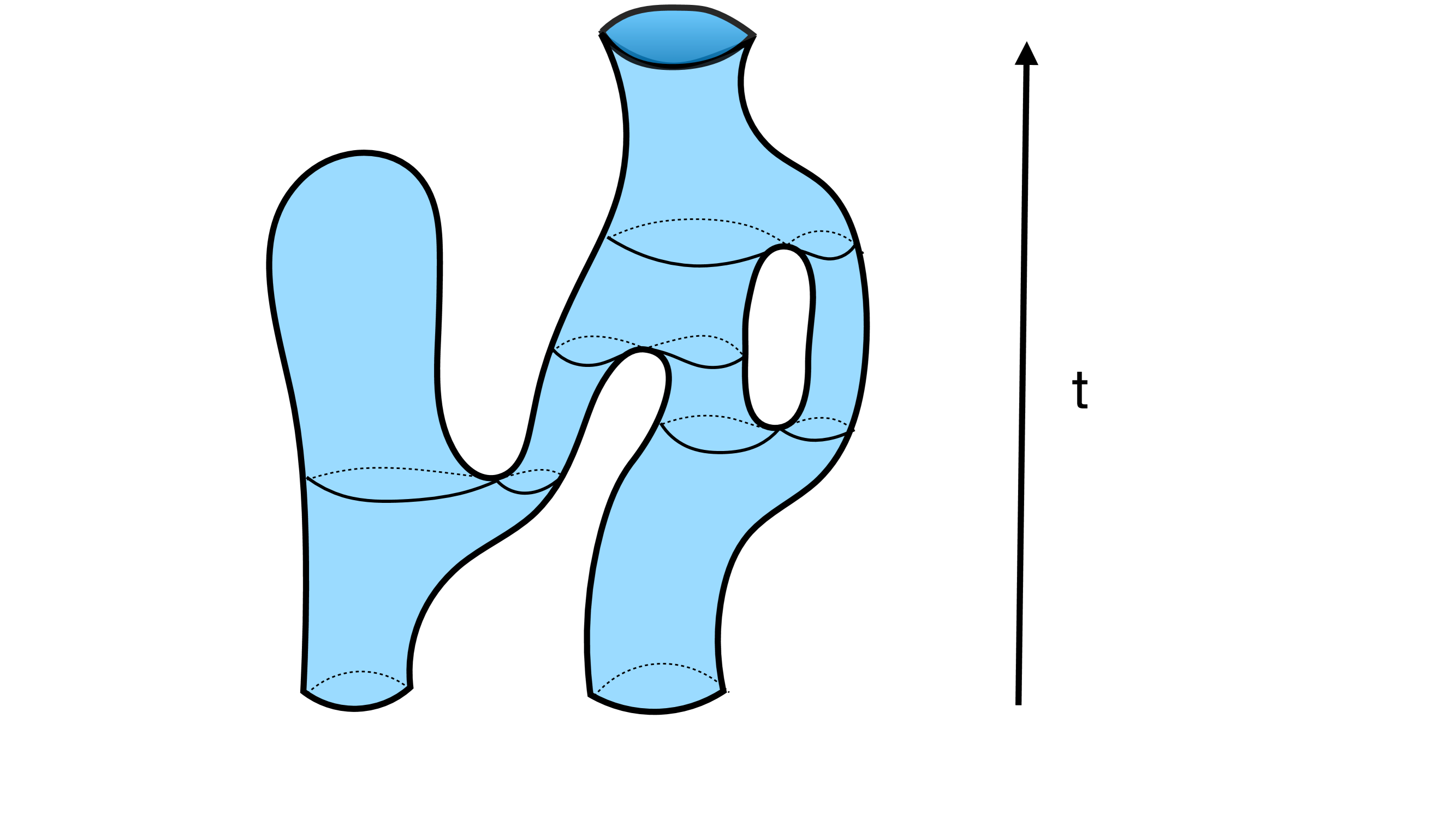
Figure 1: Dynamics of two spatial universes according to (9). At time $t=0$ we have two spatial universes, universe 1 and 2. Both propagate according to the first term in (9). At a later time the left universe (universe 1) splits into two according to the third term in (9). The left of these again propagates according to the first term, but then disappears in the vacuum, a process made possible by the the second term (a tadpole term) in (9). Universe 2 likewise splits in two, of which the left part merges with the right split of universe 1, a process made possible by the fourth term in (9). Then one of these universes merges with the universe at the right of the picture, according to the fourth term in (9). Finally this universe merges with the right split of universe 2. During this time evolution the number of spatial universes at a given time changes from 2 at $t=0$, to 3 at the first split, to 4 at the second split and then to 3 and 2 at the following mergers and finally to one when the left universe disappears in the vacuum.

The possibility to generalize this picture, such that baby universes were created was considered [7], and it was shown to be connected to a certain matrix model (it even defined a new continuum limit of matrix models) in [8]. In [9] it was developed into a full CDT string field theory, or a third quantization in the terminology of quantum gravity, where spatial universes can split and merge, governed by a “string coupling constant” $g$. More precisely, one introduces a “multi-universe” Fock space, where $\Psi^{\dagger}(\ell)$ creates one closed spatial universe of length $\ell$ with a marked point, and $\Psi(\ell)$ annihilates one closed spatial universe with no marked points (the marking and not-marking of these spatial loops are just for combinatorial convenience when solving the models). The commutation relations of the universe (or string) operators are

$$\big{[}\,\Psi(\ell)\,,\Psi^{\dagger}(\ell^{\prime})\,\big{]}\,=\,\delta(\ell-\ell^{\prime})\,,$$ (6)

$$\big{[}\,\Psi(\ell)\,,\Psi(\ell^{\prime})\,\big{]}\,=\,\big{[}\,\Psi^{\dagger}(\ell)\,,\Psi^{\dagger}(\ell^{\prime})\,\big{]}\,=\,0\,.$$ (7)

The vacuum states (no string states), in analogy with the no particle states in many body theory, are denoted $|{\rm vac}\rangle$ and $\langle{\rm vac}|$ and are the Fock states defined by

$$\Psi(\ell)|{\rm vac}\rangle\,=\,\langle{\rm vac}|\Psi^{\dagger}(\ell)\,=\,0\,.$$ (8)

The string field Hamiltonian acting on this Fock space is

$${\cal H}\! = \!\int\limits_{0}^{\infty}\!\frac{d\ell}{\ell}{\hskip 1.11206pt}\Psi^{\dagger}(\ell){\hskip 0.55603pt}{\hat{H}}_{0}(\ell)\,\ell\Psi(\ell)-\int\limits_{0}^{\infty}\!d\ell{\hskip 1.11206pt}\delta(\ell){\hskip 0.55603pt}\Psi(\ell)$$ (9)

$$\!-\;g\!\int\limits_{0}^{\infty}\!d\ell_{1}\!\int\limits_{0}^{\infty}\!d\ell_{2}{\hskip 1.11206pt}\Psi^{\dagger}(\ell_{1}){\hskip 0.55603pt}\Psi^{\dagger}(\ell_{2}){\hskip 0.55603pt}(\ell_{1}{}+{}\ell_{2})\Psi(\ell_{1}{}+{}\ell_{2})$$

$$\!-\;{\hskip 0.55603pt}g\!\int\limits_{0}^{\infty}\!d\ell_{1}\!\int\limits_{0}^{\infty}\!d\ell_{2}{\hskip 1.11206pt}\Psi^{\dagger}(\ell_{1}{}+{}\ell_{2}){\hskip 0.55603pt}\ell_{1}\Psi(\ell_{1}){\hskip 0.55603pt}\ell_{2}\Psi(\ell_{2})\,.$$

In this theory one can in principle calculate any amplitude for a universe to merge, split or disappear in the vacuum. The power of $g$ will indicate the total number of splitting and merging and one can develop a perturbation theory, where $G_{0}(\ell,\ell^{\prime};t)$ acts as the free propagator. We have illustrated a process in Fig. 1. In particular it is possible to consider the amplitude where $n$ spatial universes of length $\ell_{1},\ell_{2},\ldots,\ell_{n}$ present at $t=0$ evolve in all possible ways and eventually disappears. The connected part of this amplitude is a generalization of $w_{0}(\ell)$, which we denote $w(\ell_{1},\ldots,\ell_{n})$. In [9] it was shown that this amplitude is precisely the so-called $n$-loop amplitude of the matrix model defined in [8] and in [10] it was shown that $w(\ell_{1},\ldots,\ell_{n})$ can be found non-perturbatively and can be expressed entirely in terms of the one-loop amplitude $w(\ell)$. Further, in [11] it was shown that the results to all orders in the string coupling constant $g$ could be described as by a change of the Hamiltonian ${\hat{H}}_{0}$ to a new “non-perturbative” Hamiltonian

$${\hat{H}}_{0}(\ell)=-\ell\frac{\mbox{d}^{2}}{\mbox{d}\ell^{2}}+\lambda\;\ell\quad\to\quad{\hat{H}}(\ell)=-\ell\frac{\mbox{d}^{2}}{\mbox{d}\ell^{2}}+\lambda\;\ell-g\ell^{2}.$$ (10)

In particular, we have for the Hartle-Hawking wave function

$${\hat{H}}_{0}(\ell)w_{0}(\ell)=0\quad\to\quad{\hat{H}}(\ell)w(\ell)=0,$$ (11)

where ( Ai and Bi denote the standard Airy functions)

$$\quad w_{0}(\ell)=\mbox{e}^{-\sqrt{\lambda}\;\ell}\quad\to\quad w(\ell)=\frac{{\rm Bi}\left(\frac{\lambda-g\,\ell}{g^{2/3}}\right)}{{\rm Bi}\left(\frac{\lambda}{g^{2/3}}\right)}+c\cdot{\rm Ai}\left(\frac{\lambda-g\,\ell}{g^{2/3}}\right).$$ (12)

It is seen that $w(\ell)$ has an asymptotic expansion in $\xi=g/\lambda^{3/2}$, starting with $w_{0}(\ell)$. This is illustreted in Fig. 2.

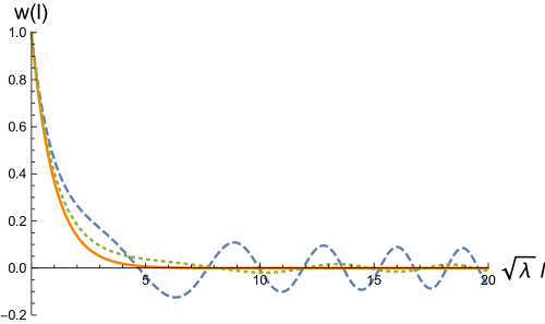
Figure 2: $y$-axis: $w_{0}(\ell)$ (orange, continuous line) and $w(\ell)$ with $c=0$ for $\xi=1/6$ (green dotted line) and $\xi=1/3$ (blue dashed line). $x$-axis: $\sqrt{\lambda}\,\ell$.

The first terms agree with the ones calculated perturbatively using CDT string field theory. $c$ is an arbitrary constant which is not determined by the perturbative expansion in $g$ (which is all we know from first principle).

The Hamiltonian ${\hat{H}}$ is unbounded from below and it has a one-parameter of self-adjoint extensions which still have a discrete spectrum $E(n)$ with corresponding eigenfunctions $\psi_{n}(\ell)$ (see [12] for a discussion of this in a similar situation in Liouville gravity and the “ordinary” double scaling limit of matrix models). A WKB analysis shows that as long as $E_{n}<\sqrt{\lambda}/(4\xi)$, $E(n)\approx E_{0}(n)$ and in addition $\psi_{n}(\ell)$ is well approximated by $\psi^{(0)}_{n}(\ell)$ provided $\sqrt{\lambda}\,\ell<1/\xi$. For $\sqrt{\lambda}\,\ell>1/\xi$ the exponential fall off of $\psi_{n}^{(0)}(\ell)$ is replaced by an oscillatory behavior where $\psi_{n}(\ell)$ only falls off like $1/\ell^{1/4}$ (in agreement with the behavior of $w(\ell)$ from (12)). This implies that while the spatial extension of a typical universe at a given time $t$ for a state $\psi_{n}^{(0)}(\ell)$ was of order $1/\sqrt{\lambda}$, the spatial extension of a typical universe for the state $\psi_{n}(\ell)$ will be infinite. In addition this dramatic change is caused by infinite order $g$ contributions. To any finite perturbative order in $g$ we would still find a spatial extension of order $1/\sqrt{\lambda}$. From a CDT string field point of view this change of behavior thus comes from infinite order change of the spatial topology. If we naively assume that “we”, as one-dimensional observers, can measure $\langle\ell(t)\rangle$, we should see quite a difference depending on wether the evolution of the universe is governed by ${\hat{H}}_{0}$ or by ${\hat{H}}$.

3 A fluctuating cosmological constant

The quantum mechanics corresponding to the hamiltonian ${\hat{H}}_{0}$ is reproduced by the path integral

$$G_{0}(\ell,\ell^{\prime};t)=\int_{\{\ell(s)\}}{\cal D}\ell(s)\;\mbox{e}^{-S[\ell(s)]},\qquad{\cal D}\ell(s)=\prod_{s=0}^{s=t}\frac{\mbox{d}\ell(s)}{\ell(s)},$$ (13)

where the integral is over functions $\ell(s)$ where $\ell(0)=\ell$ and $\ell(t)=\ell^{\prime}$, and where

$$S_{0}[\ell(s)]=\int_{0}^{t}\mbox{d}s\;\Big{(}\frac{\dot{\ell}^{2}}{4\ell(s)}+\lambda\ell(s)\Big{)},\qquad\dot{\ell}=\frac{\mbox{d}\ell(s)}{\mbox{d}s},$$ (14)

(see [13] and [5] for details). Assume now that the cosmological coupling constant is not really constant, but a variable which performs Gaussian fluctuations in time $t$ around the value $\lambda$ with a standard deviation $\sigma=2\sqrt{g}$. This would change the propagator in (13) to

$$G(\ell,\ell^{\prime};t) = \int{\cal D}\nu(s){\cal D}\ell(s)\;\exp\left[-\int_{0}^{t}\mbox{d}s\Big{(}\frac{\dot{\ell}^{2}}{4\ell(s)}+(\lambda+\nu(s))\ell(s)+\frac{1}{4g}\nu^{2}(s)\Big{)}\right]$$ (15)

$$= \int{\cal D}\ell(s)\;\exp\left[-\int_{0}^{t}\mbox{d}s\Big{(}\frac{\dot{\ell}^{2}}{4\ell(s)}+\lambda\ell(s)-g\;\ell^{2}(s)\Big{)}\right],$$

where we recall that we have assume $g\geq 0$. The resulting unboundedness of the effective potential $\lambda\ell-g\ell^{2}$ can be traced to the fact that even for a small standard deviation $\sigma=2\sqrt{g}$ there is a non-zero probability that the cosmological term $\lambda+\nu(t)$ can be negative, resulting in a term which is unbounded from below when $\ell\to\infty$. It is also seen from the effective Lagrangian appearing in (15) that for the functional integral to be well defined, the boundary conditions on $\ell(t)$ at infinity has to such that the kinetic term counteracts the unboundedness of the potential. Such a behavior at $\ell\to\infty$ is precisely the one we described in Sec. 2. We can now determine the quantum Hamiltonian corresponding to the propagator (15) by standard methods as in [13], and we find

$$G(\ell,\ell^{\prime};t)=\langle\ell^{\prime}|\mbox{e}^{-t{\hat{H}}(\ell)}|\ell\rangle,\qquad{\hat{H}}(\ell)=-\ell\frac{\mbox{d}^{2}}{\mbox{d}\ell^{2}}+\lambda\;\ell-g\ell^{2},$$ (16)

i.e. precisely the Hamiltonian (10) derived from CDT string field theory. We thus have the remarkable situation that a “trivially” fluctuating gravitational constant produces a result identical to the summation over all possible merging and splitting of space in a third quantized theory of quantum gravity. This result was observed before, where it was interpreted in the contest of stochastic quantization [14, 11], but here we want to change the perspective as discussed in the next section.

4 Do wormholes matter for your universe?

According to what is known as Coleman’s mechanism [15], we owe our whole existence to wormholes and baby universes (for a review, see, e.g. [16]). The possibility that our universe can create so-called baby universes only weakly connected to our universe or create wormholes connecting different parts of the universe is responsible for the smallness of the cosmological constant according to the Coleman mechanism. This “prediction” of the consequences of quantum fluctuations of geometry has not really been tested since we so far lack a model of quantum gravity which allows for sufficient detailed calculations in four dimensions. However, the theory of two-dimensional quantum gravity has a different status. It is a renormalizable theory, it allows for the creation of baby universes and wormholes, both in the case of 2d Euclidean quantum gravity (Liouville quantum gravity) and the case of Horava-Lifshitz gravity. Both quantum theories can be derived as scaling limits of lattice regularized versions of the theories, and the fact that these regularized versions of the theories can be solved combinatorially allows us to perform the summation over all topologies and study the effect of such a summation (see [19] for a review of the combinatorial view on these models). As mentioned above CDT is the lattice regularization of two-dimensional Horava-Lifshitz gravity, and it allowed to solve some aspects of the complete third quantization of the gravity theory, defined by the string field Hamiltonian ${\cal H}$ given in eq. (9). Let us now discuss what the solution tells us about Coleman’s mechanism. We can use the Hartle-Hawking wave function $w(\ell)$ as a starting point. It is not normalizable, but this is a short distance problem and we will be interested in large $\ell$. Alternatively we could use one of the energy eigenstates for ${\hat{H}}$, which is normalizable. As mentioned the expansion parameter is $\xi=g/\lambda^{3/2}$ and as long as $\sqrt{\lambda}\,\ell\ll 1/\xi$ the relative probability distribution of $\ell$ dictated by $w(\ell)$ follows that of $w_{0}(\ell)=e^{-\sqrt{\lambda}\,\ell}$. However for $\sqrt{\lambda}\,\ell\geq 1/\xi$ it is drastically different, to the extent that $w(\ell)$ does not fall off exponentially but only as $1/\ell^{1/4}$. In fact the large $\ell$ behavior depends on the dimensionless variable $\sqrt{g}\,\ell^{3/2}$, rather than on $\sqrt{\lambda}\,\ell$. Thus we can say that the large scale structure of the universe is independent of the cosmological constant $\lambda$ and it not governed by the exponential behavior associated with $\lambda$. In this sense Coleman’s mechanism is working: the cosmological constant is irrelevant for the large scale structure. What is not quite like the simplest version of Coleman’s mechanism is that the resulting large scale structure is not simply given by a classical background where one puts the cosmological constant to zero. The infinite genus universes seem to play a crucial role, and this is true no matter how small the expansion parameter $\xi$ is. Eventually, for $\sqrt{\lambda}\,\ell\gg 1/\xi$ infinite genus surfaces dominate the behavior of $w(\ell)$ and all the eigenfunctions $\psi_{n}(\ell)$ of ${\hat{H}}$.

Let us image that we are one-dimensional beings living in a universe where $g=0$. The Hamiltonian is thus ${\hat{H}}_{0}$ and if the universe is in the lowest energy eigenstate state $\psi_{1}^{(0)}(\ell)$ then a number of measurements of the spatial volume (length) $\ell(t)$ of our universe at times $t_{1},t_{2},\ldots$ will result in a distribution $P^{(0)}_{1}(\ell)=\big{(}\psi_{1}^{(0)}(\ell)\big{)}^{2}/\ell=4\lambda\,\ell\,\mbox{e}^{-2\sqrt{\lambda}\ell}$. If one had a model for the universe, stating that the quantum evolution is governed by ${\hat{H}}_{0}$ and that the universe is in the energy state corresponding to the eigenvalue $E_{0}(1)$ of ${\hat{H}}_{0}$, then the observations would allow us to determine the cosmological constant $\lambda$. If, in reality, $g>0$, but $\xi\ll 1$ and the universe was in the energy state $\psi_{1}(\ell)$ of ${\hat{H}}$, then as long as we can only measure $\ell$s where $\sqrt{\lambda}\,\ell\ll 1/\xi$ we would reach the same conclusion. However, as our measurements improved and we could measure larger and larger values of $\ell$, we would observe disagreement with the predictions coming from ${\hat{H}}_{0}$. Assuming that we were never able to actually observe a change in topology, we would be tempted to conclude that our observations support the idea that the cosmological constant is actually not constant, but fluctuating like $\lambda(t)=\lambda+\nu(t)$. That assumption would result in an effective, but weird Hamiltonian ${\hat{H}}$, unbounded from below and it would explain the observed distribution $P_{1}(\ell)=\big{(}\psi_{1}(\ell)\big{)}^{2}/\ell$ of measured $\ell$. Still one would most likely say that a picture provided by the string field Hamiltonian ${\cal H}$, given by (9) is much more satisfactory, and it allows potentially for a detailed description of the dynamics of merging and splitting of universes. It also calls for a better understanding of what kind of infinite genus spacetime will actually appear and be important in our model. This question can actually be addressed because the model is so simple, and preliminary results [20] indicate that these spacetimes are in some sense “nice” infinite genus spacetimes [21]. We believe that research in this direction could be important both for “real” string theory and for models where two-dimensional CDT is used to construct higher dimensional universes [22, 23]. As an example, let us mention that it follows from the models considered in [22, 23] that if the wavelength of a typical oscillation of the cosmological constant is larger than a couple of billion years, our theory suggests that the present acceleration of our universe can be explained by the summation over baby universes and wormholes in CDT, in this way unifying physics at the shortest distances and at the largest scales. Details of such an estimate will appear in a separate publication.

References

- [1] J. Ambjorn, A. Goerlich, J. Jurkiewicz and R. Loll, Phys. Rept. 519 (2012), 127-210, [arXiv:1203.3591 [hep-th]].
- [2] R. Loll, Class. Quant. Grav. 37 (2020) no.1, 013002, [arXiv:1905.08669 [hep-th]].
- [3] J. Ambjorn, R. Loll, Nucl. Phys. B 536 (1998) 407-434, [hep-th/9805108].
- [4] J. Ambjorn and T. G. Budd, J. Phys. A: Math. Theor. 46 (2013), 315201, [arXiv:1302.1763 [hep-th]].
- [5] J. Ambjorn, L. Glaser, Y. Sato and Y. Watabiki, Phys. Lett. B 722 (2013), 172-175, [arXiv:1302.6359 [hep-th]].
-
[6]
P. Hořava,
Phys. Rev. D 79 (2009) 084008,
[arXiv:0901.3775, hep-th].
P. Hořava and C.M. Melby-Thompson, Phys. Rev. D 82 (2010) 064027, [arXiv:1007.2410, hep-th]. - [7] J. Ambjorn, R. Loll, W. Westra and S. Zohren, JHEP 0712 (2007) 017 [arXiv:0709.2784, gr-qc].
-
[8]
J. Ambjorn, R. Loll, W. Westra and S. Zohren,
Phys. Lett. B 665 (2008) 252-256 [arXiv:0804.0252, hep-th];
Phys. Lett. B 670 (2008) 224 [arXiv:0810.2408, hep-th]. - [9] J. Ambjorn, R. Loll, Y. Watabiki, W. Westra and S. Zohren: JHEP 0805 (2008) 032 [arXiv:0802.0719, hep-th].
- [10] J. Ambjorn, R. Loll, W. Westra and S. Zohren, Phys. Lett. B 678 (2009), 227-232, [arXiv:0905.2108 [hep-th]].
- [11] J. Ambjorn, R. Loll, W. Westra and S. Zohren, Phys. Lett. B 680 (2009), 359-364, [arXiv:0908.4224 [hep-th]].
- [12] J. Ambjorn and C. F. Kristjansen, Int. J. Mod. Phys. A 8 (1993), 1259-1282, [arXiv:hep-th/9205073 [hep-th]].
- [13] J. Ambjorn and A. Ipsen, Phys. Lett. B 724 (2013), 150-154, [arXiv:1302.2440 [hep-th]].
- [14] M. Ikehara, N. Ishibashi, H. Kawai, T. Mogami, R. Nakayama and N. Sasakura, Phys. Rev. D 50 (1994), 7467-7478, [arXiv:hep-th/9406207 [hep-th]]; Prog. Theor. Phys. Suppl. 118 (1995), 241-258, [arXiv:hep-th/9409101 [hep-th]].
- [15] S. R. Coleman, Nucl. Phys. B 310 (1988) 643.
- [16] A. Hebecker, T. Mikhail and P. Soler, Front. Astron. Space Sci. 5 (2018), 35 doi:10.3389/fspas.2018.00035 [arXiv:1807.00824 [hep-th]].
- [17] H. Kawai and T. Okada, Int. J. Mod. Phys. A 26 (2011), 3107-3120 doi:10.1142/S0217751X11053730 [arXiv:1104.1764 [hep-th]].
- [18] H. Kawai and T. Okada, Prog. Theor. Phys. 127 (2012), 689-721 doi:10.1143/PTP.127.689 [arXiv:1110.2303 [hep-th]].
- [19] J. Ambjorn, B. Durhuus and T. Jonsson, Quantum geometry. A statistical field theory approach. Cambridge University Press, Cambridge, 1997.
- [20] J. Ambjorn, Y. Sato and Y. Watabiki, to appear.
- [21] J. Feldman, H. Knörrer and E. Trubowitz, Riemann Surfaces of Infinite Genus, CRM Monograph series, American Mathematical Society, 2003.
- [22] J. Ambjørn and Y. Watabiki, Nucl. Phys. B 955 (2020), 115044, [arXiv:2003.13527 [hep-th]];
- [23] J. Ambjorn and Y. Watabiki, Mod. Phys. Lett. A 32 (2017) no.40, 1750224, [arXiv:1709.06497 [gr-qc]]; Phys. Lett. B 770 (2017), 252-256, [arXiv:1703.04402 [hep-th]]; Phys. Lett. B 749 (2015), 149-152, [arXiv:1505.04353 [hep-th]].