A Nearby Galaxy Perspective on Dust Evolution

Abstract

Context. The efficiency of the different processes responsible for the evolution of interstellar dust on the scale of a galaxy, are to date very uncertain, spanning several orders of magnitude in the literature. Yet, a precise knowledge of the grain properties is the key to addressing numerous open questions about the physics of the interstellar medium and galaxy evolution.

Aims. This article presents an empirical statistical study, aimed at quantifying the timescales of the main cosmic dust evolution processes, as a function of the global properties of a galaxy.

Methods. We have modelled a sample of $\simeq 800$ nearby galaxies, spanning a wide range of metallicity, gas fraction, specific star formation rate and Hubble stage. We have derived the dust properties of each object from its spectral energy distribution. Through an additional level of analysis, we have inferred the timescales of dust condensation in core-collapse supernova ejecta, grain growth in cold clouds and dust destruction by shock waves. Throughout this paper, we have adopted a hierarchical Bayesian approach, resulting in a single large probability distribution of all the parameters of all the galaxies, to ensure the most rigorous interpretation of our data.

Results. We confirm the drastic evolution with metallicity of the dust-to-metal mass ratio (by two orders of magnitude), found by previous studies. We show that dust production by core-collapse supernovae is efficient only at very low-metallicity, a single supernova producing on average less than $\simeq 0.03\;\textnormal{M}_{\odot}$/SN of dust. Our data indicate that grain growth is the dominant formation mechanism at metallicity above $\simeq 1/5$ solar, with a grain growth timescale shorter than $\simeq 50$ Myr at solar metallicity. Shock destruction is relatively efficient, a single supernova clearing dust on average in at least $\simeq 1200\;\textnormal{M}_{\odot}$/SN of gas. These results are robust when assuming different stellar initial mass functions. In addition, we show that early-type galaxies are outliers in several scaling relations. This feature could result from grain thermal sputtering in hot X-ray emitting gas, an hypothesis supported by a negative correlation between the dust-to-stellar mass ratio and the X-ray photon rate per grain. Finally, we confirm the well-known evolution of the aromatic-feature-emitting grain mass fraction as a function of metallicity and interstellar radiation field intensity. Our data indicate the relation with metallicity is significantly stronger.

Conclusions. Our results provide valuable constraints for simulations of galaxies. They imply that grain growth is the likely dust production mechanism in dusty high-redshift objects. We also emphasize the determinant role of local low-metallicity systems to address these questions.

1 INTRODUCTION

Characterizing the dust properties across different galactic environments is an important milestone towards understanding the physics of the InterStellar Medium (ISM) and galaxy evolution (Galliano et al., 2018, for a review). Interstellar grains have a nefarious role of obscuring our direct view of star formation (e.g.  Bianchi et al., 2018). The subsequent unreddening of Ultraviolet-(UV)-visible observations relies on assumptions about the constitution and size distribution of the grains, as well as on the relative star-dust geometry (e.g.  Witt et al., 1992; Witt & Gordon, 2000; Baes & Dejonghe, 2001). Dust is also involved in several important physical processes, such as the photoelectric heating of the gas in PhotoDissociation Regions (PDR; e.g. Draine, 1978; Kimura, 2016) or H${}_{\textnormal{2}}$ formation (e.g.  Gould & Salpeter, 1963; Bron et al., 2014). The uncertainties about the grain properties have dramatic consequences on the rate of these processes and are the main cause of discrepancy between PDR models (Röllig et al., 2007). Finally, state-of-the-art numerical simulations of galaxy evolution are now post-processed to incorporate the full treatment of dust radiative transfer in order to reproduce realistic observables (e.g.  Camps et al., 2016, 2018; Trayford et al., 2017; Rodriguez-Gomez et al., 2019; Trčka et al., 2020). These simulations rely on assumptions about the dust emissivity, absorption and scattering properties, which changes from galaxy to galaxy (e.g.  Clark et al., 2019; Bianchi et al., 2019).

We are far from being able to predict the dust composition, structure and size distribution, in a given ISM condition. Ab initio methods are currently impractical because of the great complexity of the problem. Empirical approaches face challenges, too. The last four decades have shown that each time we were investigating a particular observable with the hope of constraining the grain properties, these properties were proving themselves more elusive because of their evolution, as illustrated in the following.

• The diversity of extinction curve shapes within the Milky Way (Fitzpatrick, 1986; Cardelli et al., 1989) and the Magellanic Clouds (Gordon et al., 2003) can be explained by variations of the size distribution and carbon-to-silicate grain ratio (Pei, 1992; Kim et al., 1994; Clayton et al., 2003; Cartledge et al., 2005).

• Elemental depletion patterns strongly depend on the density of the medium, suggesting that dust is partly destroyed and reformed in the ISM (Savage & Mathis, 1979; Crinklaw et al., 1994; Jenkins, 2009; Parvathi et al., 2012).

• Variations of the InfraRed (IR) to submillimeter (submm) emissivity as a function of the density of the medium, whether in the Milky Way (Stepnik et al., 2003; Ysard et al., 2015) or in the Magellanic clouds (Roman-Duval et al., 2017), are interpreted as variations of the grain mantle thickness and composition, and grain-grain coagulation (e.g.  Köhler et al., 2015; Ysard et al., 2016).

• The wide variability of the relative intensity and band-to-band ratio of the mid-IR aromatic feature spectrum, witnessed within the Milky Way and nearby galaxies, is the evidence of the variation of the abundance, charge and size distribution of the band carriers (e.g.  Boulanger et al., 1998; Madden et al., 2006; Galliano et al., 2008b; Schirmer et al., 2020).

• The wavelength-dependent polarization fraction in extinction and emission provides additional constraints on the composition of the grains, as well as on their shape and alignment (e.g.  Andersson et al., 2015; Fanciullo et al., 2017).

To understand the evolution of the global dust content of a galaxy, one must be able to quantify the timescales of the processes responsible for dust formation and destruction. These processes can be categorized as follows.

Stardust production

takes place primarily in the ejecta of: 1 Asymptotic Giant Branch(AGB) stars; and 2 type II SuperNovae(SN II; core-collapse SN). SNe II potentially dominate the net stardust injection rate (e.g.  Draine, 2009, for a review), but their actual yield is the subject of an intense debate. Most of the controversy lies in the fact that, while large amounts could form in SN II ejecta (e.g.  Matsuura et al., 2015; Temim et al., 2017), a large fraction of freshly formed grains could not survive the reverse shock (e.g.  Nozawa et al., 2006; Micelotta et al., 2016; Kirchschlager et al., 2019). Estimates of the net dust yield of a single SN ranges in the literature from $\simeq 10^{-3}$ to $1\;\textnormal{M}_{\odot}/\textnormal{SN}$ (e.g.  Todini & Ferrara, 2001; Ercolano et al., 2007; Bianchi & Schneider, 2007; Bocchio et al., 2016; Marassi et al., 2019).

Grain growth

in the ISM refers to the addition of gas atoms onto pre-existing dust seeds (e.g.  Hirashita, 2012). It could be the main grain formation process, happening on timescales $\lesssim 1$ Myr (e.g.  Draine, 2009). It is however challenged due to the lack of direct constraints and because we currently lack a proven dust formation mechanism, at cold temperatures.

Grain destruction

can be attributed to: 1 astration, i.e. their incorporation into stellar interiors during star formation; 2 sputtering and shattering by SN blast waves. The second process is the most debated, although it is less controversial than stardust production and grain growth efficiencies. Timescales for grain destruction in the Milky Way range from $\simeq 200$ Myr to $\simeq 2$ Gyr (Jones et al., 1994; Slavin et al., 2015).

In the Milky Way, there is a convergent set of evidence pointing toward a scenario where: 1 stardust accounts for at most $\simeq 10\,\%$ of ISM dust; 2 most grains are therefore grown in the ISM (e.g.  Draine & Salpeter, 1979; Dwek & Scalo, 1980; Jones et al., 1994; Tielens, 1998; Draine, 2009). The goal of this paper is to explore how particular environments could affect these conclusions, by modelling nearby extragalactic systems. By studying nearby galaxies, we also aim to provide a different perspective on these questions.

Several attempts have been made in the past to quantify the evolution of the dust content of galaxies via fitting their Spectral Energy Distribution (SED; e.g. Lisenfeld & Ferrara, 1998; Morgan & Edmunds, 2003; Draine et al., 2007; Galliano et al., 2008a; Rémy-Ruyer et al., 2014, 2015; De Vis et al., 2017b; Nersesian et al., 2019; De Looze et al., 2020; Nanni et al., 2020). Although these studies provided important benchmarks, most of them were limited by the following issues: 1 their coverage of the parameter space was often incomplete, especially in the low-metallicity regime, which is crucial to quantify stardust production (cf. Sect. 5); 2 potential systematic effects, originating either in the SED fitting or in the ancillary data, were questioning some of the conclusions; 3 dust evolution models were most of the time not fit to each galaxy, but simply visually compared, which can lead to some inconsistencies (cf. Sect. 5.2.3).

The present paper is an attempt at addressing these limitations. We rely on the homogeneous multi-wavelength observations and ancillary data of the DustPedia project (Davies et al., 2017) and of the Dwarf Galaxy Sample (DGS; Madden et al., 2013). We adopt a Hierarchical Bayesian (HB; cf. Sect. 3.1) approach when comparing models to observations, in order to limit the impact of systematic effects on our results (Galliano, 2018, hereafter G18). Finally, we perform a rigorous dust evolution modelling of individual objects in our sample, in order to unambiguously constrain the dust evolution timescales. Sect. 2 presents the data we have used. Sect. 3 presents our model and discusses the robustness of the derived dust parameters. Sect. 4 provides a qualitative discussion of the derived dust evolution trends. Sect. 5 describes the quantitative modelling of the main dust evolution processes. Sect. 6 summarizes our results. Several technical arguments are detailed in the appendices, so that they do not alter the flow of the discussion.

2 THE GALAXY SAMPLE

This study focuses on global properties of galaxies. Integrating the whole emission of a galaxy complicates the interpretation of the trends, as we will discuss in Sect. 4. However, it also presents some advantages: 1 we can include galaxies unresolved at infrared wavelengths; and 2 we can provide benchmarks for comparisons to unresolved studies of the distant Universe or to one-zone dust evolution models. Several upcoming studies on a subsample of resolved DustPedia galaxies will discuss the improvements that the spatial distribution of the dust properties provides (Roychowdhury et al., in prep.; Casasola et al., in prep.).

2.1 The Infrared Photometry

We present here the integrated, multi-wavelength photometry of our sample, used to constrain the global dust properties of each galaxy. We focus on the mid-IR-to-submm regime, as it is where dust emits.

2.1.1 The DustPedia Aperture Photometry

We use the photometry of the 875 galaxies of the DustPedia sample presented by Clark et al. (2018, hereafter C18). Since we focus on the mid-IR-to-submm regime, we restrain the wavelength range to photometric bands centered between 3 $\mu\textnormal{m}$ and 1 mm. The list of photometric bands we have used is given in Table 1. C18 has provided a dedicated reduction of the Herschel broadband data and an homogenization of the Spitzer, WISE and Planck observations. Foreground stars have been masked. Aperture-matched photometry has been performed on each image and a local background has been subtracted from each flux. A consistent noise uncertainty was estimated for each measurement. IRAS fluxes from Wheelock et al. (1994) were added to the catalog. We refer the reader to C18 for more details about the data reduction and photometric measurement.

Table 1: Number of galaxies observed through each photometric band. During the inference process (Sect. 3.2), the observed fluxes are compared to the SED model integrated within the transmission of these filters, with the appropriate flux convention.

Instrument	Wavelength	Label	Number of galaxies
	(central)		3$\sigma$ detection	Total
WISE	$3.4\;\mu\textnormal{m}$	WISE1	725	751
	$4.6\;\mu\textnormal{m}$	WISE2	663	739
	$11.6\;\mu\textnormal{m}$	WISE3	554	728
	$22.1\;\mu\textnormal{m}$	WISE4	438	694
IRAC	$3.5\;\mu\textnormal{m}$	IRAC1	277	292
(Spitzer)	$4.5\;\mu\textnormal{m}$	IRAC2	359	390
	$5.7\;\mu\textnormal{m}$	IRAC3	100	113
	$7.8\;\mu\textnormal{m}$	IRAC4	116	130
MIPS	$23.7\;\mu\textnormal{m}$	MIPS1	125	178
(Spitzer)	$71\;\mu\textnormal{m}$	MIPS2	32	41
	$156\;\mu\textnormal{m}$	MIPS3	18	25
PACS	$70\;\mu\textnormal{m}$	PACS1	108	144
(Herschel)	$100\;\mu\textnormal{m}$	PACS2	273	456
	$160\;\mu\textnormal{m}$	PACS3	296	493
SPIRE	$250\;\mu\textnormal{m}$	SPIRE1	481	674
(Herschel)	$350\;\mu\textnormal{m}$	SPIRE2	446	658
	$500\;\mu\textnormal{m}$	SPIRE3	404	634
IRAS	$60\;\mu\textnormal{m}$	IRAS3	282	360
	$100\;\mu\textnormal{m}$	IRAS4	391	501
HFI	$350\;\mu\textnormal{m}$	HFI1	217	275
(Planck)	$550\;\mu\textnormal{m}$	HFI2	127	182
	$850\;\mu\textnormal{m}$	HFI3	93	125

The SED model (Sect. 3.1), that we have applied to our data, performs a complex statistical treatment, allowing us to analyze even poorly sampled SEDs. However, the efficiency of such a model can be affected by the presence of systematic effects not properly accounted for by the uncertainties. In order to be conservative, we have therefore excluded a series of fluxes, based on the following criteria.

1. The C18 catalog flags about $22\,\%$ of its fluxes, for different reasons: artefacts, contamination by nearby sources, incomplete extended emission, etc. We have excluded all the fluxes that are flagged. For 89 galaxies, all IR fluxes end up flagged. These galaxies have therefore been excluded.

2. Several galaxies contain a significant emission from their Active Galactic Nucleus (AGN). This emission is characterized by a prominent synchrotron continuum and copious amounts of hot dust ($T_{\mbox{{\scriptsize dust}}}\gtrsim 300$ K), resulting in a rather flat mid-IR continuum. Our dust model (Sect. 3.1.1) is optimized for regular interstellar dust. Our distribution of starlight intensities (Sect. 3.1.2) is usually not flexible enough to account for the hot emission from the torus. We have therefore excluded 19 sources presenting such an emission at a significant level, following Bianchi et al. (2018), who used the criterion of Assef et al. (2018) based on the WISE1 and WISE2 fluxes to identify AGNs.

3. We have performed a preliminary least-squares fit with our reference SED model (Sect. 3.3), in order to identify where the largest residuals are.

   1. A few short wavelength bands present a large deviation from their SED model and their adjacent fluxes. After inspection of the images, the discrepancies are likely due to residual starlight contamination.

   2. Several long-wavelength IRAS fluxes are significantly deviant from their nearby MIPS and PACS fluxes. The reason of these discrepancies is obscure. However, Sect. 3.3 will present a test comparing SED results with and without IRAS data, showing they are not crucial to our study.

   3. Three additional galaxies are not properly fitted. These objects present the characteristics of an AGN and are indeed classified as such (Liu & Zhang, 2002). They were not accounted for by the Assef et al. (2018) criterion. It is however consistent with the fact that this criterion has a $90\,\%$ confidence level.

   We have excluded all these problematic fluxes. Criterion 3 is more qualitative than 1 and 2, but it allows us to identify potential systematics that were missed.

In total, we are left with 764 DustPedia galaxies.

The monochromatic fluxes (in Jy) were converted to monochromatic luminosities (in $\textnormal{L}_{\odot}$/Hz), using the distances from the HyperLeda database (Makarov et al., 2014).

2.1.2 The Dwarf Galaxy Sample

Metallicity is a crucial parameter to study dust evolution (cf. Sect. 5 and Rémy-Ruyer et al., 2014, 2015). In particular, the low-metallicity regime, represented by dwarf galaxies, provides unique constraints (e.g.  Galliano et al., 2018), yet the DustPedia sample selected sources larger than 1′. In order to improve the sampling of the low-metallicity regime, we have thus included additional galaxies from the Dwarf Galaxy Survey (DGS; Madden et al., 2013).

Among the 48 sources of the DGS, 35 are not in the DustPedia sample. We have added these sources to our sample. These galaxies have been observed with Spitzer, WISE and Herschel. We use the aperture photometry presented by Rémy-Ruyer et al. (2013, 2015). We do not expect systematic differences between the DustPedia and DGS aperture fluxes. Appendix B.1 compares the photometry of the DGS sources that are in DustPedia. Both are indeed in very good agreement. Similarly to the DustPedia sample, we apply the three exclusion criteria of Sect. 2.1.1.

1. We exclude the fluxes that have been flagged.

2. No significant AGN contribution is present in this sample.

3. Rémy-Ruyer et al. (2015) advise to not trust the PACS photometry for HS 0822+3542. Since this source is neither detected with SPIRE, we simply exclude it.

In total, we are left with 34 DGS galaxies, in addition to those already included in DustPedia.

2.1.3 Photometric Uncertainties

Our combined sample contains 798 galaxies. For each of them, we consider the following two sources of photometric uncertainty.

The noise:

it includes statistical fluctuations of the detectors and residual background subtraction. It has been thoroughly estimated by C18 and Rémy-Ruyer et al. (2015). We assume that the noise of each waveband of each galaxy follows an independent normal distribution.

Calibration uncertainties:

they are systematics, i.e. fully correlated between different galaxies, and partially correlated between wavebands. We assume they follow a joint, multivariate normal distribution, whose covariance matrix is given in Appendix A.

Table 1 gives the number of galaxies observed though each waveband, and the number of detections (flux greater than $3\sigma$, where $\sigma$ refers solely to the noise uncertainty). The number of available filters per galaxy ranges between 1 and 19, and its median is 11. There is a median number of 2 upper limits per galaxy.

2.2 The Ancillary Data

We present here the ancillary data gathered in order to characterize the ISM conditions in each galaxy.

2.2.1 The Stellar Mass

For the DustPedia sample, we adopt the stellar masses of Nersesian et al. (2019). Theses masses were derived from UV-to-mm SED fitting, using the code CIGALE (Boquien et al., 2019), with two stellar populations. For the DGS, the stellar masses are given by Madden et al. (2014), using the Eskew et al. (2012) relation, based on the IRAC1 and IRAC2 fluxes. Eskew et al. (2012) emphasize that the largest source of systematic uncertainties in the stellar mass is the Initial Mass Function (IMF). Both Nersesian et al. (2019) and Eskew et al. (2012) adopt a Salpeter (1955) IMF, therefore limiting potential biases between the two samples. Other potential biases, such as the form of the assumed star formation history, should not be an issue with our sample. For instance, both Mitchell et al. (2013) and Laigle et al. (2019) tested the reliability of stellar mass estimates using numerical simulations of galaxies, and showed that they gave consistent results at low redshift. We use $M_{\star}$ to denote the stellar mass.

Nanni et al. (2020, hereafter N20) have reestimated the stellar masses of the DGS, with CIGALE. They report systematically lower values, compared to Madden et al. (2014), sometimes by an order of magnitude. We discuss the possible reasons of this discrepancy in Appendix B.2, concluding that our estimates are likely more reliable.

2.2.2 The Metallicity

For DustPedia galaxies, we use the metallicities derived by De Vis et al. (2019), using the $S$ calibration of Pilyugin & Grebel (2016, hereafter PG16_S). For the DGS, we use the metallicities derived by De Vis et al. (2017b), using the same PG16_S calibration. De Vis et al. (2017b) show that this particular calibration is the most reliable at low-metallicity.

We adopt the solar elemental abundances of Asplund et al. (2009): the hydrogen mass fraction is $X_{\odot}=0.7381$, the helium mass fraction, $Y_{\odot}=0.2485$, the heavy element mass fraction, $Z_{\odot}=0.0134$, and the oxygen-to-hydrogen number ratio, $12+\log(\textnormal{O/H})_{\odot}=8.69\pm 0.05$. Throughout this study, we assume a fixed elemental abundance pattern. It implies that the total metallicity, $Z$, scales with the oxygen-to-hydrogen number ratio as:

$$Z\simeq 2.04\times 10^{-9}\times 10^{12+\log(\textnormal{O/H})}\;\textnormal{Z}_{\odot}.$$ (1)

For that reason, in the rest of the paper, we refer to both $Z$ and $12+\log(\textnormal{O/H})$, as metallicity.

2.2.3 The Gas Mass

Neutral gas.

The neutral hydrogen masses, derived from [H i]${}_{21\,\textnormal{cm}}$, have been compiled by De Vis et al. (2019), for DustPedia, and Madden et al. (2013), for the DGS. Integrating the H i mass in the aperture used for the photometry is not always possible for the smallest sources, as they are not resolved by single dish observations. This is particularly important for dwarf galaxies, where the H i disk tends to be significantly larger than the optical/IR radius (e.g.  Begum et al., 2008), as we will discuss in Sect. 4.1.3. Roychowdhury et al. (in prep.) recently obtained interferometric, spatially-resolved [H i]${}_{21\,\textnormal{cm}}$ observations of 20 of the lowest-metallicity galaxies in our sample ($12+\log(\textnormal{O/H})\leq 8.0$). They integrated these H i masses in the aperture used for the photometry in order to provide a better estimate of the gas mass associated with the dust emission. We have adopted these more accurate values, for these 20 objects. We have multiplied the H i mass of each galaxy by $1/(1-Y_{\odot}-Z)\simeq 1.35$ to account for helium (assumed independent of metallicity) and heavier elements. We use $M_{\mbox{{\scriptsize H$\,${i}}}}$ to denote the total atomic gas mass probed by [H i]${}_{21\,\textnormal{cm}}$.

Molecular gas.

Casasola et al. (2020a) compiled observations of ¹²CO lines for 245 late-type DustPedia galaxies. They converted these observations in molecular masses, assuming a constant $X_{\mbox{{\scriptsize CO}}}$ conversion factor (Bolatto et al., 2013), and corrected them for aperture effects. The uncertainties are the quadratic sum of the ¹²CO line noise measurement and $30\,\%$, corresponding to the uncertainty on the $X_{\mbox{{\scriptsize CO}}}$. We adopt these values when available. For the other DustPedia and DGS galaxies, we infer the H${}_{\textnormal{2}}$ mass, with the approximation used by De Vis et al. (2019, Eq. 7). It uses the scaling relation between $M_{\mbox{{\scriptsize H$\,${i}}}}/M_{\star}$ and $M_{\mbox{{\scriptsize H${}_{\textnormal{2}}$}}}/M_{\mbox{{\scriptsize H$\,${i}}}}$, derived by Casasola et al. (2020a). The scatter of this relation is propagated and accounted for in the uncertainties. These molecular gas masses are also corrected for helium and heavy elements. We use $M_{\mbox{{\scriptsize H${}_{\textnormal{2}}$}}}^{\mbox{{\scriptsize CO}}}$ to denote the total molecular gas mass derived from actual ¹²CO line observations, and $M_{\mbox{{\scriptsize H${}_{\textnormal{2}}$}}}$, to denote the method-independent total molecular mass, either derived from ¹²CO lines or from the De Vis et al. (2019) approximation.

2.2.4 The Star Formation Rate

For DustPedia, the Star Formation Rate (SFR), has been derived by Nersesian et al. (2019). The SFR was a free parameter of the SED fit they performed with CIGALE. For the DGS, we used the SFR estimated by Rémy-Ruyer et al. (2015), using a combination of the H$\alpha$${}_{656.3\textnormal{nm}}$ line and of the Total InfraRed luminosity (TIR). Although the two estimators are different, we do not expect significant biases between DustPedia and the DGS. Indeed, both account for: 1 the escaping power from young ionizing stars, with the UV SED or the H$\alpha$${}_{656.3\textnormal{nm}}$ line; and 2 the power re-radiated by dust, with the IR SED or the TIR. In addition, both assume a Salpeter (1955) IMF, which, similarly to the stellar mass (Sect. 2.2.1), is the main source of uncertainty. We use SFR to denote the numerical value of the SFR, expressed in $\textnormal{M}_{\odot}$/yr and, $\textnormal{sSFR}\equiv\textnormal{SFR}/M_{\star}$, to denote the specific SFR.

2.2.5 Uncertainties of the Ancillary Data

The SED analysis we will present in Sect. 3.1 includes the ancillary data, as a prior. For that purpose, it is preferable to consider the logarithm of quantities that can span several orders of magnitude. The independent ancillary data parameters we use as a constraint are listed in the first five lines of Table 2. The total gas mass is $M_{\mbox{{\scriptsize gas}}}=M_{\mbox{{\scriptsize H$\,${i}}}}+M_{\mbox{{\scriptsize H${}_{\textnormal{2}}$}}}$ and the ¹²CO-line-estimated molecular fraction, $f_{\mbox{{\scriptsize H${}_{\textnormal{2}}$}}}^{\mbox{{\scriptsize CO}}}=M_{\mbox{{\scriptsize H${}_{\textnormal{2}}$}}}^{\mbox{{\scriptsize CO}}}/M_{\mbox{{\scriptsize gas}}}$. We also list, in the second part of Table 2, parameters derived from these quantities, including the method-independent molecular fraction, $f_{\mbox{{\scriptsize H${}_{\textnormal{2}}$}}}=M_{\mbox{{\scriptsize H${}_{\textnormal{2}}$}}}/M_{\mbox{{\scriptsize gas}}}$. All the extensive quantities (masses and SFR) have been homogenized to the distances adopted in Sect. 2.1.

Table 2: Number of galaxies per ancillary data constraint.

Ancillary data	Parameter	Number of galaxies
Total gas mass	$\ln M_{\mbox{{\scriptsize gas}}}$	518
Molecular fraction	$\ln f_{\mbox{{\scriptsize H${}_{\textnormal{2}}$}}}^{\mbox{{\scriptsize CO}}}$	179
Stellar mass	$\ln M_{\star}$	785
Star formation rate	$\ln\textnormal{SFR}$	749
Metallicity	$12+\log(\textnormal{O/H})$	376
Molecular fraction	$\ln f_{\mbox{{\scriptsize H${}_{\textnormal{2}}$}}}$	514
Gas-to-star ratio	$\ln(M_{\mbox{{\scriptsize gas}}}/M_{\star})$	514
Gas fraction	$\ln f_{\mbox{{\scriptsize gas}}}$	514
Specific SFR	$\ln\textnormal{sSFR}$	745

We assume that the uncertainty of the 5 independent ancillary parameters (first part of Table 2) follows a split-normal distribution ( G18, Sect. 3.2.3). We propagate the uncertainties and their correlations in the derived parameters (second part of Table 2).

3 THE SED MODELLING APPROACH

We now describe our modelling approach, as well as the consistency tests we have performed to assess the robustness of our results.

3.1 Our In-House Hierarchical Bayesian SED Model

HerBIE (HiERarchical Bayesian Inference for dust Emission; G18, ) is a hierarchical Bayesian model aimed at inferring the Probability Density Functions (hereafter PDF) of dust parameters (dust mass, etc.), from their SED, rigorously accounting for the different sources of uncertainties. As any Bayesian model, HerBIE computes a posterior PDF as the product of a classical likelihood and a prior PDF. What makes this model hierarchical is that the prior depends on a set of hyperparameters. These hyperparameters are: 1 the average of each physical parameter; and 2 their covariance matrix. The hyperparameters are inferred, together with the parameters of each individual galaxy. We are therefore sampling a single, large-dimension, joint PDF. Since the shape of the prior is inferred from the data, the information of the whole sample is used, in this process, to refine our knowledge of each individual galaxy. In particular, it is relevant to keep in our sample even poorly-constrained SEDs, with upper limits or missing fluxes. Such a model is also efficient at suppressing the numerous noise-induced, false correlations between parameters, encountered when fitting SEDs with least-squares or non-hierarchical Bayesian methods (Shetty et al., 2009; Kelly et al., 2012; Galliano, 2018; Lamperti et al., 2019). It has recently been used to study the anomalous microwave emission in the Milky Way (Bell et al., 2019).

From a technical point of view, HerBIE uses a Markov Chain Monte-Carlo (hereafter MCMC), with Gibbs sampling (Geman & Geman, 1984). As mentioned in Sect. 2.2, we include the ancillary data in our prior. This process is fully demonstrated in Sect. 5.3 of G18. These ancillary data do not enter the dust model, but they provide information that helps to better constrain the hyperparameters, in a holistic way. In other words, the information provided by the gas mass or the metallicity helps to better constrain the dust SED fit. It is a Bayesian implementation of Stein’s paradox (Stein, 1956; Efron & Morris, 1977).

3.1.1 Parametrization of the Dust Model

To infer dust parameters with HerBIE, we adopt the framework provided by the grain properties of the THEMIS model (Jones et al., 2017). THEMIS is built, as much as possible, on laboratory data, and reproduces dust observables of the Galactic ISM. One of its originalities is that it accounts for the aromatic and aliphatic mid-IR features with a single population of small, partially hydrogenated, amorphous carbons, noted a-C(:H). Consequently, it does not include Polycyclic Aromatic Hydrocarbons (PAH) per se. Although largely dehydrogenated, small a-C(:H) are very similar to PAHs. The other main component of THEMIS is a population of large, a-C(:H)-coated, amorphous silicates, with Fe and FeS nano-inclusions.

THEMIS is designed to model the evolution of: 1 the size distribution, 2 the a-C(:H) hydrogenation, and 3 the mantle thickness, with the InterStellar Radiation Field (ISRF) and gas density. With the observational constraints of Sect. 2.1, we can not reliably constrain the mantle thickness, as its effect on the shape of the far-IR SED is too subtle. Nor can we constrain the a-C(:H) hydrogenation, as broadband fluxes do not provide unambiguous constraints on the 3.4 $\mu\textnormal{m}$ feature. We can however study the variations of the size distribution of small a-C(:H), from galaxy to galaxy, as it will affect the strength of the bright mid-IR aromatic features.

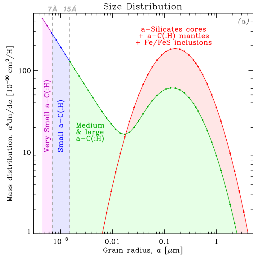
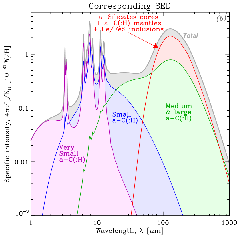
Figure 1: Parametrization of the THEMIS model. Panel (a) shows the size distribution of the two main components of THEMIS: amorphous carbons and silicates. We show how we divide the a-C(:H) size distribution into three independent components. Panel (b) shows the SED corresponding to each component (same color code as panel a). The SED is shown for the ISRF of the solar neighborhood (Mathis et al., 1983).

We have therefore parametrized the size distribution in the following way.

1. We have divided the a-C(:H) component into (cf. Fig. 1):

   Very small a-C(:H)

   (denoted VSAC) of radius smaller than 7 Å, responsible for the mid-IR feature emission, with more weight in the short wavelength bands;

   Small a-C(:H)

   (denoted SAC) of radius between 7 Å and 15 Å, responsible for the mid-IR feature emission, with more weight in the long wavelength bands;

   Medium and large a-C(:H)

   (noted MLAC) of radius larger than 15 Å, carrying the featureless mid-IR continuum and a fraction of the far-IR peak.

2. The silicate-to-MLAC ratio is kept constant.

Using $q_{X}$ to denote the mass fraction of component $X$, the size distribution is controlled by two parameters: 1 the mass fraction of aromatic-feature-carrying grains, $q_{\mbox{{\scriptsize AF}}}\equiv q_{\mbox{{\scriptsize VSAC}}}+q_{\mbox{{\scriptsize SAC}}}$; and 2 the very-small-a-C(:H)-to-aromatic-feature-emitting-grain ratio, $f_{\mbox{{\scriptsize VSAC}}}\equiv q_{\mbox{{\scriptsize VSAC}}}/q_{\mbox{{\scriptsize AF}}}$. Comparing these parameters to dust models with PAHs (e.g.  Zubko et al., 2004; Draine & Li, 2007; Compiègne et al., 2011), $q_{\mbox{{\scriptsize AF}}}$ is the analogue of the PAH mass fraction, $q_{\mbox{{\scriptsize PAH}}}$ introduced by Draine & Li (2007, hereafter DL07). The difference here is that, $q_{\mbox{{\scriptsize AF}}}=17\,\%$, while $q_{\mbox{{\scriptsize PAH}}}=4.6\,\%$, in the diffuse Galactic ISM. This is because a-C(:H) have a smaller fraction of aromatic bonds per C atom. More mass is therefore needed to produce the feature strength of a PAH.

This parametrization has the great advantage of being linear. A simpler version, fixing $f_{\mbox{{\scriptsize VSAC}}}$, has been implemented in CIGALE by Nersesian et al. (2019). A more physical way to vary the size distribution would be to vary the minimum cut-off size and the index of the power-law size distribution (cf.  Jones et al., 2013, for the description of the size distribution of THEMIS). However, this alternate parametrization would be CPU time consuming, and would not produce noticeable differences in the resulting broadband SED (cf. Appendix C).

3.1.2 The Mixing of Physical Conditions

A model, such as THEMIS, is not directly applicable to observations of galaxies. Indeed, the monochromatic flux of a whole galaxy comes from the superposition of grains exposed to a range of physical conditions. This well-known problem can be addressed assuming a distribution of starlight intensity inside each galaxy. We adopt the prescription proposed by Dale et al. (2001), where the dust mass, $M_{\mbox{{\scriptsize dust}}}$, follows a power-law distribution, as a function of the starlight intensity, $U$:

$$\textnormal{d}M_{\mbox{{\scriptsize dust}}}\propto U^{-\alpha}\,\textnormal{d}U U_{\mbox{{\scriptsize min}}}<U<U_{\mbox{{\scriptsize min}}}+\Delta U.$$ for (2)

The parameter $U$ is the frequency-integrated monochromatic mean intensity of the Mathis et al. (1983) diffuse ISRF. It is normalized so that $U=1$ in the solar neighborhood (e.g. Eq. 2 of Galliano et al., 2011). This phenomenological composite SED is the powerU model component of G18 (Sect. 2.2.5). We add to the emission the starBB component of G18 (Sect. 2.2.6), in order to account for the residual diffuse stellar emission at short wavelengths.

The list of free SED model parameters, that HerBIE infers, is thus the following. Similarly to the ancillary parameters (Table 2), we use the natural logarithm of quantities varying over more than an order of magnitude.

1. $\ln M_{\mbox{{\scriptsize dust}}}$, the dust mass, scales with the whole dust SED.

2. $\ln U_{\mbox{{\scriptsize min}}}\in[\ln 0.01,\ln 10^{3}]$ is the minimum cut-off in Eq. (2).

3. $\ln\Delta U\in[\ln 1,\ln 10^{7}]$ controls the range in Eq. (2).

4. $\alpha\in[1,2.5]$ is the power-law index in Eq. (2).

5. $\ln q_{\mbox{{\scriptsize AF}}}\in[\ln 10^{-5},\ln 0.9]$ is defined in Sect. 3.1.1.

6. $f_{\mbox{{\scriptsize VSAC}}}\in[0,1]$ is defined in Sect. 3.1.1.

7. $\ln L_{\star}$ is the luminosity of the residual stellar emission (cf.  G18, Sect. 2.2.6).

These parameters are however not the most physically relevant. In the rest of the present article, we focus our discussion on the following three parameters, marginalizing over the other ones: 1 $M_{\mbox{{\scriptsize dust}}}$; 2 $\langle U\rangle$; and 3 $q_{\mbox{{\scriptsize AF}}}$, where $\langle U\rangle$ (Eq. 9 of G18, ) is the mean of the distribution in Eq. (2). It quantifies the mass-averaged starlight intensity illuminating the grains. It is a function of the three parameters $U_{\mbox{{\scriptsize min}}}$, $\Delta U$ and $\alpha$ (Eq. 10 of G18, ). It can be related to an equivalent large grain equilibrium temperature, $T_{\mbox{{\scriptsize eq}}}$, through: $\langle U\rangle\simeq(T_{\mbox{{\scriptsize eq}}}/18\;\textnormal{K})^{5.8}$ (e.g.  Nersesian et al., 2019).

3.1.3 Questionable Assumptions and Residual Contaminations

In our experience, the model of Sect. 3.1.2 is the most appropriate for galaxies observed with the typical spectral coverage of Table 1. It presents however the following limitations.

Shape of the ISRF.

We assume that dust is heated by the Mathis et al. (1983) ISRF, scaled by a factor $U$. We assume in the model that the shape of this ISRF does not vary between galaxies nor within regions inside galaxies. It is obvious that this assumption is not correct. However, its consequences are minimal on the parameters we are interested in, for the following reasons.

• $M_{\mbox{{\scriptsize dust}}}$ and $\langle U\rangle$ depend mainly on the far-IR peak emission, which is dominated by large grains. These grains are at thermal equilibrium. Their emission therefore does not depend on the shape of the ISRF, only on the absorbed power.

• $q_{\mbox{{\scriptsize AF}}}$ controls the fraction of small, stochastically-heated grains. The emission from these grains depends on the shape of the ISRF (e.g.  Camps et al., 2015). However, since small a-C(:H) are destroyed in H ii regions (cf. Sect. 4.2.3 of Galliano et al., 2018, and Sect. 4.2), they are effectively heated by a rather narrow spectral range ($4\;\textnormal{eV}\lesssim h\nu<13.6\;\textnormal{eV}$), where they exist. This effect is demonstrated on Fig. 7 of Draine (2011), with PAHs. We thus do not expect that actual variations of the ISRF shape will significantly bias our estimate of $q_{\mbox{{\scriptsize AF}}}$.

Evolution of small a-C(:H).

The abundance of small a-C(:H) and their properties evolve with the ISRF and the gas density. These grains are dehydrogenated and destroyed by intense ISRFs; they are also accreted onto large grains, in dense regions (e.g.  Jones et al., 2013; Köhler et al., 2015). Our parametrization (Sect. 3.1.1) allows us to explore variations of $q_{\mbox{{\scriptsize AF}}}$ between galaxies, but we assume that $q_{\mbox{{\scriptsize AF}}}$ is constant, for all $U$, within each galaxy. However, this assumption will not bias our global estimate of $q_{\mbox{{\scriptsize AF}}}$, as this parameter is merely a way to give a physical meaning to the observed $L_{\mbox{{\scriptsize AF}}}/\textnormal{TIR}$ ratio ($L_{\mbox{{\scriptsize AF}}}$ denoting the power emitted by the aromatic features). This assumption would only be problematic if we were trying to estimate the local value of $q_{\mbox{{\scriptsize AF}}}$ in PDRs, for instance. Indeed, we would, in this case, underestimate $q_{\mbox{{\scriptsize AF}}}$, by assuming that a fraction of the aromatic feature emission comes from H ii regions, which are generally hotter than PDRs, and thus more emissive.

Grain opacity.

We assume that the grain opacity does not vary between galaxies, nor within regions inside galaxies. There are several indications that this hypothesis is not correct (e.g. Sect. 4.2.1 of Galliano et al., 2018). In particular, the far-IR opacity can typically vary by a factor of $\simeq 3$ with the accretion/removal of mantles and grain-grain coagulation (Köhler et al., 2015). Such variations will bias our estimate of the dust mass. In addition, the submm/mm silicate emissivity implemented in THEMIS has an unphysical power-law dependence at long wavelengths. Accounting for a more realistic opacity, based on laboratory measurements such as those of Demyk et al. (2017b, a), will likely affect our dust mass estimates. This is an important effect that we can not avoid. We discuss its consequences in Sect. 4.1.3, when interpreting our results.

Residual contaminations.

The following emission processes, not accounted for in our model, could be present in our observations.

• Several gas lines contribute to the emission in the photometric bands of Table 1. The brightest are: [O i]${}_{63\mu\textnormal{m}}$, [O iii]${}_{88\mu\textnormal{m}}$, [C ii]${}_{158\mu\textnormal{m}}$, [O i]${}_{145\mu\textnormal{m}}$ and ¹²CO(J$=$3$\rightarrow$2)${}_{867\mu\textnormal{m}}$. Without dedicated spectroscopic observations, the subtraction of these lines is hazardous. Luckily enough, their intensities are, to first order, proportional to TIR (e.g.  Cormier et al., 2015). They constitute therefore a bias proportional to the flux, that can be taken into account together with the calibration bias, as we will show in Sect. 3.2.

• The submm excess is an excess emission of debated origin, appearing longward 500 $\mu\textnormal{m}$ (cf. Sect. 3.5.5 of Galliano et al., 2018, for a review). Since it is not accounted for in our model, it could bias our submm SED. This effect is however probably negligible in our sample, for the following reasons.

  1. This submm excess is model-dependent. THEMIS has a flatter submm opacity than models based on the DL07 optical properties (e.g. Fig. 4 of Galliano et al., 2018). It is therefore more emissive in the submm regime and minimizes the contribution of the excess.

  2. This excess is observed in dwarf galaxies, but is rarely detected in higher metallicity systems (e.g.  Galliano et al., 2003, 2005; Galametz et al., 2009; Rémy-Ruyer et al., 2015; Dale et al., 2017). Yet, data longward 500 $\mu\textnormal{m}$, in our sample, are available only for large objects, due to the large Planck/HFI beam.

  3. Residuals of our model run (Sect. 3.2) do not show significant excesses in the submm bands.

• Residual stellar emission could contaminate the shortest wavelength bands. Improper stellar subtraction could lead to positive or negative offsets, independently in the different bands.

3.2 The Reference Run

Figure 2: Select SED fits. Each panel shows the inferred SED PDF, in yellow intensity scale, normalized by the MCMC-averaged TIR. The color violin plots represent the synthetic photometry PDF, for each waveband. The black error bars are the observations. Panels (a), (b) and (c) show arbitrary chosen galaxies, representative of their classes (early-type, late-type and irregulars, respectively). Panel (d) shows the case, where most constraints are only upper limits.

The results we will present in Sect. 4 are obtained with the model described in Sect. 3.1. We call it our reference run. Fig. 2 shows the SED fit of four representative objects, obtained with this run. In panels (a), (b) and (c), SEDs of three arbitrarily chosen galaxies, representative of Early-Type Galaxies (ETG), Late-Type Galaxies (LTG) and irregulars, respectively, are displayed. The PDF of the SED is shown as a yellow density plot. We also show the PDF of the synthetic photometry (violin plots of different colors). The comparison of this synthetic photometry to the observed flux (circles with an error bar) reflects the quality of the fit. We discuss a more thorough and technical fit quality test in Appendix D. Panel (d) shows the example of a galaxy where most of the fluxes are $3\sigma$-upper limits (displayed when $F_{\nu}<\sigma_{\nu}^{\mbox{{\scriptsize noise}}}$). When the evidence provided by the data is weak, which is the case when few detections are available, the posterior distribution becomes dominated by the prior. This is what we see here. The range spanned by this SED PDF is the extent of the prior. The global scaling of this SED is very uncertain, but its shape is realistic. This would not be the case with a non-hierarchical model.

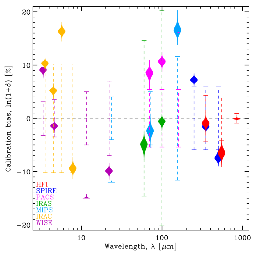
Figure 3: Inferred calibration biases. This figure shows our inference of the calibration bias, $\delta$, defined in Sect. 3.2.2 of G18, for each of the photometric filters in Table 1. Each instrument is color-coded. The vertical dashed error bars represent the calibration prior, i.e. the $\pm 1\sigma$ range given in Appendix A. The violin plots show the actual posterior PDFs of $\delta$, for each broadband. The width of a single violin plot is proportional to the PDF as a function of $\delta$ (vertical axis).

Fig. 3 shows the inference of the calibration biases, $\delta(\lambda)$, of each waveband (Sect. 2.1.3). Basically, the model fluxes are corrected by factors $1+\delta(\lambda)$. For each waveband, the dashed-line error bar represents the $\pm 1\sigma$ interval of the prior on the calibration bias. This prior is a multivariate normal distribution, centered on 0, with the covariance matrix of Eq. (18). As discussed in Sect. 3.1.3, besides accounting for the uncertainty in the calibration of each instrument, these coefficients can account for external contaminations and fitting residuals. We can interpret the most deviant values of Fig. 3 in this light. The posterior values of $\delta$ lying outside their $\pm 2\sigma$ prior are the following.

160 $\boldsymbol{\mu}$m:

both overlapping bands PACS3 and MIPS3 indicate an excess emission of about $15\,\%$. A significant fraction of this excess is likely due here to contamination by the brightest line of the ISM, [C ii]${}_{158\mu\textnormal{m}}$. The [C ii]${}_{158\mu\textnormal{m}}$ intensity is about $\simeq 1\,\%$ the FIR (far-IR; 60-200 $\mu\textnormal{m}$) power (Malhotra et al., 1997, 2001; Brauher et al., 2008; Cormier et al., 2015). Its contribution to the PACS3 and MIPS3 is thus expected to be a few percent, as these bands are narrower than the FIR range.

12 $\boldsymbol{\mu}$m and 22 $\boldsymbol{\mu}$m:

the deficit could be due to a systematic difference between the size distribution of medium a-C(:H) grains implemented in THEMIS and in the diffuse ISM of these galaxies. Although the model was different, Galliano et al. (2011, Appendix A.2) had to decrease the abundance of the grains carrying the 24 $\mu\textnormal{m}$ continuum in the Large Magellanic Cloud (LMC), for a similar reason.

Apart from these deviations, the two overlapping bands WISE1 and IRAC1 indicate that the model, on average, underestimates the observations by $\simeq 10\,\%$ around 3.5 $\mu\textnormal{m}$. This could be due to either the continuum or the 3.3/3.4 $\mu\textnormal{m}$ features. The constraint of the size distribution of THEMIS by the SED of the Milky Way (Fig. 3 of Jones et al., 2013), has been performed with a medium resolution IRS spectrum for all a-C(:H) features, except the two in question here. The global emissivity of these features is the most uncertain of the model. We also notice that the SPIRE calibration biases go in opposite directions, while they should be partially correlated (Appendix A.5). The HFI1 and HFI2 calibration biases agree very well with SPIRE. This is the sign that there is a systematic residual proportional to the flux in this wavelength range. It could mean that the slope of THEMIS is not steep enough in the $200-500\;\mu\textnormal{m}$ range. The fact that the HFI3 is almost 0 would mean that the slope flattens again longward $\simeq 800\;\mu\textnormal{m}$. This is very speculative, but we note that this behaviour is qualitatively consistent with the optical properties measured in the laboratory by Demyk et al. (2017a).

The parameters inferred with this run, for each galaxy, are given in Table H (electronic version only). We report only the parameter values and their uncertainties (mean and standard-deviation of the posterior PDF). The skewness and correlation coefficients can be retrieved from the DustPedia archive (http://dustpedia.astro.noa.gr). The length of the MCMC of this run is $1\,000\,000$, where we have excluded the first $100\,000$ steps, to account for burn-in. The maximum integrated autocorrelation time (Eq. 43 of G18, ) is $65\,000$.

3.3 Additional Runs: Robustness Assessment

In order to assess the robustness of our results, we have performed several additional runs, with different assumptions. We now discuss the comparison of these tests with our reference run. We focus on the derived dust mass and do not display the redundant comparisons with $\langle U\rangle$. Indeed, TIR is usually well constrained and, by model construction, $\textnormal{TIR}\propto M_{\mbox{{\scriptsize dust}}}\times\langle U\rangle$. We discuss the difference in $q_{\mbox{{\scriptsize AF}}}$, when relevant. Figs. 4 – 6 compares $M_{\mbox{{\scriptsize dust}}}$ or $q_{\mbox{{\scriptsize AF}}}$ derived by these tests to the same quantity derived by the reference run, $M_{\mbox{{\scriptsize dust}}}^{\mbox{{\scriptsize ref}}}$ and $q_{\mbox{{\scriptsize AF}}}^{\mbox{{\scriptsize ref}}}$, respectively. Table 3 reports some statistics on this comparison. We color code the galaxies according to their Hubble stage, $T$:

Early-type:

$T\leq 0$ (red);

Late-type:

$0<T<9$ (green);

Irregulars:

$T\geq 9$ (blue).

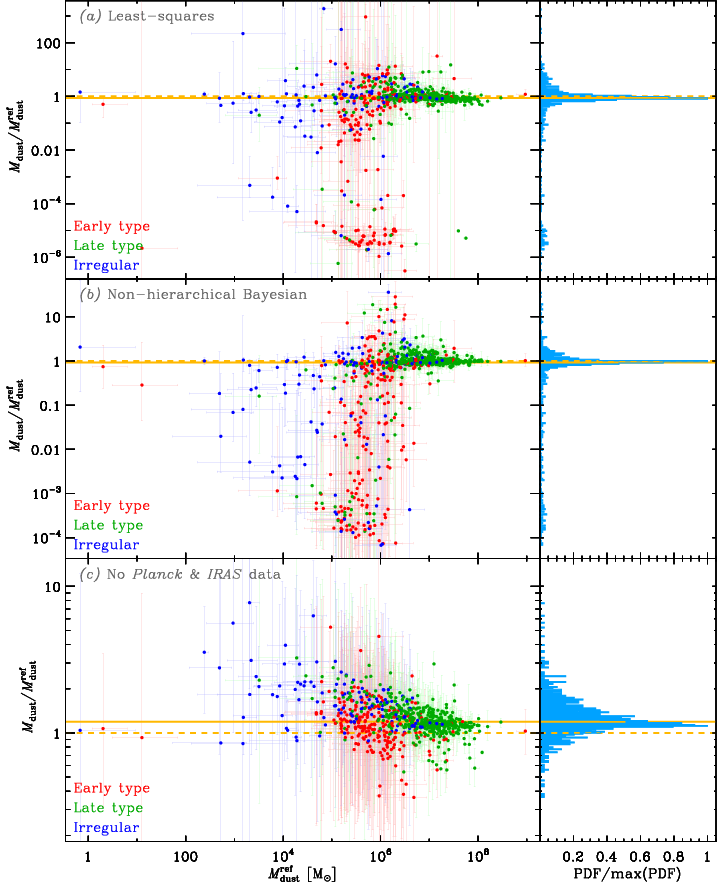
Figure 4: Robustness assessment. Each of the three horizontal panels of Figs. 4 to 6 display the comparison of the various tests of Sect. 3.3 to our reference run (Sect. 3.2). The left column panels show the ratio of either $M_{\mbox{{\scriptsize dust}}}$ or $q_{\mbox{{\scriptsize PAH}}}$, derived from the test (grey label in the top left corner), to its equivalent with the reference run, as a function of $M_{\mbox{{\scriptsize dust}}}^{\mbox{{\scriptsize ref}}}$. Galaxies are color-coded according to their type. The right column plot shows the PDF (normalized) of the distribution of the ratio. The median of the ratio is displayed as an orange solid line. The 1:1 ratio is highlighted as an orange dashed line. This figure shows the influence of various fitting methods.

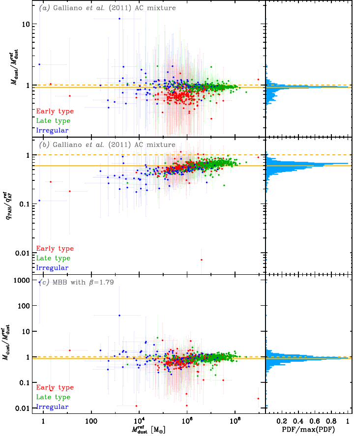
Figure 5: Same as Fig. 4. This figure shows the influence of various fitting methods.

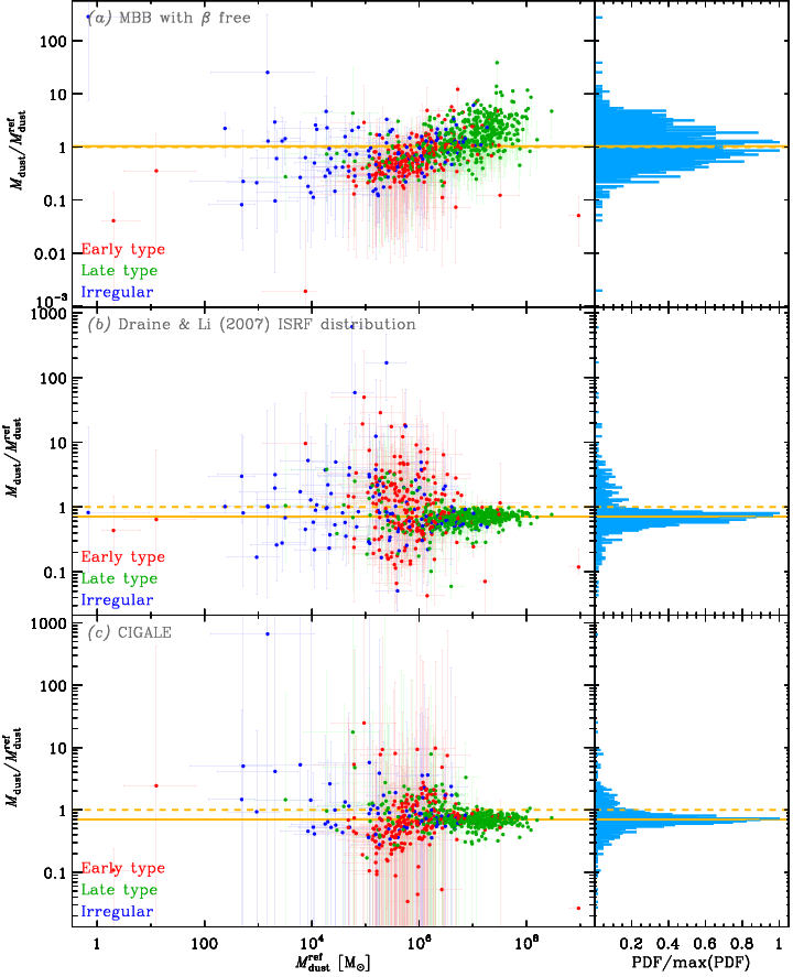
Figure 6: Same as Fig. 4. The first two panels continue to show the influence of various dust model assumptions as in Fig. 4. The other panel is a comparison with results from a previous work done using the same sample but different method.

Table 3: Robustness assessment. Statistics of the comparison between the reference run and the various tests of Figs. 4 to 6. The median, $68\,\%$ and $95\,\%$ intervals refer to the distribution of the quantity in the first column. See Sect. 3.3 for more details.

Quantity	Run	Median	$68\,\%$ interval	$95\,\%$ interval	Number of sources
$M_{\mbox{{\scriptsize dust}}}/M_{\mbox{{\scriptsize dust}}}^{\mbox{{\scriptsize ref}}}$	Least-squares	$0.86$	$0.128$ – $1.50$	$2.83\times 10^{-6}$ – $7.0$	783
$M_{\mbox{{\scriptsize dust}}}/M_{\mbox{{\scriptsize dust}}}^{\mbox{{\scriptsize ref}}}$	Non-hierarchical Bayesian	$0.92$	$0.0223$ – $1.22$	$0.000164$ – $3.7$	798
$M_{\mbox{{\scriptsize dust}}}/M_{\mbox{{\scriptsize dust}}}^{\mbox{{\scriptsize ref}}}$	No Planck & IRAS data	$1.19$	$1.00$ – $1.60$	$0.69$ – $2.44$	783
$M_{\mbox{{\scriptsize dust}}}/M_{\mbox{{\scriptsize dust}}}^{\mbox{{\scriptsize ref}}}$	Galliano et al. (2011) AC mixture	$0.91$	$0.69$ – $0.97$	$0.51$ – $1.15$	798
$q_{\mbox{{\scriptsize PAH}}}/q_{\mbox{{\scriptsize AF}}}^{\mbox{{\scriptsize ref}}}$	Galliano et al. (2011) AC mixture	$0.60$	$0.48$ – $0.68$	$0.37$ – $0.80$	798
$M_{\mbox{{\scriptsize dust}}}/M_{\mbox{{\scriptsize dust}}}^{\mbox{{\scriptsize ref}}}$	MBB with $\beta=1.79$	$0.85$	$0.61$ – $1.08$	$0.35$ – $1.39$	798
$M_{\mbox{{\scriptsize dust}}}/M_{\mbox{{\scriptsize dust}}}^{\mbox{{\scriptsize ref}}}$	MBB with $\beta$ free	$1.00$	$0.43$ – $2.75$	$0.183$ – $5.3$	798
$M_{\mbox{{\scriptsize dust}}}/M_{\mbox{{\scriptsize dust}}}^{\mbox{{\scriptsize ref}}}$	Draine & Li (2007) ISRF distribution	$0.71$	$0.49$ – $1.31$	$0.186$ – $4.6$	798
$M_{\mbox{{\scriptsize dust}}}/M_{\mbox{{\scriptsize dust}}}^{\mbox{{\scriptsize ref}}}$	CIGALE	$0.70$	$0.50$ – $1.06$	$0.227$ – $3.6$	756

3.3.1 Influence of the Fitting Method

Least-squares.

We have fit the full sample of Sect. 2 with the physical model of Sect. 3.1, using a standard least-squares method (cf. Appendix C of G18). The goal of this run is to demonstrate the importance of the fitting method. The result is shown in panel $(a)$ of Fig. 4. The results for sources with high signal-to-noise ratio ($M_{\mbox{{\scriptsize dust}}}^{\mbox{{\scriptsize ref}}}\gtrsim 10^{6}\;\textnormal{M}_{\odot}$; mainly LTGs) are in very good agreement with the reference run. However, there is a significant scatter for sources with $M_{\mbox{{\scriptsize dust}}}^{\mbox{{\scriptsize ref}}}\lesssim 10^{6}\;\textnormal{M}_{\odot}$ (mainly ETGs and irregulars). Furthermore, there are more drastic underestimates than overestimates. The galaxies with $M_{\mbox{{\scriptsize dust}}}/M_{\mbox{{\scriptsize dust}}}^{\mbox{{\scriptsize ref}}}\simeq 10^{-5}$ are indeed essentially sources with only far-IR upper limits, having a negligible weight in the chi-squared. These SEDs are thus wrongly fit a with very high $\langle U\rangle$, and scaled on the mid-IR fluxes, leading to a drastic underestimate of the dust mass.

Non-hierarchical Bayesian.

We have fit the full sample of Sect. 2 with the physical model of Sect. 3.1, replacing the hyperparameter distribution by a flat prior (cf. Sect. 4.2.3 of G18). This flat prior is bounded, with limits well beyond the displayed parameter range. This run thus samples the likelihood of each galaxy, independently, but does not benefit from an informative prior, inferred from the whole sample. The result is shown in panel (b) of Fig. 4. Similarly to the least-squares example above, there is no bias for the well sampled sources ($M_{\mbox{{\scriptsize dust}}}^{\mbox{{\scriptsize ref}}}\gtrsim 10^{6}\;\textnormal{M}_{\odot}$), but there is a significant scatter for sources with $M_{\mbox{{\scriptsize dust}}}^{\mbox{{\scriptsize ref}}}\lesssim 10^{6}\;\textnormal{M}_{\odot}$. The scattered sources are underestimates, for similar reasons as the least-squares example. The amplitude of the scatter is however smaller than for the least-squares run. In addition, even the most extremely scattered sources are $2\sigma$-consistent with the 1:1 relation. This is because a Bayesian method samples the likelihood as a function of the parameters, but stays conditional on the data, while a frequentist approach (e.g. least-squares) samples the likelihood as a function of the data, thus considering data that have not actually been observed, leading to biases (e.g.  Jaynes, 1976; Wagenmakers et al., 2008).

No Planck & IRAS data.

To understand the role of the far-IR coverage, we have fit the sample of Sect. 2 without the Planck and IRAS data, using the physical model of Sect. 3.1. In this case, the far-IR coverage is provided by the sole Herschel data. There is thus no data longward 500 $\mu\textnormal{m}$. The result is shown in panel (c) of Fig. 4. The absence of this data does not bias the fit, it simply introduces some scatter, consistent with the 1:1 relation (cf. Sect. 5.2 of G18 for more discussion on this effect). The irregulars are marginally overestimated, due to the lack of sufficient SPIRE detections. Some of these sources do not have any submm detections, higher dust masses are therefore allowed.

3.3.2 Influence of the Dust Model Assumptions

With the Galliano et al. (2011) dust mixture.

We have fit the full sample of Sect. 2 with the HB model of Sect. 3.1, replacing the THEMIS grain properties by those of the Amorphous Carbon (AC) model of Galliano et al. (2011). The far-IR opacity of the two grain mixtures are comparable (cf. Fig. 4 of Galliano et al., 2018). The only fundamental difference is that the aromatic features are accounted for by PAHs, not by a-C(:H). Panel (a) of Fig. 5 compares $M_{\mbox{{\scriptsize dust}}}$ to our reference model. As expected, the two values are in good agreement. The moderate scatter is due to the mild difference between the two far-IR opacities. However, most of the ratios are $1\sigma$-consistent with the 1:1 relation. Panel (b) of Fig. 5 compares the $q_{\mbox{{\scriptsize PAH}}}$ of this run to the $q_{\mbox{{\scriptsize AF}}}$ of the reference run. In Sect. 3.1.1, we noted that we should have $q_{\mbox{{\scriptsize PAH}}}/q_{\mbox{{\scriptsize AF}}}\simeq 0.45$. In the present case, we have a ratio of $\simeq 0.6$. A possible explanation of this difference is the following. The parametrization of the THEMIS’s aromatic spectrum shape is controlled by $f_{\mbox{{\scriptsize VSAC}}}$ (Sect. 3.1.1), which alters the a-C(:H) mass. On the contrary, for the Galliano et al. (2011) AC model, the shape of the aromatic spectrum is controlled by the fraction of ionized PAHs, which does not alter the PAH mass. A systematically lower 8-to-12 $\mu\textnormal{m}$ ratio compared to the Galaxy’s diffuse ISM would explain a $q_{\mbox{{\scriptsize PAH}}}/q_{\mbox{{\scriptsize AF}}}$ ratio higher than expected.

Modified black body with $\beta=1.79$.

We have fit the photometry of Sect. 2, longward 100 $\mu\textnormal{m}$, with a Modified Black Body (MBB; e.g. Sect. 2.2.2 of G18). In this first test, we fix the emissivity index $\beta=1.79$ and the level of the opacity to mimic the far-IR opacity of THEMIS: $\kappa(\lambda)=0.64\;\textnormal{m}^{2}\,\textnormal{kg}^{-1}\times(250\;\mu\textnormal{m}/\lambda)^{1.79}$ (e.g. Sect. 3.1.1 of Galliano et al., 2018). Panel (c) of Fig. 5 compares $M_{\mbox{{\scriptsize dust}}}$ to our reference run. We can see that $M_{\mbox{{\scriptsize dust}}}$ is about 0.8 times lower. This value is consistent with what Galliano et al. (2011, Appendix C.2) found in the LMC. This difference is due to the fact that a MBB is an isothermal approximation. Since a SED fit is roughly luminosity weighted, the MBB does not account for the coldest, less emissive, but massive regions in the galaxy. It thus systematically underestimates the mass.

Modified black body with free $\beta$.

Similarly to the previous test, we have fit the photometry of Sect. 2, longward 100 $\mu\textnormal{m}$, with a MBB, but letting $\beta$ free, this time. Such a model can potentially infer the grain optical properties through the value of $\beta$ and the grain physical conditions through the temperature, $T_{\mbox{{\scriptsize d}}}$. This potentiality is however limited by the mixing of physical conditions (e.g. Sect. 2.3.1 of Galliano et al., 2018). Panel (a) of Fig. 6 compares $M_{\mbox{{\scriptsize dust}}}$ to our reference run. We can see the dust mass is not extremelly biased, although there is some scatter. The $\beta-T_{\mbox{{\scriptsize d}}}$ relation of this run is presented in Appendix E.

With the DL07 ISRF distribution.

We have fit the full sample of Sect. 2 with the physical model of Sect. 3.1, replacing the ISRF distribution of Eq. (2) by the DL07 prescription:

$$\frac{\textnormal{d}M_{\mbox{{\scriptsize dust}}}}{\textnormal{d}U}=M_{\mbox{{\scriptsize dust}}}\left[(1-\gamma)\delta(U-U_{\mbox{{\scriptsize min}}})+\frac{\gamma(\alpha-1)U^{-\alpha}}{U_{\mbox{{\scriptsize min}}}^{1-\alpha}-(U_{\mbox{{\scriptsize min}}}+\Delta U)^{1-\alpha}}\right].$$ (3)

This prescription is our Eq. (2) plus a uniformly illuminated component at $U=U_{\mbox{{\scriptsize min}}}$, with the parameter $\gamma$ controlling the weight of the two components. We follow DL07 by fixing $\alpha=2$ and $U_{\mbox{{\scriptsize min}}}+\Delta U=10^{6}$. Consequently, the far-IR/submm slope, beyond the large grain peak emission ($\simeq 100\;\mu\textnormal{m}$), is the slope of the large grain emission at $U=U_{\mbox{{\scriptsize min}}}$, making this model very similar to a fixed-$\beta$ MBB in the far-IR/submm range. In comparison, the ISRF distribution of our reference run allows us to account for a flattening of the far-IR/submm slope, by mixing different ISRF intensities, down to lower temperatures (Sect. 2.3.1 of Galliano et al., 2018). Apart from the ISRF distribution, the other features are similar to our reference run: THEMIS grain mixture and HB method. Panel (b) of Fig. 6 compares $M_{\mbox{{\scriptsize dust}}}$ to our reference run. We notice, as expected, the same systematic shift, here by a factor $\simeq 0.7$, as for the fixed-$\beta$ MBB (Table 3).

3.3.3 Comparison to CIGALE Results

Nersesian et al. (2019) have modelled the DustPedia sample, using the code CIGALE (Boquien et al., 2019), which fits the dust SED with: 1 the THEMIS grain properties; 2 the DL07 ISRF distribution; and 3 a non-hierarchical Bayesian method. Panel (c) of Fig. 6 shows its comparison to our reference run. As expected, it is very similar to the DL07 ISRF distribution test in panel (b) of the same figure. In particular, the mass is shifted by the same $\simeq 0.7$ factor (Table 3). Note that Nersesian et al. (2019) did not analyze the sources from the DGS, which are mostly the scattered values (in blue) at low $M_{\mbox{{\scriptsize dust}}}^{\mbox{{\scriptsize ref}}}$. Concerning the fraction of small a-C(:H), the values of Nersesian et al. (2019) are in very good agreement with our reference run.

In summary, the comparisons of Sects. 3.3.1 to 3.3.3 have demonstrated that the discrepancies induced by different fitting methods or model assumptions can be well understood. We are therefore confident that our reference run is the most robust among the diversity of approaches we have tested.

3.4 Comparison with Lianou et al. (2019)

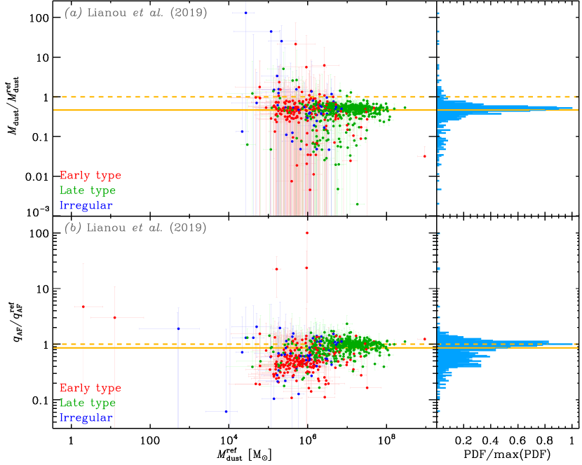
Figure 7: Comparison to Lianou et al. (2019). Same conventions as Fig. 4.

Lianou et al. (2019, hereafter L19) recently used our model, HerBIE, to analyze the DustPedia photometry. There are three main technical differences between our analysis and theirs.

1. They used the implementation of the 2013 version of the THEMIS model (Jones et al., 2013), while we use the revised 2017 version (Jones et al., 2017).

2. They did not profit from the possibility to include ancillary data in the prior (Sect. 3.1).

3. They did not include the remaining sources from the DGS sample.

The comparisons of $M_{\mbox{{\scriptsize dust}}}$ and $q_{\mbox{{\scriptsize AF}}}$ are shown in Fig. 7.

Panel (a) of Fig. 7 shows that their dust mass is about a factor of 2 lower than ours. This can be partly understood in the light of the difference in grain mixtures. Indeed, Jones et al. (2017) revised the THEMIS model by including the more realistic Köhler et al. (2014) optical properties. To fit the same observational constraints, they compensated this update by changing the mantle thickness, as well as the dust-to-gas mass ratio: $M_{\mbox{{\scriptsize dust}}}/M_{\mbox{{\scriptsize H}}}=8.6\times 10^{-3}$ according to Table 2 of Jones et al. (2013) and $M_{\mbox{{\scriptsize dust}}}/M_{\mbox{{\scriptsize H}}}=7.4\times 10^{-3}$ according to Table 1 of Jones et al. (2017). This sole modification explains why a mass derived with the 2013 THEMIS version would be a factor of $\simeq 0.86$ lower than with the 2017 version. However, this does not explain the whole extent of the discrepancy. The comparison of our dust masses with those derived with CIGALE (Sect. 3.3.3) certainly excludes such a large error, on our side. It can be noted that there is also some scatter around the median ratio of $M_{\mbox{{\scriptsize dust}}}/M_{\mbox{{\scriptsize dust}}}^{\mbox{{\scriptsize ref}}}$. A part of this discrepancy can naturally be explained by the fact that several galaxies have a very poor spectral coverage. As demonstrated in Sect. 3.2, the prior becomes dominant in this case. In our case, the prior contains the information provided by the ancillary data, thus helping to reduce the dust parameter range.

Panel (b) of Fig. 7 shows the comparison of $q_{\mbox{{\scriptsize AF}}}$. The two quantities are in good agreement. There is some scatter around the median, for the same reason as mentioned for $M_{\mbox{{\scriptsize dust}}}$. However, the problem with this quantity is the way L19 discuss it. They improperly report the meaning of $q_{\mbox{{\scriptsize AF}}}$ that they call “‘QPAH’” ( L19, Sect. 3, $5^{\textnormal{th}}$ item). They write it represents “the mass fraction of hydrogenated amorphous carbon dust grains with sizes between 0.7 nm and 1.5 nm”, while it actually is the mass fraction of a-C(:H) with sizes between 0.4 nm and 1.5 nm. Furthermore, they claim the Galactic value of this parameter is $7.1\,\%$, while it is $q_{\mbox{{\scriptsize AF}}}^{\mbox{{\scriptsize Gal}}}=18.6\,\%$ for the 2013 version and $q_{\mbox{{\scriptsize AF}}}^{\mbox{{\scriptsize Gal}}}=17.0\,\%$ for the 2017 version. The value of $7.1\,\%$ is the mass fraction of a-C(:H) between 4 Å and 7 Å. Consequently, they mistakenly show that most of the DustPedia sample has a higher fraction of small a-C(:H) than the Milky Way, while it is not the case (cf. Sect. 4.2).

In summary, we are confident that our derived parameters are both more precise and more accurate than L19’s.

4 THE DERIVED DUST EVOLUTION TRENDS

In this section, we present the main dust evolution trends derived from the reference run (Sect. 3.2). These results are displayed as correlations between two inferred parameters, for each source in the sample. Displaying the full posterior PDF of each galaxy as density contours is visually impractical. Instead, we display its extent as a Skewed Uncertainty Ellipse (SUE; Appendix F). SUEs approximately represent the $1\sigma$ contour of the PDF, retaining the information about the correlation and the skewness of the posterior, with a dot at the maximum a posteriori. When discussing parameter values in the text, we often quote the 95$\,\%$ Credible Range (CR_95%), which is the parameter range excluding the $2.5\,\%$ lowest and $2.5\,\%$ highest values of the PDF. We also adopt the following terminology.

• We call Extremelly Low-Metallicity Galaxy (ELMG), a system with $Z\lesssim Z_{\odot}/10$.

• To simplify the discussion, since the heavy-element-to-gas mass ratio, $Z$, is usually called metallicity, we introduce the term dustiness to exclusively denote the dust-to-gas mass ratio:

  $$Z_{\mbox{{\scriptsize dust}}}\equiv\frac{M_{\mbox{{\scriptsize dust}}}}{M_{\mbox{{\scriptsize gas}}}}.$$ (4)

• We denote by specific, quantities per unit stellar mass (similar to sSFR): 1 the specific dust mass is $\textnormal{s}M_{\mbox{{\scriptsize dust}}}\equiv M_{\mbox{{\scriptsize dust}}}/M_{\star}$; 2 the specific gas mass is $\textnormal{s}M_{\mbox{{\scriptsize gas}}}\equiv M_{\mbox{{\scriptsize gas}}}/M_{\star}$.

Note that, in all the displayed relations, the number of objects depends on the availability of the ancillary data (Table 2).

4.1 Evolution of the Total Dust Budget

We first focus on scaling relations involving the total dust mass, $M_{\mbox{{\scriptsize dust}}}$, with respect to the gas and stellar contents, the metallicity and the star formation activity. Casasola et al. (2020a) have explored additional scaling relations, focussing on DustPedia LTGs.

4.1.1 Qualitative Discussion

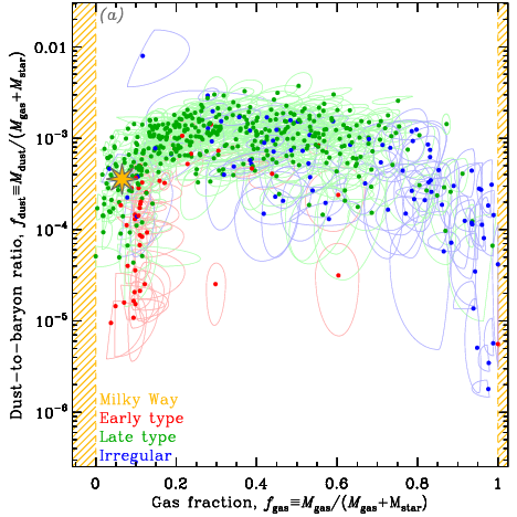
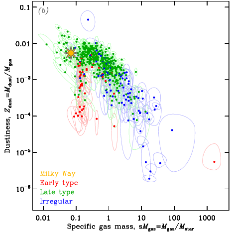
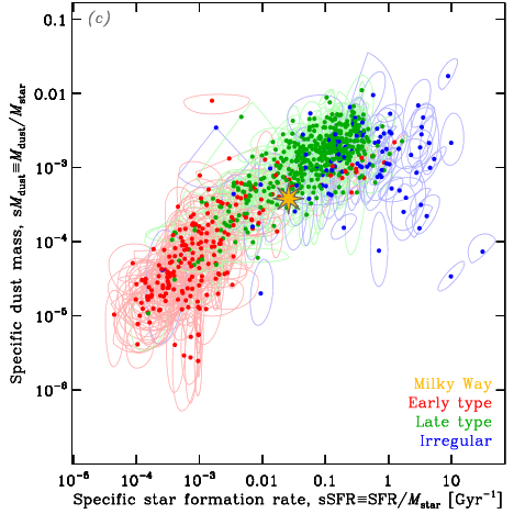
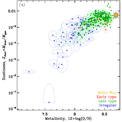
Figure 8: Dust-related scaling relations. In the four panels, the SUEs represent the posterior of each galaxy, using the reference run (Sect. 3.2). The SUEs are color-coded according to the Hubble stage of the object (Sect. 3.3). We show the Milky Way values, as a yellow star, for comparison. We emphasize that, although we are showing different parameters of the same sample, the different panels do not exactly contain the same number of objects (Table 2). In particular, there are fewer reliable metallicity measurements, especially for ETGs.

Fig. 8 presents four important scaling relations. Panel (a) shows the evolution of the dust-to-baryon mass ratio:

$$f_{\mbox{{\scriptsize dust}}}\equiv\frac{M_{\mbox{{\scriptsize dust}}}}{M_{\mbox{{\scriptsize gas}}}+M_{\star}},$$ (5)

as a function of the gas fraction:

$$f_{\mbox{{\scriptsize gas}}}\equiv\frac{M_{\mbox{{\scriptsize gas}}}}{M_{\mbox{{\scriptsize gas}}}+M_{\star}}.$$ (6)

This well-known relation was previously presented by Clark et al. (2015), De Vis et al. (2017a) and Davies et al. (2019). It shows that: 1 at early stages ($f_{\mbox{{\scriptsize gas}}}\gtrsim 0.7$; mainly irregulars), there is a net dust build-up; 2 it then reaches a plateau ($0.2\lesssim f_{\mbox{{\scriptsize gas}}}\lesssim 0.7$; mainly LTGs) where the dust production is counterbalanced by astration; 3 at later stages ($f_{\mbox{{\scriptsize gas}}}\lesssim 0.2$; mainly ETGs), there is a net dust removal. Several sources have peculiar positions relative to the above mentioned trend.

1. The irregular (blue SUE) with $f_{\mbox{{\scriptsize dust}}}\simeq 0.01$ is PGC 166077. It is however technically not an outlier, as $\textnormal{CR}_{95\%}(f_{\mbox{{\scriptsize dust}}})=[1.7\times 10^{-3},2.8\times 10^{-2}]$, overlapping with the rest of the sample.

2. The two ETGs (red SUEs) with a low $f_{\mbox{{\scriptsize dust}}}$, at $f_{\mbox{{\scriptsize gas}}}\simeq 0.3$ and $f_{\mbox{{\scriptsize gas}}}\simeq 0.6$, are NGC 5355 and NGC 4322, respectively. For NGC 4322, $\textnormal{CR}_{95\%}(f_{\mbox{{\scriptsize dust}}})=[1.2\times 10^{-6},1.4\times 10^{-4}]$, marginally overlapping with the rest of the sample. For NGC 5355, however, $\textnormal{CR}_{95\%}(f_{\mbox{{\scriptsize dust}}})=[2.7\times 10^{-6},6.8\times 10^{-5}]$, making it a true outlier.

3. The ETG (red SUE) with $f_{\mbox{{\scriptsize gas}}}\simeq 1$ is ESO 351–030. It is the Sculptor dwarf elliptical galaxy. This is not an outlier to the relation, but it indisputably lies outside of its group.

Panel (b) of Fig. 8 presents the relation between the specific gas mass, and the dustiness. Such a relation was previously presented by Cortese et al. (2012), Clark et al. (2015) and De Vis et al. (2017a). There is a clear negative correlation between these two quantities, showing that when a galaxy evolves, its ISM gets progressively enriched in dust and its gas content gets converted to stars. There is one notable feature deviating from this main sequence: a vertical branch at $\textnormal{s}M_{\mbox{{\scriptsize gas}}}\simeq 0.1$, exhibiting a systematically lower dustiness. This branch is mostly populated by ETGs and contains most of the ETGs of the relation. We will discuss the likely origin of this branch in Sect. 4.1.2. Finally, the peculiar sources of panel (a) logically stand out in this panel too.

1. PGC 166077 is the blue SUE at $Z_{\mbox{{\scriptsize dust}}}\simeq 0.05$. It is not a clear outlier, as $\textnormal{CR}_{95\%}(Z_{\mbox{{\scriptsize dust}}})=[0.01,0.13]$.

2. NGC 5355 and NGC 4322 are the red SUEs at $\textnormal{s}M_{\mbox{{\scriptsize gas}}}\simeq 0.4$ and $\textnormal{s}M_{\mbox{{\scriptsize gas}}}\simeq 1.5$, respectively.

3. The bottom red SUE, at $\textnormal{s}M_{\mbox{{\scriptsize gas}}}\simeq 1600$, is ESO 351-030.

Panel (c) of Fig. 8 shows the relation between the specific dust mass and the specific star formation rate, sSFR. This relation was previously presented by Rémy-Ruyer et al. (2015) and De Vis et al. (2017a). It was also discussed in Cortese et al. (2012) with sSFR replaced by its proxy NUV-r. In the same way, but on resolved 140-pc scales, it was shown in M 31 by Viaene et al. (2014). There is a clear positive correlation between the two quantities. The different galaxy types are grouped in distinct locations: 1 ETGs are clustered around $10^{-4}\lesssim\textnormal{sSFR}\lesssim 0.01\;\textnormal{Gyr}^{-1}$; 2 LTGs are clustered around $0.01\lesssim\textnormal{sSFR}\lesssim 1\;\textnormal{Gyr}^{-1}$; 3 Irregulars tend to lie around $0.1\lesssim\textnormal{sSFR}\lesssim 10\;\textnormal{Gyr}^{-1}$, but are more scattered than the other types, with a systematically lower $\textnormal{s}M_{\mbox{{\scriptsize dust}}}$ than what the extrapolation of the trend would suggest. This scaling relation provides an interesting approximation to derive the dust content from SFR and $M_{\star}$, two quantities which usually are easy to estimate. In particular, the relation is quasi-linear in the low sSFR regime, with:

$$\frac{M_{\mbox{{\scriptsize dust}}}}{\textnormal{M}_{\odot}}\simeq 7.3_{-6.1}^{+10.4}\times 10^{7}\times\frac{\textnormal{SFR}}{\textnormal{M}_{\odot}/\textnormal{yr}}\;\;\mbox{ for }\;\;\textnormal{sSFR}\lesssim 0.1\;\textnormal{Gyr}^{-1},$$ (7)

with $\textnormal{CR}_{95\%}(M_{\mbox{{\scriptsize dust}}}/\textnormal{SFR})=[0.12,53]\times 10^{7}$ yr.

Panel (d) of Fig. 8 shows the variation of the dustiness as a function of the metallicity (Eq. 1). Such a relation is one of the most common benchmarks for global dust evolution models (cf. Sect. 5), and has been presented by numerous studies (e.g.  Lisenfeld & Ferrara, 1998; James et al., 2002; Draine & Li, 2007; Galliano et al., 2008a; Galametz et al., 2011; Rémy-Ruyer et al., 2014; De Vis et al., 2017b). There is a clear correlation between the two quantities, reflecting the progressive dust enrichment of the ISM, built from heavy elements injected by stars at the end of their lifetime. Few ETGs are present, due to the lack of reliable gas metallicity estimates for these objects. These would occupy the high-metallicity regime. Compared to Rémy-Ruyer et al. (2014), who presented a similar trend for the DGS sources, we notice that a few sources are missing and some metallicities have been updated. This comes from the fact that we have adopted the more robust DGS metallicity reestimates by De Vis et al. (2017b), with published nebular lines and using the PG16_S calibration (Sect. 2.2.2). The lowest metallicity source, at $12+\log(\textnormal{O}/\textnormal{H})\simeq 7.15$, is I Zw 18. The most dust-deficient source of the panel, at $Z_{\mbox{{\scriptsize dust}}}\simeq 1.9\times 10^{-6}$, is UGCA 20. It is a clear outlier to the trend with $\textnormal{CR}_{95\%}(Z_{\mbox{{\scriptsize dust}}})=[1.3\times 10^{-6},3.0\times 10^{-6}]$.

4.1.2 Comparison to X-Ray Luminosities

The ETG outliers, visible in panel (b) of Fig. 8 and discussed in Sect. 4.1.1, are likely due to enhanced dust destruction by thermal sputtering in their hot, X-ray emitting gas (e.g.  Bocchio et al., 2012; Smith et al., 2012), as suggested by De Vis et al. (2017a). We could conceive a reverse causality where it is the low dust abundance that allows a higher fraction of escaping X-ray photons. However, this is unrealistic, as X-ray observations clearly indicate that ETGs are permeated by a coronal gas that is usually not found in later types of galaxies (Mathews & Brighenti, 2003, for a review). In order to support the likeliness of the thermal sputtering scenario, we have compiled X-ray luminosities from the literature (Table 4). Fig. 9 displays the dust-to-stellar mass ratio as a function of the X-ray photon rate per dust grain, $L_{\mbox{{\scriptsize X}}}/M_{\mbox{{\scriptsize dust}}}$, for the 256 galaxies in our sample with published X-ray luminosities. This figure shows a mild negative correlation between the two quantities, consistent with the enhanced dust destruction in X-ray-bright galaxies. ETGs clearly lie in the bottom right quadrant of this figure. It is reminiscent of Figure 10 in Smith et al. (2012), displaying $L_{\mbox{{\scriptsize FIR}}}/L_{\mbox{{\scriptsize B}}}$ as a function of $L_{\mbox{{\scriptsize X}}}/L_{\mbox{{\scriptsize B}}}$.

We note there is however a significant intrinsic scatter in this relation. This could be due to the fact that most of the studies listed in Table 4 quote a total X-ray luminosity, including both: 1 point sources (AGNs, binary systems); and 2 the diffuse thermal emission that is sole relevant to our case. In addition, the spectral range used to compute the X-ray luminosity varies from one instrument to the other (Table 4), leading to systematic differences. Nonetheless, accounting for these differences, which is beyond the scope of this paper, would likely not change the plausibility that dust grains are significantly depleted in ETGs due to thermal sputtering.

Table 4: X-ray luminosity references. The total number of sources (last line) is fewer than the sum of each sample size (last column). This is because the same sources were observed by different instruments. When it is the case, we keep the most recent estimate.

Bibliographic	Telescope	Range	Size
reference		[keV]
Fabbiano et al. (1992)	Einstein	$0.2-4$	172
Brinkmann et al. (1994)	ROSAT	$0.1-2.4$	7
O’Sullivan et al. (2001)	ROSAT	$0.1-17$	83
Tajer et al. (2005)	ROSAT	$0.1-2$	10
Cappi et al. (2006)	XMM	$0.2-10$	16
David et al. (2006)	Chandra	$0.5-2$	8
Diehl & Statler (2007)	Chandra	$0.3-5$	7
Rosa González et al. (2009)	XMM	$0.5-2$	1
González-Martín et al. (2009)	Chandra	$0.5-10$	30
Akylas & Georgantopoulos (2009)	XMM	$2-10$	19
Grier et al. (2011)	Chandra	$0.3-8$	29
Brightman & Nandra (2011)	XMM	$2-10$	37
Liu (2011)	Chandra	$0.3-8$	147
Kim et al. (2019)	Chandra	$0.5-5$	12
Total			256

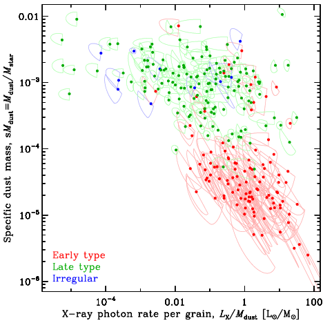
Figure 9: Relation of dust mass to X-ray luminosity. This figure shows the variation of the dust-to-stellar mass ratio as a function of the X-ray photon rate per dust grain, for the sample of Table 4. This is a subset of the reference run (Sect. 3.2). The color convention is similar to Fig. 8. The Bayesian correlation coefficient of this relation is $\rho=-0.596_{-0.015}^{+0.017}$, with $\textnormal{CR}_{95\%}(\rho)=[-0.62,-0.56]$.

4.1.3 On the variation of the Dust-to-Metal Mass Ratio

Panel (d) of Fig. 8 shows that the dustiness-metallicity relation is non-linear. Rémy-Ruyer et al. (2014) first argued, relying on insights from the models of Asano et al. (2013) and Zhukovska (2014), that such a trend was the result of different dust production regimes: 1 at low $12+\log(\textnormal{O}/\textnormal{H})$, dust production is dominated by condensation in type II Supernova (SN) ejecta, with a low yield; 2 around a critical metallicity of $12+\log(\textnormal{O}/\textnormal{H})\simeq 8$, grain growth in the ISM becomes dominant, causing a rapid increase of $Z_{\mbox{{\scriptsize dust}}}$; 3 at high $12+\log(\textnormal{O}/\textnormal{H})$, the dust production is dominated by grain growth in the ISM, with a yield about two orders of magnitude higher than SN ii, and is counterbalanced by SN ii blast wave dust destruction. Rémy-Ruyer et al. (2014) argued that the intrinsic scatter of the relation, which could not be explained by SED fitting uncertainties, was due to the fact that each galaxy has a particular Star Formation History (SFH). We will explore this aspect in Sect. 5. In the following paragraphs, we discuss the different biases that could have induced an artificial non-linearity in our empirical trend.

Comparison to DLAs.

Fig. 10 shows the evolution of the dust-to-metal mass ratio (DTM) as a function of metallicity. It is another way to look at the data in panel (d) of Fig. 8. A constant DTM corresponds to a linear dustiness-metallicity trend. The SUEs in Fig. 10 are not consistent with a constant DTM (horizontal yellow line). However, there are reports in the literature of objects exhibiting an approximately constant DTM, down to very low metallicities: Damped Lyman-$\alpha$ Absorbers (DLA). We have overlaid the DLA sample of De Cia et al. (2016). These measures are performed in absorption on redshifted systems, along the sightline of distant quasars. The metallicity and DTM are derived from a combination of atomic lines of volatile and refractory elements. We can see that the DLA DTMs vary significantly less than in our nearby galaxy sample. Such an evolutionary behaviour requires a high SN-dust condensation efficiency coupled to a weak grain growth rate in the ISM (e.g.  De Vis et al., 2017b). Alternatively, the DLA estimates could be biased. It is indeed not impossible that the hydrogen column density of most DLAs includes dust- and element-free circumgalactic clouds in the same velocity range. It would result in a typical solar metallicity object appearing to have a solar DTM, and at the same time, an artificially lower metallicity, diluted by the additional pristine gas along the line of sight.

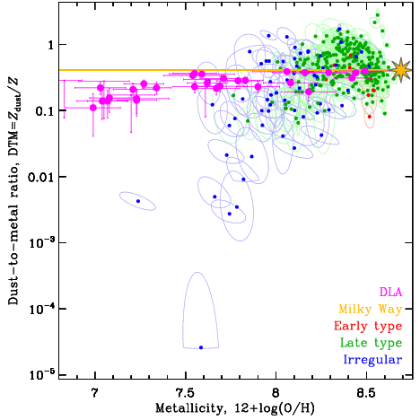
Figure 10: Comparison to DLAs. This figure shows the relation between the metallicity and the dust-to-metal mass ratio, for the reference run (Sect. 3.2). This figure is very similar to panel (d) of Fig. 8: the only difference is that the $y$-axis has been divided by $Z$ (related to the $x$-axis through Eq. 1). We have overlaid in magenta the DLA measures from Table 6 of De Cia et al. (2016). The horizontal yellow line corresponds to the Galactic dust-to-metal mass ratio. The Bayesian correlation coefficient of the nearby galaxy sample is $\rho=0.636_{-0.023}^{+0.021}$, with $\textnormal{CR}_{95\%}(\rho)=[0.59,0.68]$.

Accounting for the Gas Halo.

The contamination of the gas mass estimate by external, dust- and element-poor gas is also a potential issue for our nearby galaxy sample. This is particularly important for low-metallicity, dwarf galaxies, where the IR-emitting region is usually small compared to the whole H i halo (e.g.  Walter et al., 2007; Begum et al., 2008). For instance, Draine et al. (2007) hinted that the trend between $Z$ and $Z_{\mbox{{\scriptsize dust}}}$ was close to linear, when the gas mass used to estimate $Z_{\mbox{{\scriptsize dust}}}$ was integrated in the same region as the dust mass. They only had 9 galaxies below $12+\log(\textnormal{O}/\textnormal{H})<8.1$. We have addressed this issue by adopting the interferometric [H i]${}_{21\,\textnormal{cm}}$ observations of 20 of the lowest metallicity galaxies in our sample, including the lowest metallicity system, I Zw 18 (Roychowdhury et al., in prep.; Sect. 2.2.3). We have integrated the gas mass within the photometric aperture for these 20 objects. I Zw 18 still lies two orders of magnitude below the Galactic DTM, despite this correction. On the contrary, it is possible that the DTM of UGCA 20, the lowest SUE in Fig. 10, has been underestimated, as it has not been resolved in H i. We have to admit that there is still room for improvement as several of the ELMGs are barely resolved in the IR. Thus, although we corrected for a large fraction of the H i halo, there might still be residual gas not associated with the star forming region within our aperture. We might therefore be underestimating the dustiness of our ELMGs. This will have consequences in Sect. 5. The amplitude of this underestimation is not quantifiable as these sources are not resolved in the far-IR. It is however difficult to imagine that there would still be $99\,\%$ of gas not associated with IR emission within our aperture. Indeed, for the most extreme case, I Zw 18, our aperture is only 1.5 times the optical radius (Rémy-Ruyer et al., 2013), which should be comparable to the IR radius. The overall rising DTM with $12+\log(\textnormal{O}/\textnormal{H})$ of Fig. 10 is therefore unlikely due to an improper correction of the H i envelopes of ELMGs.

Variation of the Grain Opacities.

We have noted in Sect. 3.1.3 that our dust mass estimates depend on the rather arbitrary grain opacity we have adopted. This grain opacity has been designed to account for the emission, extinction and depletions of the diffuse Galactic ISM (cf. Sect. 3.1.1). A systematic variation of the overall grain opacity with metallicity could change the slope of the trend in Fig. 10. In order to move I Zw 18 up to the Galactic DTM, we would need to adopt a grain emissivity diminished by about two orders of magnitude. Qualitatively, the ISM of an ELMG, such as I Zw 18, is (e.g.  Cormier et al., 2019): 1 permeated by hard UV photons; 2 very clumpy with a low cloud filling factor. With more UV photons to evaporate the mantles and less clouds to grow them back, we could assume that the grains in such a system would be reduced to their cores (cf. Figure 16 of Jones et al., 2013). Demantled, crystalline, compact grains are indeed among the least emissive grains. However, to our knowledge, there are no interstellar dust analogs having a far-IR opacity two orders of magnitude lower than those used in the THEMIS model. The Draine & Li (2007) mixture, which resembles compact bare grains, is only a factor of $\simeq 2$ less emissive than THEMIS (e.g. Figure 4 of Galliano et al., 2018). We could also imagine that the composition of the dust mixture itself changes. In particular, the fraction of silicates could be higher in ELMGs, as C/O and O/H are correlated (Garnett et al., 1995). This would have a limited effect, since: 1 a decrease of the large a-C(:H) abundance by $50\,\%$ would decrease the global emissivity of THEMIS in the SPIRE bands by $15-30\,\%$; 2 a variation of the forsterite-to-enstatite ratio would change the emissivity by less than $30\,\%$. It is therefore very unlikely that the dependence of DTM with metallicity is artificially induced by our grain opacity assumption.

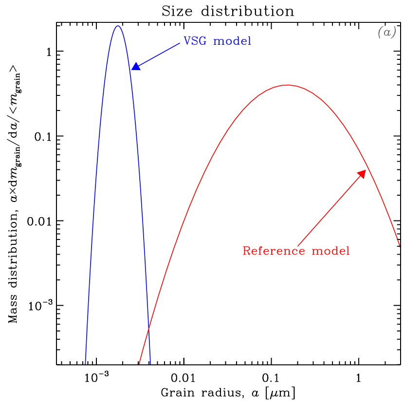
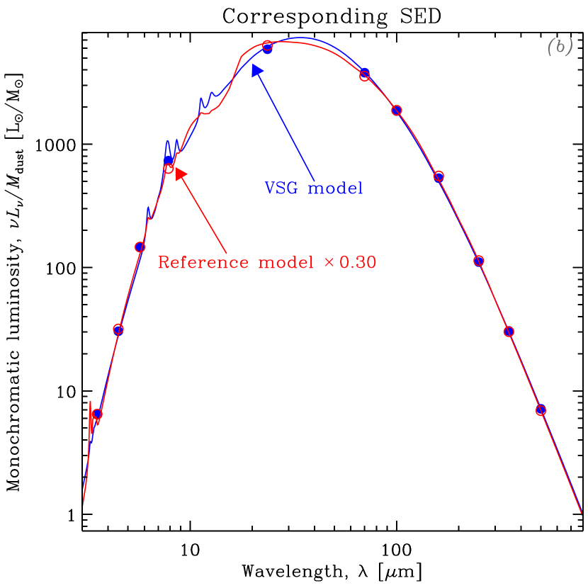
Figure 11: Demonstration of a VSG-dominated SED. Panel (a) shows the size distribution of the two models we are comparing here: the reference model in red, which is simply the THEMIS model, with the small grains scaled down to mimic the SED of a typical ELMG; and a VSG model, in blue, which is a log-normal size distribution, peaking at $1.5$ nm with a log-width of $0.2$. The optical properties of the VSG model are those of THEMIS, and we have kept the same silicate-to-carbon grain mass ratio. In both cases, the curves represent the size distributions of a-C(:H) and silicates. Panel (b) shows the corresponding SEDs for the two models. The SED of the reference model has been scaled down by a factor of $0.30$, to fit the VSG SED. It means the VSG SED reproduces the reference model with a dust mass $3.33$ times higher. The VSG SED is uniformly illuminated by an ISRF with $U=10$, while the reference model has a distribution of ISRFs with $\langle U\rangle=200$. The blue filled and red empty circles show the synthetic photometry of each model in the IRAC, MIPS1, PACS and SPIRE bands.

Variation of the Size Distribution.

Another factor that could affect the trend of Fig. 10 is that we have fixed the size distribution of the large grains. In principle, relaxing this assumption and allowing the size distribution to be dominated by Very Small Grains (VSG) in low-metallicity sources, would raise the DTM of objects such as I Zw 18. Indeed, VSGs are stochastically heated. They spend most of their time at very low temperatures between successive photon absorptions. Their excursion at $T\gtrsim 20$ K will span only a fraction of their time. A mixture of VSGs would thus appear less emissive than a larger grain at an equilibrium temperature close to the high end of their temperature distribution. We have demonstrated this effect in Fig. 11. We have simulated a VSG-dominated SED mimicking a typical ELMG, peaking around $\lambda\simeq 40\;\mu\textnormal{m}$, and with very weak aromatic feature emission (Fig. 11; panel b; blue curve). The size distribution needed to produce such a SED is made almost exclusively of $a\simeq 1.5$ nm radius grains (Fig. 11; panel a; blue curve). We have fit this synthetic SED with our reference model (Sect. 3.1.2), keeping the large grain size distribution fixed (Fig. 11; panel a; red curve), but varying the ISRF distribution. This model reproduces very well the photometric fluxes (Fig. 11; panel b; red circles), but requires a total dust mass a factor of $\simeq 3$ lower than the VSG model. This effect goes in the right direction but is not enough to explain the 2 orders of magnitude required to account for a constant DTM in Fig. 10. We could further decrease the emissivity of the VSG model by lowering the size of the grains. However, it would result in a SED peaking shortward $\lambda\simeq 30\;\mu\textnormal{m}$, inconsistent with our observations. Finally, VSG-dominated ELMGs would not be in agreement with theoretical dust size distribution evolution models (e.g.  Hou et al., 2017; Hirashita & Aoyama, 2019; Aoyama et al., 2020). At early stages, these models predict the ISM being populated of large grains. The reason is that the dust production at these stages is thought to be dominated by SN-ii-condensed dust, and grains condensed in core-collapse SN ejecta are essentially large as the small ones are kinetically sputtered (e.g.  Nozawa et al., 2006).

Very Cold Dust.

A significant fraction of the dust mass could have been overlooked, hidden in the form of very cold dust ($T_{\mbox{{\scriptsize dust}}}\lesssim 10$ K). The emission of this component would manifest as a weakly emissive continuum at submm wavelengths, that we have not accounted for. Very cold dust has been invoked to explain the submm excess in dwarf galaxies (cf. Sect. 3.1.3). It could thus be invoked to flatten our dust-to-metal mass ratio trend, in principle. However, while the excess has been reported by numerous studies, predominantly in dwarf galaxies (e.g.  Galliano et al., 2003, 2005; Dumke et al., 2004; Bendo et al., 2006; Galametz et al., 2009; Bot et al., 2010), very cold dust does not appear as one of its viable explanations. Indeed, to reach such a low temperature, very cold dust should be shielded from the general ISRF in massive dense clumps. In the LMC, Galliano et al. (2011) showed that the excess emission at 10 pc scale was diffuse and negatively correlated with the gas surface density, inconsistent with the picture of a few dense clumps. Similarly, Galametz et al. (2014) and Hunt et al. (2015) showed that this excess was more prominent in the outskirts of late-type disk galaxies, where the medium is less dense. In addition, other realistic physical processes to explain this excess have been proposed (Meny et al., 2007; Draine & Hensley, 2012). Dust analogs also exhibit a flatter submm slope that could partly account for this excess (Demyk et al., 2017a). More qualitatively, it is difficult to conceive of the presence of massive dense clumps in ELMGs, where the dust-poor ISM is permeated by intense UV photons from the young stellar populations that are forming. In addition, this dust would likely be associated with dense gas that we have not accounted for, limiting its impact on the estimated dustiness.

Systematic Uncertainty on the ELMG’s DTM.

Overall, it appears that none of our model assumptions could be demonstrated to be responsible for artificially inducing the observed variation of the DTM. The trend of Fig. 10, for nearby galaxies, is therefore likely real. It is however possible that the dustiness of the ELMGs has been underestimated. We can quote a rough systematic uncertainty for an object such as I Zw 18, the following way.

• Since the H i aperture is a factor of $\simeq 1.5$ times the optical radius, $Z_{\mbox{{\scriptsize dust}}}$ might be underestimated by a factor at most $\simeq 1.5^{2}=2.25$.

• We have discussed that the grain opacity could have been overestimated by a factor of $\simeq 2$. The systematic uncertainty on $Z_{\mbox{{\scriptsize dust}}}$ is thus at most a factor of $\simeq 2$.

• We have discussed that our grain size distribution assumption could lead to an underestimate of $Z_{\mbox{{\scriptsize dust}}}$ by a factor of at most $\simeq 3$.

Overall, we can consider that the dustiness of ELMGs could have been underestimated by a factor of $\simeq\sqrt{2.25^{2}+2^{2}+3^{2}}=4.25$.

4.2 Evolution of the Aromatic Feature Emitters

We now focus our discussion on another important dust parameter, the mass fraction of aromatic feature emitting grains, $q_{\mbox{{\scriptsize AF}}}$ (Sect. 3.1.1). Note that, in the THEMIS model, all grains are either pure a-C(:H) or a-C(:H)-coated. All of them therefore potentially carry aromatic features. However, only the smallest ones ($a\lesssim 10$ nm) will fluctuate to high enough temperatures ($T\gtrsim 300$ K) to emit these features. Finally, we remind the reader that, assuming aromatic features are carried by PAHs, $q_{\mbox{{\scriptsize AF}}}$ is formally equivalent to $\simeq 2.2\times q_{\mbox{{\scriptsize PAH}}}$ (Sect. 3.1.1).

4.2.1 The Competing Small a-C(:H) Evolution Scenarios

The strong spatial variability of the aromatic feature strength has been known for several decades. Dramatic variations have been observed within Galactic and Magellanic H ii regions (e.g.  Boulanger et al., 1998; Madden et al., 2006; Galametz et al., 2013), as well as among nearby galaxies (e.g. Galliano et al., 2003, 2005; Engelbracht et al., 2005; Madden et al., 2006). The following scenarios have been proposed.

Photodestruction.

The aromatic feature strength appears to be negatively correlated with the presence of intense/hard UV fields. For instance, Boulanger et al. (1998) showed that their strength in Galactic PDRs is decreasing when the intensity of the ISRF is increasing. Madden et al. (2006) showed that their strength, within Galactic and Magellanic regions and within nearby galaxies, is negatively correlated with [Ne iii]${}_{15.56\mu\textnormal{m}}$/[Ne ii]${}_{12.81\mu\textnormal{m}}$, an ISRF hardness indicator. Numerous studies confirmed these trends, showing the depletion of aromatic features around massive stars, as a result of the photodissociation and photosublimation of small a-C(:H). At the same time, it was also shown that the aromatic feature strength is empirically correlated with metallicity. This is clear in nearby galaxies, as a whole (e.g.  Engelbracht et al., 2005; Madden et al., 2006), as well as within extragalactic H ii regions (e.g.  Gordon et al., 2008; Khramtsova et al., 2013). This correlation is not inconsistent with photodestruction, as most low-metallicity galaxies detected at IR wavelengths to date are actively forming stars. Their ISM, less opaque due to a lower $Z_{\mbox{{\scriptsize dust}}}$, is permeated by an intense UV field, potentially destroying small a-C(:H) on wider scales. It is also consistent with the increasing strength of the 2175 Å bump with metallicity, comparing sightlines in the Small Magellanic Cloud (SMC), LMC and Milky Way (e.g.  Gordon et al., 2003). The extinction bump is indeed thought to be carried by small carbon grains with aromatic bonds (Joblin et al., 1992).

Inhibited formation.

Alternatively, several studies have explored the possibility that small a-C(:H) are less efficiently formed at low-metallicity. Galliano et al. (2008a) showed that, assuming small a-C(:H) are formed from the carbon produced by AGB stars (on timescales of $\simeq 400$ Myr) and the rest of the grains are mostly made out of the elements produced by massive stars (on timescales of $\simeq 10$ Myr), the aromatic feature emitters are under-abundant at early stages of galaxy evolution. Another scenario, developed by Seok et al. (2014), reproduces the trend of aromatic feature strength with metallicity, assuming small a-C(:H) are the product of the shattering of larger carbon grains (see also Rau et al., 2019; Hirashita & Murga, 2020). Finally, Greenberg et al. (2000) have proposed that aromatic feature carriers could form on grain surfaces in molecular clouds and be photoprocessed in the diffuse ISM. Sandstrom et al. (2010) and Chastenet et al. (2019) show that the spatial distribution of $q_{\mbox{{\scriptsize PAH}}}$ in the Magellanic clouds is consistent with this scenario. This process would also explain the fact that these grains are under-abundant in ELMGs, as the molecular gas fraction rises with metallicity.

4.2.2 Empirical Correlations within Our Sample

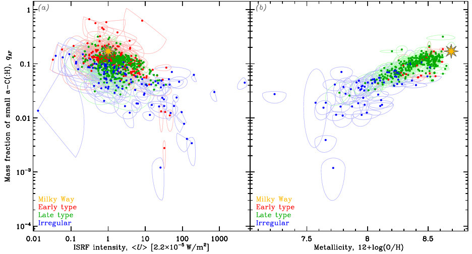
Figure 12: Evolution of small a-C(:H) grains. The SUEs are color-coded according to the type of galaxy (cf. Sect. 3.3). The Milky Way is shown as a yellow star. There are fewer objects with metallicity measurements (376; Table 2), especially among ETGs (panel b).

The different processes we have just listed are not exclusive and could very well compete within the ISM. It is however important to understand which one controls the overall abundance of small a-C(:H), at galaxy-wide scales.

Fig. 12 shows $q_{\mbox{{\scriptsize AF}}}$ as a function of the average starlight intensity, $\langle U\rangle$ (Sect. 3.1.2), and metallicity, in our sample. Similar relations were previously shown by Draine et al. (2007), Galliano et al. (2008a), Khramtsova et al. (2013) and Rémy-Ruyer et al. (2015). The two SUEs at high $\langle U\rangle$ (panel a) are I Zw 18 and SBS 0335-052. Their SEDs indeed peaks around 30 $\mu\textnormal{m}$. However, their $q_{\mbox{{\scriptsize AF}}}$ appear higher than the extrapolation of the general trend, with $\textnormal{CR}_{95\%}(q_{\mbox{{\scriptsize AF}}})=[0.012,0.035]$ for I Zw 18 and $\textnormal{CR}_{95\%}(q_{\mbox{{\scriptsize AF}}})=[0.024,0.064]$ for SBS 0335-052. Mid-IR Spitzer-IRS spectroscopy did not detect aromatic features in these galaxies (Wu et al., 2007; Houck et al., 2004). The true value of $q_{\mbox{{\scriptsize AF}}}$ is likely lower for these two objects. The reason of this overestimation lies in the difficulty to estimate aromatic feature strengths solely with broadband fluxes, when the feature-to-continuum ratio is weak. Indeed, in the weak aromatic feature regime, $q_{\mbox{{\scriptsize AF}}}$ is biased by the color of the mid-IR continuum (cf. Figure 1 of Galliano et al., 2008a).

Overall, we find clear correlations in both panels of Fig. 12, consistent with past studies. However, the relation appears more scattered with $\langle U\rangle$, than with $12+\log(\textnormal{O}/\textnormal{H})$. The correlation coefficient of panel (a) is only $\rho=-0.434_{-0.028}^{+0.038}$ with $\textnormal{CR}_{95\%}(\rho)=[-0.49,-0.35]$, while it is $\rho=0.762_{-0.030}^{+0.018}$ with $\textnormal{CR}_{95\%}(\rho)=[0.70,0.79]$ for panel (b). We could argue that panel (b) of Fig. 12 contains only the 376 sources with metallicity measurements (Table 2), while panel (a) contains the 798 sources with photometric fluxes, including very noisy ETG SEDs. If we consider only the subsample of panel (a) with metallicity measurements, the correlation coefficient does not significantly improve: $\rho=-0.486_{-0.026}^{+0.034}$ with $\textnormal{CR}_{95\%}(\rho)=[-0.54,-0.42]$. If we also exclude the two biased estimates of I Zw 18 and SBS 0335-052, the correlation coefficients do not change much: $\rho=-0.432_{-0.029}^{+0.040}$ with $\textnormal{CR}_{95\%}(\rho)=[-0.49,-0.35]$ for panel (a) and $\rho=0.768_{-0.031}^{+0.018}$ with $\textnormal{CR}_{95\%}(\rho)=[0.70,0.80]$ for panel (b).

We could also question the accuracy of $\langle U\rangle$ as an ISRF tracer. Indeed, $\langle U\rangle$ is a mass-averaged ISRF intensity, giving a large weight to the coldest regions within the beam. Rémy-Ruyer et al. (2015) and Nersesian et al. (2019) used sSFR, which is luminosity weighted, in place of $\langle U\rangle$ and found a good negative correlation with $q_{\mbox{{\scriptsize PAH}}}$ and $q_{\mbox{{\scriptsize AF}}}$, respectively. In our sample, the correlation coefficient between $\ln q_{\mbox{{\scriptsize AF}}}$ and $\ln\textnormal{sSFR}$ is not improved: $\rho=-0.488_{-0.024}^{+0.028}$ with $\textnormal{CR}_{95\%}(\rho)=[-0.53,-0.43]$.

Therefore, it appears that $q_{\mbox{{\scriptsize AF}}}$ correlates much more robustly with metallicity than ISRF indicators, in our sample. This result is worth noting, especially since several studies focussing on a narrower metallicity range concluded the opposite (e.g.  Gordon et al., 2008; Wu et al., 2011). It probably relies on the fact the metallicities we have adopted (Sect. 2.2.2) correspond to well-sampled galaxy averages, while in the past a single metallicity, often central, was available and may have not been representative of the entire galaxy. This result suggests that photodestruction, although real at the scale of star-forming regions, might not be the dominant mechanism at galaxy-wide scales and that one needs to invoke one of the inhibited formation processes discussed in Sect. 4.2.1.

4.3 Approximate Analytical Metallicity Trends

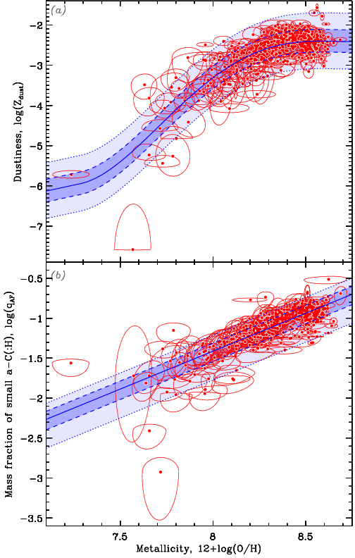
Figure 13: Analytical fit of the scaling relations. The red SUEs show the data of panel (d) of Fig. 8 and panel (b) of Fig. 12. The blue curve in panel (a) shows the analytical fit of Eq. (8) modified by Eq. (9). The blue curve in panel (b) shows the analytical fit of Eq. (10). In both panels, the dashed lines display the envelope encompassing $68\,\%$ of the sources, and the dotted lines, the envelope encompassing $95\,\%$ of the sources. We show here the decimal logarithm of the $Z_{\mbox{{\scriptsize dust}}}$ and $q_{\mbox{{\scriptsize AF}}}$.

It can be interesting to have a simple analytical approximation describing how $Z_{\mbox{{\scriptsize dust}}}$ and $q_{\mbox{{\scriptsize AF}}}$ vary as a function of $12+\log(\textnormal{O/H})$. To that purpose, we have performed polynomial fits of the relations in panel (d) of Fig. 8 and panel (b) of Fig. 12. These fits are displayed in Fig. 13.

A 4${}^{\mbox{{\scriptsize th}}}$ degree polynomial fit of the dustiness-metallicity relation gives, posing $x=12+\log(\textnormal{O/H})$:

$$\log Z_{\mbox{{\scriptsize dust}}}\simeq 11471.808-5669.5959x+1045.9713x^{2}$$ (8)

$$-85.434332x^{3}+2.6078774x^{4}.$$

This equation provides a good fit of our trend, for the metallicity range covered by our sources. However, it gives a rising dustiness trend with decreasing metallicity below I Zw 18. To improve this relation, we can assume that the dustiness will be proportional to $12+\log(\textnormal{O/H})$ at extremelly low-metallicity, as we will show in Sect. 5.3 that dust evolution in this regime is dominated by SN ii production. We therefore modify Eq. (8), as:

$$\log Z_{\mbox{{\scriptsize dust}}}\simeq-13.230+x\;\;\;\mbox{ for }x<7.3.$$ (9)

This fit splits our data in two equal size samples above and below. To quantify its uncertainty, we can compute the envelopes corresponding to encompassing $68\,\%$ and $95\,\%$ of the sources, adding $[-0.27,+0.29]$ and $[-0.68,+0.70]$ respectively to the fit of $\log Z_{\mbox{{\scriptsize dust}}}$.

In the case of $q_{\mbox{{\scriptsize AF}}}$, a 1${}^{\mbox{{\scriptsize st}}}$ degree polynomial gives a satisfactory fit as a function of $12+\log(\textnormal{O/H})$:

$$\log q_{\mbox{{\scriptsize AF}}}\simeq-9.001+0.9486x.$$ (10)

Its $68\,\%$ and $95\,\%$ envelopes are obtained adding $[-0.13,+0.10]$ and $[-0.36,+0.20]$, respectively.

5 EMPIRICAL QUANTIFICATION OF KEY DUST EVOLUTION PROCESSES

We now analyze the trends of Fig. 8, in a more quantitative way, with the help of a grain evolution model. The goal here is two-fold: 1 by fitting theoretical tracks to our sample, we intend to test if it is possible to account for the variation of the main galaxy parameters, with only a few evolutionary processes; 2 we aim to give a self-consistent empirical quantification of the main ad hoc tuning parameters controlling these evolutionary processes.

5.1 The Cosmic Dust Evolution Model

Cosmic dust evolution models compute the variation of the dust content of a galaxy as a function of time. Dwek & Scalo (1980) presented the first model of this kind, developed as an extension of models computing the elemental enrichment of the ISM (Audouze & Tinsley, 1976, for an early review). Subsequent attempts, with various degrees of complexity, followed (e.g.  Dwek, 1998; Lisenfeld & Ferrara, 1998; Hirashita, 1999; Morgan & Edmunds, 2003; Inoue, 2003; Dwek et al., 2007; Galliano et al., 2008a; Calura et al., 2008; Valiante et al., 2009; Mattsson & Andersen, 2012; Asano et al., 2013; Zhukovska, 2014; Feldmann, 2015; De Looze et al., 2020; Nanni et al., 2020). Recently, such models have been used to post-process numerical simulations in order to provide a more comprehensive understanding of galaxy evolution (e.g.  Aoyama et al., 2017).

5.1.1 Model Hypothesis

We adopt the one-zone dust evolution model of Rowlands et al. (2014) updated by De Vis et al. (2017b). It solves the coupled differential equations accounting for the time evolution of the mass of the four following quantities.

Stars

are made out of the gas, which is partially returned to the ISM at the end of their lifetime. The model tracks their evolution as a function of their mass, which determines their lifetime and their elemental and dust yields. The role of this component therefore relies greatly on the form of the assumed IMF (e.g.  Salpeter, 1955; Chabrier, 2003).

Gas

is depleted by astration and outflow, and is replenished by stellar feedback and by inflow of metal- and dust-free gas.

Heavy elements

are injected in the ISM by stars at the end of their lifetime. A fraction of them is recycled into stars through astration and lost via outflow.

Dust

is produced by three main processes: 1 condensation in Low- and Intemediate-Mass Star (LIMS) ejecta ($m_{\star}<8\;\textnormal{M}_{\odot}$); 2 condensation in SN ii ejecta ($m_{\star}\geq 8\;\textnormal{M}_{\odot}$); 3 grain growth in the ISM, by accretion of elements onto grain seeds. Dust is removed from the ISM by: 1 destruction by SN ii blast waves; 2 outflow; 3 astration.

The drivers of the evolution of these quantities are: 1 the assumed SFH (i.e. the SFR as a function of time); 2 the assumed inflow and outflow rates.

5.1.2 The Tuning Parameters

The efficiencies of individual dust evolution processes are poorly known (see reviews by Dwek, 2005; Draine, 2009; Jones, 2016a, b, c; Galliano et al., 2018). From a theoretical point of view, these efficiencies depend on the most elusive detailed microscopic dust properties: chemical constitution, structure (crystalline, amorphous, aggregate, etc.) and size. Consequently, theoretical estimates usually span several orders of magnitude. From an observational point of view, unambiguous constraints of the evolution rates are also problematic, because it is nearly impossible to isolate a dust source or sink in a telescope beam. Dust evolution models therefore use simple parametric efficiencies controlled by tuning parameters.

Dust condensation in SN-II ejecta.

Dust formed by massive stars ($m_{\star}\geq 8\;\textnormal{M}_{\odot}$) is thought to dominate the dust production at early stages, below the critical metallicity (cf. Sect. 4.1.3). The dust evolution model we are using assumes the theoretical dust yields, $m_{\mbox{{\scriptsize dust}}}^{\mbox{{\scriptsize SN}}}$, of Todini & Ferrara (2001), modified by a general tuning parameter, $\delta_{\mbox{{\scriptsize SN}}}$ (Table 5). These dust yields can also be integrated over the IMF, $\phi(m_{\star})$:

$$\langle Y_{\mbox{{\scriptsize SN}}}\rangle\equiv\frac{\displaystyle\int_{8\;\textnormal{M}_{\odot}}^{40\;\textnormal{M}_{\odot}}\phi(m_{\star})\times m_{\mbox{{\scriptsize dust}}}^{\mbox{{\scriptsize SN}}}(m_{\star})\,\textnormal{d}m_{\star}}{\displaystyle\int_{8\;\textnormal{M}_{\odot}}^{40\;\textnormal{M}_{\odot}}\phi(m_{\star})\,\textnormal{d}m_{\star}},$$ (11)

to provide a single averaged dust yield per SN ii. For both Salpeter (1955) and Chabrier (2003) IMFs, it is: $\langle Y_{\mbox{{\scriptsize SN}}}\rangle\simeq 0.35\times\delta_{\mbox{{\scriptsize SN}}}\;\textnormal{M}_{\odot}/\textnormal{SN}$. The dust condensation timescale, $\tau_{\mbox{{\scriptsize cond}}}$, can be expressed as a function of the SN ii rate, $R_{\mbox{{\scriptsize SN}}}$:

$$\frac{1}{\tau_{\mbox{{\scriptsize cond}}}(t)}=\langle Y_{\mbox{{\scriptsize SN}}}\rangle\frac{R_{\mbox{{\scriptsize SN}}}(t)}{M_{\mbox{{\scriptsize dust}}}(t)}.$$ (12)

Table 5: SN II dust yields. These values are the Todini & Ferrara (2001) yields, compiled by Rowlands et al. (2014). They are multiplied by the tuning parameter $\delta_{\mbox{{\scriptsize SN}}}$, used by De Vis et al. (2017b).

Individual star mass, $m_{\star}$	Dust yield, $m_{\mbox{{\scriptsize dust}}}^{\mbox{{\scriptsize SN}}}$
$8.5\;\textnormal{M}_{\odot}$	$0\;\textnormal{M}_{\odot}\times\delta_{\mbox{{\scriptsize SN}}}$
$9\;\textnormal{M}_{\odot}$	$0.17\;\textnormal{M}_{\odot}\times\delta_{\mbox{{\scriptsize SN}}}$
$12\;\textnormal{M}_{\odot}$	$0.2\;\textnormal{M}_{\odot}\times\delta_{\mbox{{\scriptsize SN}}}$
$15\;\textnormal{M}_{\odot}$	$0.5\;\textnormal{M}_{\odot}\times\delta_{\mbox{{\scriptsize SN}}}$
$20\;\textnormal{M}_{\odot}$	$0.5\;\textnormal{M}_{\odot}\times\delta_{\mbox{{\scriptsize SN}}}$
$22\;\textnormal{M}_{\odot}$	$0.8\;\textnormal{M}_{\odot}\times\delta_{\mbox{{\scriptsize SN}}}$
$25\;\textnormal{M}_{\odot}$	$1.0\;\textnormal{M}_{\odot}\times\delta_{\mbox{{\scriptsize SN}}}$
$30\;\textnormal{M}_{\odot}$	$1.0\;\textnormal{M}_{\odot}\times\delta_{\mbox{{\scriptsize SN}}}$
$35\;\textnormal{M}_{\odot}$	$0.6\;\textnormal{M}_{\odot}\times\delta_{\mbox{{\scriptsize SN}}}$
$40\;\textnormal{M}_{\odot}$	$0.4\;\textnormal{M}_{\odot}\times\delta_{\mbox{{\scriptsize SN}}}$

Grain growth in the ISM.

The dust build-up by accretion of gas atoms onto pre-existing dust seeds is a potentially dominant production process at late stages, above the critical metallicity (Sect. 4.1.3). We adopt the parametrization of Mattsson et al. (2012), where the grain growth timescale, $\tau_{\mbox{{\scriptsize grow}}}$, is parametrized by a tuning parameter, $\epsilon_{\mbox{{\scriptsize grow}}}$:

$$\frac{1}{\tau_{\mbox{{\scriptsize grow}}}(t)}=\epsilon_{\mbox{{\scriptsize grow}}}\frac{\psi(t)}{M_{\mbox{{\scriptsize gas}}}(t)}\left(Z(t)-Z_{\mbox{{\scriptsize dust}}}(t)\right),$$ (13)

where $\psi(t)$ is the SFR as a function of time $t$. This tuning parameter encompasses our uncertainty about grain sizes, sticking coefficients and the fraction of cold clouds where dust growth occurs.

Dust destruction by SN II blast waves.

SN ii shock waves destroy dust by kinetic sputtering and grain-grain collisional vaporization (e.g.  Jones et al., 1994). We adopt the dust destruction timescale, $\tau_{\mbox{{\scriptsize dest}}}$, of Dwek & Scalo (1980):

$$\frac{1}{\tau_{\mbox{{\scriptsize dest}}}(t)}=\frac{m_{\mbox{{\scriptsize gas}}}^{\mbox{{\scriptsize dest}}}R_{\mbox{{\scriptsize SN}}}(t)}{M_{\mbox{{\scriptsize gas}}}(t)},$$ (14)

where $m_{\mbox{{\scriptsize gas}}}^{\mbox{{\scriptsize dest}}}$ is a tuning parameter quantifying the effective mass of ISM swept by a single SN ii blast wave within which all the grains are destroyed.

5.2 Modelling the Evolution of Individual Galaxies

We use the dust evolution model of Sect. 5.1 to fit, for each galaxy: $M_{\mbox{{\scriptsize dust}}}$, $M_{\mbox{{\scriptsize gas}}}$, $M_{\star}$, SFR and $Z$. Dust destruction in X-ray emitting gas is not taken into account in this model. We therefore exclude the ETGs ($T\leq 0$) which would not be consistently fitted (cf. Sect. 4.1.2). The sample we model here contains 556 sources.

5.2.1 The Model Grid

We have generated a large grid of models that we interpolate to find the best evolution tracks for each of our sources. We assume a delayed SFH (Lee et al., 2010):

$$\psi(t)=\psi_{0}\frac{t}{\tau_{\mbox{{\scriptsize SFH}}}}\exp\left(-\frac{t}{\tau_{\mbox{{\scriptsize SFH}}}}\right),$$ (15)

parametrized by the SFH timescale, $\tau_{\mbox{{\scriptsize SFH}}}$, and a scaling factor, $\psi_{0}$. We assume a Salpeter (1955) IMF in order to be consistent with the observed SFR and stellar mass estimates (Sect. 2.2). Exchanges of matter between galaxies and their environment can have a significant role in regulating the global dustiness at all redshifts (e.g.  Jones et al., 2018; Ohyama et al., 2019; Sanders et al., 2020; Burgarella et al., 2020). We account for inflow and outflow, assuming their rates are proportional to SFR: $R_{\mbox{{\scriptsize in/out}}}(t)=\delta_{\mbox{{\scriptsize in/out}}}\times\psi(t)$. Table 6 gives the parameters of our dust evolution model grid. We perform log-log interpolation of this grid in order to estimate the tracks corresponding to any arbitrary combination of parameters.

Table 6: Dust evolution parameter grid. Individual galaxy parameters control the particular SFH of each galaxy. Common dust evolution parameters are fitted to the whole sample, assuming their values are the same for each galaxy. The grid step (4^th column) is logarithmic for all parameters except the time grid. The SFR scale is normalized to the total initial mass of the galaxy, $M_{0}$. All extensive quantities computed by the model are proportional to $M_{0}$, while intensive quantities are independent of $M_{0}$. In practice, we generate a grid for an arbitrary $M_{0}=4\times 10^{10}\;\textnormal{M}_{\odot}$. This parameter cancels out in the process, as we are fitting ratios (Sect. 5.2.2).

Parameter	Notation	Range	Step
Individual galaxy parameters
Age [Gyr]	$t$	$[0.001,15]$	0.15
SF timescale [Gyr]	$\tau_{\mbox{{\scriptsize SFH}}}$	$[0.1,30]$	0.57 (ln)
SFR scale [Gyr-1]	$\psi_{0}/M_{0}$	$[0.0125,12.5]$	0.26 (ln)
Inflow rate / SFR	$\delta_{\mbox{{\scriptsize in}}}$	$[0.05,4]$	0.37 (ln)
Outflow rate / SFR	$\delta_{\mbox{{\scriptsize out}}}$	$[0.05,4]$	0.13 (ln)
Common dust evolution parameters
SN condensation	$\delta_{\mbox{{\scriptsize SN}}}$	$[0.001,1]$	0.37 (ln)
Grain growth	$\epsilon_{\mbox{{\scriptsize grow}}}$	$[100,10000]$	0.17 (ln)
SN dest. [$\textnormal{M}_{\odot}$]	$m_{\mbox{{\scriptsize gas}}}^{\mbox{{\scriptsize dest}}}$	$[50,1500]$	0.34 (ln)

The SFH we have adopted here, to compute the chemical evolution, is different from the SFH used by Nersesian et al. (2019) to model the SEDs and estimate the observed SFR and $M_{\star}$ (cf. Sect. 2.2.1). Ideally, adopting the same SFH would be more consistent. However, adding a second functional form to Eq. (15), accounting for a potential recent burst, would push this model beyond our current computational capabilities, by increasing the number of free parameters. At the same time, the elemental and dust enrichment by this recent burst would probably be negligible. Alternatively, we could have also modelled the SED, using solely Eq. (15). The problem, in this case, is that the use of a single stellar population biases the estimate of $M_{\star}$ (cf. Appendix B.2).

5.2.2 Hierarchical Bayesian Dust Evolution Inference

To constrain our dust evolution model, we consider the posterior inference of our reference run (Sect. 3.2) as a set of observational constraints. We fit the four independent, intensive quantities: $\textnormal{s}M_{\mbox{{\scriptsize dust}}}$, $\textnormal{s}M_{\mbox{{\scriptsize gas}}}$, sSFR and $Z$. The complex PDF, including the intricate parameter correlations, is preserved in this process. We make the restrictive assumption that the three tuning parameters, $\delta_{\mbox{{\scriptsize SN}}}$, $\epsilon_{\mbox{{\scriptsize grow}}}$ and $m_{\mbox{{\scriptsize gas}}}^{\mbox{{\scriptsize dest}}}$ are universal and are therefore identical in every galaxy. Consequently, we assume that the difference between galaxies is solely the result of their particular individual SFH. We vary the age of the galaxy, $t$, the two SFH parameters, $\tau_{\mbox{{\scriptsize SFH}}}$ and $\psi_{0}$, and the inflow and outflow rates, $\delta_{\mbox{{\scriptsize in}}}$ and $\delta_{\mbox{{\scriptsize out}}}$.

On the universality of the tuning parameters.

As we have seen, the three tuning parameters hide effects of the dust constitution, size distribution, fraction of cold clouds, etc. These quantities could vary across different environments. However, as we will show in Sect. 5.3.1, the SN II dust condensation dominates in the low-metallicity regime, while grain growth and SN destruction are important above the critical metallicity. Thus, the parameters that we will constrain are representative of the regime where they dominate the dust budget. Exploring their variation with the environment is probably premature. We will however be able to infer the variation of the timescales across galaxies, from Eqs. (11) – (14). In addition, if we were to infer one set of tuning parameters per galaxy, it would imply that they vary as a function of the galaxy’s global parameters. In order to be consistent, we would then need to implement these variations of the tuning parameters in the dust evolution model, and change their value at each time step, accordingly.

The model prior.

We have built a HB model to infer these parameters. The prior of the five SFH-related parameters is a multivariate Student’s $t$ distribution controlled by hyperparameters, similar to the treatment in HerBIE. We have assumed wide log-normal priors for the three common tuning parameters. These priors are centered at $\ln 0.1$, $\ln 1000$ and $\ln 320\,\textnormal{M}_{\odot}$ with standard-deviations, $0.8$, $0.8$ and $0.4$, for $\delta_{\mbox{{\scriptsize SN}}}$, $\epsilon_{\mbox{{\scriptsize grow}}}$ and $m_{\mbox{{\scriptsize gas}}}^{\mbox{{\scriptsize dest}}}$, respectively. These priors were designed so that their $\pm 3\sigma$ range roughly corresponds to the extent of the values reported in the literature: $1\,\%\lesssim\delta_{\mbox{{\scriptsize SN}}}\lesssim 100\,\%$, $100\lesssim\epsilon_{\mbox{{\scriptsize grow}}}\lesssim 10^{4}$ and $100\,\textnormal{M}_{\odot}\lesssim m_{\mbox{{\scriptsize gas}}}^{\mbox{{\scriptsize dest}}}\lesssim 1000\,\textnormal{M}_{\odot}$. It does not mean that these parameters can not exceed these limits, but it will be a priori improbable. The reason to adopt weakly informative priors is to avoid unrealistic degeneracies. For instance, there is a well-known degeneracy between grain growth and grain destruction (e.g.  Mattsson & Andersen, 2012; De Vis et al., 2017b; De Looze et al., 2020). Indeed, the ratio of the two timescales, $\tau_{\mbox{{\scriptsize dest}}}(t)/\tau_{\mbox{{\scriptsize grow}}}(t)\propto\epsilon_{\mbox{{\scriptsize grow}}}/m_{\mbox{{\scriptsize gas}}}^{\mbox{{\scriptsize dest}}}\times(Z(t)-Z_{\mbox{{\scriptsize dust}}}(t))$ is not constant, but the metallicity dependence is quite mild in the narrow range above the critical metallicity. This is enough to allow the MCMC to explore unrealistically high values of $\epsilon_{\mbox{{\scriptsize grow}}}$ and $m_{\mbox{{\scriptsize gas}}}^{\mbox{{\scriptsize dest}}}$, if we assume a flat prior.

HB run specifications.

Accounting for the missing ancillary data, we have a total of 1913 observational constraints, for our 556 sources. One may note that we are fitting a model with $5\times 556+3=2783$ parameters and $5+5+C_{5}^{2}=20$ hyperparameters. This is not an issue in the Bayesian approach (e.g.  Hogg et al., 2010). Model parameters are rarely completely independent. Furthermore, the hyperprior is the dominant constraint for very scattered parameters (G18). Finally, by sampling the full joint PDF, a Bayesian model clearly delineates the various degeneracies, provided the MCMC has converged towards the stationary posterior. We have run 12 parallel MCMCs, starting from uniformly distributed random initial conditions within the parameter ranges in Table 6, in order to ensure the uniqueness of our posterior. The results discussed below are from a $10^{5}$ length MCMC, removing the first $10^{4}$ steps to account for burn-in. The longest integrated autocorrelation time is 6200.

5.2.3 The Fitted Dust Evolution Tracks

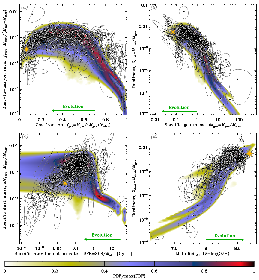
Figure 14: Fitted dust evolution tracks, assuming a Salpeter (1955) IMF. The four panels represent the same quantities as Fig. 8. The black SUEs represent the 556 galaxies of our subsample. The yellow star is the Milky Way. The colored density contours represent the posterior PDF of dust evolution tracks, marginalizing over the individual SFH of each galaxy.

The four panels of Fig. 14 present the same relations as in Fig. 8, for the subsample of 556 sources. The posterior PDF of the dust evolution tracks is displayed as colored density contours, marginalizing over the SFH of individual galaxies.

Qualitative inspection.

At first glance, we can see that the tracks of Fig. 14 reproduce the data quite well. Apart from a few outliers, there are however two notable systematic discrepancies.

1. The $\textnormal{s}M_{\mbox{{\scriptsize dust}}}$-sSFR trend of panel (c) is poorly reproduced. The initial rise of $\textnormal{s}M_{\mbox{{\scriptsize dust}}}$ at $\textnormal{sSFR}\gtrsim 0.3\;\textnormal{Gyr}^{-1}$ undershoots several of the starbursting dwarf galaxies. Overall, this discrepancy is quite mild, as most of the SUEs in this area are less than 2$\sigma$ away from the trend. The recent burst of star formation, that is not accounted for by the chemical evolution model, is likely responsible for the enhanced observed SFR. On the contrary, a starburst occuring in more evolved objects, on the left of this trend, might simply contribute to the general scatter of the relation and go unnoticed. Below $\textnormal{sSFR}\lesssim 0.1\;\textnormal{Gyr}^{-1}$, there is a general decreasing trend of $\textnormal{s}M_{\mbox{{\scriptsize dust}}}$ with decreasing sSFR, but our model is essentially flat. This is the most troublesome discrepancy of our analysis. We will discuss it fully below.

2. In panel (a), several high-gas-fraction sources are undershot by the model, although most of them are only less than 2$\sigma$ away from the tracks. Those are the irregular galaxies around the critical metallicity regime. They are in the stage where the dustiness changes rapidly, due to the increased contribution of grain growth. These outliers can be seen in panel (b), around $\textnormal{s}M_{\mbox{{\scriptsize gas}}}\simeq 10$, in panel (c), around $\textnormal{sSFR}\simeq 3\;\textnormal{Gyr}^{-1}$, and in panel (d), around $12+\log(\textnormal{O/H})\simeq 8$. The model poorly reproduces the rapid dustiness rise around the critical metallicity, in panel (d).

On the $\textnormal{s}M_{\mbox{{\scriptsize dust}}}$-sSFR relation.

The quasi-linear trend of $\textnormal{s}M_{\mbox{{\scriptsize dust}}}$ with sSFR, for $\textnormal{sSFR}\lesssim 0.1\;\textnormal{Gyr}^{-1}$ (panel (c) of Fig. 14), is not accounted for by our model. N20 argue that outflows is responsible for this trend. Indeed, outflow depletes the dust content proportionally to SFR, without affecting the stellar content. It seems like a natural explanation. The outflow rate, $\delta_{\mbox{{\scriptsize out}}}$, is a free parameter in our model. However, it does not produce a linear $\textnormal{s}M_{\mbox{{\scriptsize dust}}}$-sSFR relation. Fig. 15 shows the same data as in panel (c) of Fig. 14. We have overlaid several dust evolution tracks corresponding to our maximum a posteriori parameters, varying $\delta_{\mbox{{\scriptsize out}}}$. This figure is similar to Fig. 6 of N20. We note the following.

1. We can see that no single track can reproduce the trend. It could be a satisfactory explanation if galaxies were rapidly evolving off the main trend, staying only a small fraction of their lifetime on the horizontal branch. However, looking at the top axis of Fig. 15, we realize that a galaxy should spend about half of its lifetime on the horizontal branch. If our model was correct, there should have been, statistically, a significant number of sources deviating from the main trend.

2. The range of $\delta_{\mbox{{\scriptsize out}}}$ values that can account for most of the trend is quite narrow (Fig. 15). It would mean that the outflow has to be precisely regulated. It seems unlikely.

3. If this trend was solely due to outflow, the specific gas mass would follow it closely, which is not the case. This point has also been discussed by Cortese et al. (2012).

In summary, it appears our failure at reproducing the $\textnormal{s}M_{\mbox{{\scriptsize dust}}}$-sSFR relation is rather an incapacity of our model to produce a realistic trend, rather than a fitting issue. As we will see in Sect. 5.3.3, this is not an IMF-related issue. Since the other trends are acceptably reproduced, the problem might lie in the only quantity represented in panel (c) of Fig. 14 not appearing in the other panels: the SFR. Our adopted SFH (Eq. 15) and our inflow and outflow prescriptions might be too simplistic to account for the wealth of data we have here (cf. e.g.  Leja et al., 2019, for a discussion on the limitations of the delayed SFH).

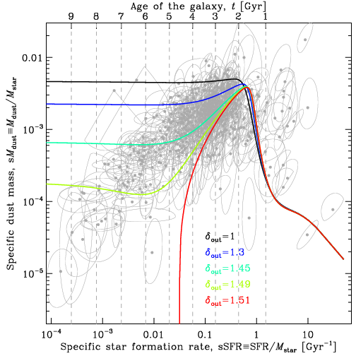
Figure 15: Effect of outflow on the $\textnormal{s}M_{\mbox{{\scriptsize dust}}}$-sSFR relation. The data is identical to panel (c) of Fig. 14. The colored lines represent our dust evolution model. We have fixed all the parameters close to their maximum a posterior values, except the outflow rate, $\delta_{\mbox{{\scriptsize out}}}$: $\tau_{\mbox{{\scriptsize SFH}}}=0.8$ Gyr, $\psi_{0}=40\;\textnormal{M}_{\odot}/\textnormal{yr}$, $\delta_{\mbox{{\scriptsize in}}}=1.0$, $\delta_{\mbox{{\scriptsize SN}}}=0.01$, $\epsilon_{\mbox{{\scriptsize grow}}}=4500$ and $m_{\mbox{{\scriptsize gas}}}^{\mbox{{\scriptsize dest}}}=1200\;\textnormal{M}_{\odot}/\textnormal{SN}$. The different lines correspond to different values of $\delta_{\mbox{{\scriptsize out}}}$. The top axis displays the age of the galaxy corresponding to the particular SFH of the model run. We have used a Salpeter (1955) IMF.

The importance of fitting dust evolution models.

We stress the importance of actually fitting, in a consistent way, dust evolution models, rather than simply performing visual comparisons. Here, we have attempted to fit $M_{\star}$, $M_{\mbox{{\scriptsize gas}}}$, $M_{\mbox{{\scriptsize dust}}}$, Z and SFR for each galaxy. This rigorous process highlights the model limitations. Most past studies have merely overlaid tracks on their data, producing a convincing but inconsistent interpretation. For instance, De Vis et al. (2017b), who used the same dust evolution model as we use, and compared it to a similar sample as ours, were able to produce tracks accounting for most of the observations in the panels (a) and (d) of our Fig. 14. However, two quantities of a given galaxy, such as the dust and stellar masses, were usually explained with different values of the dust evolution parameters, at different ages. On the contrary, our approach allows us to avoid mutually inconsistent explanations of different trends and correlations. Overall, performing a rigorous fit does not help getting better solutions, but it definitely helps avoiding bad ones.

5.3 The Inferred Dust Evolution Parameters

We now discuss the parameters inferred from the fit of Sect. 5.2.3.

5.3.1 Parameter Distribution

The fits of Fig. 14 allow us to infer the common dust evolution tuning parameters, as well as the individual SFH-related parameters (Table 6).

The dust evolution tuning parameters.

The PDF of the three common dust evolution tuning parameters is displayed in Fig. 16. We infer the following values:

• $\langle Y_{\mbox{{\scriptsize SN}}}\rangle\simeq 7.3_{-0.3}^{+0.2}\times 10^{-3}\;\textnormal{M}_{\odot}/\textnormal{SN}$;

• $\epsilon_{\mbox{{\scriptsize grow}}}\simeq 4045_{-354}^{404}$;

• $m_{\mbox{{\scriptsize gas}}}^{\mbox{{\scriptsize dest}}}\simeq 1288_{-8}^{+7}\;\textnormal{M}_{\odot}/\textnormal{SN}$.

The relatively small uncertainties on these parameters reflect the fitting uncertainties. They indicate the values we infer are not ambiguous. However, they do not include the assumption-dependent uncertainties. In particular, the precise value of $\langle Y_{\mbox{{\scriptsize SN}}}\rangle$ relies mainly on our estimate of the dustiness of the few ELMGs in our sample. In Sect. 4.1.3, we have extensively discussed the different systematic effects that could have biased these estimates. If some of these effects are, at some point, proven to be relevant, our inference of $\langle Y_{\mbox{{\scriptsize SN}}}\rangle$ would have to be revised accordingly. To first order, the SN dust yield is proportional to the dustiness of the lowest metallicity objects:

$$\langle Y_{\mbox{{\scriptsize SN}}}\rangle\simeq 0.007\;\textnormal{M}_{\odot}/\textnormal{SN}\times\frac{Z_{\mbox{{\scriptsize dust}}}(\textnormal{I$\;$Zw$\;$18})}{1.9\times 10^{-6}}.$$ (16)

We also notice that $\delta_{\mbox{{\scriptsize SN}}}$ and $m_{\mbox{{\scriptsize gas}}}^{\mbox{{\scriptsize dest}}}$ are peaking at the tail of their prior. It means our data carries a large weight evidence. It also means the values we infer are probably an upper limit for $\delta_{\mbox{{\scriptsize SN}}}$ and a lower limit for $m_{\mbox{{\scriptsize gas}}}^{\mbox{{\scriptsize dest}}}$. Since $m_{\mbox{{\scriptsize gas}}}^{\mbox{{\scriptsize dest}}}$ and $\epsilon_{\mbox{{\scriptsize grow}}}$ are correlated, our inference of $\epsilon_{\mbox{{\scriptsize grow}}}$ is also probably a lower limit. We have estimated in Sect. 4.1.3 that the dustiness of ELMGs could have been underestimated by a factor of at most $\simeq 4.25$, the conservative conclusions we can draw from our analysis are thus that:

• $\langle Y_{\mbox{{\scriptsize SN}}}\rangle\lesssim 0.03\;\textnormal{M}_{\odot}/\textnormal{SN}$;

• $\epsilon_{\mbox{{\scriptsize grow}}}\gtrsim 3000$;

• $m_{\mbox{{\scriptsize gas}}}^{\mbox{{\scriptsize dest}}}\gtrsim 1200\;\textnormal{M}_{\odot}/\textnormal{SN}$.

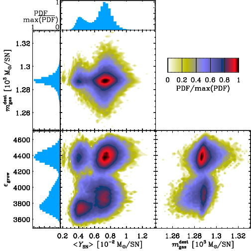
Figure 16: Posterior distribution of the tuning parameters, assuming a Salpeter (1955) IMF. The three central panels with colored contours display the bidimensional posterior PDF of pairs of parameters, marginalizing over all the other ones. The three margin plots show the posterior PDF of each tuning parameter. The PDFs are scaled (divided by their maximum). The displayed ranges encompass every single parameter draw after burn-in.

The SFH-related parameters.

Fig. 17 displays the corner plot of the five parameters controlling the individual SFH of each galaxy. The displayed PDF is the posterior of the parameters of every galaxy. There is a relatively large scatter of these parameters, implying that our different galaxies have different SFHs. Note that the interpolation between models does not produce a perfectly smooth distribution. The edges of our model grid are visible in this corner plot. This does not however impact the results as our grid samples well enough the PDF.

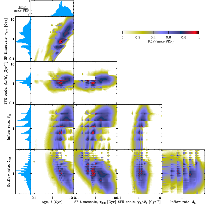
Figure 17: Posterior distribution of the SFH-related parameters. The plotting conventions are identical to Fig. 16. The displayed PDF is the distribution of the individual parameters of every galaxy, marginalizing over the dust evolution tuning parameters.

5.3.2 The Dust Evolution Timescales

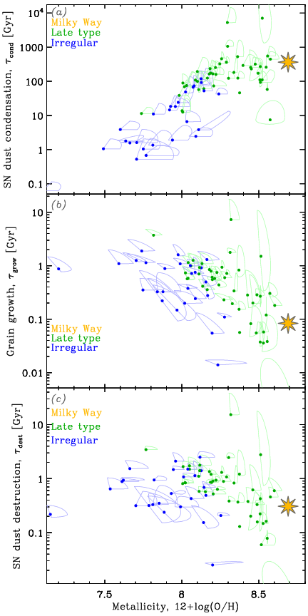
Figure 18: Dust evolution timescales, assuming a Salpeter (1955) IMF. The three panels display the posterior PDF of the three dust evolution timescales. The SUEs represent the value of these timescales as a function of metallicity, for each galaxy. The yellow star represents the Milky Way, at the maximum a posteriori of the three tuning parameters.

It is possible to estimate the posterior PDF of the dust evolution timescales of each galaxy, from the inferred parameters of Figs. 16 – 17, using Eqs. (11) – (14). Fig. 18 displays these timescales as a function of metallicity. Although there is some scatter due to the different SFH and age of galaxies in a given metallicity bin, we note that these timescales evolve.

The SN II dust condensation timescale

(panel (a) of Fig. 18) is around $\tau_{\mbox{{\scriptsize cond}}}\simeq 100$ Myr for ELMGs, implying that dust can be dominated by stardust in this regime. It rises up to $\tau_{\mbox{{\scriptsize cond}}}\simeq 1000$ Gyr around solar metallicity, indicating this process is not sufficient to account for all ISM dust in evolved systems.

The grain growth timescale

(panel (b) of Fig. 18) is quite scattered. It starts around $\tau_{\mbox{{\scriptsize grow}}}\simeq 1$ Gyr in the ELMG regime and decreases down to $\tau_{\mbox{{\scriptsize grow}}}\simeq 50$ Myr around solar metallicity. The average value of our sample at $12+\log(\textnormal{O/H})\geq 8.5$ is $\tau_{\mbox{{\scriptsize grow}}}\simeq 45$ Myr. It is another way to show that dust formation is dominated by grain growth around solar metallicity.

The SN II dust destruction timescale

(panel (c) of Fig. 18) is also scattered but stays around $\tau_{\mbox{{\scriptsize dest}}}\simeq 300$ Myr across our metallicity range.

The Milky Way value displayed in the three panels is consistent with the cloud of points in the highest metallicity domain.

There is a common misconception that dust destruction by SN II blast waves is unimportant at early-stages, because the dustiness is so low that few grains are destroyed by a single SN II. However, we show here that this is not the case as: 1 the SN II rate is on average higher at low-metallicity; 2 the fraction of grains destroyed by a single SN II is dustiness-independent.

5.3.3 Sensitivity to the IMF

As we discussed in Sects. 2.2.3 – 2.2.4, the main uncertainty on our estimated $M_{\star}$ and SFR comes from our IMF assumptions. Those were derived with a Salpeter (1955) IMF. Here, we explore the sensitivity of our results assuming a Chabrier (2003) IMF. To be consistent, we first need to correct our estimated $M_{\star}$ and SFR. According to Madau & Dickinson (2014, Sect. 3.1), we need to multiply SFR by 0.63 and $M_{\star}$ by 0.61. We have then generated another grid of models similar to Table 6 with the Chabrier (2003) IMF, and performed the fitting process of Sect. 5.2.3. The full results are given in Appendix G. The upshot is that the inferred tuning parameters are roughly consistent with our estimates in Sect. 5.3.1:

• $\langle Y_{\mbox{{\scriptsize SN}}}\rangle\simeq 2.5_{-0.3}^{+0.2}\times 10^{-2}\;\textnormal{M}_{\odot}/\textnormal{SN}$;

• $\epsilon_{\mbox{{\scriptsize grow}}}\simeq 4485_{-17}^{+11}$;

• $m_{\mbox{{\scriptsize gas}}}^{\mbox{{\scriptsize dest}}}\simeq 1289_{-7}^{+6}\;\textnormal{M}_{\odot}/\textnormal{SN}$.

The differences can be explained by the different relative contribution from LIMSs. The only value that differs sensibly is $\langle Y_{\mbox{{\scriptsize SN}}}\rangle$. This difference is however simply due to the fact the low-metallicity dustiness is overshot by the model with the Chabrier (2003) IMF.

This agreement was expected. The reason is that, to first order, LIMSs represent a dead weight in both the SED and the chemical enrichment. The total power emitted by stellar populations is dominated by massive stars. This is the reason why SFR and $M_{\star}$ estimates are so dependent on the IMF assumption. From the dust evolution modelling, the elemental and stardust enrichment is also dominated by massive stars. The only quantity for which we infer a different value is logically $\psi_{0}$. It is $\simeq 50\,\%$ higher to generate the same number of massive stars, compensating for the 0.63 correction factor.

5.4 Discussion

5.4.1 On the Low Inferred SN II Dust Yield

Our SN II dust yield is lower than the most recent estimates in situ. Measuring the dust mass produced by a single SN II is quite difficult, as it implies disentangling the freshly-formed dust from the surrounding ISM. It also carries the usual uncertainty about dust optical properties. A decade ago, the largest dust yield ever measured was $Y_{\mbox{{\scriptsize SN}}}\simeq 0.02\;\textnormal{M}_{\odot}$ (in SN 2003gd; Sugerman et al., 2006). The Herschel space telescope has been instrumental in estimating the cold mass of SuperNova Remnants (SNR). The yields of the three most well-studied SNRs are now an order of magnitude higher:

Cassiopeia A:

$Y_{\mbox{{\scriptsize SN}}}\simeq 0.04-1.1\;\textnormal{M}_{\odot}$ (Barlow et al., 2010; Arendt et al., 2014; De Looze et al., 2017; Bevan et al., 2017; Priestley et al., 2019);

The Crab nebula:

$Y_{\mbox{{\scriptsize SN}}}\simeq 0.03-0.23\;\textnormal{M}_{\odot}$ (Gomez et al., 2012; Temim & Dwek, 2013; De Looze et al., 2019);

SN 1987A:

$Y_{\mbox{{\scriptsize SN}}}\simeq 0.45-0.8\;\textnormal{M}_{\odot}$ (Dwek & Arendt, 2015; Matsuura et al., 2015).

In all these cases, the newly-formed grains have not yet experienced the reverse shock (Bocchio et al., 2016). The net yield is thus expected to be significantly lower.

Even if $\simeq 10-20\,\%$ of the dust condensed in an SN II ejecta survives its reverse shock (e.g.  Nozawa et al., 2006; Micelotta et al., 2016; Bocchio et al., 2016), we have to also consider the fact that massive stars are born in clusters. The freshly-formed dust injected by a particular SN II, having survived the reverse shock, will thus be exposed to the forward shock waves of nearby SNe II (e.g.  Martínez-González et al., 2018). This effect is not accounted for by Eq. (14), as it does not account for clustering, nor does it account for the excess dustiness around these stars due to the recent grain production. Our estimate of $\langle Y_{\mbox{{\scriptsize SN}}}\rangle$ is therefore an effective empirical yield, that probably accounts for this effect.

5.4.2 The Relevance of Local Low-Metallicity Galaxies

Our analysis confirms the long-lasting consensus that Milky Way dust is essentially grown in the ISM (Sect. 1). The apparently paradoxical fact here is that we have drawn this conclusion from the low-metallicity domain. It is because dust production is dominated by SN II condensation below the critical metallicity that we could constrain its efficiency and show it is unimportant at solar metallicity. The relevance of dwarf galaxies here is not necessarily that they can be considered as analogs of primordial distant galaxies, but that they sample a particular, key, dust production regime.

5.4.3 Implications for High-Redshift Systems

High-redshift ($z\gtrsim 6$) objects exhibiting copious amounts of dust ($\simeq 10^{7}-10^{8}\;\textnormal{M}_{\odot}$), close to the reionization era, have been challenging grain formation scenarios (e.g.  Dwek et al., 2007; Valiante et al., 2009; Dwek et al., 2014; Laporte et al., 2017). These objects are indeed only a few 100 Myr old, but have a roughly Galactic dustiness. SN II dust condensation would need to have a high efficiency ($\simeq 1\;\textnormal{M}_{\odot}/\textnormal{SN}$) to account for the observed dust mass (Dwek et al., 2007, 2014). AGB star yield can explain this dust content for $z\simeq 6$ objects (Valiante et al., 2009), but not at $z\simeq 8$ (Laporte et al., 2017).

Our results imply that grain growth should be the dominant dust formation mechanism in these galaxies. The dustiness of these massive objects being roughly Galactic, their metallicity should thus be Galactic too. The grain growth timescale should therefore be shorter than $\simeq 100$ Myr (panel (b) of Fig. 18), well below the age of these systems. Consequently, these very distant galaxies may not be the best laboratories to constrain the SN II dust yield.

5.4.4 Comparison with Recent Studies

As stated in Sects. 1 and 5.2.3, past studies have not been rigorously fitting cosmic dust evolution models to observations of galaxies. Recently, N20 and De Looze et al. (2020, hereafter DL20) have addressed this issue. N20 have adopted a relatively coarse dust evolution model grid with a frequentist fitting approach. Although interesting, their approach does not allow them to rigorously quantify parameter degeneracies and uncertainties. The comparison with their results is therefore limited. We have discussed the main discrepancies between the present work and theirs in Sects. 2.1.2 and Sect. 5.2.3.

DL20 have analyzed the JINGLE galaxy sample, following a methodology similar to ours, fitting the IR SED of each galaxy, and subsequently fitting one-zone dust evolution tracks to their derived $M_{\star}$, $M_{\mbox{{\scriptsize gas}}}$, $M_{\mbox{{\scriptsize dust}}}$, $Z$ and SFR. They adopted a non-hierarchical Bayesian approach. To our knowledge, this is the first article, similar to ours, to perform a rigorous fit of dust evolution models, with clearly quantified parameter uncertainties. Their results however qualitatively differ from ours. DL20 find an overall high SN II dust yield, and a low grain growth efficiency (the tuning parameters are not assumed universal in their study). In our opinion, the discrepancy between our results and those of DL20 comes from the two following points.

1. DL20’s metallicity coverage is more limited than ours. They have only one source below $12+\log(\textnormal{O/H})=8.0$, and none below $12+\log(\textnormal{O/H})=7.8$ (see e.g. their figure 7). Consequently, they do not sample the stardust regime, below the critical metallicity. Disentangling SN II dust condensation, grain growth and shock destruction, with their data, is therefore rendered difficult.

2. The posterior distribution of the dust evolution parameters inferred by DL20, as seen in their figures G.7 to G.12 (they focus their analysis on their galaxy bins 3 and 4), rarely goes down to zero probability within the range allowed by their uniform prior. It means the weight of evidence provided by their data is relatively mild. Our inference of $\epsilon_{\mbox{{\scriptsize grow}}}$ and $m_{\mbox{{\scriptsize gas}}}^{\mbox{{\scriptsize dest}}}$ are consistent with their PDF, as they fall in a high probability domain in all their models. We simply have a smaller uncertainty, thanks to our low-metallicity coverage. This is more pronounced for their distribution of $\delta_{\mbox{{\scriptsize SN}}}$ (their $f_{\mbox{{\scriptsize survival}}}$). DL20 would have also benefitted from extending their prior range down to smaller values, as they do not consider yields below $\delta_{\mbox{{\scriptsize SN}}}=10\,\%$, while we infer a value around $\delta_{\mbox{{\scriptsize SN}}}\simeq 1\,\%$.

6 SUMMARY AND CONCLUSION

This article has presented an observational study aimed at constraining the timescales of the main processes controlling the evolution of interstellar dust in galaxies. The principal highlights are the following.

1. We have gathered the 3-$\mu\textnormal{m}$-to-1-mm photometry and ancillary data of 798 nearby galaxies from the DustPedia (Davies et al., 2017) and DGS (Madden et al., 2013) surveys. We have attempted to create the most conservative, homogeneous sample, by controlling the factors that could lead to systematic biases (Sect. 2):

   1. the DustPedia and DGS IR data reduction and photometry have been performed consistently;

   2. the stellar mass and SFR have been estimated using the same IMF;

   3. the metallicities have been estimated using one uniform calibration;

   4. the total gas masses have been derived from [H i]${}_{21\,\textnormal{cm}}$ and ¹²CO(J$=$1$\rightarrow$0)${}_{2.6\textnormal{mm}}$ observations, when available. When CO data was not available, the molecular gas mass was estimated from a scaling relation.

   5. Resolved interferometric [H i]${}_{21\,\textnormal{cm}}$ observations of 20 of the lowest metallicity objects were used in order to extract the gas mass corresponding exactly to the IR photometric aperture.

2. We have performed a hierarchical Bayesian dust SED fit of the 798 galaxies, using the code HerBIE (G18) with the THEMIS grain properties (Jones et al., 2017).

   1. This allowed us to infer the dust mass, $M_{\mbox{{\scriptsize dust}}}$, mean starlight intensity, $\langle U\rangle$, and the mass fraction of aromatic-feature-emitting grains, $q_{\mbox{{\scriptsize AF}}}$, in each galaxy (Sect. 3.2). The inferred parameters are given in Table H.

   2. We have compared our inferred parameters to a series of additional runs, as well as to independent literature studies, in order to demonstrate the influence of the different assumptions of our model and assess the robustness of our results (Sects. 3.3 – 3.4).

3. We have displayed several well-known scaling relations involving $M_{\star}$, $M_{\mbox{{\scriptsize gas}}}$, $M_{\mbox{{\scriptsize dust}}}$, $12+\log(\textnormal{O/H})$, SFR, $q_{\mbox{{\scriptsize AF}}}$ and $\langle U\rangle$, for our sample (Sect. 4).

   1. We have shown that there is a drastic evolution with metallicity of the dust-to-metal mass ratio (by two orders of magnitude). We have extensively discussed the different biases that could artificially produce such a trend, concluding they were unlikely (Sect. 4.1.3).

   2. We have noticed that early-type galaxies have a systematically lower dust-to-gas mass ratio than other types in the same gas-to-stellar mass ratio range. We have investigated the possibility that this was resulting from the enhanced dust destruction due to thermal sputtering in the hot X-ray emitting gas permeating these objects. This scenario is supported by a rough negative correlation between the dust-to-star mass ratio and the X-ray photon rate per dust grain (Sect. 4.1.2).

   3. We have displayed the well-known trends of $q_{\mbox{{\scriptsize AF}}}$ with $12+\log(\textnormal{O/H})$ and $\langle U\rangle$. Our data indicate the correlation with $12+\log(\textnormal{O/H})$ is significantly better (Sect. 4.2). It implies that, at the scale of a galaxy, the overall abundance of small a-C(:H) grains might be principally controlled by the efficiency of their formation (stardust production and/or shattering of larger carbon grains). The photodestruction of small a-C(:H) might overall be circumscribed around star forming regions.

4. We have performed a hierarchical Bayesian fit of a one-zone dust evolution model to the derived $M_{\star}$, $M_{\mbox{{\scriptsize gas}}}$, $M_{\mbox{{\scriptsize dust}}}$, $12+\log(\textnormal{O/H})$ and SFR of a subsample of 556 late-type and irregular objects (Sect. 5).

   1. We have inferred the efficiency of the three main dust evolution tuning parameters (Sect. 5.3): 1 the IMF-averaged SN II dust yield is $\langle Y_{\mbox{{\scriptsize SN}}}\rangle\lesssim 0.03\;\textnormal{M}_{\odot}/\textnormal{SN}$; 2 the grain growth efficiency parameter (Mattsson et al., 2012) is $\epsilon_{\mbox{{\scriptsize grow}}}\gtrsim 3000$; 3 the average gas mass cleared of dust by a single SN II shock wave is $m_{\mbox{{\scriptsize gas}}}^{\mbox{{\scriptsize dest}}}\gtrsim 1200\;\textnormal{M}_{\odot}/\textnormal{SN}$. Our results therefore imply that dust production is dominated by grain growth in the ISM above a critical metallicity of $12+\log(\textnormal{O/H})\simeq 8.0$. They also suggest that the massive amounts of dust detected in high redshift systems ($z\gtrsim 6$) likely grew in the ISM.

   2. We have shown that ELMGs were crucial in constraining these parameters, as they sample a regime where dust production is dominated by SN II condensation. A steep, strongly non-linear, dustiness-metallicity relation, such as the one we have found, is the unambiguous evidence that stardust can not dominate the content of solar metallicity systems.

   3. We have shown and explained why these conclusions were, to first order, independent of our IMF assumption (Sect. 5.3.3).

   4. Our model fails at reproducing the relation between the sSFR and the dust-to-star mass ratio. We suspect this is due to the oversimplicity of our SFH, inflow and outflow prescriptions.

Several of the limitations of our study could be addressed by spatially resolving star forming regions. Performing a similar analysis on $\simeq 100$ pc scales within galaxies would allow us to access another important parameter: the density of the ISM. This quantity drives mantle growth and coagulation. Local variations of the dust-to-metal mass ratio are good indications of grain growth and can help us break the degeneracy with SN II destruction (Sect. 5.2.2). In addition, spatial resolution would be a way to address the origin of the trend of $q_{\mbox{{\scriptsize AF}}}$ with metallicity (Sect. 4.2), as well as resolving ETGs to quantify the grain sputtering timescale (Sect. 4.1.2). Numerous spatially resolved dust studies have already been published (e.g.  Galliano et al., 2011; Mattsson & Andersen, 2012; Draine & Hensley, 2013; Hunt et al., 2015; Roman-Duval et al., 2017; Aniano et al., 2020). We are currently preparing several papers of a resolved subsample, with the same consistent approach as employed in the present manuscript (Roychowdhury et al.; Casasola et al., in prep.). The main observational challenge in order to address these degeneracies is however to obtain spatial resolution in ELMGs, at far-IR wavelengths. The data are currently very limited, because the sensitivity of Herschel was not high enough. SPICA (van der Tak et al., 2018) was the only observatory on the horizon to have the sensitivity to produce resolved far-IR maps of ELMGs. Its sudden cancellation by ESA might leave the important open questions raised in this paper unanswered for several decades.

Appendix A CALIBRATION UNCERTAINTIES

The HB approach is one of the only methods allowing a rigorous treatment of the photometric calibration uncertainties. These uncertainties are indeed systematic effects, with both spectral and spatial correlations. Some studies account for their spectral correlations, but ignore their spatial correlations (e.g.  Gordon et al., 2014). In the present paper, following G18, we assume that calibration uncertainties are perfectly correlated between sources, and partially correlated between wavelengths. In this section, we discuss the values of these uncertainties and of their correlation coefficients.

The DustPedia photometric fluxes, given in the archive, $F_{\nu}(\lambda_{0})$ at wavelength $\lambda_{0}$, are accompanied with a total uncertainty being the quadratic sum of noise and calibration errors:

$$\sigma_{\nu}^{\mbox{{\scriptsize C18}}}(\lambda_{0})=\sqrt{\left(\sigma_{\nu}^{\mbox{{\scriptsize noise}}}(\lambda_{0})\right)^{2}+\left(\delta_{\mbox{{\scriptsize cal}}}^{\mbox{{\scriptsize C18}}}(\lambda_{0})\times F_{\nu}(\lambda_{0})\right)^{2}},$$ (17)

where $\delta_{\mbox{{\scriptsize cal}}}^{\mbox{{\scriptsize C18}}}(\lambda_{0})$ is the calibration uncertainty (Table 1 of C18, ). HerBIE treats the noise and calibration uncertainties separately. Therefore, we keep the noise uncertainty, $\sigma_{\nu}^{\mbox{{\scriptsize noise}}}(\lambda_{0})$, but we build a covariance matrix of the absolute calibration uncertainties, $V_{\mbox{{\scriptsize cal}}}$, to replace the $\delta_{\mbox{{\scriptsize cal}}}^{\mbox{{\scriptsize C18}}}$ coefficients.

A.1 The Full Covariance Matrix

Using the separation strategy (Barnard et al., 2000), we decompose the covariance matrix of the absolute calibration uncertainties as:

$$V_{\mbox{{\scriptsize cal}}}=S_{\mbox{{\scriptsize cal}}}R_{\mbox{{\scriptsize cal}}}S_{\mbox{{\scriptsize cal}}},$$ (18)

where $S_{\mbox{{\scriptsize cal}}}$ is the diagonal matrix of standard-deviations and $R_{\mbox{{\scriptsize cal}}}$ the correlation matrix. The non-trivial elements of $S_{\mbox{{\scriptsize cal}}}$ and $R_{\mbox{{\scriptsize cal}}}$ are given in Tables 7 – 8. We describe, in the following sections A.2 to A.8, how we obtained these values from the literature.

Table 7: Absolute calibration uncertainties (diagonal of $S_{\mbox{{\scriptsize cal}}}$; Eq. 18). See Table 1 for waveband naming conventions.

Waveband label	Calibration uncertainty
IRAC1	$10.2\,\%$
IRAC2	$10.2\,\%$
IRAC3	$10.2\,\%$
IRAC4	$10.2\,\%$
MIPS1	$4.0\,\%$
MIPS2	$5.0\,\%$
MIPS3	$11.6\,\%$
PACS1	$5.4\,\%$
PACS2	$5.4\,\%$
PACS3	$5.4\,\%$
SPIRE1	$5.9\,\%$
SPIRE2	$5.9\,\%$
SPIRE3	$5.9\,\%$
WISE1	$3.2\,\%$
WISE2	$3.5\,\%$
WISE3	$5.0\,\%$
WISE4	$7.0\,\%$
IRAS1	$7.6\,\%$
IRAS2	$11.0\,\%$
IRAS3	$14.6\,\%$
IRAS4	$20.2\,\%$
HFI1	$4.3\,\%$
HFI2	$4.2\,\%$
HFI3	$0.90\,\%$

Table 8: Correlations of the absolute calibration uncertainties ($R_{\mbox{{\scriptsize cal}}}$ matrix; Eq. 18). See Table 1 for waveband naming conventions.

	IRAC				MIPS			PACS			SPIRE			WISE				IRAS				HFI
IRAC1	1	0.02	0.02	0.02	0	0	0	0	0	0	0	0	0	0.13	0.06	0.04	0	0	0	0	0	0	0	0
IRAC2	0.02	1	0.02	0.02	0	0	0	0	0	0	0	0	0	0.07	0.12	0.04	0	0	0	0	0	0	0	0
IRAC3	0.02	0.02	1	0.02	0	0	0	0	0	0	0	0	0	0.07	0.06	0.04	0	0	0	0	0	0	0	0
IRAC4	0.02	0.02	0.02	1	0	0	0	0	0	0	0	0	0	0.07	0.06	0.09	0	0	0	0	0	0	0	0
MIPS1	0	0	0	0	1	0	0.34	0	0	0	0	0	0	0	0	0	0.57	0	0	0	0	0	0	0
MIPS2	0	0	0	0	0	1	0.43	0	0	0	0	0	0	0	0	0	0	0	0	0	0	0	0	0
MIPS3	0	0	0	0	0.34	0.43	1	0	0	0	0	0	0	0	0	0	0.20	0	0	0	0	0	0	0
PACS1	0	0	0	0	0	0	0	1	0.86	0.86	0	0	0	0	0	0	0	0	0	0	0	0	0	0
PACS2	0	0	0	0	0	0	0	0.86	1	0.86	0	0	0	0	0	0	0	0	0	0	0	0	0	0
PACS3	0	0	0	0	0	0	0	0.86	0.86	1	0	0	0	0	0	0	0	0	0	0	0	0	0	0
SPIRE1	0	0	0	0	0	0	0	0	0	0	1	0.47	0.47	0	0	0	0	0	0	0	0	0.40	0.41	0
SPIRE2	0	0	0	0	0	0	0	0	0	0	0.47	1	0.47	0	0	0	0	0	0	0	0	0.40	0.41	0
SPIRE3	0	0	0	0	0	0	0	0	0	0	0.47	0.47	1	0	0	0	0	0	0	0	0	0.40	0.41	0
WISE1	0.13	0.07	0.07	0.07	0	0	0	0	0	0	0	0	0	1	0.21	0.14	0	0	0	0	0	0	0	0
WISE2	0.06	0.12	0.06	0.06	0	0	0	0	0	0	0	0	0	0.21	1	0.13	0	0	0	0	0	0	0	0
WISE3	0.04	0.04	0.04	0.09	0	0	0	0	0	0	0	0	0	0.14	0.13	1	0	0	0	0	0	0	0	0
WISE4	0	0	0	0	0.57	0	0.20	0	0	0	0	0	0	0	0	0	1	0	0	0	0	0	0	0
IRAS1	0	0	0	0	0	0	0	0	0	0	0	0	0	0	0	0	0	1	0.69	0.52	0.38	0	0	0
IRAS2	0	0	0	0	0	0	0	0	0	0	0	0	0	0	0	0	0	0.69	1	0.36	0.26	0	0	0
IRAS3	0	0	0	0	0	0	0	0	0	0	0	0	0	0	0	0	0	0.52	0.36	1	0.72	0	0	0
IRAS4	0	0	0	0	0	0	0	0	0	0	0	0	0	0	0	0	0	0.38	0.26	0.72	1	0	0	0
HFI1	0	0	0	0	0	0	0	0	0	0	0.40	0.40	0.40	0	0	0	0	0	0	0	0	1	0.69	0
HFI2	0	0	0	0	0	0	0	0	0	0	0.41	0.41	0.41	0	0	0	0	0	0	0	0	0.69	1	0
HFI3	0	0	0	0	0	0	0	0	0	0	0	0	0	0	0	0	0	0	0	0	0	0	0	1

A.2 Spitzer/IRAC

The calibration of IRAC data is presented by Reach et al. (2005). It is performed using a subsample of the stellar catalog of Cohen et al. (2003). The components entering in the uncertainty on the absolute calibration are given by Eq. (13) of Reach et al. (2005) and the corresponding values in their Table 7. The first term is the correlated uncertainty, $\sigma_{\mbox{{\scriptsize abs}}}=1.5\,\%$, corresponding to the uncertainty in the predicted fluxes of Vega and Sirius. The second term is the uncorrelated uncertainty on the calibrator fluxes: $\sqrt{(\sigma_{\mbox{{\scriptsize groud}}}^{2}-\sigma_{\mbox{{\scriptsize abs}}}^{2})/n}=0.87\,\%$, with $\sigma_{\mbox{{\scriptsize ground}}}=2.3\,\%$ and $n=4$. Finally, there is an uncorrelated term introduced by the dispersion of the IRAC observations of the calibrators: $\sigma_{\mbox{{\scriptsize rms}}}/\sqrt{n}$, where $\sigma_{\mbox{{\scriptsize rms}}}=2.0\,\%$, $1.9\,\%$, $2.1\,\%$ and $2.1\,\%$ for IRAC1, IRAC2, IRAC3 and IRAC4, respectively.

In addition, one must multiply the point source calibrated fluxes by aperture correction factors. According to the IRAC instrument handbook (Sect. 4.11), these factors have a $10\,\%$ uncertainty. We include this extra source of uncertainty, assuming it is uncorrelated. These correction factors have been applied by C18 for all the DustPedia galaxies and by Rémy-Ruyer et al. (2015) for half of the DGS galaxies, the other half being nearly point sources. The IRAC calibration uncertainties will thus be overestimated for about 15 of our sources.

A.3 Spitzer/MIPS

MIPS calibration has been independently performed for each of its three wavebands. The 24 $\mu\textnormal{m}$ calibration is presented by Engelbracht et al. (2007). It is primarily based on observations of A stars. The authors recommend adopting a net calibration uncertainty of $4\,\%$. The 70 $\mu\textnormal{m}$ calibration is presented by Gordon et al. (2007). It is primarily based on observations of B and M stars. The authors recommend using a calibration uncertainty of $5\,\%$, dominated by repeatability scatter. Finally, the 160 $\mu\textnormal{m}$ calibration, presented by Stansberry et al. (2007) is performed on observations of asteroids, simulatenously in the three MIPS bands. This 160 $\mu\textnormal{m}$ calibration uncertainty is therefore tied to 24 and 70 $\mu\textnormal{m}$. The authors estimate a $7\,\%$ uncertainty tied to these bands, for a total uncertainty of $11.6\,\%$. To simplify, we assume that the calibration uncertainty is the quadratical sum of $4\,\%$ correlated with MIPS1, $5\,\%$ correlated with MIPS2, and the remaining $9.7\,\%$ uncorrelated.

A.4 Herschel/PACS

PACS calibration is performed on five stars, used as primary calibrators (Balog et al., 2014). The absolute calibration uncertainty for point sources appears to be dominated by the stellar model uncertainty of $5\,\%$, correlated between bands. In addition, there is a $2\,\%$ repeatability uncertainty, uncorrelated between bands. The extended source calibration uncertainty is not quantified by the instrument team.

A.5 Herschel/SPIRE

SPIRE calibration, presented by Griffin et al. (2013) is performed on Neptune. The uncertainty comes from three sources. There is a $4\,\%$ correlated uncertainty on Neptune’s model. There is also a $1.5\,\%$ uncorrelated uncertainty due to the noise in Neptune’s observations. Finally, there is a $4\,\%$ uncorrelated uncertainty on SPIRE’s beam area.

A.6 WISE

WISE data have been calibrated by Jarrett et al. (2011) using observations of a network of stars in both ecliptic poles (Cohen et al., 2003) and an additional red source, the galaxy NGC 6552. These calibrators have been observed with Spitzer/IRAC and Spitzer/MIPS, and compared to WISE. It appears that the relative WISE calibration, tied to Spitzer, is accurate to $2.4\,\%$, $2.8\,\%$, $4.5\,\%$ and $5.7\,\%$ (for WISE1, WISE2, WISE3 and WISE4, respectively). These uncertainties come from the scatter of individual calibrators and can therefore be considered independent. The red calibrator (NGC 6552) is reported to be too bright by $\simeq 6\,\%$ by Jarrett et al. (2011). However, Brown et al. (2014) revised the central wavelength of the WISE4 band to correct systematic discrepancies observed with red sources.

The absolute calibration accuracy of WISE is not discussed by Jarrett et al. (2011). We can simply assume that each WISE band will be tied to the closest Spitzer band: WISE1 with IRAC1; WISE2 with IRAC2; WISE3 with IRAC4; WISE4 with MIPS1. We can thus quadratically add the Spitzer calibration uncertainties to these bands and assume that this term will be correlated with the Spitzer bands. However, we do not include the IRAC uncertainty on the extended source correction (Appendix A.2), as these calibrators are point sources.

A.7 IRAS

The IRAS flux calibration is presented by Wheelock et al. (1994, Sect. VI.C.2). The 12 $\mu\textnormal{m}$ flux is calibrated on observations of the star $\alpha$-Tau, assuming the absolute flux value derived from the ground-based 10 $\mu\textnormal{m}$ photometry by Rieke et al. (1985), accurate within $3\,\%$. An additional source of error comes from the uncertainty of $2\,\%$ on the model used to extrapolate the flux at 12 $\mu\textnormal{m}$. The 25 and 60 $\mu\textnormal{m}$ fluxes are calibrated by extrapolating the 12 $\mu\textnormal{m}$ flux, using stellar models, normalized to the Sun. The uncertainty in this extrapolation, based on the scatter of individual stars, is estimated to be $4\,\%$ and $5.3\,\%$, respectively (Table VI..C.1 of Wheelock et al., 1994). These uncertainties, which can be assumed to be independent, have to be quadratically added to the 12 $\mu\textnormal{m}$ uncertainty, which is a fully correlated term. The 100 $\mu\textnormal{m}$ calibration is based on observations of asteroids, where the 60 $\mu\textnormal{m}$ flux is extrapolated to 100 $\mu\textnormal{m}$, assuming that the 25/60 and 60/100 color temperatures are identical. Wheelock et al. (1994) estimate that the total relative calibration uncertainty at 100 $\mu\textnormal{m}$ is $10\,\%$, due to the model uncertainty and scatter of the asteroid observations. This uncertainty is correlated with the 60 $\mu\textnormal{m}$.

For extended sources, uncertainties in the frequency response and the effective detector area have to be considered (Wheelock et al., 1994, Sect. VI.C.4). The uncertainty on the frequency response is not fully quantified, except that it should be $7\,\%$/$\mu\textnormal{m}$ of the central bandwidth, with an uncertainty of 0.3 $\mu\textnormal{m}$ on the bandwidth (Sect. VI.C.3 of Wheelock et al., 1994). It is also specified that the 100 $\mu\textnormal{m}$ uncertainty can be significant for objects cooler than 30 K, which is our case. The uncertainty on the detector areas is given by Table IV.A.1 of Wheelock et al. (1994) showing the flux dispersion of each individual detector, during a cross-scan of the planetary nebula NGC 6543. The average dispersions of $6.4\,\%$, $6.5\,\%$, $11\,\%$ and $10.9\,\%$ (for IRAS1, IRAS2, IRAS3 and IRAS4, respectively) can be considered as an additional, independent source of uncertainty.

A.8 Planck/HFI

The calibration of the HFI data used by C18 is presented by Planck Collaboration et al. (2016). The two short wavelength bands (350 and 550 $\mu\textnormal{m}$) are calibrated on Neptune and Uranus. The uncertainty on the model is $5\,\%$ including $2\,\%$ spectrally independent. The statistical errors on the observations of the calibrators are $1.4\,\%$ and $1.1\,\%$, respectively, which can be considered independent. The models of Neptune used here and for SPIRE (Appendix A.5) are the ESA3 and ESA4 models (ftp://ftp.sciops.esa.int/pub/hsc-calibration/PlanetaryModels/), respectively. Both models differ only by 0.3–0.6$\,\%$ in the SPIRE and HFI bands. They will thus induce correlation. To simplify, we assume that the HFI calibration factors derived from Neptune (correlated with SPIRE) and Uranus (not correlated with SPIRE) are averaged. We obtain calibration uncertainties $\simeq 30\,\%$ lower than Planck Collaboration et al. (2016), as they have opted for the more conservative, linear addition of independent errors. We choose here the more rigorous quadratrical addition.

The four long wavelength bands of HFI are calibrated on the CMB dipole. The first source of uncertainty is the scatter of individual bolometers: $0.78\,\%$, $0.16\,\%$, $0.07\,\%$ and $0.09\,\%$ at 850 $\mu\textnormal{m}$, 1.38, 2.1 and 3.0 mm. The second source of uncertainty comes from the gain variations: $0.03\,\%$, $0.04\,\%$, $0.05\,\%$ and $0.05\,\%$, respectively. These different uncertainties can be considered independent.

Appendix B HOMOGENEITY OF THE SAMPLE

B.1 DustPedia and DGS Photometry

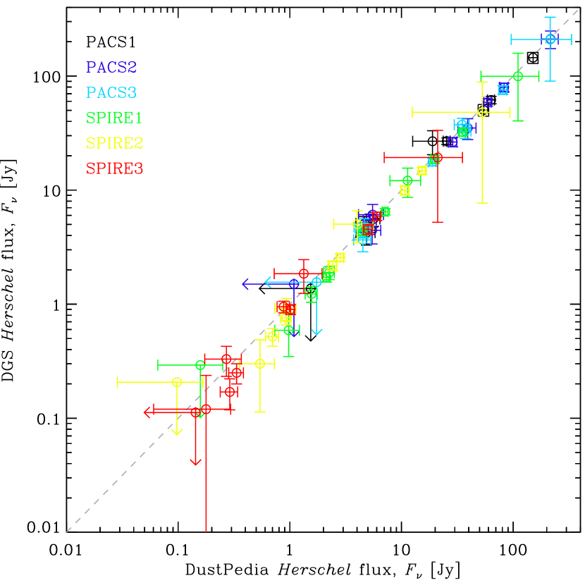
Figure 19: Comparison between the DustPedia and DGS photometry. The 13 sources of the DGS which are part of the DustPedia catalog are compared in the 3 PACS and 3 SPIRE bands (one color per filter). The $x$ axis shows the photometry estimated by C18, while the $y$ axis shows the photometry estimated by Rémy-Ruyer et al. (2015). The dashed line represents the 1:1 relation.

Fig. 19 displays the comparison, in the 6 Herschel bands, of the photometry of the sources of the DGS that are part of the DustPedia sample. The DustPedia photometry has been estimated by C18 (cf. Sect. 2.1.1), and the DGS photometry, by Rémy-Ruyer et al. (2015, cf. Sect. 2.1.2). Both are in very good agreement.

B.2 Derivation of the Stellar Mass

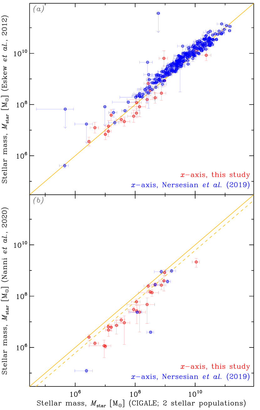
Figure 20: Comparison of stellar mass estimators. Panel (a) compares the CIGALE estimates of $M_{\star}$, using two stellar populations ($x$-axis), with the Eskew et al. (2012, $y$-axis) empirical approximation, both assuming a Salpeter (1955) IMF. Panel (b) compares the same $x$-axis as panel (a) to the CIGALE estimates, using a single stellar population and a Chabrier (2003) IMF, by N20. In both panels, the blue symbols correspond to the values presented in Nersesian et al. (2019), and the red symbols correspond to the values estimated for this study, with the same CIGALE settings. The solid yellow line represents the 1:1 relation. The dashed yellow line in panel (b) represents the 1:0.61 relation that accounts for the difference in IMFs.

To further investigate the discrepancy between the CIGALE fits of N20 and the Eskew et al. (2012) approximation used by Madden et al. (2014), discussed in Sect. 2.2.1, we have compared the two estimators on our sample. To close the controversy, we have modelled the UV-to-mm SED of the 35 DGS galaxies that were not in DustPedia, with CIGALE, using the same settings as Nersesian et al. (2019, i.e. using two stellar populations). We therefore have CIGALE-derived $M_{\star}$ for our whole sample. This is shown in panel (a) of Fig. 20. The stellar mass derived using CIGALE with two stellar populations are in very good agreement with the Eskew et al. (2012) approximation.

Panel (b) of Fig. 20 compares the same CIGALE-two-population estimates with the values of $M_{\star}$ reported by N20. The main differences are the following, noting that the stellar masses quoted by N20 come from the SED modelling presented by Burgarella et al. (2020).

1. Nersesian et al. (2019) used the UV-optical photometry of Clark et al. (2018), which have been homogenized (cf. Sect. 2.1), whereas Burgarella et al. (2020) gathered UV-optical data from the NASA/IPAC Extragalactic Database (NED). The latter is a compilation of data from the literature that can be inhomogeneous in terms of photometric aperture, extinction correction and removal of foreground stars.

2. Nersesian et al. (2019) used CIGALE with two stellar populations: 1 an old exponentially decreasing SFH; 2 a young burst. In contrast, Burgarella et al. (2020) used a single delayed SFH, which can lead to underestimating the mass, because of the outshining effect of the recent star formation (e.g.  Lopes et al., 2020). For instance, Buat et al. (2014) conducted a large comparison of stellar mass estimates and concluded that models using two stellar populations were providing the best fits. This can explain why the IRAC1 and IRAC2 fluxes are systematically underestimated by the mean model of N20 (cf. their figure A.1), while it is not the case for Nersesian et al. (2019, http://dustpedia.astro.noa.gr/Cigale). Yet, these bands sample the spectral range where the bulk of the stellar mass dominates the emission. In addition, most of the galaxies of the DGS are Blue Compact Dwarf galaxies (BCD). These galaxies are known to be actively forming stars and have an old underlying stellar population (e.g.  Hunter & Gallagher, 1989; Grebel, 1999; Kunth & Östlin, 2000; Aloisi et al., 2007; Janowiecki et al., 2017).

3. Nersesian et al. (2019) used a Salpeter (1955) IMF, whereas Burgarella et al. (2020) used a Chabrier (2003) IMF leading to a systematic scaling by a factor 0.61.

The comparison of these two estimates, in panel (b) of Fig. 20, shows that the stellar masses of N20 are most of the time systematically lower than those of Nersesian et al. (2019), sometimes drastically.

Appendix C ADDITIONAL DISCUSSION ON THE PARAMETRIZATION OF THEMIS

We have presented the way we parametrize the THEMIS size distribution in Sect. 3.1.1. It consists in linearly scaling the fractions of a-C(:H) smaller than 7 Å, and between 7 and 15 Å. We call it the linear parametrization. It is controlled by the two parameters $q_{\mbox{{\scriptsize AF}}}$ and $f_{\mbox{{\scriptsize VSAC}}}$, introduced in Sect. 3.1.1. In the present appendix, we demonstrate, on an example, that this parametrization is flexible enough to mimic the original parametrization of THEMIS. The THEMIS size distribution of small a-C(:H) is a power-law, with minimum cut-off size $a_{\mbox{{\scriptsize min}}}=4\;\AA$ and index $\alpha=5$ (Table 2 of Jones et al., 2013). We call it the non-linear parametrization. Varying $a_{\mbox{{\scriptsize min}}}$ and $\alpha$ is probably more physical than our linear method, as it preserves the continuity of the size distribution. However, it produces SEDs with very similar shapes.

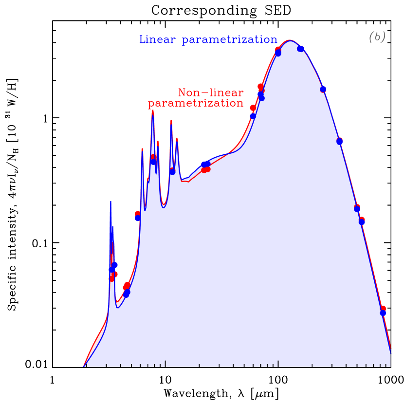
Figure 21: THEMIS parametrization comparison. The two panels display the same quantities as Fig. 1. On each panel, the red curve shows THEMIS, non-linearly parametrized, i.e. varying the minimum cut-off radius, $a_{\mbox{{\scriptsize min}}}$, and the index of the power-law1 size distribution, $\alpha$. The blue curve shows THEMIS, linearly parametrized, with the method described in Sect. 3.1.1. The dots on the two SED curves (panel b) represent the synthetic photometry, i.e. the model integrated in the filters of Table 1.

This is demonstrated on Fig. 21. This figure displays the same quantities as Fig. 1, but compares the two parametrizations. The red curves show the size distribution (panel a) and the corresponding SED (panel b), for the non-linear method, with $a_{\mbox{{\scriptsize min}}}=5\;\AA$ and $\alpha=4$. The blue curves show the same quantities, with the linear method. We see that the broadband fluxes (dots in panel b) produced by these two parametrizations are very similar. The fact that they are not exactly the same is not important here. What is relevant is that the two methods can alter the SED with the same dynamical range.

Appendix D POSTERIOR PREDICTIVE P-VALUE

We have estimated the posterior predictive $p$-value (PPP; e.g. Gelman et al., 2004) of our reference run (Sect. 3.2). PPPs are the Bayesian equivalent to a chi-squared test. They allow us to quantify the goodness of our fit. PPPs are estimated by generating sets of replicated observables, noted $D_{\mbox{{\scriptsize rep}}}$, from our posterior distribution, conditional on the actual data (Sect. 2), noted $D$:

$$p(D_{\mbox{{\scriptsize rep}}}|D)=\int p(D_{\mbox{{\scriptsize rep}}}|X)p(X|D)\,\textnormal{d}X,$$ (19)

where $X$ are the model parameters. In practice, these replicated sets are simply estimated by computing the SED model for samples of the parameters drawn from the MCMC. The comparison to the data requires the assumption of a test statistic, $T(D,X)$. We adopt the commonly-used $\chi^{2}$ discrepancy quantity:

$$T(D,X)\equiv\sum_{i}\frac{\left[D_{i}-\mu(D_{i}|X)\right]^{2}}{\sigma(D_{i}|X)^{2}},$$ (20)

where the index $i$ represents every observable of every galaxy, and the quantities $\mu(D_{i}|X)$ and $\sigma(D_{i}|X)$ are the mean and standard-deviation of the replicated data. We then need to estimate the probability:

$$p_{B}\equiv P\left(T(D_{\mbox{{\scriptsize rep}}}|X)\geq T(D|X)\,|\,D\right).$$ (21)

If the difference between the replicated set and the data is solely due to statistical fluctuations, this probability should be on average $50\,\%$. A model passes the test, at the $98\,\%$ credence level, if $1\,\%<p_{B}<99\,\%$.

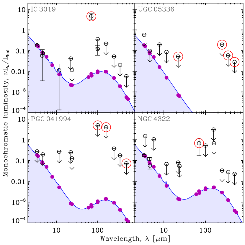
Figure 22: SEDs of the 4 galaxies causing the maximum deviations of the PPP. The black circles with error bars are the observables. Most of them are upper limits. The blue line is the maximum a posteriori model, and the purple dots are the synthetic photometry. The problematic fluxes are identified by a red circle.

In our case, we get $p_{B}=0.68\,\%$, indicating our model fails this test (it passes the $99\,\%$ credence level, though). Investigating the cause of this low $p$-value, we notice that a few observations are responsible for large deviations. Fig. 22 displays the SEDs containing the 9 most deviant fluxes.

IC 0319 and NGC 4322:

the problematic flux is PACS1. For IC 0319, it clearly lies above the rest of the observations, but has a small error bar. There is likely a problem with this particular measure. The problem is more difficult to assess for NGC 4322. However, the model is pulled well below this flux by the three SPIRE upper limits.

UGC 05336 and PGC 041994:

the problems come from several far-IR upper limits. We display $3\sigma$ upper limits when the value of the measured flux is smaller than its $1\sigma$ noise level. In the case of the highlighted bands, the actual value of the fluxes are negative, either because of statistical fluctuations, or background over-subtraction. Since the modelled flux can not be negative, we have $T(D_{\mbox{{\scriptsize rep}}}|X)\ll T(D|X)$ for all replicated sets, pulling $p_{B}$ to the tail of the distribution.

In summary, we are not in the case where the model would provide a poor fit on average. A few discrepant data, that are treated as outliers by the model (i.e. which have a very limited impact on the results), are responsible for failing the PPP test. Excluding these 9 observables, which represent only $0.07\,\%$ of our sample, we get $p_{B}=1.3\,\%$, making our model pass the test. In practice, such a test is quite strict, knowing the complexity of our hierarchical model and of the data. Indeed, the frequentist equivalent would be to test the chi-squared of all our SED fits at once. Accounting for missing data, the model for our 798 galaxies would have 3655 degrees of freedom. For a $98\,\%$ confidence level, the reduced chi-squared would be required to lie in the narrow range $0.95<\bar{\chi}^{2}<1.05$. This is because the more data we have, the smaller the statistical fluctuations should be.

Appendix E DERIVED TEMPERATURE-EMISSIVITY RELATION

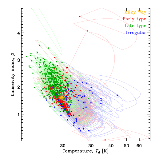
Figure 23: Modified black body results. The SUEs show the relation between the temperature, $T_{\mbox{{\scriptsize d}}}$, and the emissivity index, $\beta$, derived from the $\beta$-free MBB run presented in Sect. 3.3.2. Galaxies are color-coded according to their type (cf. Sect. 3.3.2). The diffuse ISM of the Milky Way ($T_{\mbox{{\scriptsize d}}}^{\mbox{{\scriptsize MW}}}=20$ K, $\beta_{\mbox{{\scriptsize MW}}}=1.6$; Planck Collaboration et al., 2014) is displayed as a yellow star.

Fig. 23 shows the $\beta-T_{\mbox{{\scriptsize d}}}$ relation derived from the HB MBB fit to the sample of Sect. 2 (cf. Sect. 3.3.2). We can see that most sources are clustered around $(T_{\mbox{{\scriptsize d}}};\beta)\simeq\left(18.7_{-0.2}^{+5.6}\,\textnormal{K};2.18_{-0.57}^{+0.00}\right)$, with $\pm 1\sigma$ distribution widths $\Delta T_{\mbox{{\scriptsize d}}}=\left[15.7_{--1.0}^{+0.8}\,\textnormal{K},22.2_{--1.0}^{+1.1}\,\textnormal{K}\right]$ and $\Delta\beta=\left[1.68_{-0.06}^{+0.02},2.68_{-0.06}^{+0.02}\right]$. The correlation coefficient is $\rho(\ln T_{\mbox{{\scriptsize d}}},\beta)\simeq-0.54_{-0.01}^{+0.18}$, and $\textnormal{CR}_{95\%}(\rho(\ln T_{\mbox{{\scriptsize d}}},\beta))=[-0.56,-0.13]$. There are two clear outliers to this trend: the elliptical galaxies NGC 4268 and NGC 5507 (top-right of the panel). The fit of both galaxies is constrained only with an IRAS${}_{\mbox{{\scriptsize 100$\mu m$}}}$ detection and three SPIRE upper limits.

This trend is consistent with the Galactic diffuse ISM (yellow star). This relation appears intrinsically scattered, with irregulars (in blue) being significantly hotter than ETGs (in red), themselves hotter than LTGs (in green). There is a significant $\beta-T_{\mbox{{\scriptsize d}}}$ negative correlation (such as shown by e.g. Dupac et al., 2003). We show this plot as a reference for comparison to other studies, since the MBB is the most commonly used model. Nonetheless, we emphasize that its physical interpretation is rendered difficult by the fact that $\beta$ is degenerate with the mixing of physical conditions (cf. Sect. 2.3.1 of Galliano et al., 2018, for a review).

Appendix F UNCERTAINTY REPRESENTATION

We detail here the way we display uncertainties in correlation plots throughout this article.

F.1 Skewed Uncertainty Ellipses

Our HB model computes the full posterior distribution of the parameters of each source. Such a distribution is usually asymmetric and correlations between parameters can be strong. Displaying this marginalized posterior distribution as density contours, for several hundreds of sources, is visually ineffective. In 2D correlation plots, uncertainty ellipses are a widely-used device to display the extent of the posterior and show the correlation between parameters. However, it does not account for its skewness. To address this issue, we display each posterior as a Skewed Uncertainty Ellipse (SUE), which is the 1$\sigma$ contour of a Bivariate Split-Normal distribution (BSN; Villani & Larsson, 2006), having the same means, variances, skewnesses and correlation coefficient as the posterior. We add a central dot corresponding to the mode of this BSN. Fig. 24 demonstrates the different ways of displaying uncertainties, for a typical PDF (orange density). Panel (c) shows the corresponding SUE. It has the advantage of retaining a lot of information from the posterior, with only one dot and one contour.

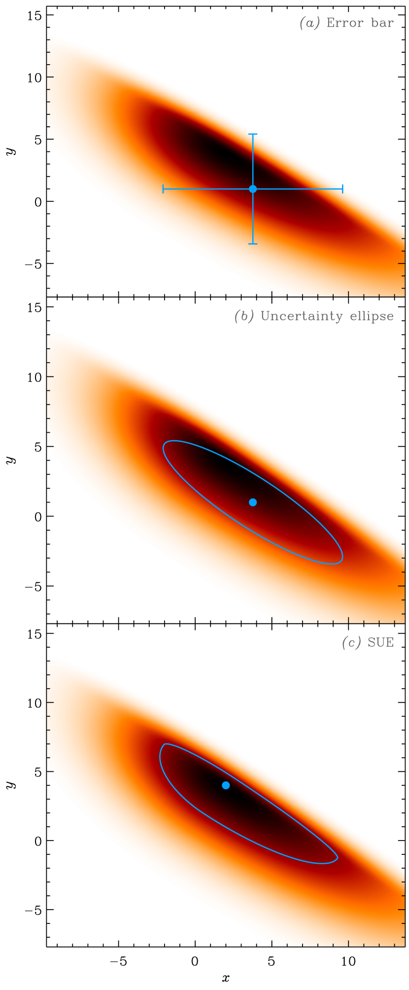
Figure 24: Uncertainty display. The orange density contours in the three panels represent an arbitrary bivariate PDF of two variables $x$ and $y$. Panel (a) shows the corresponding traditional error bar: the dot is the mean and the bars show the $\pm 1\sigma$ extent along both axes. Panel (b) shows the widely-used uncertainty ellipse, which can be viewed as the mode and $1\sigma$ contour of a bivariate normal distribution having the same means, standard-deviations and correlation coefficient as the PDF. Panel (c) shows the concept of SUE introduced in Appendix F.1.

Displaying a SUE is not straightforward. Indeed, a BSN is parametrized by its position vector, $\overrightarrow{X}_{0}=(x_{0},y_{0})$, its scale vector, $\overrightarrow{\Lambda}=(\lambda_{x},\lambda_{y})$, its shape vector, $\overrightarrow{T}=(\tau_{x},\tau_{y})$, and its rotation angle, $-\pi/2<\theta<\pi/2$. If we call $\overrightarrow{X}=(x,y)$ our original coordinates and $\overrightarrow{X^{\prime}}=(x^{\prime},y^{\prime})$ the coordinates in the centered, rotated, reference frame ($\overleftrightarrow{R}$ being the rotation matrix):

$$\overrightarrow{X^{\prime}} = \begin{array}[]{ccc}\left(\begin{array}[]{c}x^{\prime}(x,y)\\ y^{\prime}(x,y)\end{array}\right)&=&\overleftrightarrow{R}^{T}(\overrightarrow{X}-\overrightarrow{X}_{0})\end{array}$$ (25)

$$= \left(\begin{array}[]{c}(x-x_{0})\cos\theta+(y-y_{0})\sin\theta\\ -(x-x_{0})\sin\theta+(y-y_{0})\cos\theta\end{array}\right),$$ (28)

the BSN PDF can be expressed as:

$$p(x,y)=\mathcal{N}\times\left\{\begin{array}[]{l}\displaystyle\exp\left[-\frac{1}{2}\left(\frac{x^{\prime}(x,y)}{\lambda_{x}}\right)^{2}-\frac{1}{2}\left(\frac{y^{\prime}(x,y)}{\lambda_{y}}\right)^{2}\right]\\ \mbox{ if }x^{\prime}(x,y)<0\mbox{ and }y^{\prime}(x,y)<0\\ \\ \displaystyle\exp\left[-\frac{1}{2}\left(\frac{x^{\prime}(x,y)}{\lambda_{x}\tau_{x}}\right)^{2}-\frac{1}{2}\left(\frac{y^{\prime}(x,y)}{\lambda_{y}}\right)^{2}\right]\\ \mbox{ if }x^{\prime}(x,y)\geq 0\mbox{ and }y^{\prime}(x,y)<0\\ \\ \displaystyle\exp\left[-\frac{1}{2}\left(\frac{x^{\prime}(x,y)}{\lambda_{x}}\right)^{2}-\frac{1}{2}\left(\frac{y^{\prime}(x,y)}{\lambda_{y}\tau_{y}}\right)^{2}\right]\\ \mbox{ if }x^{\prime}(x,y)<0\mbox{ and }y^{\prime}(x,y)\geq 0\\ \\ \displaystyle\exp\left[-\frac{1}{2}\left(\frac{x^{\prime}(x,y)}{\lambda_{x}\tau_{x}}\right)^{2}-\frac{1}{2}\left(\frac{y^{\prime}(x,y)}{\lambda_{y}\tau_{y}}\right)^{2}\right]\\ \mbox{ if }x^{\prime}(x,y)\geq 0\mbox{ and }y^{\prime}(x,y)\geq 0,\end{array}\right.$$ (29)

where the normalization constant is:

$$\mathcal{N}=\frac{2}{\pi\lambda_{x}\lambda_{y}(1+\tau_{x})(1+\tau_{y})}.$$ (30)

We start by estimating the means ($\langle x\rangle,\langle y\rangle$), standard-deviations ($\sigma_{x},\sigma_{y}$), skewnesses ($\gamma_{x},\gamma_{y}$) and the correlation coefficient ($\rho$) of the posterior. We detail how we estimate these moments in Appendix F.2. These moments can be expressed as a function of the BSN’s parameters ($x_{0}$, $y_{0}$, $\lambda_{x}$, $\lambda_{y}$, $\tau_{x}$, $\tau_{y}$, $\theta$):

$$\langle x\rangle = \sqrt{\frac{2}{\pi}}\left[\lambda_{x}(\tau_{x}-1)\cos\theta-\lambda_{y}(\tau_{y}-1)\sin\theta\right]+x_{0}$$ (31)

$$\langle y\rangle = \sqrt{\frac{2}{\pi}}\left[\lambda_{x}(\tau_{x}-1)\sin\theta+\lambda_{y}(\tau_{y}-1)\cos\theta\right]+y_{0}$$ (32)

$$\sigma_{x}^{2} = \lambda_{x}^{2}B(\tau_{x})\cos^{2}\theta+\lambda_{y}^{2}B(\tau_{y})\sin^{2}\theta$$ (33)

$$\sigma_{y}^{2} = \lambda_{x}^{2}B(\tau_{x})\sin^{2}\theta+\lambda_{y}^{2}B(\tau_{y})\cos^{2}\theta$$ (34)

$$\rho\sigma_{x}\sigma_{y} = \left(\lambda_{x}^{2}B(\tau_{x})-\lambda_{y}^{2}B(\tau_{y})\right)\cos\theta\sin\theta$$ (35)

$$\gamma_{x}\sigma_{x}^{3} = \sqrt{\frac{2}{\pi}}\left(\lambda_{x}^{3}C(\tau_{x})\cos^{3}\theta-\lambda_{y}^{3}C(\tau_{y})\sin^{3}\theta\right)$$ (36)

$$\gamma_{y}\sigma_{y}^{3} = \sqrt{\frac{2}{\pi}}\left(\lambda_{x}^{3}C(\tau_{x})\sin^{3}\theta+\lambda_{y}^{3}C(\tau_{y})\cos^{3}\theta\right),$$ (37)

with:

$$B(\tau) = \left(1-\frac{2}{\pi}\right)(\tau-1)^{2}+\tau$$ (38)

$$C(\tau) = \left[\left(\frac{4}{\pi}-1\right)\tau^{2}+\left(3-\frac{8}{\pi}\right)\tau+\frac{4}{\pi}-1\right](\tau-1).$$ (39)

We then simply need to solve the system of Eqs. (31) – (37). To do that, we first solve $\theta$:

$$\theta=\frac{1}{2}\arctan\left(\frac{2\rho\sigma_{x}\sigma_{y}}{\sigma_{x}^{2}-\sigma_{y}^{2}}\right).$$ (40)

We then solve numerically for $\tau_{x}$ and $\tau_{y}$, independently, from the two equations:

$$\frac{C(\tau_{x})}{B(\tau_{x})^{3/2}} = \sqrt{\frac{\pi}{2}}\frac{\gamma_{x}\sigma_{x}^{3}\cos^{3}\theta+\gamma_{x}\sigma_{x}^{3}\sin^{3}\theta}{\cos^{6}\theta+\sin^{6}\theta}$$ (41)

$$\times \left(\frac{\cos^{2}\theta-\sin^{2}\theta}{\sigma_{x}^{2}\cos^{2}\theta-\sigma_{y}^{2}\sin^{2}\theta}\right)^{3/2}$$

$$\frac{C(\tau_{y})}{B(\tau_{y})^{3/2}} = \sqrt{\frac{\pi}{2}}\frac{\gamma_{y}\sigma_{y}^{3}\cos^{3}\theta-\gamma_{x}\sigma_{x}^{3}\sin^{3}\theta}{\cos^{6}\theta+\sin^{6}\theta}$$ (42)

$$\times \left(\frac{\cos^{2}\theta-\sin^{2}\theta}{\sigma_{y}^{2}\cos^{2}\theta-\sigma_{x}^{2}\sin^{2}\theta}\right)^{3/2}.$$

We derive the remaining parameters, using the following equations:

$$\lambda_{x} = \sqrt{\frac{1}{B(\tau_{x})}\frac{\sigma_{x}^{2}\cos^{2}\theta-\sigma_{y}^{2}\sin^{2}\theta}{\cos^{2}\theta-\sin^{2}\theta}}$$ (43)

$$\lambda_{y} = \sqrt{\frac{1}{B(\tau_{y})}\frac{\sigma_{y}^{2}\cos^{2}\theta-\sigma_{x}^{2}\sin^{2}\theta}{\cos^{2}\theta-\sin^{2}\theta}}$$ (44)

$$x_{0} = \langle x\rangle-\sqrt{\frac{2}{\pi}}\left[\lambda_{x}(\tau_{x}-1)\cos\theta-\lambda_{y}(\tau_{y}-1)\sin\theta\right]$$ (45)

$$y_{0} = \langle y\rangle-\sqrt{\frac{2}{\pi}}\left[\lambda_{x}(\tau_{x}-1)\sin\theta+\lambda_{y}(\tau_{y}-1)\cos\theta\right].$$ (46)

F.2 Robust Estimate of the Posterior Distribution Moments

We estimate the moments of Eqs. (31) – (37) numerically, from the marginalized posterior. Some outliers can be present due to incomplete burn-in removal, requiring robust estimators. We choose M-estimators (Mosteller & Tukey, 1977), which are a generalization of maximum-likelihood estimators. They have been popularized in astrophysics by Beers et al. (1990). Location and scale M-estimators, using Tukey’s biweight loss function were presented by Lax (1975). Posing $u_{i}=(x_{i}-l_{x})/(c\times s_{x})$, where $l_{x}=\textnormal{med}(X)$ is the median of the sample $X=\{x_{i}\}_{i=1\ldots N}$, $s_{x}=1.4826\times\textnormal{med}(|X-\textnormal{med}(X)|)$ is the Median Absolute Deviation (MAD) of $X$, and $c$ is a tuning parameter, the M-estimator of the mean is:

$$\hat{\mu}(X)=l_{x}+\frac{\sum_{|u_{i}|<1}(x_{i}-l_{x})(1-u_{i}^{2})^{2}}{\sum_{|u_{i}|<1}(1-u_{i}^{2})^{2}},$$ (47)

and for the variance:

$$\hat{V}(X)=\frac{N\times\sum_{|u_{i}|<1}(x_{i}-l_{x})^{2}(1-u_{i}^{2})^{4}}{\left[\sum_{|u_{i}|<1}(1-u_{i}^{2})(1-5u_{i}^{2})\right]\left[\sum_{|u_{i}|<1}(1-u_{i}^{2})(1-5u_{i}^{2})-1\right]}.$$ (48)

Considering a second sample $Y=\{y_{i}\}_{i=1\ldots N}$, an M-estimator of the covariance is presented by Mosteller & Tukey (1977). Posing $v_{i}=(y_{i}-l_{y})/(c\times s_{y})$, the covariance can be estimated as:

$$\hat{V}(X,Y)=\frac{N\times\sum_{|u_{i}|<1,|v_{i}|<1}(x_{i}-l_{x})(1-u_{i}^{2})^{2}(y_{i}-l_{y})(1-v_{i}^{2})^{2}}{\left[\sum_{|u_{i}|<1}(1-u_{i}^{2})(1-5u_{i}^{2})\right]\left[\sum_{|v_{i}|<1}(1-v_{i}^{2})(1-5v_{i}^{2})\right]}.$$ (49)

These estimators are implemented in the Python astropy module (Astropy Collaboration et al., 2013, 2018). We have designed our own skewness W-estimator:

$$\hat{\gamma}(X)=\frac{\sum_{|u_{i}|<1}u_{i}^{3}(1-u_{i}^{2})^{2}}{\sum_{|u_{i}|<1}(1-u_{i}^{2})^{2}}.$$ (50)

We have also slightly improved astropy’s implementation by iterating on Eqs. (47) – (50), replacing $l_{x}$, $l_{y}$, $s_{x}$ and $s_{y}$ with $\hat{\mu}(X)$, $\hat{\mu}(Y)$, $\sqrt{\hat{V}(X)}$ and $\sqrt{\hat{V}(Y)}$, respectively, until a $10^{-5}$ relative accuracy is reached. The tuning parameter is usually taken as $c=6$ for the mean and $c=9$ for the variance, covariance and skewness.

Appendix G DUST EVOLUTION RESULTS ASSUMING A CHABRIER IMF

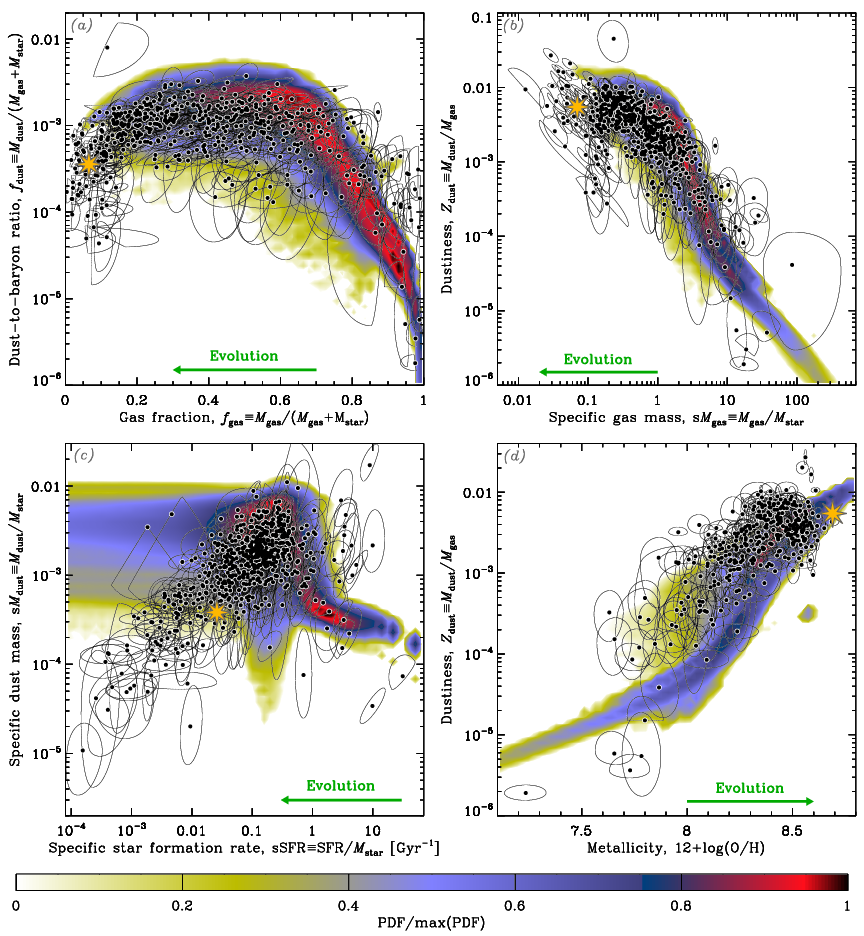
Figure 25: Fitted dust evolution tracks, assuming a Chabrier (2003) IMF. This is the equivalent of Fig. 14.

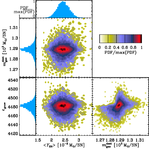
Figure 26: Posterior distribution of the tuning parameters, assuming a Chabrier (2003) IMF. This is the equivalent of Fig. 16.

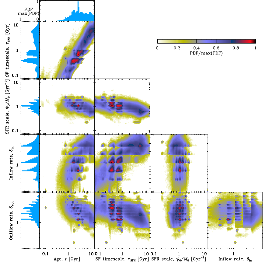
Figure 27: Posterior distribution of the SFH-related parameters, assuming a Chabrier (2003) IMF. This is the equivalent of Fig. 17.

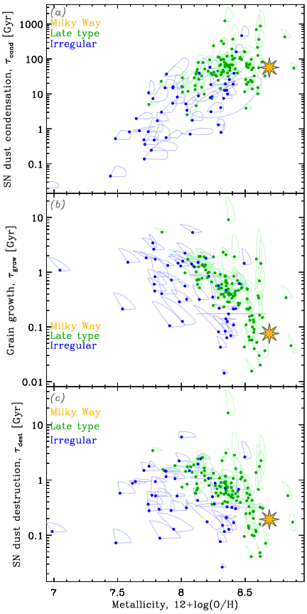
Figure 28: Posterior distribution of the tuning parameters, assuming a Chabrier (2003) IMF. This is the equivalent of Fig. 18.

We have performed the modelling of Sect. 5.2.2, assuming a Chabrier (2003) IMF. The data have been corrected accordingly: $M_{\star}$ has been multiplied by 0.61 and SFR by 0.63 (Madau & Dickinson, 2014), as these two quantities were derived assuming a Salpeter (1955) IMF. Fig. 25 shows the fit of the scaling relations; it is the equivalent of Fig. 14. Figs. 26 – 27 display the PDF of the dust evolution and SFH-related parameters, respectively; they are the equivalent of Figs. 16 – 17. The inferred timescales are displayed in Fig. 28; it is the equivalent of Fig. 18.

Appendix H REFERENCE RUN PARAMETERS

Table H gives the mean and standard-deviation of the most relevant parameters derived with the reference run (cf. Sect. 3.2), for each galaxy of the sample presented in Sect. 2.

[c]l—*3r—*5r Main inferred quantities for each galaxy, with the reference run. For each quantity, we quote the mean $\pm$ the standard-deviation of the posterior PDF.
Galaxy $\log M_{\mbox{{\scriptsize dust}}}/M_{\odot}$ $\log\langle U\rangle$ $\log q_{\mbox{{\scriptsize AF}}}$ $\log M_{\mbox{{\scriptsize gas}}}/M_{\odot}$ $\log f_{\mbox{{\scriptsize H${}_{\textnormal{2}}$}}}$ $\log M_{\star}/M_{\odot}$ $\log\textnormal{sSFR}/\textnormal{yr}^{-1}$ $12+\log(\textnormal{O/H})$
continued.
Galaxy $\log M_{\mbox{{\scriptsize dust}}}/M_{\odot}$ $\log\langle U\rangle$ $\log q_{\mbox{{\scriptsize AF}}}$ $\log M_{\mbox{{\scriptsize gas}}}/M_{\odot}$ $\log f_{\mbox{{\scriptsize H${}_{\textnormal{2}}$}}}$ $\log M_{\star}/M_{\odot}$ $\log\textnormal{sSFR}/\textnormal{yr}^{-1}$ $12+\log(\textnormal{O/H})$
ESO 149-013 $5.4\pm 0.5$ $-0.4\pm 0.5$ $-1.10\pm 0.21$ $8.864\pm 0.023$ … $8.42\pm 0.19$ … …
NGC 0007 $6.20\pm 0.17$ $0.13\pm 0.18$ $-1.22\pm 0.11$ $9.31\pm 0.03$ … $9.06\pm 0.10$ $-9.75\pm 0.11$ …
ESO 410-005 $3.5\pm 0.5$ $0.4\pm 0.8$ $-1.4\pm 0.4$ … … $6.28\pm 0.14$ … …
IC 0010 $5.61\pm 0.20$ $0.47\pm 0.19$ $-1.25\pm 0.16$ $8.08\pm 0.06$ … $8.66\pm 0.12$ $-9.99\pm 0.31$ $8.18\pm 0.09$
NGC 0115 $6.80\pm 0.12$ $0.02\pm 0.13$ $-1.22\pm 0.08$ $9.67\pm 0.04$ … $9.48\pm 0.10$ $-9.78\pm 0.10$ …
ESO 410-012 $5.4\pm 0.5$ $-0.3\pm 0.5$ $-1.11\pm 0.21$ $8.915\pm 0.029$ … $8.13\pm 0.13$ $-9.73\pm 0.14$ …
NGC 0131 $6.63\pm 0.07$ $0.12\pm 0.07$ $-0.99\pm 0.04$ $9.408\pm 0.005$ … $9.30\pm 0.09$ $-10.01\pm 0.11$ …
UGC 00300 $5.1\pm 0.4$ $-0.0\pm 0.4$ $-1.35\pm 0.16$ $8.391\pm 0.022$ … $8.34\pm 0.12$ $-10.02\pm 0.13$ $8.00\pm 0.05$
UGC 00313 $6.51\pm 0.13$ $0.24\pm 0.14$ $-1.10\pm 0.07$ $8.54\pm 0.06$ … $9.30\pm 0.08$ $-10.00\pm 0.11$ $8.34\pm 0.08$
ESO 410-018 $6.31\pm 0.16$ $-0.16\pm 0.20$ $-1.00\pm 0.11$ $9.31\pm 0.07$ … $8.82\pm 0.11$ $-9.60\pm 0.11$ …
NGC 0148 $5.95\pm 0.25$ $0.32\pm 0.31$ $-0.92\pm 0.14$ … … $10.55\pm 0.05$ … …
NGC 0150 $7.225\pm 0.020$ $0.682\pm 0.016$ $-1.096\pm 0.007$ $9.90\pm 0.04$ … $10.13\pm 0.08$ $-9.74\pm 0.10$ …
ESO 411-013 $5.9\pm 0.3$ $-0.1\pm 0.4$ $-0.99\pm 0.17$ … … $8.86\pm 0.12$ $-10.48\pm 0.24$ …
NGC 0254 $5.94\pm 0.20$ $0.19\pm 0.27$ $-0.95\pm 0.13$ … … $10.23\pm 0.07$ $-11.9\pm 0.4$ …
ESO 411-016 $5.77\pm 0.24$ $0.33\pm 0.26$ $-1.16\pm 0.13$ $8.61\pm 0.10$ … $8.64\pm 0.13$ $-9.75\pm 0.14$ …
NGC 0289 $7.51\pm 0.04$ $0.30\pm 0.04$ $-0.957\pm 0.029$ $10.530\pm 0.015$ … $10.52\pm 0.07$ $-10.16\pm 0.09$ $8.597\pm 0.011$
ESO 411-026 $5.6\pm 0.4$ $-0.1\pm 0.5$ $-1.12\pm 0.20$ … … $8.37\pm 0.16$ $-10.01\pm 0.19$ …
ESO 411-027 $5.9\pm 0.4$ $-0.2\pm 0.4$ $-1.06\pm 0.20$ … … $8.37\pm 0.25$ $-9.82\pm 0.27$ …
NGC 0300 $6.93\pm 0.05$ $-0.56\pm 0.07$ $-0.94\pm 0.05$ $9.41\pm 0.03$ … $9.20\pm 0.10$ $-9.90\pm 0.12$ $8.257\pm 0.010$
NGC 0337 $7.08\pm 0.06$ $0.65\pm 0.05$ $-1.21\pm 0.05$ $9.726\pm 0.022$ … $9.67\pm 0.08$ $-9.37\pm 0.09$ $8.33\pm 0.06$
ESO 351-030 $0.3\pm 0.4$ $-0.7\pm 0.4$ $-0.8\pm 0.5$ $5.557\pm 0.004$ … $2.33\pm 0.29$ … …
IC 1613 $4.34\pm 0.16$ $0.27\pm 0.30$ $-1.42\pm 0.17$ $7.7941\pm 0.0028$ … $7.68\pm 0.10$ $-9.96\pm 0.11$ $7.95\pm 0.06$
NGC 0428 $6.85\pm 0.08$ $0.12\pm 0.08$ $-1.19\pm 0.07$ $9.7269\pm 0.0011$ … $9.52\pm 0.05$ $-9.66\pm 0.06$ $8.224\pm 0.028$
UGC 00772 $5.1\pm 0.5$ $-0.3\pm 0.6$ $-1.12\pm 0.25$ $8.572\pm 0.007$ … $7.68\pm 0.24$ $-9.26\pm 0.24$ …
NGC 0448 $6.16\pm 0.22$ $0.35\pm 0.26$ $-1.00\pm 0.11$ … … $10.40\pm 0.07$ … …
NGC 0493 $7.21\pm 0.06$ $0.13\pm 0.06$ $-1.085\pm 0.031$ $9.6285\pm 0.0027$ … $9.60\pm 0.07$ $-9.70\pm 0.09$ $8.315\pm 0.023$
UGC 00931 $6.3\pm 0.3$ $0.1\pm 0.3$ $-1.30\pm 0.17$ $9.17\pm 0.06$ … $8.66\pm 0.14$ $-9.81\pm 0.21$ $8.03\pm 0.07$
NGC 0520 $7.45\pm 0.06$ $1.14\pm 0.06$ $-1.308\pm 0.009$ … … $10.35\pm 0.06$ $-9.43\pm 0.07$ …
NGC 0584 $6.07\pm 0.20$ $0.84\pm 0.25$ $-0.94\pm 0.13$ … … $10.97\pm 0.04$ $-12.7\pm 0.4$ …
NGC 0586 $6.58\pm 0.09$ $0.08\pm 0.10$ $-0.87\pm 0.06$ … … $9.90\pm 0.06$ $-11.31\pm 0.31$ …
NGC 0613 $8.010\pm 0.017$ $0.612\pm 0.021$ $-1.019\pm 0.011$ $10.37\pm 0.12$ $-0.47\pm 0.19$ $10.90\pm 0.09$ $-9.86\pm 0.13$ $8.564\pm 0.022$
NGC 0625 $5.63\pm 0.12$ $0.61\pm 0.10$ $-1.29\pm 0.07$ $8.426\pm 0.023$ … $8.52\pm 0.10$ $-9.79\pm 0.13$ $8.039\pm 0.015$
NGC 0628 $7.64\pm 0.07$ $0.18\pm 0.09$ $-0.81\pm 0.04$ $10.460\pm 0.005$ $-1.41\pm 0.15$ $10.14\pm 0.06$ $-9.79\pm 0.10$ $8.481\pm 0.006$
NGC 0678 $7.19\pm 0.10$ $-0.15\pm 0.10$ $-0.70\pm 0.06$ $9.96\pm 0.11$ … $10.78\pm 0.05$ $-11.5\pm 0.4$ …
NGC 0720 $6.3\pm 0.4$ $0.6\pm 0.4$ $-0.69\pm 0.21$ … … $11.37\pm 0.04$ $-13.0\pm 0.4$ …
PGC 007045 $6.27\pm 0.09$ $0.17\pm 0.10$ $-0.92\pm 0.05$ … … $9.58\pm 0.06$ $-11.1\pm 0.4$ …
NGC 0855 $5.58\pm 0.09$ $0.66\pm 0.09$ $-1.10\pm 0.07$ $8.281\pm 0.030$ … $8.97\pm 0.08$ $-10.74\pm 0.21$ …
PGC 008962 $5.8\pm 0.3$ $0.1\pm 0.3$ $-1.32\pm 0.16$ $9.194\pm 0.028$ … $8.67\pm 0.15$ $-9.70\pm 0.16$ $8.06\pm 0.08$
NGC 0895 $7.75\pm 0.04$ $0.05\pm 0.04$ $-0.869\pm 0.011$ $10.277\pm 0.019$ … $10.29\pm 0.07$ $-9.83\pm 0.09$ $8.431\pm 0.031$
NGC 0891 $7.744\pm 0.008$ $0.487\pm 0.013$ $-1.021\pm 0.013$ $10.01\pm 0.05$ $-0.62\pm 0.14$ $10.49\pm 0.11$ $-10.34\pm 0.30$ …
NGC 0925 $7.47\pm 0.06$ $-0.29\pm 0.07$ $-0.95\pm 0.07$ $10.0670\pm 0.0021$ $-1.76\pm 0.14$ $9.67\pm 0.09$ $-9.61\pm 0.09$ $8.303\pm 0.012$
PGC 009485 $6.60\pm 0.23$ $0.90\pm 0.24$ $-1.10\pm 0.06$ … … $9.94\pm 0.07$ $-9.84\pm 0.12$ …
NGC 1056 $7.25\pm 0.03$ $0.72\pm 0.04$ $-1.003\pm 0.019$ $9.974\pm 0.021$ … $10.31\pm 0.08$ $-10.03\pm 0.14$ $8.44\pm 0.04$
NGC 1097 $7.776\pm 0.019$ $0.585\pm 0.021$ $-1.011\pm 0.010$ $10.26\pm 0.07$ $-0.48\pm 0.14$ $10.84\pm 0.08$ $-10.04\pm 0.10$ $8.55\pm 0.04$
NGC 1140 $6.34\pm 0.09$ $0.91\pm 0.09$ $-1.29\pm 0.07$ $9.550\pm 0.016$ $-2.12\pm 0.17$ $9.10\pm 0.11$ $-9.10\pm 0.11$ $8.25\pm 0.08$
PGC 166069 $5.3\pm 0.4$ $-0.2\pm 0.3$ $-1.01\pm 0.16$ $7.8\pm 0.5$ … $7.98\pm 0.17$ … …
UGC 02392 $6.28\pm 0.17$ $0.07\pm 0.20$ $-0.99\pm 0.11$ $9.130\pm 0.008$ … $9.44\pm 0.10$ $-10.43\pm 0.13$ …
NGC 1189 $7.02\pm 0.13$ $-0.14\pm 0.15$ $-0.98\pm 0.07$ … … $9.62\pm 0.10$ $-10.08\pm 0.12$ …
NGC 1222 $6.817\pm 0.019$ $1.470\pm 0.019$ $-1.297\pm 0.013$ $9.48\pm 0.05$ … $9.78\pm 0.09$ $-9.03\pm 0.11$ …
PGC 166071 $6.6\pm 0.5$ $0.4\pm 0.4$ $-0.96\pm 0.15$ … … $10.40\pm 0.15$ … …
ESO 116-012 $7.18\pm 0.29$ $0.01\pm 0.26$ $-0.57\pm 0.04$ … … … … …
NGC 1266 $6.60\pm 0.03$ $1.54\pm 0.03$ $-1.892\pm 0.010$ … … $9.96\pm 0.10$ $-9.58\pm 0.11$ …
PGC 012608 $5.97\pm 0.30$ $0.04\pm 0.31$ $-1.05\pm 0.15$ … … $9.00\pm 0.13$ $-9.92\pm 0.15$ …
NGC 1317 $6.636\pm 0.027$ $0.64\pm 0.03$ $-0.924\pm 0.014$ … … $10.41\pm 0.07$ $-11.06\pm 0.16$ …
NGC 1336 $5.87\pm 0.26$ $-0.05\pm 0.27$ $-0.94\pm 0.13$ … … $9.90\pm 0.07$ $-11.7\pm 0.4$ …
ESO 358-006 $5.5\pm 0.4$ $0.0\pm 0.5$ $-0.83\pm 0.26$ … … $8.17\pm 0.15$ $-9.95\pm 0.17$ …
NGC 1351A $6.84\pm 0.07$ $-0.23\pm 0.08$ $-0.88\pm 0.04$ $8.91\pm 0.09$ $-0.89\pm 0.15$ $9.47\pm 0.08$ $-10.61\pm 0.16$ …
NGC 1351 $6.1\pm 0.3$ $0.1\pm 0.3$ $-0.86\pm 0.15$ … … $10.49\pm 0.08$ $-12.2\pm 0.3$ …
PGC 013058 $5.73\pm 0.18$ $0.18\pm 0.20$ $-1.00\pm 0.10$ … … $8.85\pm 0.09$ $-10.61\pm 0.22$ …
PGC 013084 $5.4\pm 0.4$ $-0.4\pm 0.4$ $-0.90\pm 0.16$ … … $9.35\pm 0.08$ $-11.57\pm 0.17$ …
PGC 013097 $5.5\pm 0.3$ $0.1\pm 0.4$ $-1.04\pm 0.20$ … … $8.86\pm 0.10$ $-11.2\pm 0.5$ …
PGC 013146 $5.3\pm 0.4$ $-0.2\pm 0.4$ $-0.97\pm 0.18$ … … $9.10\pm 0.09$ $-11.5\pm 0.3$ …
ESO 358-015 $5.2\pm 0.3$ $0.1\pm 0.4$ $-1.07\pm 0.17$ $8.30\pm 0.05$ … $8.39\pm 0.13$ $-10.15\pm 0.16$ …
ESO 358-016 $5.8\pm 0.4$ $-0.0\pm 0.4$ $-1.06\pm 0.17$ … … $8.37\pm 0.16$ $-10.08\pm 0.21$ …
NGC 1365 $8.018\pm 0.020$ $0.72\pm 0.03$ $-1.163\pm 0.019$ $10.40\pm 0.07$ $-0.41\pm 0.14$ $10.81\pm 0.09$ $-9.76\pm 0.19$ $8.551\pm 0.012$
PGC 013230 $5.5\pm 0.4$ $-0.3\pm 0.4$ $-0.94\pm 0.18$ … … $9.14\pm 0.09$ $-11.6\pm 0.5$ …
ESO 358-019 $5.7\pm 0.5$ $-0.4\pm 0.5$ $-1.07\pm 0.22$ … … $8.38\pm 0.19$ … …
NGC 1373 $5.4\pm 0.4$ $-0.3\pm 0.4$ $-0.89\pm 0.17$ … … $9.57\pm 0.06$ $-12.2\pm 0.4$ …
NGC 1374 $5.48\pm 0.26$ $0.38\pm 0.26$ $-0.86\pm 0.09$ … … $10.57\pm 0.05$ $-12.79\pm 0.17$ …
IC 0335 $5.75\pm 0.29$ $0.01\pm 0.31$ $-0.87\pm 0.15$ … … $10.24\pm 0.07$ $-12.4\pm 0.4$ …
NGC 1379 $5.84\pm 0.26$ $0.3\pm 0.3$ $-0.89\pm 0.15$ … … $10.57\pm 0.07$ $-12.6\pm 0.4$ …
NGC 1381 $5.6\pm 0.3$ $0.4\pm 0.4$ $-0.78\pm 0.20$ … … $10.60\pm 0.03$ $-12.8\pm 0.4$ …
NGC 1369 $5.3\pm 0.4$ $-0.3\pm 0.4$ $-0.90\pm 0.16$ … … $9.85\pm 0.06$ $-12.4\pm 0.3$ …
NGC 1386 $6.645\pm 0.016$ $0.837\pm 0.016$ $-0.967\pm 0.006$ … … $10.25\pm 0.08$ $-11.0\pm 0.4$ $8.56\pm 0.04$
NGC 1380A $5.73\pm 0.25$ $0.14\pm 0.28$ $-0.92\pm 0.13$ … … $9.98\pm 0.04$ $-12.0\pm 0.4$ …
PGC 013343 $5.77\pm 0.29$ $-0.3\pm 0.3$ $-0.87\pm 0.15$ … … $9.22\pm 0.08$ $-11.7\pm 0.4$ …
NGC 1387 $6.36\pm 0.06$ $0.84\pm 0.05$ $-1.06\pm 0.04$ … … $10.83\pm 0.07$ $-11.96\pm 0.27$ …
NGC 1389 $6.07\pm 0.28$ $0.2\pm 0.3$ $-0.85\pm 0.15$ … … $10.54\pm 0.09$ $-12.48\pm 0.29$ …
ESO 358-042 $5.1\pm 0.5$ $-0.5\pm 0.5$ $-1.07\pm 0.21$ … … $8.94\pm 0.10$ … …
ESO 358-043 $6.01\pm 0.26$ $-0.27\pm 0.29$ $-0.96\pm 0.14$ … … $9.28\pm 0.08$ $-11.1\pm 0.5$ …
NGC 1399 $6.0\pm 0.6$ $0.7\pm 0.6$ $-0.5\pm 0.4$ … … $11.45\pm 0.10$ $-12.25\pm 0.21$ …
NGC 1404 $5.74\pm 0.30$ $0.59\pm 0.30$ $-0.71\pm 0.05$ … … $11.12\pm 0.04$ $-12.98\pm 0.22$ …
NGC 1427A $6.23\pm 0.12$ $-0.05\pm 0.13$ $-1.30\pm 0.08$ $9.33\pm 0.05$ … $8.97\pm 0.09$ $-9.79\pm 0.11$ $8.129\pm 0.008$
NGC 1412 $5.39\pm 0.25$ $0.70\pm 0.26$ $-1.02\pm 0.13$ $9.24\pm 0.12$ … $10.11\pm 0.06$ $-11.7\pm 0.5$ …
NGC 1419 $5.70\pm 0.30$ $-0.08\pm 0.31$ $-0.91\pm 0.14$ … … $10.06\pm 0.07$ $-12.16\pm 0.29$ …
ESO 358-050 $5.69\pm 0.28$ $-0.09\pm 0.29$ $-0.96\pm 0.13$ … … $9.77\pm 0.06$ $-11.82\pm 0.25$ …
ESO 358-051 $6.09\pm 0.19$ $0.22\pm 0.18$ $-1.09\pm 0.04$ $8.33\pm 0.12$ … $8.75\pm 0.09$ $-9.90\pm 0.12$ $8.262\pm 0.008$
NGC 1427 $6.2\pm 0.4$ $0.1\pm 0.4$ $-0.86\pm 0.16$ … … $10.58\pm 0.04$ $-12.4\pm 0.4$ …
NGC 1428 $5.73\pm 0.29$ $0.03\pm 0.30$ $-0.91\pm 0.14$ … … $9.90\pm 0.04$ $-12.37\pm 0.29$ …
PGC 013635 $5.70\pm 0.20$ $-0.02\pm 0.23$ $-0.94\pm 0.12$ … … $9.05\pm 0.06$ $-10.84\pm 0.13$ …
ESO 358-054 $6.16\pm 0.15$ $-0.08\pm 0.16$ $-1.27\pm 0.09$ $8.83\pm 0.04$ … $8.75\pm 0.09$ $-9.74\pm 0.10$ $8.134\pm 0.011$
PGC 166861 $5.6\pm 0.3$ $0.7\pm 0.3$ $-1.30\pm 0.18$ … … $8.56\pm 0.22$ … …
ESO 358-056 $5.25\pm 0.29$ $0.6\pm 0.3$ $-1.15\pm 0.17$ … … $8.82\pm 0.10$ $-11.0\pm 0.5$ …
NGC 1436 $6.80\pm 0.04$ $-0.03\pm 0.05$ $-0.798\pm 0.026$ $8.40\pm 0.08$ $-0.47\pm 0.14$ $9.93\pm 0.07$ $-11.21\pm 0.21$ $8.561\pm 0.007$
UGC 02826 $6.71\pm 0.07$ $0.64\pm 0.07$ $-0.92\pm 0.03$ … … $10.01\pm 0.09$ $-10.68\pm 0.23$ …
ESO 358-059 $5.3\pm 0.4$ $-0.2\pm 0.4$ $-0.94\pm 0.16$ … … $9.68\pm 0.08$ $-11.9\pm 0.5$ …
ESO 358-060 $5.1\pm 0.6$ $-0.0\pm 0.5$ $-1.48\pm 0.24$ $7.947\pm 0.026$ … $7.60\pm 0.30$ $-9.14\pm 0.30$ $7.89\pm 0.16$
PGC 166077 $5.14\pm 0.27$ $-0.6\pm 0.3$ $-1.10\pm 0.20$ $6.47\pm 0.09$ … $7.11\pm 0.20$ $-9.26\pm 0.21$ …
NGC 1437B $6.23\pm 0.08$ $-0.20\pm 0.09$ $-0.90\pm 0.04$ … … $8.75\pm 0.10$ $-10.52\pm 0.26$ …
ESO 358-063 $7.053\pm 0.031$ $0.308\pm 0.028$ $-0.890\pm 0.013$ $9.38\pm 0.05$ $-0.66\pm 0.14$ $9.82\pm 0.08$ $-10.20\pm 0.16$ …
IC 0342 $7.50\pm 0.05$ $0.44\pm 0.05$ $-0.910\pm 0.025$ … … $10.28\pm 0.07$ $-9.68\pm 0.08$ $8.55\pm 0.06$
ESO 358-066 $5.5\pm 0.4$ $-0.1\pm 0.4$ $-1.09\pm 0.19$ … … $8.79\pm 0.12$ … …
ESO 359-002 $5.7\pm 0.4$ $-0.0\pm 0.4$ $-0.98\pm 0.17$ … … $9.33\pm 0.16$ $-11.2\pm 0.4$ …
NGC 1482 $7.073\pm 0.012$ $1.197\pm 0.010$ $-1.113\pm 0.007$ … … $9.94\pm 0.09$ $-9.24\pm 0.10$ …
ESO 549-035 $6.38\pm 0.20$ $-0.04\pm 0.25$ $-1.08\pm 0.13$ $9.19\pm 0.05$ … $9.10\pm 0.11$ $-9.85\pm 0.13$ …
NGC 1510 $5.67\pm 0.20$ $0.61\pm 0.20$ $-1.15\pm 0.10$ … … $8.79\pm 0.11$ $-9.75\pm 0.12$ $8.22\pm 0.10$
NGC 1566 $6.759\pm 0.029$ $0.60\pm 0.06$ $-0.95\pm 0.05$ $9.60\pm 0.11$ $-0.48\pm 0.19$ $9.73\pm 0.11$ $-9.92\pm 0.13$ $8.584\pm 0.016$
UGC 03016 $6.82\pm 0.12$ $0.24\pm 0.14$ $-0.89\pm 0.08$ $9.08\pm 0.26$ … $9.86\pm 0.11$ … …
NGC 1569 $5.46\pm 0.14$ $1.46\pm 0.14$ $-1.63\pm 0.06$ $8.326\pm 0.022$ $-1.40\pm 0.17$ $8.52\pm 0.09$ $-8.56\pm 0.10$ $7.96\pm 0.09$
IC 2085 $6.31\pm 0.08$ $-0.06\pm 0.09$ $-0.92\pm 0.04$ … … $9.25\pm 0.07$ $-10.8\pm 0.4$ …
NGC 1617 $6.76\pm 0.05$ $0.00\pm 0.05$ $-0.796\pm 0.023$ … … $10.65\pm 0.10$ $-12.4\pm 0.5$ …
ESO 157-047 $5.4\pm 0.3$ $0.3\pm 0.3$ $-1.18\pm 0.15$ $8.80\pm 0.04$ … $8.65\pm 0.13$ $-10.08\pm 0.17$ …
ESO 157-049 $7.24\pm 0.13$ $0.18\pm 0.12$ $-1.130\pm 0.018$ $9.285\pm 0.020$ … $9.51\pm 0.08$ $-9.82\pm 0.12$ $8.428\pm 0.009$
NGC 1705 $5.17\pm 0.16$ $0.57\pm 0.16$ $-1.37\pm 0.10$ $8.199\pm 0.022$ … $8.30\pm 0.10$ $-9.40\pm 0.10$ $8.086\pm 0.013$
NGC 1800 $5.51\pm 0.08$ $0.44\pm 0.08$ $-1.195\pm 0.021$ $8.380\pm 0.016$ … $8.60\pm 0.09$ $-9.87\pm 0.11$ $8.23\pm 0.06$
NGC 1808 $7.264\pm 0.028$ $1.23\pm 0.04$ $-1.209\pm 0.021$ $10.61\pm 0.12$ $-0.23\pm 0.17$ $10.42\pm 0.10$ $-9.74\pm 0.13$ …
NGC 1924 $7.20\pm 0.04$ $0.61\pm 0.04$ $-1.037\pm 0.029$ $9.56\pm 0.05$ … $10.10\pm 0.08$ $-9.88\pm 0.19$ …
NGC 2146 $8.083\pm 0.011$ $1.119\pm 0.010$ $-1.112\pm 0.005$ … … $10.94\pm 0.10$ $-9.45\pm 0.16$ …
NGC 2273 $7.095\pm 0.021$ $0.947\pm 0.020$ $-1.207\pm 0.011$ $9.71\pm 0.06$ $-0.49\pm 0.16$ $10.63\pm 0.09$ $-10.45\pm 0.19$ …
PGC 2807061 $3.3\pm 0.8$ $-0.8\pm 0.7$ $-1.2\pm 0.4$ $7.43\pm 0.06$ … $6.84\pm 0.20$ … …
UGC 03701 $6.79\pm 0.18$ $0.09\pm 0.22$ $-1.13\pm 0.10$ $9.69\pm 0.05$ … $9.57\pm 0.10$ $-9.92\pm 0.13$ $8.35\pm 0.04$
ESO 428-014 $6.15\pm 0.24$ $1.57\pm 0.23$ $-1.08\pm 0.06$ … … … … …
NGC 2403 $7.11\pm 0.06$ $0.05\pm 0.06$ $-1.061\pm 0.024$ $9.565\pm 0.022$ $-1.26\pm 0.14$ $9.45\pm 0.06$ $-9.59\pm 0.07$ $8.298\pm 0.025$
ESO 560-004 $7.22\pm 0.08$ $0.78\pm 0.08$ $-1.07\pm 0.03$ … … $10.46\pm 0.12$ … …
UGC 03960 $5.8\pm 0.3$ $0.1\pm 0.4$ $-0.93\pm 0.15$ … … $10.07\pm 0.08$ $-12.0\pm 0.4$ …
ESO 493-016 $7.53\pm 0.06$ $0.62\pm 0.06$ $-1.030\pm 0.030$ … … $9.99\pm 0.12$ $-9.08\pm 0.18$ …
ESO 209-009 $7.56\pm 0.04$ $0.07\pm 0.04$ $-0.97\pm 0.04$ $9.691\pm 0.020$ … $10.08\pm 0.10$ … …
IC 2233 $6.29\pm 0.15$ $-0.05\pm 0.14$ $-1.13\pm 0.13$ $9.46\pm 0.05$ … $9.13\pm 0.05$ $-9.82\pm 0.06$ $8.11\pm 0.05$
NGC 2549 $5.74\pm 0.22$ $0.05\pm 0.24$ $-0.87\pm 0.13$ … … $10.27\pm 0.04$ $-12.5\pm 0.4$ …
UGC 04305 $5.30\pm 0.23$ $0.16\pm 0.21$ $-1.55\pm 0.15$ $8.871\pm 0.022$ … $8.27\pm 0.10$ $-9.35\pm 0.11$ $7.82\pm 0.05$
NGC 2577 $6.06\pm 0.27$ $0.55\pm 0.28$ $-1.00\pm 0.14$ … … $10.85\pm 0.05$ … …
NGC 2592 $5.5\pm 0.4$ $-0.1\pm 0.4$ $-0.90\pm 0.16$ … … $10.464\pm 0.030$ $-12.7\pm 0.3$ …
ESO 495-021 $6.127\pm 0.018$ $1.320\pm 0.018$ $-1.219\pm 0.010$ $8.471\pm 0.021$ … $8.85\pm 0.12$ $-8.86\pm 0.15$ $8.441\pm 0.012$
UGC 04483 $4.0\pm 0.3$ $0.43\pm 0.31$ $-1.81\pm 0.18$ $7.533\pm 0.022$ … $6.16\pm 0.22$ $-8.55\pm 0.22$ $7.63\pm 0.07$
UGC 04551 $5.9\pm 0.3$ $0.1\pm 0.3$ $-0.86\pm 0.16$ … … $10.50\pm 0.04$ $-12.5\pm 0.4$ …
UGC 04549 $6.82\pm 0.09$ $0.14\pm 0.10$ $-0.89\pm 0.04$ $9.20\pm 0.04$ … $9.41\pm 0.07$ $-9.93\pm 0.10$ $8.44\pm 0.05$
NGC 2679 $5.8\pm 0.4$ $0.1\pm 0.3$ $-0.90\pm 0.17$ … … $10.36\pm 0.06$ $-12.50\pm 0.21$ …
NGC 2685 $6.81\pm 0.08$ $-0.23\pm 0.08$ $-0.58\pm 0.04$ … … $10.03\pm 0.06$ $-11.20\pm 0.14$ …
NGC 2655 $6.65\pm 0.11$ $-0.01\pm 0.09$ $-0.73\pm 0.08$ $9.66\pm 0.09$ … $10.51\pm 0.03$ $-11.63\pm 0.12$ …
UGC 04684 $6.77\pm 0.11$ $0.24\pm 0.12$ $-1.28\pm 0.06$ $9.648\pm 0.005$ … $9.53\pm 0.10$ $-9.73\pm 0.11$ $8.31\pm 0.06$
NGC 2764 $7.30\pm 0.03$ $0.67\pm 0.03$ $-0.994\pm 0.013$ … … $10.03\pm 0.07$ $-9.83\pm 0.12$ …
NGC 2768 $6.4\pm 0.3$ $0.25\pm 0.30$ $-0.68\pm 0.13$ … … $11.20\pm 0.09$ $-12.80\pm 0.28$ …
NGC 2778 $5.41\pm 0.27$ $0.1\pm 0.3$ $-0.96\pm 0.15$ … … $10.22\pm 0.05$ $-12.23\pm 0.22$ …
NGC 2787 $5.56\pm 0.27$ $0.28\pm 0.24$ $-1.00\pm 0.13$ $9.36\pm 0.13$ … $10.16\pm 0.05$ $-11.5\pm 0.5$ …
IC 2461 $7.56\pm 0.04$ $0.34\pm 0.05$ $-1.019\pm 0.027$ $10.01\pm 0.04$ … $10.42\pm 0.08$ $-10.44\pm 0.30$ …
NGC 2841 $7.83\pm 0.05$ $0.07\pm 0.08$ $-0.69\pm 0.12$ $10.193\pm 0.022$ … $11.27\pm 0.05$ $-11.22\pm 0.11$ $8.69\pm 0.03$
NGC 2853 $6.70\pm 0.10$ $0.04\pm 0.11$ $-0.93\pm 0.06$ … … $9.42\pm 0.08$ $-10.01\pm 0.09$ $8.45\pm 0.05$
NGC 2859 $6.91\pm 0.20$ $-0.29\pm 0.18$ $-0.75\pm 0.11$ $10.19\pm 0.18$ … $10.87\pm 0.04$ $-12.1\pm 0.4$ …
NGC 2915 $5.06\pm 0.17$ $0.41\pm 0.16$ $-1.35\pm 0.12$ $8.700\pm 0.030$ … $8.39\pm 0.09$ $-9.73\pm 0.10$ $8.123\pm 0.009$
NGC 2907 $7.03\pm 0.12$ $-0.07\pm 0.13$ $-0.83\pm 0.10$ $10.17\pm 0.15$ … $10.98\pm 0.06$ $-11.6\pm 0.4$ …
PGC 027066 $6.87\pm 0.24$ $0.06\pm 0.28$ $-0.96\pm 0.13$ … … $9.52\pm 0.15$ $-10.57\pm 0.30$ …
ESO 373-008 $7.05\pm 0.05$ $-0.25\pm 0.09$ $-0.97\pm 0.07$ $9.164\pm 0.021$ … $9.41\pm 0.11$ … …
UGC 05139 $4.6\pm 0.4$ $-0.1\pm 0.3$ $-1.45\pm 0.18$ $8.213\pm 0.022$ … $7.53\pm 0.15$ $-9.47\pm 0.15$ $7.92\pm 0.08$
NGC 2974 $7.16\pm 0.12$ $-0.16\pm 0.12$ $-0.338\pm 0.031$ … … … … …
NGC 2950 $5.0\pm 0.6$ $1.1\pm 0.6$ $-1.41\pm 0.18$ … … $10.532\pm 0.023$ $-12.14\pm 0.09$ …
PGC 090942 $5.7\pm 0.6$ $-0.7\pm 0.5$ $-1.02\pm 0.23$ $9.802\pm 0.025$ … $9.0\pm 0.3$ $-10.5\pm 0.4$ …
NGC 2992 $7.073\pm 0.011$ $1.127\pm 0.013$ $-1.157\pm 0.007$ $9.98\pm 0.06$ $-0.90\pm 0.21$ $10.72\pm 0.06$ $-10.29\pm 0.10$ …
NGC 2993 $6.874\pm 0.013$ $1.320\pm 0.014$ $-1.211\pm 0.006$ … … $9.52\pm 0.09$ $-8.78\pm 0.10$ …
NGC 2976 $6.19\pm 0.05$ $0.40\pm 0.05$ $-1.014\pm 0.023$ $8.318\pm 0.026$ $-1.03\pm 0.16$ $8.94\pm 0.07$ $-9.89\pm 0.10$ $8.388\pm 0.026$
NGC 3049 $6.90\pm 0.09$ $0.33\pm 0.09$ $-1.18\pm 0.03$ $9.41\pm 0.10$ $-0.66\pm 0.20$ $9.42\pm 0.08$ $-9.64\pm 0.09$ $8.48\pm 0.06$
NGC 3031 $7.30\pm 0.07$ $-0.02\pm 0.08$ $-0.90\pm 0.03$ $9.699\pm 0.022$ $-1.41\pm 0.14$ $10.67\pm 0.06$ $-11.21\pm 0.17$ $8.551\pm 0.020$
NGC 3034 $6.895\pm 0.007$ $1.558\pm 0.008$ $-1.383\pm 0.010$ $9.74\pm 0.11$ $-0.25\pm 0.17$ $10.07\pm 0.09$ $-9.42\pm 0.10$ …
UGC 05340 $5.3\pm 0.4$ $-0.1\pm 0.5$ $-1.20\pm 0.21$ $9.1150\pm 0.0009$ … $8.20\pm 0.15$ $-9.32\pm 0.15$ …
PGC 028759 $3.8\pm 0.8$ $-0.9\pm 0.6$ $-1.1\pm 0.4$ $8.13\pm 0.12$ … $6.2\pm 0.6$ $-9.5\pm 0.6$ …
UGC 05336 $3.2\pm 1.0$ $-1.4\pm 0.5$ $-1.01\pm 0.30$ … … … … $8.34\pm 0.06$
NGC 3081 $7.23\pm 0.09$ $0.42\pm 0.10$ $-1.229\pm 0.017$ $9.66\pm 0.07$ … $10.21\pm 0.11$ $-10.4\pm 0.4$ …
IC 2531 $7.86\pm 0.04$ $-0.09\pm 0.04$ $-0.915\pm 0.029$ $10.19\pm 0.06$ … $10.76\pm 0.07$ $-10.8\pm 0.4$ …
UGC 05373 $4.43\pm 0.28$ $-0.38\pm 0.25$ $-1.43\pm 0.18$ $7.736\pm 0.022$ … $7.45\pm 0.08$ $-9.99\pm 0.10$ $7.80\pm 0.08$
NGC 3073 $6.21\pm 0.19$ $0.32\pm 0.21$ $-0.95\pm 0.11$ $8.99\pm 0.06$ … $9.87\pm 0.06$ $-11.48\pm 0.25$ …
NGC 3079 $7.639\pm 0.025$ $0.70\pm 0.03$ $-1.071\pm 0.013$ $10.31\pm 0.08$ $-0.38\pm 0.15$ $10.49\pm 0.08$ $-9.80\pm 0.12$ …
NGC 3077 $6.19\pm 0.06$ $0.41\pm 0.05$ $-1.00\pm 0.04$ $9.096\pm 0.021$ $-1.45\pm 0.16$ $9.28\pm 0.08$ $-10.4\pm 0.3$ $8.40\pm 0.05$
UGC 05423 $4.62\pm 0.28$ $0.96\pm 0.28$ $-1.55\pm 0.14$ $7.90\pm 0.10$ … $7.98\pm 0.12$ $-9.91\pm 0.14$ …
UGC 05454 $5.99\pm 0.27$ $0.17\pm 0.28$ $-1.36\pm 0.14$ $9.459\pm 0.006$ … $8.69\pm 0.09$ $-9.17\pm 0.13$ $8.08\pm 0.06$
PGC 029653 $4.0\pm 0.4$ $-0.1\pm 0.3$ $-1.72\pm 0.21$ $7.842\pm 0.022$ … $6.44\pm 0.25$ $-8.56\pm 0.26$ $7.65\pm 0.08$
NGC 3147 $8.468\pm 0.017$ $0.308\pm 0.017$ $-0.864\pm 0.013$ $10.55\pm 0.07$ $-0.43\pm 0.15$ $11.26\pm 0.07$ $-10.46\pm 0.27$ …
NGC 3185 $6.97\pm 0.07$ $0.34\pm 0.09$ $-1.01\pm 0.03$ $9.12\pm 0.08$ $-0.52\pm 0.17$ $10.17\pm 0.06$ $-10.77\pm 0.20$ …
NGC 3155 $7.38\pm 0.09$ $0.10\pm 0.10$ $-0.91\pm 0.04$ $9.936\pm 0.030$ … $9.97\pm 0.09$ $-9.92\pm 0.11$ …
NGC 3187 $7.49\pm 0.07$ $-0.07\pm 0.07$ $-1.02\pm 0.06$ $9.652\pm 0.005$ … $9.73\pm 0.09$ $-9.58\pm 0.09$ $8.41\pm 0.05$
NGC 3190 $7.26\pm 0.04$ $0.39\pm 0.04$ $-0.994\pm 0.014$ $9.69\pm 0.11$ $-0.23\pm 0.16$ $10.92\pm 0.07$ … …
NGC 3184 $7.36\pm 0.04$ $0.28\pm 0.04$ $-0.863\pm 0.020$ $9.76\pm 0.04$ $-0.74\pm 0.15$ $10.21\pm 0.06$ $-10.01\pm 0.08$ $8.542\pm 0.009$
NGC 3182 $6.52\pm 0.16$ $0.49\pm 0.16$ $-0.92\pm 0.07$ $9.07\pm 0.16$ $-0.54\pm 0.19$ $10.52\pm 0.07$ $-11.15\pm 0.12$ $8.56\pm 0.06$
NGC 3198 $7.51\pm 0.03$ $0.08\pm 0.05$ $-0.93\pm 0.04$ $10.157\pm 0.022$ $-1.59\pm 0.21$ $10.05\pm 0.08$ $-9.82\pm 0.09$ $8.503\pm 0.025$
UGC 05570 $6.3\pm 0.3$ $0.1\pm 0.3$ $-0.99\pm 0.14$ … … $9.34\pm 0.12$ $-10.8\pm 0.5$ …
UGC 05612 $6.76\pm 0.14$ $-0.05\pm 0.15$ $-0.91\pm 0.10$ $9.213\pm 0.024$ … $9.43\pm 0.06$ $-9.92\pm 0.09$ …
IC 0610 $6.94\pm 0.04$ $0.52\pm 0.04$ $-1.083\pm 0.020$ $9.22\pm 0.16$ … $10.05\pm 0.08$ $-10.8\pm 0.4$ $8.517\pm 0.022$
NGC 3245A $6.74\pm 0.20$ $-0.37\pm 0.20$ $-0.96\pm 0.12$ $9.261\pm 0.006$ … $9.39\pm 0.09$ $-10.49\pm 0.14$ $8.27\pm 0.06$
IC 2574 $5.87\pm 0.22$ $-0.05\pm 0.27$ $-1.18\pm 0.16$ $9.40\pm 0.08$ … $8.73\pm 0.10$ $-9.65\pm 0.11$ …
NGC 3254 $7.85\pm 0.05$ $-0.34\pm 0.05$ $-0.84\pm 0.04$ $10.243\pm 0.014$ … $10.65\pm 0.06$ $-10.43\pm 0.08$ …
UGC 05686 $6.45\pm 0.31$ $0.2\pm 0.3$ $-1.08\pm 0.15$ $9.41\pm 0.05$ … $8.88\pm 0.19$ $-9.54\pm 0.20$ …
UGC 05689 $7.25\pm 0.10$ $0.20\pm 0.11$ $-1.06\pm 0.05$ $9.66\pm 0.09$ … $9.67\pm 0.09$ $-9.81\pm 0.12$ …
NGC 3283 $7.17\pm 0.09$ $0.44\pm 0.09$ $-0.92\pm 0.11$ … … $11.11\pm 0.14$ … …
UGC 05720 $6.23\pm 0.08$ $1.44\pm 0.08$ $-1.310\pm 0.018$ $9.38\pm 0.13$ $-0.57\pm 0.21$ $9.34\pm 0.09$ $-9.15\pm 0.10$ $8.37\pm 0.07$
NGC 3277 $6.66\pm 0.10$ $0.37\pm 0.10$ $-0.88\pm 0.05$ $9.11\pm 0.10$ $-0.54\pm 0.19$ $10.44\pm 0.05$ $-11.52\pm 0.29$ …
NGC 3252 $6.81\pm 0.10$ $0.15\pm 0.10$ $-0.95\pm 0.05$ $9.10\pm 0.05$ … $9.52\pm 0.08$ $-10.20\pm 0.14$ …
NGC 3287 $6.56\pm 0.03$ $0.35\pm 0.04$ $-0.99\pm 0.03$ $8.70\pm 0.05$ … $9.20\pm 0.07$ $-9.86\pm 0.10$ $8.412\pm 0.028$
NGC 3294 $7.713\pm 0.009$ $0.410\pm 0.009$ $-0.893\pm 0.010$ $9.84\pm 0.05$ $-0.66\pm 0.14$ $10.55\pm 0.07$ $-9.97\pm 0.08$ $8.573\pm 0.026$
NGC 3301 $5.84\pm 0.18$ $0.87\pm 0.18$ $-1.00\pm 0.11$ $9.74\pm 0.21$ … $10.57\pm 0.05$ $-11.87\pm 0.17$ …
NGC 3338 $7.74\pm 0.05$ $0.05\pm 0.07$ $-0.82\pm 0.05$ $10.419\pm 0.005$ $-1.48\pm 0.15$ $10.20\pm 0.05$ $-9.88\pm 0.11$ $8.56\pm 0.05$
NGC 3346 $7.38\pm 0.04$ $0.03\pm 0.04$ $-0.82\pm 0.04$ $9.512\pm 0.020$ $-1.02\pm 0.17$ $9.96\pm 0.07$ $-9.96\pm 0.08$ $8.48\pm 0.05$
NGC 3351 $7.08\pm 0.04$ $0.58\pm 0.06$ $-1.04\pm 0.05$ $9.52\pm 0.07$ $-0.44\pm 0.15$ $10.37\pm 0.07$ $-10.38\pm 0.12$ $8.650\pm 0.019$
UGC 05846 $5.7\pm 0.3$ $-0.1\pm 0.3$ $-1.01\pm 0.19$ … … $8.40\pm 0.13$ $-9.70\pm 0.13$ …
NGC 3353 $6.20\pm 0.04$ $1.29\pm 0.04$ $-1.400\pm 0.015$ … … $9.02\pm 0.08$ $-8.99\pm 0.09$ $8.217\pm 0.019$
NGC 3370 $7.489\pm 0.029$ $0.386\pm 0.029$ $-0.900\pm 0.010$ $10.02\pm 0.03$ $-0.81\pm 0.14$ $10.01\pm 0.08$ $-9.54\pm 0.09$ $8.475\pm 0.021$
NGC 3348 $6.1\pm 0.5$ $0.2\pm 0.5$ $-0.94\pm 0.20$ … … $11.33\pm 0.07$ $-12.14\pm 0.18$ …
NGC 3380 $5.50\pm 0.08$ $0.35\pm 0.08$ $-0.95\pm 0.03$ $7.98\pm 0.10$ … $8.80\pm 0.06$ $-10.57\pm 0.12$ …
NGC 3381 $7.04\pm 0.05$ $0.40\pm 0.04$ $-0.927\pm 0.011$ $9.601\pm 0.003$ … $9.68\pm 0.07$ $-9.59\pm 0.07$ $8.431\pm 0.010$
NGC 3364 $7.28\pm 0.07$ $0.32\pm 0.08$ $-0.892\pm 0.026$ $9.74\pm 0.04$ … $10.07\pm 0.09$ $-9.88\pm 0.11$ …
UGC 05958 $6.62\pm 0.13$ $-0.23\pm 0.16$ $-1.03\pm 0.09$ $8.754\pm 0.025$ … $9.27\pm 0.07$ $-10.55\pm 0.12$ $8.34\pm 0.05$
NGC 3414 $6.70\pm 0.27$ $-0.10\pm 0.25$ $-0.67\pm 0.14$ $10.37\pm 0.20$ … $11.055\pm 0.028$ $-12.00\pm 0.06$ …
NGC 3413 $6.29\pm 0.10$ $0.35\pm 0.13$ $-1.29\pm 0.06$ $9.1100\pm 0.0023$ … $9.02\pm 0.04$ $-9.84\pm 0.13$ $8.17\pm 0.05$
NGC 3424 $7.426\pm 0.026$ $0.706\pm 0.022$ $-1.070\pm 0.018$ $9.653\pm 0.021$ … $10.25\pm 0.07$ $-9.74\pm 0.10$ …
UGC 05955 $5.8\pm 0.3$ $-0.0\pm 0.3$ $-0.94\pm 0.15$ … … $9.75\pm 0.09$ $-11.7\pm 0.4$ …
NGC 3430 $7.597\pm 0.026$ $0.317\pm 0.024$ $-0.942\pm 0.011$ $10.08\pm 0.08$ … $10.31\pm 0.08$ $-9.82\pm 0.10$ $8.544\pm 0.020$
NGC 3437 $7.392\pm 0.021$ $0.848\pm 0.014$ $-0.992\pm 0.011$ $9.85\pm 0.04$ $-0.63\pm 0.13$ $10.21\pm 0.07$ $-9.46\pm 0.08$ $8.55\pm 0.05$
UGC 05990 $6.54\pm 0.12$ $0.12\pm 0.13$ $-1.12\pm 0.06$ $8.848\pm 0.021$ … $9.15\pm 0.07$ $-10.10\pm 0.09$ $8.333\pm 0.026$
NGC 3440 $7.00\pm 0.13$ $0.21\pm 0.13$ $-1.49\pm 0.06$ $9.83\pm 0.06$ … $9.41\pm 0.09$ $-9.48\pm 0.09$ $8.007\pm 0.026$
NGC 3403 $7.23\pm 0.08$ $0.18\pm 0.08$ $-0.96\pm 0.05$ $9.963\pm 0.011$ … $9.94\pm 0.08$ $-9.94\pm 0.09$ …
UGC 06016 $5.8\pm 0.4$ $-0.3\pm 0.4$ $-1.36\pm 0.17$ $9.67\pm 0.10$ … $8.72\pm 0.14$ $-9.52\pm 0.15$ $8.04\pm 0.06$
UGC 06023 $7.04\pm 0.04$ $0.37\pm 0.05$ $-0.991\pm 0.019$ $9.331\pm 0.010$ … $9.60\pm 0.07$ $-9.61\pm 0.08$ $8.428\pm 0.008$
NGC 3454 $6.67\pm 0.09$ $0.26\pm 0.12$ $-1.04\pm 0.08$ $8.95\pm 0.06$ … $9.47\pm 0.07$ $-10.33\pm 0.12$ $8.39\pm 0.05$
NGC 3455 $7.13\pm 0.06$ $0.11\pm 0.06$ $-1.00\pm 0.03$ $9.6194\pm 0.0027$ … $9.56\pm 0.08$ $-9.58\pm 0.08$ …
NGC 3448 $6.995\pm 0.020$ $0.788\pm 0.018$ $-1.247\pm 0.010$ $10.026\pm 0.010$ … $9.78\pm 0.08$ $-9.47\pm 0.09$ $8.31\pm 0.07$
NGC 3458 $5.5\pm 0.4$ $-0.0\pm 0.4$ $-0.85\pm 0.19$ … … $10.47\pm 0.03$ $-12.8\pm 0.4$ …
NGC 3485 $7.04\pm 0.10$ $0.51\pm 0.15$ $-0.98\pm 0.07$ $9.807\pm 0.028$ $-1.01\pm 0.22$ $9.93\pm 0.08$ $-9.89\pm 0.11$ $8.505\pm 0.022$
NGC 3488 $7.16\pm 0.06$ $0.18\pm 0.06$ $-0.869\pm 0.017$ $9.58\pm 0.06$ … $9.91\pm 0.07$ $-9.95\pm 0.08$ $8.50\pm 0.03$
NGC 3501 $7.19\pm 0.05$ $0.16\pm 0.06$ $-0.98\pm 0.04$ $9.56\pm 0.04$ $-0.86\pm 0.17$ $10.04\pm 0.07$ $-10.34\pm 0.09$ …
NGC 3504 $7.480\pm 0.009$ $1.117\pm 0.010$ $-1.185\pm 0.005$ $9.78\pm 0.13$ $-0.37\pm 0.20$ $10.54\pm 0.10$ $-9.52\pm 0.11$ $8.621\pm 0.022$
NGC 3512 $6.95\pm 0.05$ $0.36\pm 0.06$ $-0.862\pm 0.013$ $9.33\pm 0.06$ $-0.69\pm 0.17$ $9.92\pm 0.07$ $-9.96\pm 0.08$ $8.583\pm 0.009$
NGC 3521 $7.81\pm 0.04$ $0.56\pm 0.05$ $-0.879\pm 0.018$ $10.347\pm 0.029$ $-0.74\pm 0.14$ $10.90\pm 0.07$ $-10.48\pm 0.18$ $8.605\pm 0.025$
NGC 3526 $6.68\pm 0.09$ $0.08\pm 0.10$ $-1.15\pm 0.06$ $9.14\pm 0.04$ $-1.2\pm 0.3$ $9.22\pm 0.10$ $-9.90\pm 0.12$ $8.25\pm 0.07$
NGC 3547 $6.43\pm 0.04$ $0.69\pm 0.04$ $-1.096\pm 0.017$ $9.001\pm 0.006$ … $9.16\pm 0.07$ $-9.45\pm 0.07$ $8.36\pm 0.04$
NGC 3564 $6.0\pm 0.4$ $-0.1\pm 0.4$ $-0.96\pm 0.16$ $9.97\pm 0.09$ … $10.90\pm 0.06$ $-11.91\pm 0.21$ …
NGC 3592 $6.65\pm 0.10$ $-0.06\pm 0.14$ $-0.96\pm 0.07$ $8.791\pm 0.028$ … $9.37\pm 0.07$ $-10.58\pm 0.16$ $8.39\pm 0.05$
NGC 3596 $7.729\pm 0.030$ $0.079\pm 0.030$ $-0.775\pm 0.019$ $10.06\pm 0.04$ $-0.71\pm 0.14$ $10.29\pm 0.08$ $-9.84\pm 0.09$ $8.53\pm 0.04$
NGC 3620 $7.30\pm 0.08$ $1.03\pm 0.08$ $-1.382\pm 0.020$ … … $10.38\pm 0.10$ $-9.75\pm 0.13$ …
PGC 034407 $6.0\pm 0.4$ $-0.4\pm 0.4$ $-0.94\pm 0.17$ … … $8.97\pm 0.09$ $-11.4\pm 0.5$ …
NGC 3608 $5.9\pm 0.5$ $0.1\pm 0.4$ $-0.90\pm 0.19$ … … $10.924\pm 0.029$ $-12.9\pm 0.4$ …
NGC 3621 $7.27\pm 0.05$ $0.30\pm 0.07$ $-0.87\pm 0.04$ $9.999\pm 0.022$ … $10.28\pm 0.12$ $-10.14\pm 0.14$ $8.44\pm 0.03$
UGC 06324 $5.77\pm 0.22$ $0.14\pm 0.29$ $-1.02\pm 0.13$ $8.427\pm 0.015$ … $8.94\pm 0.08$ $-10.57\pm 0.14$ …
NGC 3610 $6.5\pm 0.4$ $0.2\pm 0.5$ $-0.49\pm 0.18$ … … $11.03\pm 0.04$ $-13.0\pm 0.4$ …
NGC 3613 $6.3\pm 0.4$ $-0.1\pm 0.4$ $-0.80\pm 0.17$ … … $11.09\pm 0.04$ $-12.8\pm 0.4$ …
NGC 3619 $7.36\pm 0.12$ $-0.15\pm 0.11$ $-0.69\pm 0.13$ $9.94\pm 0.12$ … $10.84\pm 0.06$ $-11.55\pm 0.29$ $8.508\pm 0.016$
ESO 377-039 $6.30\pm 0.24$ $0.06\pm 0.29$ $-1.01\pm 0.13$ … … $9.51\pm 0.11$ $-10.62\pm 0.21$ …
UGC 06341 $5.4\pm 0.4$ $-0.1\pm 0.4$ $-1.26\pm 0.16$ $8.936\pm 0.010$ … $8.85\pm 0.14$ $-10.26\pm 0.19$ $8.11\pm 0.06$
NGC 3626 $6.60\pm 0.07$ $0.62\pm 0.08$ $-1.02\pm 0.05$ $9.56\pm 0.11$ … $10.43\pm 0.06$ $-11.2\pm 0.4$ …
NGC 3622 $6.57\pm 0.07$ $0.41\pm 0.08$ $-1.166\pm 0.014$ $9.157\pm 0.021$ … $9.19\pm 0.07$ $-9.58\pm 0.08$ $8.27\pm 0.05$
NGC 3627 $7.546\pm 0.030$ $0.78\pm 0.05$ $-1.240\pm 0.025$ $9.89\pm 0.11$ $-0.25\pm 0.17$ $10.80\pm 0.07$ $-10.38\pm 0.16$ $8.52\pm 0.04$
NGC 3628 $7.729\pm 0.014$ $0.465\pm 0.022$ $-1.082\pm 0.018$ $10.36\pm 0.06$ $-0.51\pm 0.14$ $10.53\pm 0.07$ $-10.26\pm 0.28$ $8.50\pm 0.04$
NGC 3629 $7.34\pm 0.09$ $-0.02\pm 0.12$ $-1.00\pm 0.06$ $9.8852\pm 0.0021$ … $9.74\pm 0.06$ $-9.57\pm 0.07$ $8.34\pm 0.07$
NGC 3631 $6.842\pm 0.030$ $0.44\pm 0.05$ $-0.867\pm 0.024$ … … $9.60\pm 0.08$ $-9.75\pm 0.09$ $8.527\pm 0.019$
NGC 3640 $6.1\pm 0.5$ $0.4\pm 0.5$ $-0.88\pm 0.24$ … … $11.068\pm 0.022$ $-13.36\pm 0.16$ …
NGC 3655 $7.205\pm 0.015$ $0.770\pm 0.014$ $-0.952\pm 0.009$ $9.62\pm 0.05$ $-0.51\pm 0.13$ $9.97\pm 0.08$ $-9.55\pm 0.09$ …
NGC 3659 $6.92\pm 0.06$ $0.31\pm 0.06$ $-0.935\pm 0.008$ $9.559\pm 0.007$ $-1.33\pm 0.13$ $9.37\pm 0.08$ $-9.54\pm 0.09$ $8.40\pm 0.04$
NGC 3666 $6.97\pm 0.04$ $0.29\pm 0.04$ $-0.92\pm 0.04$ $9.668\pm 0.016$ $-0.97\pm 0.13$ $9.69\pm 0.08$ $-9.89\pm 0.10$ $8.36\pm 0.06$
NGC 3665 $6.79\pm 0.07$ $0.69\pm 0.06$ $-0.89\pm 0.06$ … … $11.19\pm 0.03$ $-11.69\pm 0.07$ …
NGC 3674 $5.7\pm 0.3$ $0.2\pm 0.3$ $-0.93\pm 0.15$ … … $10.65\pm 0.04$ $-12.29\pm 0.21$ …
NGC 3681 $7.23\pm 0.08$ $-0.05\pm 0.08$ $-0.81\pm 0.04$ $9.820\pm 0.007$ $-1.25\pm 0.14$ $10.30\pm 0.08$ $-10.48\pm 0.10$ …
IC 2828 $5.61\pm 0.15$ $0.49\pm 0.16$ $-1.31\pm 0.06$ $8.296\pm 0.008$ … $8.24\pm 0.09$ $-9.42\pm 0.10$ $8.103\pm 0.028$
NGC 3684 $7.14\pm 0.05$ $0.30\pm 0.06$ $-0.86\pm 0.03$ $9.731\pm 0.023$ $-0.97\pm 0.18$ $9.79\pm 0.08$ $-9.76\pm 0.10$ $8.515\pm 0.020$
NGC 3683 $7.533\pm 0.017$ $0.891\pm 0.015$ $-0.946\pm 0.009$ $9.81\pm 0.09$ $-0.39\pm 0.16$ $10.43\pm 0.07$ $-9.65\pm 0.10$ $8.564\pm 0.029$
NGC 3686 $7.088\pm 0.026$ $0.35\pm 0.03$ $-0.858\pm 0.017$ $9.27\pm 0.06$ $-0.52\pm 0.15$ $9.90\pm 0.07$ $-9.93\pm 0.08$ $8.578\pm 0.025$
NGC 3691 $6.80\pm 0.07$ $0.31\pm 0.08$ $-1.017\pm 0.031$ $8.988\pm 0.016$ … $9.58\pm 0.05$ $-9.78\pm 0.07$ $8.39\pm 0.06$
NGC 3692 $7.52\pm 0.06$ $0.20\pm 0.06$ $-0.949\pm 0.031$ $9.81\pm 0.06$ … $10.57\pm 0.07$ $-10.41\pm 0.10$ …
NGC 3718 $8.06\pm 0.11$ $-0.43\pm 0.10$ $-0.64\pm 0.03$ … … $11.36\pm 0.07$ $-11.18\pm 0.11$ …
NGC 3729 $7.058\pm 0.030$ $0.46\pm 0.03$ $-0.967\pm 0.009$ $9.953\pm 0.025$ $-0.89\pm 0.15$ $10.28\pm 0.06$ $-10.49\pm 0.15$ $8.54\pm 0.07$
UGC 06566 $5.3\pm 0.3$ $-0.1\pm 0.5$ $-1.07\pm 0.20$ $9.23\pm 0.05$ … $8.49\pm 0.13$ $-10.42\pm 0.17$ …
UGC 06575 $7.07\pm 0.10$ $-0.11\pm 0.11$ $-1.19\pm 0.08$ $9.73\pm 0.05$ … $9.48\pm 0.08$ $-9.72\pm 0.10$ $8.22\pm 0.06$
NGC 3755 $7.29\pm 0.10$ $0.08\pm 0.10$ $-1.15\pm 0.07$ $10.152\pm 0.023$ … $9.78\pm 0.09$ $-9.55\pm 0.09$ $8.25\pm 0.07$
NGC 3756 $7.406\pm 0.031$ $0.005\pm 0.028$ $-0.852\pm 0.026$ $9.625\pm 0.028$ $-0.92\pm 0.16$ $10.16\pm 0.07$ $-10.29\pm 0.11$ $8.53\pm 0.04$
NGC 3757 $5.59\pm 0.28$ $0.16\pm 0.31$ $-0.96\pm 0.14$ … … $10.13\pm 0.06$ $-11.98\pm 0.22$ …
NGC 3773 $5.96\pm 0.10$ $0.85\pm 0.10$ $-1.194\pm 0.014$ $8.529\pm 0.020$ … $9.00\pm 0.09$ $-9.52\pm 0.09$ $8.32\pm 0.05$
NGC 3795 $6.97\pm 0.09$ $-0.21\pm 0.10$ $-0.94\pm 0.05$ $9.20\pm 0.05$ … $9.54\pm 0.07$ $-10.38\pm 0.14$ $8.34\pm 0.07$
NGC 3796 $5.96\pm 0.21$ $0.08\pm 0.23$ $-0.92\pm 0.11$ … … $10.03\pm 0.04$ $-11.76\pm 0.15$ …
NGC 3794 $6.73\pm 0.07$ $0.09\pm 0.08$ $-1.117\pm 0.024$ $9.446\pm 0.018$ … $9.37\pm 0.08$ $-9.73\pm 0.10$ $8.29\pm 0.06$
NGC 3813 $7.291\pm 0.026$ $0.624\pm 0.028$ $-0.950\pm 0.016$ $9.69\pm 0.05$ $-0.64\pm 0.14$ $10.02\pm 0.07$ $-9.60\pm 0.08$ $8.510\pm 0.021$
NGC 3838 $5.79\pm 0.31$ $-0.0\pm 0.3$ $-0.98\pm 0.14$ … … $10.29\pm 0.06$ … …
NGC 3846A $6.65\pm 0.11$ $0.14\pm 0.11$ $-1.24\pm 0.06$ … … $9.34\pm 0.05$ $-9.83\pm 0.09$ $8.24\pm 0.06$
NGC 3870 $5.86\pm 0.06$ $0.83\pm 0.06$ $-1.165\pm 0.031$ $8.69\pm 0.05$ … $8.89\pm 0.08$ $-9.51\pm 0.09$ $8.27\pm 0.05$
NGC 3898 $7.83\pm 0.10$ $-0.35\pm 0.10$ $-0.65\pm 0.04$ … … $11.312\pm 0.029$ $-11.25\pm 0.07$ …
NGC 3938 $7.635\pm 0.031$ $0.33\pm 0.04$ $-0.882\pm 0.018$ $10.07\pm 0.05$ $-0.80\pm 0.14$ $10.41\pm 0.08$ $-9.81\pm 0.09$ $8.537\pm 0.027$
NGC 3941 $5.87\pm 0.24$ $0.19\pm 0.31$ $-0.70\pm 0.17$ $9.61\pm 0.11$ … $10.50\pm 0.03$ $-12.19\pm 0.09$ …
NGC 3945 $7.09\pm 0.19$ $-0.28\pm 0.19$ $-0.66\pm 0.11$ … … $11.110\pm 0.026$ $-12.01\pm 0.05$ …
NGC 3952 $6.35\pm 0.10$ $0.91\pm 0.11$ $-1.37\pm 0.05$ … … $9.33\pm 0.09$ $-9.44\pm 0.10$ $8.24\pm 0.07$
NGC 3953 $7.52\pm 0.05$ $0.24\pm 0.07$ $-0.89\pm 0.04$ $9.53\pm 0.06$ $-0.70\pm 0.17$ $10.31\pm 0.08$ $-10.7\pm 0.4$ …
UGC 06879 $7.06\pm 0.11$ $-0.11\pm 0.12$ $-0.89\pm 0.03$ $9.42\pm 0.05$ … $9.77\pm 0.06$ $-10.25\pm 0.08$ $8.41\pm 0.05$
NGC 3972 $7.38\pm 0.07$ $-0.24\pm 0.07$ $-0.893\pm 0.022$ … … … … $8.46\pm 0.05$
NGC 3982 $7.066\pm 0.017$ $0.826\pm 0.016$ $-0.955\pm 0.008$ … … $10.08\pm 0.06$ $-9.62\pm 0.06$ $8.51\pm 0.04$
UGC 06919 $6.48\pm 0.17$ $-0.26\pm 0.20$ $-0.86\pm 0.10$ … … $9.13\pm 0.08$ $-10.8\pm 0.4$ $8.40\pm 0.06$
NGC 3990 $4.94\pm 0.28$ $0.47\pm 0.31$ $-1.13\pm 0.16$ … … $9.311\pm 0.028$ … …
NGC 4013 $7.454\pm 0.017$ $0.334\pm 0.026$ $-0.969\pm 0.014$ $9.84\pm 0.06$ $-0.52\pm 0.14$ $10.53\pm 0.06$ $-10.8\pm 0.4$ …
NGC 4030 $8.030\pm 0.010$ $0.458\pm 0.010$ $-0.889\pm 0.006$ $10.29\pm 0.07$ $-0.68\pm 0.18$ $10.95\pm 0.07$ $-9.93\pm 0.09$ $8.595\pm 0.009$
NGC 4032 $7.05\pm 0.08$ $0.09\pm 0.09$ $-1.02\pm 0.04$ $9.61\pm 0.04$ … $9.70\pm 0.04$ $-9.78\pm 0.06$ $8.33\pm 0.05$
UGC 06998 $6.08\pm 0.24$ $0.13\pm 0.28$ $-1.19\pm 0.14$ $9.309\pm 0.004$ … $9.06\pm 0.11$ $-10.02\pm 0.13$ $8.23\pm 0.05$
IC 0755 $6.08\pm 0.14$ $0.56\pm 0.14$ $-1.39\pm 0.08$ $9.1003\pm 0.0028$ … $8.83\pm 0.08$ $-9.46\pm 0.09$ $8.12\pm 0.03$
NGC 4037 $6.67\pm 0.08$ $-0.14\pm 0.08$ $-0.88\pm 0.05$ $8.65\pm 0.06$ … $9.41\pm 0.08$ $-10.39\pm 0.12$ $8.47\pm 0.05$
NGC 4036 $6.46\pm 0.13$ $0.29\pm 0.13$ $-0.68\pm 0.09$ … … $10.93\pm 0.04$ $-12.5\pm 0.4$ …
NGC 4051 $6.97\pm 0.07$ $0.79\pm 0.13$ $-1.04\pm 0.07$ $9.41\pm 0.06$ $-0.50\pm 0.15$ $9.95\pm 0.07$ $-9.84\pm 0.14$ $8.523\pm 0.026$
NGC 4067 $7.23\pm 0.08$ $0.23\pm 0.11$ $-0.86\pm 0.05$ $9.58\pm 0.07$ $-0.79\pm 0.21$ $10.35\pm 0.05$ $-10.37\pm 0.08$ …
UGC 07086 $7.24\pm 0.07$ $0.07\pm 0.08$ $-0.97\pm 0.04$ $9.499\pm 0.025$ … $9.85\pm 0.08$ $-10.27\pm 0.19$ …
UGC 07089 $6.36\pm 0.20$ $-0.38\pm 0.28$ $-1.08\pm 0.14$ … … $8.71\pm 0.08$ $-10.24\pm 0.17$ $8.27\pm 0.07$
NGC 4100 $7.436\pm 0.016$ $0.441\pm 0.013$ $-0.949\pm 0.010$ $9.90\pm 0.04$ $-0.60\pm 0.13$ $10.36\pm 0.07$ $-10.08\pm 0.10$ $8.52\pm 0.05$
UGC 07094 $5.38\pm 0.31$ $-0.15\pm 0.31$ $-1.12\pm 0.15$ $8.34\pm 0.04$ … $8.53\pm 0.07$ $-10.84\pm 0.17$ $8.20\pm 0.07$
NGC 4102 $7.153\pm 0.009$ $1.216\pm 0.007$ $-1.348\pm 0.024$ … … $10.28\pm 0.09$ $-9.63\pm 0.13$ …
NGC 4111 $6.14\pm 0.17$ $0.44\pm 0.19$ $-0.97\pm 0.10$ $9.57\pm 0.13$ … $10.47\pm 0.06$ … …
NGC 4116 $7.24\pm 0.07$ $-0.09\pm 0.09$ $-0.96\pm 0.06$ $9.616\pm 0.012$ $-1.09\pm 0.13$ $9.50\pm 0.09$ $-9.63\pm 0.10$ $8.40\pm 0.03$
NGC 4117 $6.00\pm 0.19$ $0.44\pm 0.25$ $-1.27\pm 0.11$ $8.85\pm 0.09$ … $9.70\pm 0.06$ $-11.2\pm 0.3$ …
NGC 4125 $6.20\pm 0.25$ $0.61\pm 0.22$ $-0.86\pm 0.15$ … … $11.446\pm 0.022$ $-12.02\pm 0.04$ …
NGC 4119 $6.22\pm 0.15$ $0.13\pm 0.13$ $-0.83\pm 0.09$ … … $10.03\pm 0.05$ $-11.42\pm 0.16$ $8.52\pm 0.06$
NGC 4123 $7.42\pm 0.04$ $0.32\pm 0.05$ $-1.09\pm 0.04$ $9.913\pm 0.017$ $-1.21\pm 0.21$ $9.97\pm 0.08$ $-9.78\pm 0.11$ $8.55\pm 0.06$
IC 3019 $5.3\pm 0.4$ $-0.3\pm 0.4$ $-0.92\pm 0.17$ … … $9.34\pm 0.07$ $-11.9\pm 0.4$ …
NGC 4138 $6.73\pm 0.07$ $0.20\pm 0.09$ $-0.80\pm 0.04$ $9.30\pm 0.07$ … $10.14\pm 0.06$ $-11.02\pm 0.15$ $8.525\pm 0.029$
IC 3021 $6.17\pm 0.29$ $0.3\pm 0.3$ $-1.05\pm 0.15$ $9.085\pm 0.028$ … $9.53\pm 0.11$ $-10.39\pm 0.15$ $8.38\pm 0.07$
NGC 4144 $6.16\pm 0.07$ $0.03\pm 0.07$ $-1.27\pm 0.07$ $8.87\pm 0.03$ $-1.47\pm 0.17$ $8.80\pm 0.05$ $-9.92\pm 0.07$ $8.15\pm 0.05$
IC 3023 $4.7\pm 0.4$ $0.0\pm 0.4$ $-1.42\pm 0.21$ $7.800\pm 0.005$ … $7.21\pm 0.14$ $-9.43\pm 0.14$ $7.97\pm 0.13$
NGC 4152 $7.32\pm 0.03$ $0.724\pm 0.030$ $-1.041\pm 0.017$ $10.063\pm 0.023$ $-0.82\pm 0.13$ $9.98\pm 0.08$ $-9.41\pm 0.10$ $8.540\pm 0.029$
UGC 07178 $5.9\pm 0.4$ $-0.1\pm 0.4$ $-1.19\pm 0.16$ $9.292\pm 0.003$ … $8.72\pm 0.15$ $-9.85\pm 0.17$ $8.23\pm 0.07$
IC 3033 $5.67\pm 0.31$ $-0.1\pm 0.4$ $-1.06\pm 0.17$ $8.674\pm 0.007$ … $8.45\pm 0.12$ $-9.92\pm 0.14$ …
UGC 07184 $6.44\pm 0.18$ $0.25\pm 0.21$ $-1.20\pm 0.11$ $9.387\pm 0.006$ … $9.20\pm 0.07$ $-9.84\pm 0.12$ $8.25\pm 0.04$
NGC 4165 $7.17\pm 0.10$ $0.19\pm 0.12$ $-0.87\pm 0.07$ $9.29\pm 0.08$ … $10.17\pm 0.07$ $-10.58\pm 0.13$ $8.48\pm 0.05$
NGC 4178 $7.87\pm 0.05$ $-0.07\pm 0.05$ $-1.12\pm 0.04$ $10.160\pm 0.005$ $-1.49\pm 0.14$ $10.02\pm 0.10$ $-9.58\pm 0.10$ $8.347\pm 0.029$
IC 3044 $5.84\pm 0.26$ $-0.00\pm 0.27$ $-1.19\pm 0.15$ $8.973\pm 0.003$ … $8.80\pm 0.06$ $-10.22\pm 0.13$ $8.15\pm 0.06$
NGC 4179 $6.1\pm 0.4$ $-0.0\pm 0.4$ $-0.23\pm 0.22$ … … $10.64\pm 0.07$ $-12.8\pm 0.6$ …
NGC 4180 $7.151\pm 0.020$ $0.838\pm 0.021$ $-1.051\pm 0.010$ $9.57\pm 0.12$ … $10.41\pm 0.07$ $-10.26\pm 0.14$ $8.556\pm 0.024$
NGC 4183 $7.15\pm 0.06$ $-0.27\pm 0.07$ $-1.06\pm 0.05$ $9.56\pm 0.06$ … $9.47\pm 0.08$ $-9.98\pm 0.11$ $8.33\pm 0.05$
NGC 4189 $7.278\pm 0.030$ $0.329\pm 0.027$ $-0.964\pm 0.015$ $9.44\pm 0.04$ $-0.70\pm 0.15$ $9.93\pm 0.07$ $-9.92\pm 0.10$ $8.504\pm 0.023$
NGC 4192 $7.54\pm 0.03$ $0.06\pm 0.03$ $-0.858\pm 0.019$ $9.78\pm 0.05$ $-0.71\pm 0.15$ $10.44\pm 0.07$ $-10.66\pm 0.18$ …
NGC 4191 $6.68\pm 0.16$ $0.17\pm 0.19$ $-0.83\pm 0.10$ $9.83\pm 0.04$ … $10.64\pm 0.06$ $-11.64\pm 0.19$ $8.516\pm 0.028$
NGC 4193 $7.51\pm 0.05$ $0.13\pm 0.05$ $-0.92\pm 0.05$ $9.67\pm 0.04$ … $10.41\pm 0.06$ $-10.46\pm 0.13$ $8.54\pm 0.05$
PGC 039052 $6.23\pm 0.20$ $0.25\pm 0.23$ $-0.92\pm 0.12$ $8.81\pm 0.05$ … $9.51\pm 0.07$ $-10.90\pm 0.18$ $8.43\pm 0.05$
UGC 07249 $6.2\pm 0.3$ $0.08\pm 0.31$ $-1.31\pm 0.15$ $9.199\pm 0.005$ … $8.60\pm 0.13$ $-9.58\pm 0.14$ $8.06\pm 0.05$
NGC 4197 $7.17\pm 0.06$ $0.31\pm 0.06$ $-1.18\pm 0.05$ $9.7150\pm 0.0030$ … $9.64\pm 0.07$ $-9.60\pm 0.08$ $8.38\pm 0.04$
NGC 4200 $5.5\pm 0.3$ $-0.2\pm 0.3$ $-0.93\pm 0.14$ … … $9.98\pm 0.03$ $-11.74\pm 0.08$ …
IC 3059 $6.04\pm 0.25$ $0.09\pm 0.31$ $-0.99\pm 0.14$ $8.884\pm 0.006$ … $8.86\pm 0.06$ $-10.31\pm 0.15$ …
IC 3061 $7.35\pm 0.09$ $0.00\pm 0.11$ $-0.85\pm 0.05$ $9.765\pm 0.006$ … $9.97\pm 0.07$ $-10.17\pm 0.10$ $8.49\pm 0.05$
NGC 4203 $6.71\pm 0.08$ $-0.06\pm 0.08$ $-0.70\pm 0.04$ $9.88\pm 0.08$ … $10.728\pm 0.031$ $-12.11\pm 0.15$ …
IC 3065 $5.4\pm 0.4$ $-0.2\pm 0.4$ $-0.86\pm 0.20$ … … $9.216\pm 0.022$ $-12.26\pm 0.30$ …
NGC 4206 $7.34\pm 0.06$ $-0.40\pm 0.06$ $-0.86\pm 0.05$ $9.727\pm 0.011$ $-1.12\pm 0.13$ $9.79\pm 0.06$ $-10.25\pm 0.08$ …
NGC 4207 $6.525\pm 0.020$ $0.774\pm 0.020$ $-0.917\pm 0.005$ $8.96\pm 0.06$ $-0.73\pm 0.20$ $9.61\pm 0.08$ $-10.33\pm 0.17$ $8.47\pm 0.05$
NGC 4214 $6.23\pm 0.10$ $0.19\pm 0.11$ $-1.26\pm 0.05$ $8.760\pm 0.022$ $-1.77\pm 0.17$ $8.75\pm 0.08$ $-9.48\pm 0.09$ $8.10\pm 0.04$
NGC 4212 $7.213\pm 0.015$ $0.429\pm 0.015$ $-0.877\pm 0.010$ $9.44\pm 0.13$ $-0.61\pm 0.22$ $10.09\pm 0.06$ $-9.99\pm 0.07$ $8.533\pm 0.023$
NGC 4217 $7.530\pm 0.022$ $0.53\pm 0.04$ $-0.935\pm 0.014$ $9.23\pm 0.07$ $-0.54\pm 0.18$ $10.50\pm 0.08$ $-10.71\pm 0.26$ $8.546\pm 0.029$
NGC 4216 $7.389\pm 0.026$ $0.058\pm 0.027$ $-0.77\pm 0.03$ $9.375\pm 0.022$ $-0.82\pm 0.13$ $10.89\pm 0.06$ $-11.9\pm 0.3$ $8.610\pm 0.021$
NGC 4215 $5.5\pm 0.3$ $-0.0\pm 0.4$ $-0.92\pm 0.15$ … … $10.420\pm 0.031$ $-12.18\pm 0.10$ …
IC 3077 $4.6\pm 0.5$ $-0.2\pm 0.4$ $-0.99\pm 0.17$ $7.83\pm 0.16$ … $8.69\pm 0.09$ $-12.20\pm 0.23$ $8.26\pm 0.06$
NGC 4222 $7.10\pm 0.07$ $-0.03\pm 0.08$ $-1.00\pm 0.07$ $9.35\pm 0.06$ … $9.55\pm 0.07$ $-10.13\pm 0.11$ $8.38\pm 0.06$
NGC 4224 $7.55\pm 0.08$ $-0.03\pm 0.08$ $-0.67\pm 0.05$ $10.47\pm 0.18$ … $11.34\pm 0.08$ $-12.1\pm 0.4$ …
NGC 4236 $6.604\pm 0.031$ $-0.626\pm 0.031$ $-0.770\pm 0.024$ … … $9.05\pm 0.11$ $-9.75\pm 0.12$ $8.20\pm 0.09$
IC 3096 $5.32\pm 0.22$ $0.15\pm 0.25$ $-1.00\pm 0.14$ $7.72\pm 0.06$ … $8.53\pm 0.08$ $-11.4\pm 0.3$ $8.30\pm 0.05$
IC 3100 $4.8\pm 0.6$ $-0.4\pm 0.5$ $-1.04\pm 0.25$ … … $7.67\pm 0.10$ $-10.98\pm 0.16$ …
NGC 4233 $6.01\pm 0.23$ $0.49\pm 0.23$ $-0.87\pm 0.14$ … … $10.80\pm 0.05$ $-12.3\pm 0.5$ …
NGC 4234 $6.92\pm 0.04$ $0.63\pm 0.04$ $-1.014\pm 0.010$ $9.184\pm 0.025$ $-0.81\pm 0.14$ $9.79\pm 0.08$ $-9.60\pm 0.08$ $8.452\pm 0.027$
IC 3099 $6.52\pm 0.16$ $0.14\pm 0.22$ $-1.11\pm 0.12$ $9.334\pm 0.008$ … $9.46\pm 0.08$ $-10.24\pm 0.12$ $8.31\pm 0.05$
NGC 4235 $6.48\pm 0.18$ $0.03\pm 0.18$ $-0.52\pm 0.05$ … … $10.44\pm 0.06$ $-12.4\pm 0.4$ $8.62\pm 0.12$
NGC 4237 $7.040\pm 0.021$ $0.402\pm 0.021$ $-0.939\pm 0.007$ $8.88\pm 0.06$ $-0.45\pm 0.14$ $10.11\pm 0.07$ $-10.46\pm 0.15$ …
NGC 4239 $5.55\pm 0.31$ $-0.2\pm 0.3$ $-0.93\pm 0.14$ … … $9.73\pm 0.05$ $-11.78\pm 0.15$ …
IC 3102 $7.00\pm 0.11$ $-0.23\pm 0.11$ $-0.83\pm 0.14$ $9.81\pm 0.15$ … $10.50\pm 0.05$ $-11.4\pm 0.4$ …
SDSSJ121727.85 $5.1\pm 0.6$ $-0.6\pm 0.5$ $-1.01\pm 0.26$ … … $7.98\pm 0.24$ $-10.43\pm 0.27$ …
NGC 4244 $6.99\pm 0.03$ $-0.73\pm 0.05$ $-1.08\pm 0.09$ $9.430\pm 0.009$ $-1.36\pm 0.14$ $9.04\pm 0.10$ $-10.00\pm 0.11$ $8.14\pm 0.03$
IC 3105 $5.44\pm 0.23$ $0.37\pm 0.24$ $-1.47\pm 0.15$ $8.309\pm 0.022$ … $8.09\pm 0.09$ $-9.17\pm 0.10$ $7.95\pm 0.05$
UGC 07321 $7.22\pm 0.07$ $-0.51\pm 0.09$ $-1.06\pm 0.08$ $9.879\pm 0.005$ … $9.56\pm 0.08$ $-10.19\pm 0.09$ $8.23\pm 0.06$
IC 3115 $7.15\pm 0.13$ $-0.52\pm 0.14$ $-0.72\pm 0.15$ $9.278\pm 0.004$ … $9.27\pm 0.06$ $-9.93\pm 0.07$ …
NGC 4251 $6.1\pm 0.3$ $-0.05\pm 0.28$ $-0.78\pm 0.16$ … … $10.874\pm 0.024$ $-12.14\pm 0.09$ …
NGC 4252 $6.15\pm 0.17$ $0.05\pm 0.19$ $-1.13\pm 0.12$ $8.858\pm 0.009$ … $9.04\pm 0.07$ $-10.06\pm 0.09$ $8.23\pm 0.06$
IC 3104 $4.7\pm 0.5$ $-0.1\pm 0.4$ $-1.10\pm 0.22$ $7.49\pm 0.16$ … $8.24\pm 0.16$ … …
NGC 4254 $7.352\pm 0.025$ $0.95\pm 0.04$ $-0.975\pm 0.016$ $9.94\pm 0.07$ $-0.45\pm 0.15$ $10.10\pm 0.06$ $-9.40\pm 0.08$ $8.554\pm 0.020$
IC 3131 $5.3\pm 0.4$ $-0.2\pm 0.5$ $-0.89\pm 0.20$ … … $9.101\pm 0.022$ $-12.33\pm 0.25$ …
NGC 4255 $5.7\pm 0.3$ $-0.1\pm 0.3$ $-0.92\pm 0.15$ … … $10.468\pm 0.022$ $-12.03\pm 0.06$ …
NGC 4259 $6.2\pm 0.4$ $0.1\pm 0.4$ $-0.92\pm 0.16$ … … $10.52\pm 0.06$ $-12.1\pm 0.5$ …
NGC 4260 $7.08\pm 0.12$ $-0.14\pm 0.13$ $-0.89\pm 0.09$ … … $10.96\pm 0.07$ $-12.39\pm 0.31$ …
NGC 4266 $6.44\pm 0.28$ $-0.10\pm 0.21$ $-0.91\pm 0.14$ … … … … …
NGC 4267 $6.47\pm 0.28$ $-0.17\pm 0.28$ $-0.44\pm 0.16$ … … $10.58\pm 0.04$ $-12.5\pm 0.5$ …
NGC 4268 $5.99\pm 0.04$ $1.52\pm 0.04$ $-2.56\pm 0.27$ … … $10.48\pm 0.04$ $-12.9\pm 0.6$ …
NGC 4270 $6.0\pm 0.3$ $-0.1\pm 0.3$ $-0.95\pm 0.15$ $9.74\pm 0.13$ … $10.49\pm 0.05$ … …
NGC 4273 $7.332\pm 0.007$ $0.848\pm 0.008$ $-1.018\pm 0.005$ $9.82\pm 0.05$ $-0.55\pm 0.14$ $10.00\pm 0.08$ $-9.29\pm 0.08$ $8.52\pm 0.05$
IC 0781 $5.6\pm 0.4$ $-0.4\pm 0.4$ $-0.82\pm 0.19$ … … $9.149\pm 0.024$ $-12.35\pm 0.23$ …
NGC 4276 $6.85\pm 0.08$ $0.15\pm 0.08$ $-0.92\pm 0.04$ $9.108\pm 0.013$ … $9.58\pm 0.08$ $-10.08\pm 0.11$ $8.43\pm 0.05$
UGC 07387 $7.09\pm 0.10$ $-0.07\pm 0.10$ $-0.86\pm 0.09$ $9.307\pm 0.019$ … $9.74\pm 0.08$ $-10.57\pm 0.21$ $8.43\pm 0.05$
IC 3167 $5.2\pm 0.5$ $-0.5\pm 0.4$ $-0.87\pm 0.20$ … … $8.891\pm 0.023$ $-12.17\pm 0.30$ …
PGC 039799 $4.2\pm 0.5$ $-0.1\pm 0.6$ $-1.10\pm 0.26$ $7.794\pm 0.007$ … $7.27\pm 0.13$ $-9.75\pm 0.15$ …
NGC 4281 $6.24\pm 0.19$ $0.69\pm 0.27$ $-0.99\pm 0.15$ … … $10.90\pm 0.04$ $-12.3\pm 0.4$ …
UGC 07396 $6.27\pm 0.21$ $0.29\pm 0.29$ $-1.16\pm 0.14$ $9.215\pm 0.010$ … $9.23\pm 0.10$ $-10.00\pm 0.14$ $8.24\pm 0.05$
NGC 4287 $6.58\pm 0.10$ $0.27\pm 0.12$ $-0.96\pm 0.07$ $8.69\pm 0.08$ … $9.45\pm 0.07$ $-10.37\pm 0.14$ …
NGC 4289 $7.48\pm 0.08$ $0.19\pm 0.07$ $-0.98\pm 0.13$ $10.070\pm 0.020$ … $10.55\pm 0.11$ $-10.51\pm 0.17$ …
NGC 4292 $5.46\pm 0.13$ $0.23\pm 0.14$ $-0.96\pm 0.13$ … … $9.46\pm 0.04$ $-11.8\pm 0.4$ …
NGC 4294 $6.75\pm 0.05$ $0.37\pm 0.05$ $-1.20\pm 0.04$ $9.36\pm 0.04$ … $9.30\pm 0.07$ $-9.51\pm 0.08$ $8.23\pm 0.04$
UGC 07411 $5.7\pm 0.5$ $-0.6\pm 0.4$ $-0.85\pm 0.19$ … … $9.26\pm 0.10$ $-12.1\pm 0.4$ …
IC 0782 $5.9\pm 0.4$ $0.1\pm 0.4$ $-0.94\pm 0.16$ … … $10.27\pm 0.06$ $-12.0\pm 0.5$ …
IC 0783 $5.97\pm 0.27$ $-0.32\pm 0.31$ $-0.77\pm 0.14$ … … $9.379\pm 0.027$ $-12.0\pm 0.3$ …
NGC 4299 $6.59\pm 0.07$ $0.66\pm 0.07$ $-1.33\pm 0.04$ $9.3813\pm 0.0025$ $-1.96\pm 0.15$ $9.40\pm 0.08$ $-9.38\pm 0.09$ $8.261\pm 0.027$
NGC 4300 $6.91\pm 0.11$ $0.14\pm 0.12$ $-0.92\pm 0.12$ … … $10.66\pm 0.06$ $-11.59\pm 0.12$ …
UGC 07422 $5.62\pm 0.10$ $0.58\pm 0.10$ $-0.99\pm 0.10$ $8.14\pm 0.14$ … $9.03\pm 0.10$ $-11.3\pm 0.3$ $8.49\pm 0.05$
NGC 4305 $6.2\pm 0.3$ $0.0\pm 0.3$ $-0.89\pm 0.16$ … … $10.52\pm 0.07$ $-12.2\pm 0.4$ …
NGC 4306 $5.4\pm 0.4$ $-0.3\pm 0.4$ $-0.93\pm 0.18$ … … $9.36\pm 0.07$ $-11.9\pm 0.5$ …
NGC 4307 $7.10\pm 0.05$ $0.18\pm 0.06$ $-0.98\pm 0.03$ $9.11\pm 0.13$ $-0.32\pm 0.18$ $10.41\pm 0.06$ $-11.4\pm 0.4$ …
PGC 040045 $4.4\pm 0.5$ $0.0\pm 0.5$ $-1.03\pm 0.21$ $7.251\pm 0.028$ … $7.57\pm 0.09$ $-11.04\pm 0.25$ …
NGC 4309 $6.23\pm 0.16$ $0.80\pm 0.15$ $-1.18\pm 0.05$ $9.26\pm 0.19$ … $9.98\pm 0.05$ $-11.1\pm 0.4$ …
UGC 07436 $4.8\pm 0.5$ $-0.4\pm 0.5$ $-0.91\pm 0.23$ … … $8.98\pm 0.04$ $-12.48\pm 0.07$ …
PGC 040074 $4.8\pm 0.5$ $-0.4\pm 0.6$ $-1.17\pm 0.27$ … … $8.10\pm 0.15$ … …
NGC 4303A $6.29\pm 0.12$ $0.01\pm 0.13$ $-1.22\pm 0.12$ $9.1001\pm 0.0017$ … $8.64\pm 0.07$ $-9.40\pm 0.07$ $8.16\pm 0.06$
NGC 4312 $6.18\pm 0.06$ $0.51\pm 0.06$ $-0.871\pm 0.025$ $8.63\pm 0.14$ $-0.44\pm 0.19$ $9.39\pm 0.06$ $-11.28\pm 0.26$ $8.48\pm 0.05$
NGC 4313 $6.39\pm 0.07$ $0.34\pm 0.07$ $-0.95\pm 0.08$ $8.61\pm 0.12$ $-0.34\pm 0.17$ $9.91\pm 0.06$ $-11.5\pm 0.4$ …
NGC 4316 $7.25\pm 0.05$ $0.26\pm 0.05$ $-0.97\pm 0.03$ $9.41\pm 0.06$ $-0.88\pm 0.30$ $10.15\pm 0.07$ $-10.53\pm 0.18$ …
IC 3229 $6.13\pm 0.17$ $0.10\pm 0.19$ $-1.13\pm 0.11$ $8.674\pm 0.013$ … $8.84\pm 0.08$ $-10.00\pm 0.11$ $8.23\pm 0.06$
NGC 4321 $7.83\pm 0.05$ $0.57\pm 0.07$ $-1.02\pm 0.03$ $10.05\pm 0.10$ $-0.44\pm 0.17$ $10.72\pm 0.08$ $-9.98\pm 0.11$ $8.560\pm 0.012$
NGC 4322 $4.7\pm 0.5$ $-0.6\pm 0.5$ $-0.90\pm 0.21$ $8.95\pm 0.08$ … $8.78\pm 0.06$ $-12.21\pm 0.27$ …
NGC 4324 $6.65\pm 0.08$ $-0.03\pm 0.08$ $-0.88\pm 0.10$ $9.41\pm 0.07$ … $10.28\pm 0.04$ $-11.29\pm 0.12$ …
NGC 4330 $6.97\pm 0.07$ $0.00\pm 0.07$ $-0.83\pm 0.06$ $9.05\pm 0.07$ $-0.75\pm 0.20$ $9.74\pm 0.07$ $-10.40\pm 0.12$ $8.44\pm 0.06$
NGC 4339 $5.54\pm 0.28$ $0.2\pm 0.4$ $-0.95\pm 0.15$ … … $10.44\pm 0.04$ $-12.00\pm 0.07$ …
NGC 4340 $5.5\pm 0.3$ $-0.06\pm 0.29$ $-0.93\pm 0.13$ … … $10.426\pm 0.026$ $-12.02\pm 0.05$ …
NGC 4343 $7.05\pm 0.05$ $0.18\pm 0.05$ $-0.926\pm 0.030$ $9.40\pm 0.30$ … $10.18\pm 0.06$ $-10.97\pm 0.21$ …
IC 3258 $5.99\pm 0.12$ $0.28\pm 0.12$ $-1.34\pm 0.11$ $8.400\pm 0.008$ … $8.52\pm 0.08$ $-9.41\pm 0.09$ $8.06\pm 0.05$
IC 3259 $6.45\pm 0.10$ $-0.15\pm 0.11$ $-0.89\pm 0.08$ $8.44\pm 0.04$ … $9.16\pm 0.07$ $-10.48\pm 0.13$ $8.40\pm 0.05$
NGC 4341 $5.68\pm 0.27$ $-0.2\pm 0.3$ $-0.84\pm 0.17$ … … $9.18\pm 0.04$ $-11.9\pm 0.4$ …
NGC 4350 $6.06\pm 0.19$ $0.18\pm 0.17$ $-0.82\pm 0.11$ … … $10.647\pm 0.024$ $-12.00\pm 0.04$ …
NGC 4351 $6.11\pm 0.08$ $0.33\pm 0.09$ $-1.02\pm 0.07$ $8.45\pm 0.06$ … $9.13\pm 0.08$ $-10.14\pm 0.10$ $8.37\pm 0.05$
NGC 4352 $5.2\pm 0.4$ $-0.3\pm 0.4$ $-0.97\pm 0.18$ … … $9.780\pm 0.022$ $-12.4\pm 0.5$ …
IC 3267 $6.89\pm 0.10$ $0.08\pm 0.12$ $-0.87\pm 0.06$ $9.01\pm 0.03$ … $9.79\pm 0.06$ $-10.43\pm 0.10$ $8.47\pm 0.05$
IC 3268 $6.76\pm 0.09$ $0.45\pm 0.09$ $-1.18\pm 0.08$ $9.431\pm 0.005$ … $9.53\pm 0.05$ $-9.58\pm 0.06$ $8.26\pm 0.04$
NGC 4359 $6.98\pm 0.09$ $-0.24\pm 0.09$ $-1.07\pm 0.05$ $9.416\pm 0.009$ $-1.31\pm 0.16$ $9.43\pm 0.08$ $-10.05\pm 0.10$ $8.28\pm 0.05$
NGC 4356 $6.39\pm 0.11$ $0.23\pm 0.16$ $-0.96\pm 0.09$ $8.87\pm 0.16$ … $9.66\pm 0.07$ $-11.39\pm 0.30$ …
NGC 4365 $6.0\pm 0.5$ $0.3\pm 0.5$ $-0.95\pm 0.25$ … … $11.41\pm 0.06$ $-12.39\pm 0.15$ …
NGC 4370 $6.82\pm 0.07$ $0.55\pm 0.07$ $-1.02\pm 0.09$ … … $10.44\pm 0.07$ $-11.3\pm 0.5$ …
NGC 4371 $6.4\pm 0.3$ $-0.38\pm 0.31$ $-0.29\pm 0.17$ … … $10.71\pm 0.04$ $-13.1\pm 0.4$ …
IC 3305 $5.8\pm 0.4$ $-0.1\pm 0.4$ $-0.89\pm 0.16$ … … $9.78\pm 0.07$ $-12.0\pm 0.4$ …
NGC 4379 $5.48\pm 0.26$ $0.40\pm 0.27$ $-0.93\pm 0.13$ … … $10.15\pm 0.06$ $-12.51\pm 0.30$ …
NGC 4376 $6.49\pm 0.08$ $0.34\pm 0.08$ $-1.16\pm 0.09$ $8.996\pm 0.008$ … $9.19\pm 0.08$ $-9.66\pm 0.09$ $8.24\pm 0.05$
NGC 4378 $7.93\pm 0.08$ $-0.28\pm 0.07$ $-0.50\pm 0.08$ $9.94\pm 0.06$ … $11.31\pm 0.04$ $-11.19\pm 0.07$ …
NGC 4380 $7.10\pm 0.04$ $-0.03\pm 0.04$ $-0.852\pm 0.016$ $8.94\pm 0.10$ $-0.43\pm 0.17$ $10.32\pm 0.07$ $-11.21\pm 0.23$ …
IC 3311 $6.45\pm 0.14$ $-0.23\pm 0.17$ $-1.03\pm 0.10$ $8.626\pm 0.019$ … $9.10\pm 0.07$ $-10.54\pm 0.13$ $8.27\pm 0.06$
NGC 4387 $5.3\pm 0.4$ $-0.1\pm 0.4$ $-0.91\pm 0.18$ … … $10.14\pm 0.05$ $-12.6\pm 0.4$ …
NGC 4385 $7.01\pm 0.16$ $0.97\pm 0.15$ $-1.254\pm 0.008$ $9.324\pm 0.028$ … $9.86\pm 0.08$ $-9.43\pm 0.09$ $8.41\pm 0.07$
NGC 4388 $7.007\pm 0.021$ $0.815\pm 0.021$ $-1.134\pm 0.012$ $9.17\pm 0.11$ $-0.52\pm 0.23$ $10.28\pm 0.07$ $-10.17\pm 0.12$ $8.45\pm 0.04$
NGC 4390 $7.04\pm 0.06$ $0.06\pm 0.06$ $-1.02\pm 0.04$ $9.21\pm 0.08$ … $9.55\pm 0.05$ $-9.76\pm 0.06$ $8.37\pm 0.06$
IC 3322 $6.75\pm 0.07$ $0.07\pm 0.07$ $-0.97\pm 0.05$ $8.811\pm 0.020$ … $9.31\pm 0.07$ $-10.22\pm 0.15$ $8.35\pm 0.05$
UGC 07522 $7.47\pm 0.06$ $-0.13\pm 0.06$ $-0.94\pm 0.06$ $9.55\pm 0.04$ … $10.34\pm 0.05$ $-10.70\pm 0.09$ …
NGC 4396 $6.97\pm 0.06$ $-0.09\pm 0.06$ $-1.00\pm 0.04$ $9.20\pm 0.07$ $-1.1\pm 0.3$ $9.29\pm 0.08$ $-9.87\pm 0.10$ $8.313\pm 0.027$
IC 3331 $4.7\pm 0.5$ $-0.7\pm 0.5$ $-1.03\pm 0.22$ … … $8.53\pm 0.11$ $-11.63\pm 0.20$ $8.29\pm 0.06$
NGC 4402 $6.938\pm 0.029$ $0.374\pm 0.022$ $-0.902\pm 0.011$ $9.02\pm 0.15$ $-0.56\pm 0.24$ $9.67\pm 0.10$ $-10.35\pm 0.22$ $8.495\pm 0.021$
PGC 040659 $6.3\pm 0.4$ $0.4\pm 0.5$ $-0.81\pm 0.21$ … … $11.26\pm 0.08$ $-12.96\pm 0.27$ …
NGC 4411A $6.48\pm 0.12$ $-0.07\pm 0.13$ $-0.94\pm 0.08$ $9.166\pm 0.003$ … $9.20\pm 0.10$ $-10.03\pm 0.12$ $8.36\pm 0.07$
NGC 4413 $6.54\pm 0.06$ $0.28\pm 0.06$ $-0.97\pm 0.03$ $8.90\pm 0.26$ … $9.43\pm 0.05$ $-10.33\pm 0.09$ $8.45\pm 0.05$
NGC 4412 $7.047\pm 0.027$ $0.814\pm 0.027$ $-1.047\pm 0.009$ $9.40\pm 0.10$ $-0.65\pm 0.23$ $10.10\pm 0.07$ $-9.68\pm 0.08$ $8.57\pm 0.04$
NGC 4415 $5.2\pm 0.4$ $-0.3\pm 0.4$ $-0.89\pm 0.18$ … … $9.64\pm 0.04$ $-12.5\pm 0.3$ …
NGC 4416 $7.36\pm 0.05$ $0.26\pm 0.05$ $-0.85\pm 0.05$ $9.50\pm 0.05$ $-0.65\pm 0.15$ $10.04\pm 0.06$ $-9.85\pm 0.08$ $8.476\pm 0.026$
NGC 4417 $5.58\pm 0.30$ $0.28\pm 0.29$ $-0.95\pm 0.15$ … … $10.40\pm 0.08$ $-12.5\pm 0.4$ …
IC 3355 $2.7\pm 0.5$ $-0.2\pm 0.5$ $-1.47\pm 0.26$ $5.502\pm 0.022$ … $5.53\pm 0.13$ $-9.73\pm 0.13$ $7.86\pm 0.09$
IC 3358 $5.1\pm 0.3$ $-0.0\pm 0.4$ $-1.00\pm 0.19$ … … $8.97\pm 0.08$ $-11.96\pm 0.20$ …
PGC 040759 $5.1\pm 0.5$ $-0.6\pm 0.4$ $-0.94\pm 0.20$ … … $8.82\pm 0.08$ $-11.19\pm 0.13$ …
NGC 4419 $6.924\pm 0.020$ $0.739\pm 0.021$ $-1.173\pm 0.007$ $9.39\pm 0.15$ $-0.29\pm 0.20$ $10.39\pm 0.05$ $-10.8\pm 0.4$ $8.551\pm 0.029$
NGC 4409 $6.598\pm 0.026$ $0.529\pm 0.025$ $-0.901\pm 0.011$ $9.13\pm 0.04$ $-0.87\pm 0.19$ $9.34\pm 0.08$ $-9.61\pm 0.09$ $8.42\pm 0.03$
NGC 4423 $6.76\pm 0.12$ $-0.15\pm 0.12$ $-1.15\pm 0.13$ $9.39\pm 0.06$ $-0.97\pm 0.20$ $9.12\pm 0.07$ $-9.84\pm 0.09$ $8.17\pm 0.06$
NGC 4424 $5.09\pm 0.06$ $0.86\pm 0.06$ $-1.03\pm 0.05$ $7.66\pm 0.08$ $-0.36\pm 0.14$ $8.62\pm 0.08$ $-11.03\pm 0.24$ $8.497\pm 0.017$
NGC 4425 $5.2\pm 0.5$ $-0.2\pm 0.4$ $-0.89\pm 0.21$ … … $10.004\pm 0.026$ $-13.1\pm 0.4$ …
PGC 040819 $3.9\pm 0.5$ $-1.5\pm 0.4$ $-1.03\pm 0.28$ … … … … …
IC 3371 $6.19\pm 0.26$ $0.20\pm 0.26$ $-1.29\pm 0.15$ $9.547\pm 0.004$ … $9.24\pm 0.10$ $-9.93\pm 0.11$ $8.07\pm 0.07$
NGC 4430 $7.49\pm 0.05$ $0.19\pm 0.04$ $-0.82\pm 0.06$ $9.57\pm 0.08$ $-0.83\pm 0.24$ $10.30\pm 0.08$ $-10.09\pm 0.09$ $8.49\pm 0.05$
NGC 4429 $6.22\pm 0.16$ $0.59\pm 0.15$ $-0.59\pm 0.06$ … … $10.90\pm 0.03$ $-12.26\pm 0.22$ …
PGC 040821 $1.1\pm 0.7$ $-0.9\pm 0.6$ $-1.0\pm 0.5$ … … $5.56\pm 0.09$ $-12.11\pm 0.23$ …
NGC 4434 $5.57\pm 0.31$ $0.1\pm 0.4$ $-0.91\pm 0.17$ … … $10.22\pm 0.06$ $-12.54\pm 0.27$ …
NGC 4435 $6.205\pm 0.022$ $0.708\pm 0.020$ $-1.139\pm 0.026$ … … $10.470\pm 0.022$ $-12.4\pm 0.5$ …
NGC 4436 $5.89\pm 0.25$ $-0.22\pm 0.30$ $-0.81\pm 0.13$ … … $9.51\pm 0.04$ $-11.9\pm 0.4$ …
NGC 4438 $6.58\pm 0.03$ $0.404\pm 0.029$ $-1.107\pm 0.014$ $9.08\pm 0.22$ $-0.6\pm 0.3$ $10.41\pm 0.06$ $-11.27\pm 0.15$ …
NGC 4440 $5.3\pm 0.4$ $-0.2\pm 0.4$ $-0.88\pm 0.17$ … … $10.25\pm 0.06$ $-12.84\pm 0.30$ …
UGC 07579 $6.82\pm 0.09$ $0.30\pm 0.10$ $-0.96\pm 0.10$ $9.098\pm 0.029$ … $9.62\pm 0.07$ $-10.06\pm 0.10$ $8.39\pm 0.05$
NGC 4442 $5.3\pm 0.4$ $0.5\pm 0.4$ $-1.09\pm 0.19$ … … $10.73\pm 0.04$ … …
NGC 4449 $6.35\pm 0.03$ $0.74\pm 0.03$ $-1.235\pm 0.031$ $9.189\pm 0.022$ $-1.92\pm 0.18$ $8.865\pm 0.025$ $-8.98\pm 0.03$ $8.23\pm 0.03$
IC 3381 $5.3\pm 0.4$ $-0.3\pm 0.4$ $-0.90\pm 0.19$ … … $9.46\pm 0.05$ $-12.4\pm 0.4$ …
NGC 4445 $6.37\pm 0.07$ $0.14\pm 0.07$ $-0.85\pm 0.08$ $8.94\pm 0.16$ … $9.71\pm 0.06$ $-11.29\pm 0.25$ …
IC 3391 $6.65\pm 0.07$ $0.16\pm 0.08$ $-0.90\pm 0.04$ $8.796\pm 0.025$ … $9.44\pm 0.06$ $-9.95\pm 0.08$ $8.35\pm 0.07$
NGC 4450 $7.024\pm 0.023$ $0.206\pm 0.027$ $-1.128\pm 0.029$ $9.25\pm 0.12$ $-0.32\pm 0.19$ $10.74\pm 0.05$ $-11.40\pm 0.12$ …
UGC 07596 $4.3\pm 0.4$ $0.0\pm 0.4$ $-0.94\pm 0.19$ $6.78\pm 0.08$ … $7.65\pm 0.08$ $-11.47\pm 0.22$ …
NGC 4451 $6.74\pm 0.04$ $0.64\pm 0.04$ $-0.945\pm 0.023$ $9.07\pm 0.11$ $-0.65\pm 0.22$ $9.74\pm 0.07$ $-9.96\pm 0.10$ $8.430\pm 0.012$
IC 3393 $5.4\pm 0.4$ $-0.4\pm 0.4$ $-0.89\pm 0.18$ … … $9.054\pm 0.024$ $-12.13\pm 0.30$ …
IC 3392 $6.12\pm 0.05$ $0.38\pm 0.05$ $-0.867\pm 0.014$ $8.30\pm 0.14$ $-0.43\pm 0.20$ $9.37\pm 0.06$ $-11.46\pm 0.23$ $8.52\pm 0.05$
NGC 4452 $5.6\pm 0.3$ $0.1\pm 0.3$ $-0.93\pm 0.15$ … … $9.98\pm 0.04$ $-12.44\pm 0.24$ …
NGC 4460 $5.97\pm 0.08$ $0.71\pm 0.08$ $-1.21\pm 0.04$ $8.38\pm 0.09$ … $9.21\pm 0.07$ $-10.53\pm 0.19$ …
NGC 4454 $6.99\pm 0.23$ $0.09\pm 0.20$ $-0.81\pm 0.05$ … … $10.64\pm 0.05$ $-11.36\pm 0.15$ …
NGC 4458 $5.3\pm 0.4$ $-0.2\pm 0.4$ $-1.00\pm 0.18$ … … $9.87\pm 0.04$ $-12.50\pm 0.21$ …
NGC 4457 $6.29\pm 0.06$ $0.71\pm 0.06$ $-0.99\pm 0.05$ $9.41\pm 0.16$ … $10.16\pm 0.06$ $-11.2\pm 0.3$ …
NGC 4461 $5.8\pm 0.3$ $-0.0\pm 0.3$ $-0.87\pm 0.17$ … … $10.22\pm 0.06$ $-12.5\pm 0.4$ …
NGC 4464 $5.7\pm 0.4$ $-0.3\pm 0.3$ $-0.90\pm 0.15$ … … $9.89\pm 0.07$ $-11.8\pm 0.5$ …
IC 3413 $5.9\pm 0.4$ $-0.0\pm 0.4$ $-0.89\pm 0.16$ … … $9.93\pm 0.05$ $-12.27\pm 0.29$ …
NGC 4469 $6.13\pm 0.09$ $0.69\pm 0.09$ $-0.93\pm 0.12$ $9.0\pm 0.4$ … $10.40\pm 0.06$ $-12.0\pm 0.4$ …
NGC 4468 $5.80\pm 0.25$ $-0.1\pm 0.3$ $-0.87\pm 0.15$ … … $9.56\pm 0.05$ $-12.1\pm 0.4$ …
NGC 4470 $6.64\pm 0.06$ $0.40\pm 0.06$ $-0.894\pm 0.010$ $8.96\pm 0.06$ $-0.94\pm 0.22$ $9.18\pm 0.09$ $-9.48\pm 0.10$ $8.384\pm 0.022$
NGC 4472 $6.5\pm 0.5$ $0.1\pm 0.4$ $-0.90\pm 0.24$ … … $11.779\pm 0.022$ $-12.011\pm 0.031$ …
NGC 4473 $6.09\pm 0.30$ $0.4\pm 0.4$ $-0.80\pm 0.17$ … … $10.80\pm 0.09$ $-12.6\pm 0.3$ …
NGC 4474 $5.3\pm 0.4$ $-0.1\pm 0.4$ $-0.92\pm 0.20$ … … $10.086\pm 0.022$ $-12.7\pm 0.5$ …
NGC 4476 $5.95\pm 0.09$ $0.62\pm 0.09$ $-0.99\pm 0.04$ … … $9.79\pm 0.04$ $-11.72\pm 0.25$ …
UGC 07636 $4.0\pm 0.7$ $-0.9\pm 0.6$ $-1.1\pm 0.3$ … … $6.99\pm 0.03$ $-10.89\pm 0.24$ …
NGC 4477 $6.05\pm 0.24$ $0.36\pm 0.22$ $-0.84\pm 0.13$ … … $10.81\pm 0.04$ $-12.7\pm 0.3$ …
NGC 4482 $5.6\pm 0.3$ $-0.2\pm 0.3$ $-0.95\pm 0.14$ … … $9.59\pm 0.06$ $-11.70\pm 0.25$ …
NGC 4478 $5.65\pm 0.28$ $0.2\pm 0.4$ $-0.86\pm 0.16$ … … $10.34\pm 0.08$ $-12.5\pm 0.4$ …
NGC 4479 $5.2\pm 0.4$ $-0.3\pm 0.4$ $-0.95\pm 0.17$ … … $9.80\pm 0.05$ $-12.51\pm 0.26$ …
NGC 4480 $7.45\pm 0.05$ $0.21\pm 0.05$ $-0.98\pm 0.06$ $9.75\pm 0.04$ $-0.98\pm 0.23$ $10.13\pm 0.08$ $-9.93\pm 0.09$ $8.43\pm 0.06$
NGC 4483 $5.2\pm 0.4$ $-0.3\pm 0.4$ $-0.89\pm 0.17$ … … $10.08\pm 0.08$ $-12.6\pm 0.4$ …
NGC 4488 $5.2\pm 0.3$ $-0.0\pm 0.3$ $-0.96\pm 0.17$ … … $9.41\pm 0.07$ $-11.9\pm 0.4$ …
NGC 4491 $4.47\pm 0.18$ $1.24\pm 0.18$ $-1.48\pm 0.07$ … … $8.00\pm 0.05$ $-10.62\pm 0.27$ …
NGC 4492 $7.20\pm 0.12$ $-0.16\pm 0.12$ $-0.77\pm 0.14$ $9.16\pm 0.25$ $-0.7\pm 0.3$ $10.96\pm 0.08$ $-11.57\pm 0.15$ …
NGC 4494 $6.7\pm 0.5$ $-0.6\pm 0.4$ $-0.24\pm 0.23$ … … $10.92\pm 0.07$ … …
NGC 4497 $5.7\pm 0.3$ $-0.1\pm 0.4$ $-0.88\pm 0.16$ … … $9.70\pm 0.04$ $-12.4\pm 0.3$ …
NGC 4496A $7.08\pm 0.04$ $0.20\pm 0.04$ $-0.95\pm 0.03$ $9.488\pm 0.010$ $-1.26\pm 0.25$ $9.65\pm 0.09$ $-9.66\pm 0.10$ $8.49\pm 0.04$
NGC 4498 $6.97\pm 0.04$ $0.02\pm 0.04$ $-0.951\pm 0.010$ $9.05\pm 0.12$ … $9.45\pm 0.05$ $-9.84\pm 0.07$ $8.395\pm 0.028$
IC 0797 $6.65\pm 0.06$ $0.34\pm 0.07$ $-0.954\pm 0.016$ $8.834\pm 0.013$ … $9.40\pm 0.04$ $-9.82\pm 0.07$ $8.449\pm 0.024$
IC 3459 $2.7\pm 0.8$ $-1.0\pm 0.6$ $-1.0\pm 0.4$ … … $7.09\pm 0.08$ $-12.6\pm 0.3$ …
NGC 4501 $7.297\pm 0.025$ $0.66\pm 0.04$ $-1.042\pm 0.031$ $9.68\pm 0.11$ $-0.29\pm 0.17$ $10.65\pm 0.08$ $-10.42\pm 0.11$ $8.58\pm 0.07$
NGC 4503 $5.70\pm 0.30$ $0.04\pm 0.27$ $-0.97\pm 0.14$ … … $10.27\pm 0.04$ … …
NGC 4506 $5.84\pm 0.18$ $0.05\pm 0.20$ $-0.88\pm 0.09$ … … $9.36\pm 0.06$ $-11.67\pm 0.28$ $8.45\pm 0.06$
IC 3468 $5.2\pm 0.3$ $-0.2\pm 0.4$ $-0.99\pm 0.16$ … … $9.40\pm 0.06$ $-11.47\pm 0.12$ …
UGC 07688 $5.2\pm 0.4$ $-0.4\pm 0.4$ $-1.04\pm 0.19$ … … $9.35\pm 0.07$ … …
UGC 07700 $7.01\pm 0.12$ $0.09\pm 0.13$ $-1.18\pm 0.08$ $9.86\pm 0.04$ … $9.63\pm 0.09$ $-9.67\pm 0.10$ $8.30\pm 0.04$
IC 3475 $5.9\pm 0.4$ $0.0\pm 0.4$ $-0.90\pm 0.17$ $9.17\pm 0.06$ … $10.060\pm 0.022$ $-12.26\pm 0.28$ …
IC 3476 $6.32\pm 0.06$ $0.31\pm 0.06$ $-0.991\pm 0.021$ $8.313\pm 0.025$ $-0.91\pm 0.14$ $8.71\pm 0.05$ $-9.42\pm 0.05$ $8.350\pm 0.008$
NGC 4437 $7.377\pm 0.014$ $-0.096\pm 0.027$ $-0.95\pm 0.04$ $9.60\pm 0.03$ $-1.1\pm 0.3$ $9.88\pm 0.07$ $-10.25\pm 0.12$ $8.41\pm 0.06$
NGC 4521 $6.25\pm 0.22$ $0.44\pm 0.23$ $-0.88\pm 0.11$ … … $10.89\pm 0.04$ $-12.1\pm 0.5$ …
NGC 4516 $5.53\pm 0.29$ $-0.2\pm 0.3$ $-0.88\pm 0.14$ … … $9.66\pm 0.06$ $-11.68\pm 0.12$ …
NGC 4522 $6.61\pm 0.05$ $0.28\pm 0.04$ $-0.935\pm 0.026$ $9.00\pm 0.10$ $-0.57\pm 0.17$ $9.45\pm 0.07$ $-10.04\pm 0.09$ $8.43\pm 0.05$
IC 3499 $5.0\pm 0.5$ $-0.5\pm 0.4$ $-0.92\pm 0.19$ … … $9.35\pm 0.06$ $-12.0\pm 0.5$ …
NGC 4525 $6.42\pm 0.07$ $-0.20\pm 0.08$ $-0.90\pm 0.04$ $8.562\pm 0.023$ $-0.96\pm 0.15$ $8.99\pm 0.07$ $-10.23\pm 0.12$ $8.34\pm 0.06$
IC 0800 $5.96\pm 0.09$ $0.34\pm 0.10$ $-0.880\pm 0.027$ $8.25\pm 0.10$ … $9.06\pm 0.07$ $-10.10\pm 0.08$ $8.37\pm 0.05$
NGC 4526 $6.645\pm 0.030$ $0.778\pm 0.027$ $-1.11\pm 0.07$ … … $10.93\pm 0.08$ $-12.3\pm 0.3$ …
NGC 4528 $5.6\pm 0.4$ $-0.1\pm 0.3$ $-0.87\pm 0.17$ … … $9.99\pm 0.07$ $-12.6\pm 0.4$ …
NGC 4527 $7.517\pm 0.015$ $0.655\pm 0.027$ $-1.006\pm 0.027$ $10.12\pm 0.06$ $-0.47\pm 0.14$ $10.55\pm 0.06$ $-10.19\pm 0.10$ $8.53\pm 0.05$
IC 3509 $5.3\pm 0.5$ $-0.4\pm 0.4$ $-0.89\pm 0.19$ … … $9.02\pm 0.05$ $-12.13\pm 0.27$ …
NGC 4531 $6.55\pm 0.10$ $-0.03\pm 0.09$ $-0.88\pm 0.10$ … … $10.01\pm 0.06$ $-11.7\pm 0.3$ …
NGC 4532 $6.66\pm 0.06$ $0.63\pm 0.05$ $-1.34\pm 0.03$ $9.236\pm 0.009$ $-1.39\pm 0.20$ $9.09\pm 0.08$ $-9.22\pm 0.08$ $8.135\pm 0.025$
NGC 4535 $7.517\pm 0.019$ $0.294\pm 0.024$ $-0.802\pm 0.026$ $9.93\pm 0.08$ $-0.64\pm 0.21$ $10.43\pm 0.08$ $-10.05\pm 0.09$ $8.521\pm 0.021$
NGC 4533 $6.34\pm 0.13$ $-0.01\pm 0.18$ $-1.13\pm 0.10$ $8.971\pm 0.009$ … $9.25\pm 0.07$ $-10.33\pm 0.10$ $8.27\pm 0.05$
NGC 4536 $7.356\pm 0.018$ $0.688\pm 0.015$ $-1.077\pm 0.020$ $9.92\pm 0.05$ $-0.67\pm 0.15$ $10.18\pm 0.07$ $-9.69\pm 0.09$ …
IC 3517 $5.72\pm 0.17$ $0.15\pm 0.22$ $-1.16\pm 0.14$ $7.96\pm 0.03$ … $8.37\pm 0.09$ $-10.02\pm 0.11$ $8.22\pm 0.06$
IC 3518 $6.1\pm 0.5$ $-0.7\pm 0.4$ $-0.85\pm 0.19$ … … $8.85\pm 0.09$ $-11.8\pm 0.5$ …
IC 3521 $6.32\pm 0.05$ $0.50\pm 0.05$ $-1.07\pm 0.04$ $8.70\pm 0.17$ $-0.62\pm 0.23$ $9.32\pm 0.07$ $-10.11\pm 0.10$ $8.51\pm 0.04$
NGC 4546 $6.15\pm 0.20$ $0.01\pm 0.20$ $-0.64\pm 0.11$ … … $10.51\pm 0.06$ $-12.6\pm 0.4$ …
NGC 4550 $5.87\pm 0.19$ $0.11\pm 0.19$ $-0.89\pm 0.12$ … … $10.11\pm 0.04$ $-12.10\pm 0.28$ …
NGC 4562 $6.41\pm 0.18$ $-0.62\pm 0.25$ $-0.95\pm 0.11$ $8.405\pm 0.008$ … $8.77\pm 0.06$ $-10.52\pm 0.10$ …
NGC 4551 $5.63\pm 0.30$ $-0.1\pm 0.3$ $-0.87\pm 0.15$ … … $10.17\pm 0.04$ $-12.1\pm 0.5$ …
NGC 4552 $6.4\pm 0.5$ $-0.2\pm 0.4$ $-0.80\pm 0.22$ … … $11.17\pm 0.04$ $-12.84\pm 0.31$ …
PGC 041994 $4.8\pm 0.7$ $-0.9\pm 0.5$ $-0.94\pm 0.23$ $9.080\pm 0.010$ … … … …
NGC 4559 $7.17\pm 0.05$ $-0.19\pm 0.12$ $-1.12\pm 0.14$ $9.865\pm 0.007$ $-1.36\pm 0.15$ $9.52\pm 0.09$ $-9.68\pm 0.10$ $8.17\pm 0.04$
NGC 4561 $6.66\pm 0.11$ $0.44\pm 0.11$ $-1.335\pm 0.027$ $9.693\pm 0.023$ … $9.56\pm 0.08$ $-9.63\pm 0.10$ $8.20\pm 0.05$
NGC 4564 $5.8\pm 0.4$ $0.1\pm 0.4$ $-0.90\pm 0.16$ … … $10.50\pm 0.08$ $-12.5\pm 0.4$ …
PGC 042068 $4.4\pm 0.4$ $0.1\pm 0.4$ $-1.13\pm 0.17$ $7.37\pm 0.11$ … $8.24\pm 0.07$ $-11.16\pm 0.15$ $8.22\pm 0.06$
NGC 4569 $7.06\pm 0.05$ $0.46\pm 0.05$ $-0.84\pm 0.05$ $9.65\pm 0.11$ $-0.25\pm 0.16$ $10.49\pm 0.06$ $-11.24\pm 0.28$ …
NGC 4570 $6.1\pm 0.4$ $-0.32\pm 0.31$ $-0.75\pm 0.18$ … … $10.65\pm 0.04$ $-12.9\pm 0.3$ …
IC 3586 $6.0\pm 0.4$ $-0.5\pm 0.4$ $-0.84\pm 0.17$ … … $9.18\pm 0.05$ $-12.1\pm 0.4$ …
NGC 4571 $7.31\pm 0.09$ $0.06\pm 0.09$ $-0.79\pm 0.05$ $9.40\pm 0.07$ $-0.44\pm 0.14$ $10.30\pm 0.06$ $-10.72\pm 0.15$ …
NGC 4589 $6.3\pm 0.4$ $0.1\pm 0.3$ $-0.81\pm 0.18$ … … $10.98\pm 0.07$ $-12.7\pm 0.5$ …
PGC 042147 $5.4\pm 0.6$ $-0.7\pm 0.5$ $-0.95\pm 0.25$ … … $8.08\pm 0.14$ $-11.3\pm 0.6$ …
NGC 4578 $5.82\pm 0.29$ $0.02\pm 0.31$ $-0.88\pm 0.15$ … … $10.15\pm 0.04$ $-12.1\pm 0.4$ …
PGC 042160 $5.82\pm 0.16$ $0.13\pm 0.18$ $-1.16\pm 0.12$ $8.315\pm 0.014$ … $8.70\pm 0.06$ $-9.78\pm 0.07$ $8.18\pm 0.04$
NGC 4579 $7.48\pm 0.07$ $0.55\pm 0.11$ $-0.85\pm 0.07$ $9.90\pm 0.25$ … $11.10\pm 0.05$ $-11.25\pm 0.24$ $8.590\pm 0.020$
UGC 07795 $5.56\pm 0.24$ $-0.10\pm 0.32$ $-1.26\pm 0.17$ $8.475\pm 0.005$ … $8.11\pm 0.12$ $-9.46\pm 0.12$ $8.10\pm 0.11$
NGC 4580 $6.92\pm 0.04$ $0.22\pm 0.05$ $-1.029\pm 0.014$ … … $10.07\pm 0.05$ $-11.02\pm 0.24$ …
NGC 4584 $5.95\pm 0.13$ $0.13\pm 0.14$ $-0.83\pm 0.08$ $8.30\pm 0.18$ … $9.14\pm 0.07$ $-11.46\pm 0.25$ $8.44\pm 0.05$
UGC 07802 $6.22\pm 0.18$ $-0.04\pm 0.19$ $-1.00\pm 0.11$ $8.636\pm 0.016$ … $9.01\pm 0.09$ $-10.37\pm 0.14$ $8.29\pm 0.05$
NGC 4586 $6.17\pm 0.19$ $0.21\pm 0.17$ $-0.81\pm 0.07$ $8.41\pm 0.09$ $-0.33\pm 0.15$ $10.01\pm 0.07$ $-12.1\pm 0.4$ …
IC 3611 $6.22\pm 0.29$ $0.75\pm 0.27$ $-1.17\pm 0.14$ $8.94\pm 0.06$ … $9.74\pm 0.08$ $-10.77\pm 0.26$ $8.29\pm 0.05$
NGC 4591 $7.30\pm 0.06$ $0.18\pm 0.07$ $-0.98\pm 0.04$ $9.46\pm 0.04$ … $10.21\pm 0.06$ $-10.28\pm 0.09$ $8.50\pm 0.05$
NGC 4592 $7.06\pm 0.11$ $-0.26\pm 0.11$ $-1.13\pm 0.05$ $9.844\pm 0.024$ … $9.017\pm 0.031$ $-9.42\pm 0.04$ $8.1830\pm 0.0025$
IC 3631 $6.10\pm 0.27$ $0.3\pm 0.3$ $-1.02\pm 0.14$ … … $9.96\pm 0.06$ $-10.77\pm 0.09$ …
NGC 4595 $6.51\pm 0.05$ $0.28\pm 0.06$ $-0.901\pm 0.026$ $8.88\pm 0.06$ $-0.83\pm 0.20$ $9.22\pm 0.04$ $-9.89\pm 0.09$ $8.44\pm 0.05$
NGC 4596 $5.97\pm 0.19$ $0.22\pm 0.18$ $-0.73\pm 0.11$ … … $10.45\pm 0.08$ $-12.52\pm 0.31$ …
NGC 4606 $6.06\pm 0.11$ $0.43\pm 0.11$ $-0.88\pm 0.06$ $8.63\pm 0.19$ … $9.57\pm 0.08$ $-11.66\pm 0.15$ $8.50\pm 0.05$
NGC 4607 $6.88\pm 0.04$ $0.52\pm 0.04$ $-0.928\pm 0.007$ $9.08\pm 0.10$ $-0.42\pm 0.16$ $9.63\pm 0.09$ $-10.15\pm 0.17$ …
NGC 4608 $6.1\pm 0.4$ $-0.1\pm 0.4$ $-0.87\pm 0.19$ … … $10.75\pm 0.05$ … …
NGC 4612 $6.1\pm 0.4$ $-0.0\pm 0.4$ $-0.86\pm 0.15$ … … $10.35\pm 0.12$ $-12.5\pm 0.3$ …
NGC 4618 $6.37\pm 0.04$ $0.26\pm 0.05$ $-0.980\pm 0.026$ $9.094\pm 0.013$ … $9.18\pm 0.04$ $-9.78\pm 0.05$ $8.342\pm 0.027$
NGC 4625 $6.13\pm 0.14$ $0.15\pm 0.19$ $-0.78\pm 0.07$ … … $8.86\pm 0.08$ $-9.90\pm 0.09$ $8.484\pm 0.013$
NGC 4631 $7.42\pm 0.08$ $0.55\pm 0.08$ $-1.17\pm 0.14$ $10.261\pm 0.014$ $-1.08\pm 0.15$ $10.21\pm 0.08$ $-9.66\pm 0.08$ $8.26\pm 0.04$
NGC 4630 $6.69\pm 0.03$ $0.41\pm 0.04$ $-0.975\pm 0.008$ $9.01\pm 0.08$ $-0.65\pm 0.17$ $9.34\pm 0.07$ $-9.80\pm 0.10$ $8.444\pm 0.016$
NGC 4629 $6.42\pm 0.15$ $0.21\pm 0.18$ $-1.19\pm 0.12$ … … $9.39\pm 0.09$ $-9.83\pm 0.20$ $8.25\pm 0.09$
NGC 4633 $6.64\pm 0.10$ $-0.11\pm 0.14$ $-1.04\pm 0.10$ $8.955\pm 0.004$ … $9.00\pm 0.07$ $-9.88\pm 0.11$ $8.35\pm 0.05$
NGC 4636 $5.7\pm 0.5$ $-0.0\pm 0.4$ $-0.93\pm 0.20$ … … $11.30\pm 0.03$ $-12.02\pm 0.06$ …
NGC 4639 $7.23\pm 0.04$ $0.17\pm 0.04$ $-0.92\pm 0.04$ $9.58\pm 0.11$ … $10.40\pm 0.05$ $-10.37\pm 0.07$ $8.531\pm 0.024$
NGC 4643 $6.77\pm 0.08$ $-0.27\pm 0.08$ $-0.75\pm 0.10$ $9.86\pm 0.22$ … $10.65\pm 0.04$ $-11.97\pm 0.10$ …
NGC 4651 $7.60\pm 0.04$ $0.29\pm 0.06$ $-0.906\pm 0.031$ $10.049\pm 0.006$ $-1.27\pm 0.22$ $10.64\pm 0.05$ $-10.21\pm 0.06$ $8.5090\pm 0.0031$
NGC 4654 $7.337\pm 0.026$ $0.54\pm 0.05$ $-0.953\pm 0.032$ $10.30\pm 0.14$ $-0.45\pm 0.20$ $10.18\pm 0.10$ $-9.79\pm 0.12$ $8.502\pm 0.030$
NGC 4656 $6.05\pm 0.05$ $0.23\pm 0.04$ $-1.41\pm 0.09$ $8.547\pm 0.027$ … $8.57\pm 0.09$ $-8.98\pm 0.09$ $7.96\pm 0.04$
UGC 07916 $5.42\pm 0.24$ $-0.22\pm 0.24$ $-1.08\pm 0.14$ … … … … …
NGC 4660 $5.64\pm 0.28$ $0.3\pm 0.4$ $-0.87\pm 0.16$ … … $10.28\pm 0.07$ $-12.41\pm 0.20$ …
IC 3718 $4.79\pm 0.26$ $0.22\pm 0.29$ $-0.97\pm 0.15$ $7.39\pm 0.07$ … $8.27\pm 0.07$ $-11.64\pm 0.20$ …
NGC 4624 $5.5\pm 0.4$ $-0.2\pm 0.3$ $-0.85\pm 0.17$ … … $10.44\pm 0.09$ $-12.63\pm 0.20$ …
NGC 4666 $7.437\pm 0.015$ $0.827\pm 0.025$ $-0.958\pm 0.010$ $9.95\pm 0.07$ $-0.49\pm 0.15$ $10.57\pm 0.08$ $-9.94\pm 0.09$ $8.511\pm 0.006$
NGC 4668 $6.48\pm 0.09$ $0.05\pm 0.09$ $-1.09\pm 0.09$ $8.97\pm 0.04$ … $9.01\pm 0.06$ $-9.77\pm 0.07$ $8.28\pm 0.04$
PGC 091228 $5.4\pm 0.4$ $0.1\pm 0.4$ $-1.25\pm 0.17$ $8.247\pm 0.015$ … $8.26\pm 0.25$ $-10.05\pm 0.26$ $8.14\pm 0.08$
NGC 4684 $5.61\pm 0.10$ $1.03\pm 0.10$ $-1.25\pm 0.07$ … … $10.04\pm 0.05$ $-11.56\pm 0.30$ $8.42\pm 0.05$
NGC 4689 $7.094\pm 0.016$ $0.203\pm 0.016$ $-0.741\pm 0.014$ $9.06\pm 0.07$ $-0.42\pm 0.14$ $10.06\pm 0.08$ $-10.78\pm 0.25$ …
NGC 4688 $6.83\pm 0.12$ $-0.05\pm 0.14$ $-0.74\pm 0.10$ $9.493\pm 0.006$ $-1.35\pm 0.13$ $9.12\pm 0.08$ $-9.40\pm 0.08$ $8.28\pm 0.05$
NGC 4691 $5.61\pm 0.04$ $1.15\pm 0.03$ $-1.136\pm 0.018$ … … $8.88\pm 0.08$ $-9.77\pm 0.12$ $8.511\pm 0.022$
NGC 4698 $7.18\pm 0.11$ $0.07\pm 0.17$ $-0.93\pm 0.11$ $9.67\pm 0.05$ … $10.84\pm 0.06$ $-11.7\pm 0.3$ …
NGC 4696 $7.5\pm 0.4$ $-0.24\pm 0.31$ $-0.49\pm 0.18$ … … $11.79\pm 0.05$ $-11.74\pm 0.08$ …
NGC 4701 $6.68\pm 0.08$ $0.54\pm 0.08$ $-1.11\pm 0.12$ $9.656\pm 0.005$ $-1.57\pm 0.22$ $9.30\pm 0.07$ $-9.40\pm 0.09$ $8.41\pm 0.05$
NGC 4710 $6.48\pm 0.03$ $0.62\pm 0.03$ $-1.179\pm 0.021$ $9.33\pm 0.23$ … $10.16\pm 0.05$ $-11.3\pm 0.4$ $8.51\pm 0.04$
UGC 07982 $6.82\pm 0.11$ $-0.22\pm 0.11$ $-0.80\pm 0.13$ $9.011\pm 0.024$ … $9.63\pm 0.07$ $-11.01\pm 0.21$ $8.46\pm 0.05$
NGC 4713 $6.85\pm 0.04$ $0.46\pm 0.04$ $-1.07\pm 0.05$ $9.557\pm 0.017$ $-1.10\pm 0.17$ $9.32\pm 0.05$ $-9.35\pm 0.07$ $8.36\pm 0.04$
NGC 4725 $7.61\pm 0.05$ $-0.08\pm 0.07$ $-0.84\pm 0.04$ $9.879\pm 0.013$ $-1.03\pm 0.14$ $10.83\pm 0.06$ $-10.87\pm 0.08$ …
UGC 07991 $6.53\pm 0.11$ $-0.22\pm 0.14$ $-0.98\pm 0.11$ $8.707\pm 0.023$ … $9.27\pm 0.07$ $-10.79\pm 0.17$ $8.32\pm 0.06$
NGC 4720 $6.18\pm 0.07$ $0.69\pm 0.08$ $-1.21\pm 0.03$ … … $9.23\pm 0.08$ $-9.69\pm 0.10$ $8.29\pm 0.06$
NGC 4736 $6.60\pm 0.04$ $0.76\pm 0.07$ $-0.84\pm 0.03$ $9.01\pm 0.07$ $-0.38\pm 0.15$ $10.38\pm 0.06$ $-10.82\pm 0.15$ $8.62\pm 0.04$
NGC 4731 $7.12\pm 0.05$ $-0.06\pm 0.08$ $-0.96\pm 0.08$ $9.860\pm 0.021$ $-1.71\pm 0.14$ $9.41\pm 0.10$ $-9.52\pm 0.10$ $8.34\pm 0.07$
PGC 043526 $6.54\pm 0.15$ $-0.03\pm 0.16$ $-1.15\pm 0.10$ … … $9.25\pm 0.10$ $-9.81\pm 0.12$ …
NGC 4747 $6.53\pm 0.04$ $0.28\pm 0.04$ $-1.07\pm 0.03$ $9.147\pm 0.004$ … $9.21\pm 0.08$ $-10.03\pm 0.13$ $8.34\pm 0.05$
NGC 4746 $7.32\pm 0.03$ $0.677\pm 0.030$ $-1.018\pm 0.016$ $9.806\pm 0.025$ $-0.81\pm 0.13$ $10.04\pm 0.07$ $-9.60\pm 0.08$ $8.466\pm 0.030$
NGC 4754 $6.19\pm 0.26$ $0.1\pm 0.3$ $-0.80\pm 0.16$ … … $10.74\pm 0.03$ $-12.7\pm 0.4$ …
NGC 4753 $6.99\pm 0.11$ $0.63\pm 0.23$ $-0.95\pm 0.19$ … … $11.13\pm 0.05$ $-12.1\pm 0.5$ …
NGC 4758 $6.72\pm 0.07$ $-0.09\pm 0.07$ $-1.01\pm 0.06$ $8.906\pm 0.011$ … $9.28\pm 0.07$ $-10.36\pm 0.13$ $8.36\pm 0.04$
NGC 4765 $6.09\pm 0.04$ $0.88\pm 0.04$ $-1.245\pm 0.013$ $9.1775\pm 0.0017$ … $8.91\pm 0.05$ $-9.27\pm 0.05$ $8.20\pm 0.05$
NGC 4771 $7.07\pm 0.05$ $-0.05\pm 0.05$ $-0.83\pm 0.08$ $9.22\pm 0.05$ $-0.70\pm 0.16$ $9.95\pm 0.07$ $-10.62\pm 0.13$ …
NGC 4772 $7.40\pm 0.08$ $-0.33\pm 0.08$ $-0.67\pm 0.12$ $9.52\pm 0.07$ … $10.81\pm 0.07$ $-11.79\pm 0.26$ $8.509\pm 0.012$
NGC 4775 $6.49\pm 0.06$ $0.50\pm 0.05$ $-1.034\pm 0.025$ $9.18\pm 0.04$ $-1.23\pm 0.30$ $9.26\pm 0.08$ $-9.52\pm 0.09$ …
NGC 4779 $7.43\pm 0.05$ $0.36\pm 0.04$ $-1.023\pm 0.028$ $9.60\pm 0.17$ … $10.17\pm 0.07$ $-9.90\pm 0.09$ $8.51\pm 0.05$
NGC 4789A $5.24\pm 0.26$ $-0.50\pm 0.28$ $-0.93\pm 0.19$ $8.5478\pm 0.0005$ … $7.54\pm 0.14$ $-9.54\pm 0.15$ …
NGC 4793 $7.404\pm 0.009$ $0.842\pm 0.008$ $-0.986\pm 0.006$ $9.855\pm 0.014$ $-1.08\pm 0.19$ $10.03\pm 0.08$ $-9.32\pm 0.10$ $8.505\pm 0.026$
NGC 4791 $6.50\pm 0.15$ $0.31\pm 0.17$ $-0.97\pm 0.09$ $9.03\pm 0.11$ … $9.79\pm 0.07$ $-10.52\pm 0.11$ …
UGC 08032 $6.19\pm 0.14$ $-0.13\pm 0.15$ $-0.77\pm 0.08$ $8.71\pm 0.15$ … $9.43\pm 0.06$ $-11.22\pm 0.13$ $8.44\pm 0.06$
NGC 4795 $6.73\pm 0.29$ $0.02\pm 0.30$ $-0.89\pm 0.15$ $10.12\pm 0.10$ … $11.03\pm 0.06$ $-11.74\pm 0.09$ …
UGC 08042 $6.69\pm 0.21$ $-0.03\pm 0.23$ $-1.06\pm 0.12$ $8.994\pm 0.027$ … $9.37\pm 0.10$ $-9.96\pm 0.12$ $8.34\pm 0.05$
NGC 4799 $7.39\pm 0.05$ $0.31\pm 0.06$ $-0.93\pm 0.05$ $9.66\pm 0.07$ … $10.47\pm 0.07$ $-10.38\pm 0.10$ …
NGC 4808 $7.050\pm 0.020$ $0.565\pm 0.020$ $-0.935\pm 0.028$ $9.858\pm 0.008$ $-1.22\pm 0.14$ $9.62\pm 0.09$ $-9.44\pm 0.09$ $8.46\pm 0.04$
NGC 4826 $6.22\pm 0.04$ $0.96\pm 0.05$ $-1.071\pm 0.030$ $9.17\pm 0.11$ $-0.26\pm 0.17$ $10.23\pm 0.06$ $-11.4\pm 0.4$ …
NGC 4845 $7.146\pm 0.027$ $0.568\pm 0.019$ $-1.17\pm 0.06$ $9.18\pm 0.22$ $-0.54\pm 0.30$ $10.53\pm 0.07$ $-10.86\pm 0.11$ …
PGC 044532 $5.77\pm 0.14$ $0.74\pm 0.14$ $-1.76\pm 0.13$ $9.133\pm 0.022$ … $8.49\pm 0.11$ $-9.05\pm 0.11$ $7.97\pm 0.04$
NGC 4866 $7.35\pm 0.15$ $-0.56\pm 0.17$ $-0.62\pm 0.08$ $10.25\pm 0.07$ … $11.14\pm 0.04$ $-12.00\pm 0.10$ …
NGC 4904 $6.78\pm 0.04$ $0.49\pm 0.03$ $-1.016\pm 0.018$ $9.20\pm 0.04$ $-0.83\pm 0.16$ $9.55\pm 0.06$ $-9.86\pm 0.08$ $8.45\pm 0.04$
NGC 4941 $7.358\pm 0.029$ $0.016\pm 0.030$ $-0.826\pm 0.022$ $9.14\pm 0.09$ $-0.52\pm 0.20$ $10.563\pm 0.031$ $-10.76\pm 0.07$ $8.588\pm 0.011$
UGC 08181 $5.1\pm 0.4$ $-0.2\pm 0.4$ $-1.29\pm 0.17$ $8.592\pm 0.005$ … $8.41\pm 0.10$ $-10.08\pm 0.11$ $8.05\pm 0.09$
NGC 4945 $7.322\pm 0.006$ $0.823\pm 0.007$ $-1.307\pm 0.008$ $9.97\pm 0.12$ $-0.24\pm 0.17$ $10.11\pm 0.13$ $-9.56\pm 0.27$ $8.538\pm 0.007$
NGC 4961 $7.12\pm 0.05$ $0.41\pm 0.05$ $-1.01\pm 0.04$ $9.802\pm 0.008$ … $9.61\pm 0.09$ $-9.42\pm 0.09$ $8.20\pm 0.05$
UGC 08201 $5.2\pm 0.3$ $-0.5\pm 0.4$ $-1.10\pm 0.21$ … … $7.790\pm 0.026$ $-9.42\pm 0.03$ …
NGC 4981 $7.298\pm 0.027$ $0.364\pm 0.026$ $-0.867\pm 0.019$ $9.80\pm 0.03$ $-0.81\pm 0.15$ $10.26\pm 0.08$ $-10.14\pm 0.12$ $8.569\pm 0.007$
UGC 08246 $6.58\pm 0.16$ $-0.25\pm 0.17$ $-1.20\pm 0.13$ $9.3114\pm 0.0026$ … $8.93\pm 0.11$ $-9.53\pm 0.12$ $8.11\pm 0.04$
NGC 5014 $5.42\pm 0.06$ $0.78\pm 0.06$ $-1.004\pm 0.012$ $7.88\pm 0.15$ … $8.40\pm 0.07$ $-9.88\pm 0.10$ $8.41\pm 0.05$
NGC 5012 $7.821\pm 0.029$ $0.234\pm 0.025$ $-0.952\pm 0.018$ $9.93\pm 0.04$ … $10.61\pm 0.08$ $-10.06\pm 0.11$ …
NGC 5016 $7.45\pm 0.04$ $0.39\pm 0.04$ $-0.85\pm 0.04$ $9.896\pm 0.031$ $-0.70\pm 0.13$ $10.37\pm 0.08$ $-9.92\pm 0.09$ $8.593\pm 0.027$
IC 4213 $6.64\pm 0.11$ $-0.16\pm 0.11$ $-1.11\pm 0.06$ $9.151\pm 0.004$ … $9.10\pm 0.08$ $-9.92\pm 0.10$ $8.23\pm 0.05$
NGC 5023 $5.99\pm 0.13$ $-0.21\pm 0.16$ $-1.21\pm 0.12$ $8.87\pm 0.05$ … $8.56\pm 0.07$ $-10.08\pm 0.10$ $8.10\pm 0.04$
NGC 5010 $7.457\pm 0.008$ $1.036\pm 0.009$ $-1.230\pm 0.005$ … … $10.43\pm 0.13$ $-9.56\pm 0.21$ $8.56\pm 0.04$
NGC 5055 $7.762\pm 0.024$ $0.362\pm 0.030$ $-0.894\pm 0.012$ $10.18\pm 0.05$ $-0.55\pm 0.14$ $10.73\pm 0.06$ $-10.40\pm 0.14$ $8.57\pm 0.04$
UGC 08333 $6.1\pm 0.4$ $-0.1\pm 0.3$ $-1.16\pm 0.17$ $9.516\pm 0.022$ … $8.68\pm 0.11$ $-9.97\pm 0.12$ $8.16\pm 0.12$
UGC 08412 $4.8\pm 0.5$ $-0.1\pm 0.4$ $-1.36\pm 0.19$ $8.250\pm 0.009$ … $8.21\pm 0.09$ $-10.15\pm 0.10$ $7.97\pm 0.09$
NGC 5116 $7.36\pm 0.05$ $0.27\pm 0.05$ $-0.967\pm 0.024$ $9.611\pm 0.026$ … $10.25\pm 0.06$ $-10.18\pm 0.09$ $8.51\pm 0.05$
NGC 5117 $6.88\pm 0.11$ $0.08\pm 0.12$ $-1.12\pm 0.07$ $9.585\pm 0.003$ … $9.47\pm 0.07$ $-9.74\pm 0.08$ $8.32\pm 0.06$
NGC 5122 $6.30\pm 0.27$ $0.11\pm 0.31$ $-0.96\pm 0.14$ … … $10.43\pm 0.11$ … …
PGC 046875 $6.23\pm 0.28$ $0.2\pm 0.3$ $-1.08\pm 0.14$ $9.23\pm 0.05$ … $9.20\pm 0.15$ … …
NGC 5145 $7.682\pm 0.016$ $0.818\pm 0.016$ $-0.965\pm 0.005$ … … $10.70\pm 0.07$ $-9.86\pm 0.09$ $8.614\pm 0.019$
NGC 5128 $8.97\pm 0.11$ $-1.24\pm 0.10$ $-0.730\pm 0.025$ … … $10.98\pm 0.08$ $-11.8\pm 0.5$ $8.621\pm 0.027$
NGC 5147 $7.04\pm 0.06$ $0.44\pm 0.05$ $-1.051\pm 0.012$ $9.485\pm 0.023$ $-1.21\pm 0.28$ $9.60\pm 0.03$ $-9.50\pm 0.04$ $8.38\pm 0.04$
NGC 5240 $7.20\pm 0.07$ $0.10\pm 0.08$ $-0.99\pm 0.04$ $9.541\pm 0.030$ … $10.21\pm 0.06$ $-10.34\pm 0.09$ …
IC 0902 $7.08\pm 0.05$ $0.19\pm 0.06$ $-0.976\pm 0.026$ $9.23\pm 0.05$ … $9.77\pm 0.08$ $-10.44\pm 0.20$ $8.43\pm 0.05$
NGC 5236 $7.440\pm 0.019$ $0.861\pm 0.032$ $-1.012\pm 0.021$ $10.03\pm 0.10$ $-0.32\pm 0.15$ $10.42\pm 0.08$ $-9.62\pm 0.10$ $8.5570\pm 0.0025$
NGC 5248 $7.319\pm 0.020$ $0.579\pm 0.028$ $-0.916\pm 0.017$ $9.73\pm 0.04$ $-0.63\pm 0.14$ $10.11\pm 0.07$ $-9.82\pm 0.10$ $8.571\pm 0.008$
UGC 08630 $6.60\pm 0.11$ $0.37\pm 0.11$ $-1.27\pm 0.06$ $9.439\pm 0.005$ … $9.35\pm 0.08$ $-9.69\pm 0.10$ $8.21\pm 0.05$
UGC 08662 $6.20\pm 0.21$ $0.30\pm 0.25$ $-1.27\pm 0.13$ $9.070\pm 0.014$ … $9.11\pm 0.08$ $-9.97\pm 0.11$ $8.16\pm 0.03$
NGC 5273 $5.68\pm 0.18$ $0.93\pm 0.17$ $-1.10\pm 0.07$ … … $10.13\pm 0.07$ $-11.6\pm 0.4$ …
UGC 08693 $7.08\pm 0.11$ $0.00\pm 0.12$ $-0.97\pm 0.06$ $9.602\pm 0.008$ … $9.77\pm 0.07$ $-10.15\pm 0.10$ $8.37\pm 0.07$
NGC 5290 $7.42\pm 0.04$ $0.30\pm 0.03$ $-0.870\pm 0.016$ $9.97\pm 0.09$ … $10.77\pm 0.08$ $-10.96\pm 0.13$ …
NGC 5301 $7.351\pm 0.031$ $0.138\pm 0.027$ $-0.933\pm 0.022$ $9.72\pm 0.04$ $-0.94\pm 0.19$ $10.07\pm 0.06$ $-10.15\pm 0.09$ $8.48\pm 0.05$
NGC 5300 $7.19\pm 0.04$ $-0.07\pm 0.04$ $-0.89\pm 0.03$ $9.29\pm 0.03$ $-1.07\pm 0.27$ $9.82\pm 0.06$ $-10.01\pm 0.07$ $8.47\pm 0.05$
UGC 08756 $6.47\pm 0.10$ $0.35\pm 0.10$ $-1.01\pm 0.05$ $9.08\pm 0.24$ … $9.92\pm 0.06$ $-10.90\pm 0.16$ …
NGC 5334 $7.88\pm 0.06$ $-0.29\pm 0.06$ $-0.85\pm 0.04$ $10.08\pm 0.05$ $-1.21\pm 0.25$ $10.32\pm 0.06$ $-10.02\pm 0.07$ $8.442\pm 0.007$
NGC 5350 $7.441\pm 0.027$ $0.332\pm 0.021$ $-0.63\pm 0.05$ $9.90\pm 0.04$ … $10.45\pm 0.06$ $-10.27\pm 0.09$ …
NGC 5338 $5.62\pm 0.16$ $0.47\pm 0.16$ $-1.04\pm 0.04$ $8.13\pm 0.11$ … $8.99\pm 0.06$ $-11.26\pm 0.28$ $8.41\pm 0.04$
NGC 5355 $5.8\pm 0.3$ $-0.1\pm 0.4$ $-0.97\pm 0.17$ $9.908\pm 0.029$ … $10.28\pm 0.04$ $-11.69\pm 0.08$ …
NGC 5358 $6.1\pm 0.4$ $-0.07\pm 0.30$ $-0.91\pm 0.14$ … … $10.12\pm 0.06$ $-11.9\pm 0.3$ …
NGC 5348 $6.75\pm 0.10$ $-0.39\pm 0.11$ $-0.93\pm 0.07$ $9.155\pm 0.004$ … $9.18\pm 0.07$ $-10.19\pm 0.10$ …
NGC 5356 $7.06\pm 0.05$ $-0.13\pm 0.05$ $-0.815\pm 0.030$ $8.97\pm 0.09$ $-0.75\pm 0.22$ $9.93\pm 0.07$ $-11.16\pm 0.27$ …
NGC 5360 $6.24\pm 0.18$ $0.17\pm 0.25$ $-0.94\pm 0.12$ $8.66\pm 0.12$ … $9.48\pm 0.06$ $-11.19\pm 0.26$ $8.37\pm 0.05$
NGC 5363 $7.81\pm 0.09$ $0.32\pm 0.08$ $-0.89\pm 0.09$ $11.37\pm 0.24$ … $12.033\pm 0.029$ $-11.1\pm 0.6$ …
NGC 5364 $7.35\pm 0.04$ $0.24\pm 0.05$ $-0.88\pm 0.03$ $9.663\pm 0.006$ $-1.37\pm 0.20$ $10.14\pm 0.08$ $-10.13\pm 0.13$ …
UGC 08857 $5.70\pm 0.20$ $0.40\pm 0.22$ $-1.20\pm 0.12$ … … $8.78\pm 0.09$ $-10.54\pm 0.28$ $8.26\pm 0.06$
NGC 5398 $6.06\pm 0.10$ $0.32\pm 0.10$ $-1.27\pm 0.05$ $8.708\pm 0.014$ … $8.60\pm 0.09$ $-9.49\pm 0.10$ $8.16\pm 0.06$
NGC 5457 $7.77\pm 0.05$ $0.21\pm 0.05$ $-0.898\pm 0.016$ $10.35\pm 0.03$ $-0.79\pm 0.13$ $10.19\pm 0.06$ $-9.52\pm 0.06$ $8.430\pm 0.010$
NGC 5408 $5.06\pm 0.21$ $1.04\pm 0.21$ $-1.41\pm 0.12$ $8.7486\pm 0.0027$ … $8.28\pm 0.12$ $-10.1\pm 0.7$ …
NGC 5474 $6.43\pm 0.10$ $-0.08\pm 0.09$ $-1.07\pm 0.06$ $9.11\pm 0.06$ … $9.02\pm 0.04$ $-9.85\pm 0.10$ $8.235\pm 0.022$
NGC 5477 $5.03\pm 0.24$ $0.32\pm 0.23$ $-1.59\pm 0.15$ $8.903\pm 0.008$ … $7.78\pm 0.08$ $-9.40\pm 0.09$ $7.85\pm 0.06$
SDSSJ140638.13 $6.07\pm 0.19$ $0.16\pm 0.23$ $-1.05\pm 0.13$ … … $9.06\pm 0.11$ $-10.32\pm 0.14$ …
NGC 5481 $5.21\pm 0.10$ $1.66\pm 0.09$ $-1.95\pm 0.21$ … … $10.52\pm 0.05$ … …
NGC 5485 $6.39\pm 0.22$ $0.13\pm 0.20$ $-0.68\pm 0.12$ … … $10.78\pm 0.08$ $-12.49\pm 0.30$ …
NGC 5486 $6.93\pm 0.10$ $0.15\pm 0.11$ $-1.24\pm 0.06$ … … $9.47\pm 0.09$ $-9.61\pm 0.10$ $8.26\pm 0.03$
IC 0976 $5.5\pm 0.4$ $0.1\pm 0.4$ $-0.95\pm 0.17$ … … $9.811\pm 0.022$ $-12.35\pm 0.24$ …
ESO 097-013 $7.07\pm 0.05$ $0.81\pm 0.06$ $-0.98\pm 0.07$ $9.92\pm 0.08$ $-0.39\pm 0.15$ $10.29\pm 0.14$ $-9.20\pm 0.25$ $8.32\pm 0.05$
NGC 5507 $5.97\pm 0.05$ $1.43\pm 0.05$ $-1.88\pm 0.27$ $9.93\pm 0.14$ … $10.71\pm 0.04$ $-12.8\pm 0.5$ …
NGC 5529 $8.20\pm 0.07$ $-0.08\pm 0.10$ $-0.92\pm 0.05$ $10.46\pm 0.06$ … $11.11\pm 0.05$ $-10.66\pm 0.08$ …
NGC 5560 $6.65\pm 0.05$ $0.56\pm 0.05$ $-0.949\pm 0.029$ $9.17\pm 0.07$ $-0.61\pm 0.17$ $9.84\pm 0.07$ $-10.19\pm 0.10$ $8.49\pm 0.05$
NGC 5569 $6.65\pm 0.16$ $-0.45\pm 0.22$ $-1.02\pm 0.12$ $8.945\pm 0.006$ … $9.14\pm 0.09$ $-10.17\pm 0.11$ $8.33\pm 0.06$
NGC 5582 $6.48\pm 0.30$ $-0.05\pm 0.27$ $-0.83\pm 0.14$ … … $10.66\pm 0.07$ … …
NGC 5574 $5.54\pm 0.30$ $0.2\pm 0.4$ $-0.82\pm 0.15$ … … $10.067\pm 0.022$ $-12.88\pm 0.26$ …
NGC 5577 $7.05\pm 0.06$ $-0.18\pm 0.06$ $-0.86\pm 0.04$ $9.17\pm 0.04$ $-1.0\pm 0.3$ $9.66\pm 0.08$ $-10.32\pm 0.12$ $8.459\pm 0.028$
NGC 5584 $7.61\pm 0.05$ $0.06\pm 0.05$ $-1.00\pm 0.03$ $9.94\pm 0.05$ $-0.84\pm 0.17$ $10.05\pm 0.07$ $-9.70\pm 0.07$ $8.364\pm 0.004$
UGC 09242 $6.29\pm 0.14$ $0.19\pm 0.13$ $-1.18\pm 0.09$ … … $9.16\pm 0.06$ $-9.77\pm 0.07$ $8.19\pm 0.05$
UGC 09299 $6.76\pm 0.18$ $-0.04\pm 0.17$ $-1.23\pm 0.13$ $10.0953\pm 0.0008$ … $9.18\pm 0.13$ $-9.48\pm 0.14$ $8.186\pm 0.018$
NGC 5636 $6.73\pm 0.10$ $-0.07\pm 0.12$ $-0.89\pm 0.06$ … … $9.93\pm 0.05$ $-11.34\pm 0.26$ $8.48\pm 0.05$
UGC 09310 $6.71\pm 0.17$ $-0.22\pm 0.20$ $-0.93\pm 0.11$ $9.325\pm 0.006$ … $9.62\pm 0.10$ $-10.44\pm 0.13$ …
NGC 5667 $7.01\pm 0.05$ $0.47\pm 0.05$ $-1.132\pm 0.024$ $9.66\pm 0.04$ … $9.66\pm 0.08$ $-9.48\pm 0.09$ $8.283\pm 0.029$
NGC 5645 $6.60\pm 0.06$ $0.36\pm 0.05$ $-1.22\pm 0.05$ $9.182\pm 0.025$ … $9.32\pm 0.05$ $-9.82\pm 0.09$ $8.27\pm 0.05$
NGC 5669 $6.93\pm 0.06$ $0.07\pm 0.06$ $-1.08\pm 0.06$ $9.430\pm 0.007$ $-1.41\pm 0.23$ $9.34\pm 0.08$ $-9.55\pm 0.08$ $8.34\pm 0.04$
NGC 5668 $7.57\pm 0.08$ $0.10\pm 0.07$ $-0.99\pm 0.04$ $9.973\pm 0.005$ $-1.42\pm 0.30$ $9.91\pm 0.08$ $-9.49\pm 0.09$ $8.374\pm 0.031$
NGC 5689 $6.79\pm 0.15$ $0.32\pm 0.14$ $-0.90\pm 0.07$ $10.11\pm 0.19$ … $11.04\pm 0.04$ $-12.0\pm 0.4$ …
UGC 09392 $5.3\pm 0.5$ $-0.1\pm 0.4$ $-1.28\pm 0.18$ $8.596\pm 0.023$ … $8.66\pm 0.08$ $-10.27\pm 0.10$ $8.04\pm 0.10$
NGC 5693 $7.07\pm 0.19$ $0.14\pm 0.17$ $-0.96\pm 0.04$ … … $9.76\pm 0.08$ $-10.00\pm 0.11$ $8.42\pm 0.05$
UGC 09426 $6.0\pm 0.4$ $-0.1\pm 0.4$ $-1.05\pm 0.16$ … … $8.90\pm 0.14$ $-9.93\pm 0.16$ …
NGC 5690 $7.279\pm 0.019$ $0.465\pm 0.017$ $-0.951\pm 0.010$ $10.07\pm 0.12$ $-0.50\pm 0.19$ $9.90\pm 0.09$ $-9.79\pm 0.13$ $8.43\pm 0.05$
NGC 5691 $6.91\pm 0.04$ $0.85\pm 0.04$ $-1.047\pm 0.009$ $9.54\pm 0.14$ $-0.70\pm 0.24$ $9.93\pm 0.08$ $-9.58\pm 0.09$ $8.39\pm 0.03$
NGC 5701 $7.49\pm 0.09$ $-0.41\pm 0.10$ $-0.77\pm 0.05$ $10.217\pm 0.015$ … $10.89\pm 0.04$ $-11.35\pm 0.13$ $8.54\pm 0.08$
NGC 5705 $7.08\pm 0.10$ $-0.29\pm 0.12$ $-1.09\pm 0.05$ $9.54\pm 0.06$ … $9.37\pm 0.05$ $-9.77\pm 0.06$ $8.27\pm 0.04$
NGC 5713 $6.947\pm 0.011$ $0.882\pm 0.010$ $-1.018\pm 0.007$ $9.57\pm 0.05$ $-0.73\pm 0.14$ $9.69\pm 0.08$ $-9.40\pm 0.09$ $8.506\pm 0.031$
NGC 5719 $7.398\pm 0.017$ $0.626\pm 0.021$ $-1.054\pm 0.016$ $10.35\pm 0.09$ $-0.33\pm 0.15$ $10.61\pm 0.07$ $-10.54\pm 0.18$ …
UGC 09470 $6.39\pm 0.16$ $0.17\pm 0.16$ $-1.29\pm 0.10$ $9.183\pm 0.009$ … $9.14\pm 0.09$ $-9.72\pm 0.10$ $8.128\pm 0.030$
NGC 5728 $7.292\pm 0.020$ $0.736\pm 0.014$ $-1.096\pm 0.027$ … … $10.70\pm 0.09$ $-10.50\pm 0.15$ $8.64\pm 0.03$
UGC 09482 $6.3\pm 0.3$ $0.0\pm 0.3$ $-1.23\pm 0.15$ $9.461\pm 0.007$ … $9.06\pm 0.11$ $-10.07\pm 0.15$ $8.13\pm 0.04$
NGC 5740 $7.32\pm 0.07$ $0.42\pm 0.06$ $-0.936\pm 0.024$ $9.9053\pm 0.0023$ $-2.08\pm 0.17$ $10.41\pm 0.06$ $-10.17\pm 0.09$ $8.555\pm 0.023$
NGC 5746 $7.987\pm 0.025$ $-0.08\pm 0.03$ $-0.879\pm 0.018$ $10.59\pm 0.11$ … $11.44\pm 0.05$ … $8.618\pm 0.010$
NGC 5750 $7.02\pm 0.06$ $0.22\pm 0.06$ $-0.93\pm 0.05$ $9.70\pm 0.20$ … $10.75\pm 0.06$ $-11.50\pm 0.25$ $8.590\pm 0.022$
NGC 5777 $7.51\pm 0.04$ $0.39\pm 0.04$ $-1.007\pm 0.017$ $10.07\pm 0.04$ … $10.65\pm 0.07$ $-10.49\pm 0.11$ …
NGC 5866 $6.718\pm 0.011$ $0.667\pm 0.010$ $-1.15\pm 0.04$ … … $10.81\pm 0.05$ $-12.0\pm 0.5$ …
NGC 5850 $7.33\pm 0.04$ $-0.10\pm 0.04$ $-0.722\pm 0.025$ $9.72\pm 0.07$ … $10.59\pm 0.05$ $-10.83\pm 0.10$ …
NGC 5899 $7.927\pm 0.018$ $0.360\pm 0.018$ $-0.941\pm 0.016$ $10.11\pm 0.05$ … $10.84\pm 0.06$ $-10.28\pm 0.14$ …
NGC 5907 $7.990\pm 0.008$ $0.142\pm 0.014$ $-0.908\pm 0.018$ $10.44\pm 0.05$ $-1.09\pm 0.16$ $10.86\pm 0.07$ $-10.38\pm 0.09$ $8.487\pm 0.027$
NGC 6143 $7.67\pm 0.05$ $0.43\pm 0.05$ $-0.918\pm 0.012$ … … $10.34\pm 0.10$ $-9.67\pm 0.11$ …
NGC 6221 $7.208\pm 0.010$ $0.799\pm 0.010$ $-1.000\pm 0.022$ $9.97\pm 0.18$ $-0.73\pm 0.28$ $10.08\pm 0.09$ $-9.61\pm 0.12$ …
NGC 6300 $7.11\pm 0.03$ $0.70\pm 0.06$ $-1.03\pm 0.04$ $9.45\pm 0.08$ … $10.21\pm 0.11$ $-9.42\pm 0.22$ …
UGC 10854 $6.45\pm 0.25$ $0.10\pm 0.26$ $-1.22\pm 0.13$ $9.50\pm 0.05$ … $9.30\pm 0.11$ $-9.83\pm 0.13$ $8.19\pm 0.07$
NGC 6673 $5.07\pm 0.31$ $0.4\pm 0.4$ $-1.05\pm 0.17$ $9.03\pm 0.22$ … $10.06\pm 0.13$ … …
NGC 6703 $6.3\pm 0.5$ $-0.2\pm 0.4$ $-0.91\pm 0.17$ $10.15\pm 0.23$ … $11.09\pm 0.06$ … …
NGC 6798 $6.5\pm 0.3$ $0.2\pm 0.3$ $-0.89\pm 0.16$ … … $10.68\pm 0.07$ $-12.0\pm 0.4$ …
NGC 6814 $7.68\pm 0.03$ $0.300\pm 0.031$ $-0.893\pm 0.028$ $9.90\pm 0.04$ $-0.95\pm 0.15$ $10.78\pm 0.08$ $-10.36\pm 0.11$ …
NGC 6946 $7.682\pm 0.018$ $0.545\pm 0.018$ $-0.949\pm 0.007$ $10.23\pm 0.08$ $-0.38\pm 0.15$ $10.34\pm 0.09$ $-9.50\pm 0.10$ $8.55\pm 0.05$
PGC 065367 $3.0\pm 0.5$ $0.3\pm 0.5$ $-1.11\pm 0.26$ $6.60\pm 0.05$ … $6.20\pm 0.09$ $-10.46\pm 0.19$ …
NGC 7090 $7.195\pm 0.027$ $-0.14\pm 0.04$ $-0.90\pm 0.04$ $9.26\pm 0.03$ … $9.61\pm 0.09$ $-9.99\pm 0.12$ …
NGC 7213 $7.70\pm 0.07$ $0.22\pm 0.07$ $-0.64\pm 0.07$ $10.60\pm 0.15$ $-0.39\pm 0.25$ … … …
ESO 289-020 $5.4\pm 0.5$ $-0.1\pm 0.5$ $-1.19\pm 0.23$ … … $7.74\pm 0.28$ $-9.54\pm 0.29$ …
ESO 405-014 $5.9\pm 0.5$ $-0.2\pm 0.4$ $-1.08\pm 0.19$ … … $8.57\pm 0.16$ $-9.78\pm 0.17$ …
PGC 166755 $7.26\pm 0.18$ $0.14\pm 0.16$ $-0.93\pm 0.07$ $9.914\pm 0.018$ … $10.03\pm 0.12$ … …
NGC 7314 $7.296\pm 0.018$ $0.226\pm 0.015$ $-0.878\pm 0.009$ $9.47\pm 0.26$ … $10.03\pm 0.09$ $-9.99\pm 0.11$ …
NGC 7331 $7.918\pm 0.017$ $0.408\pm 0.016$ $-0.874\pm 0.011$ $10.230\pm 0.006$ $-1.30\pm 0.15$ $10.92\pm 0.07$ $-10.37\pm 0.15$ $8.559\pm 0.030$
UGC 12160 $6.98\pm 0.16$ $0.50\pm 0.16$ $-0.85\pm 0.05$ $9.84\pm 0.04$ … $9.94\pm 0.10$ $-9.81\pm 0.19$ …
ESO 603-031 $6.43\pm 0.19$ $0.22\pm 0.21$ $-1.06\pm 0.10$ … … $9.41\pm 0.09$ $-10.08\pm 0.11$ …
ESO 406-031 $6.19\pm 0.18$ $-0.04\pm 0.23$ $-0.88\pm 0.11$ … … $9.39\pm 0.08$ $-11.09\pm 0.23$ …
IC 5270 $7.32\pm 0.05$ $0.32\pm 0.05$ $-0.991\pm 0.018$ $10.009\pm 0.006$ … $9.86\pm 0.08$ $-9.79\pm 0.11$ …
UGC 12313 $6.61\pm 0.29$ $-0.4\pm 0.3$ $-1.00\pm 0.16$ $9.399\pm 0.004$ … $8.85\pm 0.11$ $-10.2\pm 0.4$ …
NGC 7465 $6.84\pm 0.07$ $0.83\pm 0.07$ $-1.035\pm 0.019$ $9.767\pm 0.008$ … $9.96\pm 0.08$ $-9.90\pm 0.14$ …
ESO 407-002 $6.41\pm 0.08$ $0.34\pm 0.08$ $-0.85\pm 0.03$ … … $9.51\pm 0.10$ $-10.78\pm 0.26$ …
NGC 7552 $7.72\pm 0.03$ $1.33\pm 0.06$ $-1.310\pm 0.026$ $10.55\pm 0.09$ $-0.28\pm 0.15$ $10.72\pm 0.09$ $-9.23\pm 0.15$ $8.530\pm 0.018$
NGC 7625 $7.037\pm 0.030$ $0.908\pm 0.021$ $-0.988\pm 0.021$ $9.66\pm 0.05$ $-0.59\pm 0.14$ $9.96\pm 0.08$ $-9.78\pm 0.14$ $8.55\pm 0.05$
NGC 7667 $5.60\pm 0.24$ $0.48\pm 0.24$ $-1.47\pm 0.14$ $9.0817\pm 0.0029$ … $8.44\pm 0.07$ $-9.26\pm 0.08$ $8.06\pm 0.06$
ESO 407-018 $3.9\pm 0.4$ $-0.1\pm 0.5$ $-1.03\pm 0.23$ $7.36\pm 0.09$ … $7.50\pm 0.12$ $-10.49\pm 0.18$ …
ESO 240-004 $6.00\pm 0.31$ $-0.3\pm 0.4$ $-1.04\pm 0.17$ … … $8.41\pm 0.16$ $-9.76\pm 0.18$ …
NGC 7690 $6.60\pm 0.05$ $0.65\pm 0.05$ $-1.018\pm 0.016$ $9.41\pm 0.04$ … $9.87\pm 0.07$ $-10.08\pm 0.09$ …
NGC 7694 $6.13\pm 0.06$ $0.47\pm 0.06$ $-1.19\pm 0.04$ $8.81\pm 0.04$ … $8.94\pm 0.07$ $-9.81\pm 0.09$ …
NGC 7689 $7.44\pm 0.04$ $0.30\pm 0.04$ $-0.941\pm 0.010$ $9.836\pm 0.019$ … $9.91\pm 0.09$ $-9.52\pm 0.10$ …
IC 5334 $7.18\pm 0.16$ $-0.23\pm 0.17$ $-0.97\pm 0.09$ $10.12\pm 0.06$ … $10.50\pm 0.07$ $-11.09\pm 0.15$ …
NGC 7710 $6.28\pm 0.27$ $-0.07\pm 0.28$ $-0.88\pm 0.13$ … … $10.02\pm 0.05$ $-11.8\pm 0.4$ …
NGC 7714 $6.86\pm 0.04$ $1.38\pm 0.04$ $-1.306\pm 0.004$ $9.785\pm 0.005$ … $9.88\pm 0.08$ $-9.10\pm 0.08$ …
NGC 7715 $6.0\pm 0.3$ $-0.1\pm 0.3$ $-1.05\pm 0.15$ … … $9.070\pm 0.022$ $-9.894\pm 0.031$ …
NGC 7716 $7.30\pm 0.05$ $0.06\pm 0.06$ $-0.840\pm 0.023$ $9.839\pm 0.019$ … $10.44\pm 0.06$ $-10.50\pm 0.09$ $8.524\pm 0.015$
UGC 12709 $6.84\pm 0.16$ $-0.13\pm 0.17$ $-1.09\pm 0.11$ $9.606\pm 0.004$ … $9.38\pm 0.08$ $-9.86\pm 0.09$ $8.202\pm 0.026$
NGC 7721 $7.833\pm 0.030$ $0.191\pm 0.028$ $-0.916\pm 0.014$ $10.25\pm 0.03$ $-1.01\pm 0.13$ $10.42\pm 0.07$ $-9.91\pm 0.10$ $8.499\pm 0.006$
PGC 072006 $6.49\pm 0.28$ $-0.32\pm 0.31$ $-1.01\pm 0.14$ $9.447\pm 0.019$ … $9.03\pm 0.08$ $-9.85\pm 0.09$ …
ESO 471-006 $4.3\pm 0.6$ $-0.4\pm 0.4$ $-1.53\pm 0.22$ $7.822\pm 0.022$ … $7.61\pm 0.17$ $-9.54\pm 0.17$ $7.76\pm 0.11$
ESO 149-001 $6.39\pm 0.12$ $0.28\pm 0.12$ $-1.27\pm 0.10$ $9.662\pm 0.018$ … $9.74\pm 0.09$ $-10.18\pm 0.11$ …
NGC 7755 $7.60\pm 0.03$ $0.223\pm 0.031$ $-0.896\pm 0.022$ $10.05\pm 0.06$ … $10.39\pm 0.09$ $-10.00\pm 0.11$ $8.507\pm 0.008$
NGC 7757 $6.59\pm 0.06$ $0.27\pm 0.07$ $-1.00\pm 0.04$ $9.089\pm 0.031$ … $9.08\pm 0.04$ $-9.48\pm 0.04$ …
NGC 7764 $6.86\pm 0.07$ $0.37\pm 0.11$ $-1.07\pm 0.05$ $9.19\pm 0.04$ … $9.43\pm 0.08$ $-9.50\pm 0.12$ …
NGC 7793 $6.912\pm 0.032$ $-0.17\pm 0.06$ $-0.96\pm 0.12$ $9.101\pm 0.027$ $-0.97\pm 0.14$ $9.33\pm 0.09$ $-9.66\pm 0.10$ $8.395\pm 0.031$
HS 0052+2536 $6.50\pm 0.14$ $1.42\pm 0.14$ $-1.44\pm 0.06$ … … $9.48\pm 0.14$ $-9.03\pm 0.15$ …
HS 2352+2733 $4.27\pm 0.09$ $2.28\pm 0.12$ $-2.47\pm 0.28$ … … $8.06\pm 0.16$ … …
Mrk 153 $4.87\pm 0.08$ $1.83\pm 0.08$ $-1.62\pm 0.07$ … … $8.70\pm 0.14$ $-9.73\pm 0.20$ …
Tol 1214-277 $5.2\pm 0.3$ $1.3\pm 0.4$ $-1.35\pm 0.15$ … … $7.88\pm 0.14$ $-7.99\pm 0.19$ $7.89\pm 0.12$
HS 0017+1055 $4.75\pm 0.23$ $1.91\pm 0.24$ $-1.33\pm 0.11$ … … $7.51\pm 0.14$ … …
SBS 1159+545 $4.8\pm 0.4$ $1.2\pm 0.4$ $-1.31\pm 0.17$ … … $7.46\pm 0.13$ $-8.36\pm 0.15$ $7.90\pm 0.12$
Pox 186 $4.83\pm 0.14$ $0.61\pm 0.14$ $-1.95\pm 0.18$ … … $6.62\pm 0.15$ $-8.08\pm 0.15$ …
Haro 11 $6.64\pm 0.06$ $2.32\pm 0.06$ $-1.23\pm 0.08$ $8.86\pm 0.19$ … $9.97\pm 0.15$ $-8.8\pm 0.3$ $8.47\pm 0.12$
UM 448 $7.01\pm 0.04$ $1.65\pm 0.05$ $-1.40\pm 0.04$ $9.90\pm 0.07$ … $10.14\pm 0.12$ $-9.12\pm 0.16$ $8.39\pm 0.10$
NGC 5253 $5.46\pm 0.06$ $1.50\pm 0.06$ $-1.41\pm 0.12$ $8.33\pm 0.07$ … $8.52\pm 0.13$ $-9.11\pm 0.22$ $8.20\pm 0.10$
Mrk 1450 $4.07\pm 0.12$ $2.11\pm 0.11$ $-1.94\pm 0.13$ $7.76\pm 0.07$ … $7.62\pm 0.15$ $-8.55\pm 0.16$ $7.94\pm 0.08$
Mrk 930 $6.82\pm 0.09$ $1.17\pm 0.09$ $-1.76\pm 0.05$ $9.62\pm 0.07$ … $9.13\pm 0.12$ $-8.48\pm 0.19$ $8.11\pm 0.10$
SBS 1533+574 $5.50\pm 0.09$ $1.52\pm 0.09$ $-1.67\pm 0.13$ $9.58\pm 0.07$ … $8.81\pm 0.13$ $-8.95\pm 0.18$ $8.09\pm 0.11$
SBS 1211+540 $3.4\pm 0.4$ $1.5\pm 0.4$ $-1.79\pm 0.16$ $7.86\pm 0.07$ … $6.89\pm 0.16$ $-8.72\pm 0.31$ $7.87\pm 0.09$
II Zw 40 $5.40\pm 0.04$ $1.78\pm 0.04$ $-1.78\pm 0.14$ $8.87\pm 0.07$ … $8.30\pm 0.16$ $-8.26\pm 0.18$ $8.09\pm 0.11$
Mrk 1089 $7.27\pm 0.07$ $1.01\pm 0.07$ $-1.39\pm 0.04$ $10.53\pm 0.07$ … $9.85\pm 0.12$ $-9.13\pm 0.19$ $8.30\pm 0.09$
UGC A20 $-0.2\pm 0.7$ $-1.5\pm 0.8$ $-1.7\pm 0.7$ $7.42\pm 0.07$ … … … $7.57\pm 0.10$
Mrk 209 $3.18\pm 0.17$ $1.98\pm 0.15$ $-1.96\pm 0.14$ $7.98\pm 0.07$ … $7.00\pm 0.15$ $-8.56\pm 0.19$ $7.79\pm 0.09$
UM 461 $4.32\pm 0.23$ $1.37\pm 0.22$ $-1.79\pm 0.08$ $8.24\pm 0.07$ … $7.07\pm 0.14$ $-8.50\pm 0.20$ $7.77\pm 0.08$
HS 1442+4250 $3.3\pm 0.5$ $1.7\pm 0.5$ $-1.15\pm 0.13$ $8.60\pm 0.07$ … $7.48\pm 0.12$ $-9.15\pm 0.14$ $7.78\pm 0.09$
NGC 2366 $5.08\pm 0.12$ $0.80\pm 0.11$ $-1.73\pm 0.07$ $8.98\pm 0.07$ … $7.98\pm 0.14$ $-9.10\pm 0.15$ $7.92\pm 0.08$
SBS 1249+493 $5.6\pm 0.3$ $0.7\pm 0.4$ $-1.49\pm 0.13$ $9.11\pm 0.07$ … $8.07\pm 0.18$ $-8.48\pm 0.21$ $7.97\pm 0.08$
UM 133 $4.09\pm 0.13$ $1.43\pm 0.17$ $-2.9\pm 0.4$ $8.72\pm 0.07$ … … … $7.71\pm 0.10$
VII Zw 403 $3.88\pm 0.16$ $1.12\pm 0.16$ $-1.94\pm 0.09$ $7.95\pm 0.07$ … $6.74\pm 0.14$ $-8.65\pm 0.27$ $7.74\pm 0.08$
I Zw 18 $2.38\pm 0.06$ $2.86\pm 0.08$ $-1.56\pm 0.12$ $8.11\pm 0.07$ … $6.88\pm 0.19$ $-8.00\pm 0.21$ $7.23\pm 0.10$
SBS 0335-052 $3.31\pm 0.13$ $3.66\pm 0.14$ $-1.38\pm 0.11$ $8.77\pm 0.07$ … $7.44\pm 0.14$ $-7.58\pm 0.21$ $7.73\pm 0.10$
SBS 1415+437 $3.50\pm 0.20$ $2.04\pm 0.20$ $-2.41\pm 0.16$ $8.75\pm 0.07$ … $7.23\pm 0.18$ $-8.42\pm 0.21$ $7.65\pm 0.09$
UM 311 $7.15\pm 0.06$ $0.26\pm 0.06$ $-1.13\pm 0.04$ $10.88\pm 0.07$ … $9.43\pm 0.11$ $-8.98\pm 0.20$ $8.24\pm 0.10$
HS 1222+3741 $5.4\pm 0.4$ $1.6\pm 0.4$ $-1.31\pm 0.10$ … … $8.99\pm 0.12$ $-8.76\pm 0.20$ …
HS 1236+3937 $4.3\pm 0.8$ $-1.2\pm 0.5$ $-1.01\pm 0.28$ … … … … …
HS 1304+3529 $5.26\pm 0.12$ $1.65\pm 0.12$ $-1.91\pm 0.09$ … … $8.38\pm 0.16$ $-8.34\pm 0.16$ $7.98\pm 0.11$
HS 1319+3224 $4.6\pm 0.4$ $1.2\pm 0.4$ $-1.38\pm 0.12$ … … $7.80\pm 0.17$ $-9.15\pm 0.21$ …
HS 1330+3651 $5.82\pm 0.16$ $0.96\pm 0.15$ $-1.57\pm 0.09$ … … $8.62\pm 0.13$ $-8.83\pm 0.13$ $8.08\pm 0.09$
Tol 0618-402 $5.7\pm 0.4$ $0.0\pm 0.5$ $-0.94\pm 0.19$ … … $10.43\pm 0.14$ $-11.02\pm 0.18$ …