Long plane trees

Abstract

Let $\mathcal{P}$ be a finite set of points in the plane in general position. For any spanning tree $T$ on $\mathcal{P}$, we denote by $|T|$ the Euclidean length of $T$. Let $T_{\scriptscriptstyle\mathrm{OPT}}$ be a plane (that is, noncrossing) spanning tree of maximum length for $\mathcal{P}$. It is not known whether such a tree can be found in polynomial time. Past research has focused on designing polynomial time approximation algorithms, using low diameter trees. In this work we initiate a systematic study of the interplay between the approximation factor and the diameter of the candidate trees. Specifically, we show three results. First, we construct a plane tree $T_{\scriptscriptstyle\mathrm{ALG}}$ with diameter at most four that satisfies $|T_{\scriptscriptstyle\mathrm{ALG}}|\geq\delta\cdot|T_{\scriptscriptstyle\mathrm{OPT}}|$ for $\delta>0.546$, thereby substantially improving the currently best known approximation factor. Second, we show that the longest plane tree among those with diameter at most three can be found in polynomial time. Third, for any $d\geq 3$ we provide upper bounds on the approximation factor $\operatorname{BoundDiam}(d)$ achieved by a longest plane tree with diameter at most $d$ (compared to a longest general plane tree).

1 Introduction

Geometric network design is a common and well-studied task in computational geometry and combinatorial optimization [MM17, Har-Peled11, Eppstein00, Mitchell04]. In this family of problems, we are given a set $\mathcal{P}$ of points in general position, and our task is to connect $\mathcal{P}$ into a (geometric) graph that has certain favorable properties. Not surprisingly, this general question has captivated the attention of researchers for a long time, and we can find a countless number of variants, depending on which restrictions we put on the graph that connects $\mathcal{P}$ and which criteria of this graph we would like to optimize. Typical graph classes of interest include matchings, paths, cycles, trees, or general plane (noncrossing) graphs, i.e., graphs, whose straight-line embedding on $\mathcal{P}$ does not contain any edge crossings. Typical quality criteria include the total edge length [MulzerR08, 2, Mitchell99, deBergChVKOv08], the maximum length (bottleneck) edge [EfratIK01, Biniaz20], the maximum degree [Chan04, AroraC04, PapadimitriouV84, FranckeH09], the dilation [mulzer04minimum, NarasimhanSm07, Eppstein00], or the stabbing number [MulzerOb20, Welzl92] of the graph.  Many famous problems from computational geometry fall into this general setting. For example, if our goal is to minimize the total edge length, while restricting ourselves to paths, trees, or triangulations, respectively, we are faced with the venerable problems of finding an optimum TSP tour [Har-Peled11], a Euclidean minimum spanning tree [deBergChVKOv08], or a minimum weight triangulation [MulzerR08] for $\mathcal{P}$. These three examples also illustrate the wide variety of complexity aspects that we may encounter in geometric design problems: the Euclidean TSP problem is known to be NP-hard [Papadimitriou77], but it admits a PTAS [2, Mitchell99]. On the other hand, it is possible to find a Euclidean minimum spanning tree for $\mathcal{P}$ in polynomial time [deBergChVKOv08] (even though, curiously, the associated decision problem is not known to be solvable by a polynomial-time Turing machine). The minimum weight triangulation problem is also known to be NP-hard [MulzerR08], but the existence of a PTAS is still open; however, a QPTAS is known [RemyS09].

In this work, we are interested in the interaction of two specific requirements for a geometric design problem, namely the two desires of obtaining a plane graph and of optimizing the total edge length. For the case that we want to minimize the total edge length of the resulting graph, these two goals are often in perfect harmony: the shortest Euclidean TSP tour and the shortest Euclidean minimum spanning tree are automatically plane, as can be seem by a simple application of the triangle inequality. In contrast, if our goal is to maximize the total edge length, while obtaining a plane graph, much less is known.

This family of problems was studied by Alon, Rajagopalan, and Suri [1], who considered the problems of computing a longest plane matching, a longest plane Hamiltonian path, and a longest plane spanning tree for a planar point set $\mathcal{P}$ in general position. Alon et al. [1] conjectured that these three problems are all NP-hard, but as far as we know, this is still open. The situation is similar for the problem of finding a maximum weight triangulation for $\mathcal{P}$: here, we have neither an NP-hardness proof, nor a polynomial time algorithm [ChinQW04]. If we omit the planarity condition, then the problem of finding a longest Hamiltonian path (the geometric maximum TSP problem) is known to be NP-hard in dimension three and above, while the two-dimensional case remains open [BarvinokFJTWW03]. On the other hand, we can find a longest (typically not plane) tree on $\mathcal{P}$ in polynomial time, using classic greedy algorithms [CLRS].

Longest plane spanning trees.

We focus on the specific problem of finding a longest plane (i.e. noncrossing) tree for a given set $\mathcal{P}$ of $n\geq 3$ points in the plane in general position (that is, no three points in $\mathcal{P}$ are collinear). Such a tree is necessarily spanning. The general position assumption was also used in previous work on this problem [1, DBLP:journals/dcg/DumitrescuT10]. Without it, one should specify whether overlapping edges are allowed, an additional complication that we would like to avoid.

If $\mathcal{P}$ is in convex position, then the longest plane tree for $\mathcal{P}$ can be found in polynomial time on a real RAM, by adapting standard dynamic programming methods for plane structures on convex point sets [Gilbert79, Klincsek80]. On the other hand, for an arbitrary point set $\mathcal{P}$, the problem is conjectured—but not known—to be NP-hard [1]. For this reason, past research has focused on designing polynomial-time approximation algorithms. Typically, these algorithms proceed by constructing several “simple” spanning trees for $\mathcal{P}$ of small diameter and by arguing that at least one of these trees is sufficiently long. One of the first such results is due to Alon et al. [1]. They showed that a longest star (a plane tree with diameter two) on $\mathcal{P}$ yields a $0.5$-approximation for the longest (not necessarily plane) spanning tree of $\mathcal{P}$. Alon et al. [1] also argued that this bound is essentially tight for point sets that consist of two large clusters far away from each other. Dumitrescu and Tóth [DBLP:journals/dcg/DumitrescuT10] refined this algorithm by adding two additional families of candidate trees, now with diameter four. They showed that at least one member of this extended range of candidates constitutes a $0.502$-approximation, which was further improved to $0.503$ by Biniaz et al. [biniaz_maximum_2019]. In all these results, the approximation factor is analyzed by comparing with the length of a longest (typically not plane) spanning tree. Such a tree may be up to $\pi/2>1.5$ times longer than a maximum length plane tree [1], as, for instance, witnessed by large point sets spaced uniformly over a circle. By comparing against a longest plane tree, and by considering certain trees with diameter five in addition to stars, we could recently push the approximation factor to $0.512$ [cabello2020better]. This was subsequently improved even further to $0.519$ [biniaz2020improved].

Our results.

We study the interplay between the approximation factor and the diameter of the candidate trees.

Our first result is a polynomial-time algorithm to find a tree that has diameter at most four and guarantees an approximation factor of roughly $0.546$, a substantial improvement over the previous bounds.

Theorem 1.1.

page page For any finite point set $\mathcal{P}$ in general position (no three points collinear), we can compute in polynomial time a plane tree of Euclidean length at least $f\cdot|T_{\scriptscriptstyle\mathrm{OPT}}|$, where $|T_{\scriptscriptstyle\mathrm{OPT}}|$ denotes the length of a longest plane tree on $\mathcal{P}$ and $f>0.5467$ is the fourth smallest real root of the polynomial

$$P(x)=-80+128x+504x^{2}-768x^{3}-845x^{4}+1096x^{5}+256x^{6}.$$

The algorithm “guesses” the longest edge of a longest plane tree and then constructs six certain trees – four stars and two more trees that contain the guessed edge and have diameter at most four. We argue that one of these six trees is sufficiently long. The polynomial $P(x)$ comes from optimizing the constants used in the proof.

Our second result characterizes the longest plane tree for convex points sets.

Theorem 1.2.

page page If $\mathcal{P}$ is convex then every longest plane tree is a zigzagging caterpillar.

A caterpillar is a tree $T$ that contains a path $S$, called spine, so that every vertex of $T\setminus S$ is adjacent to a vertex in $S$. A tree $T$ that is straight-line embedded on a convex point set $\mathcal{P}$ is a zigzagging caterpillar if its edges split the convex hull of $\mathcal{P}$ into faces that are all triangles.

The converse of thm:convex holds as well.

Theorem 1.3.

page page For any caterpillar $C$ there exists a convex point set $\mathcal{P}$ such that the unique longest tree for $\mathcal{P}$ is isomorphic to $C$.

In particular, the diameter of a (unique) longest plane tree can be arbitrarily large. As a consequence, we obtain an upper bound on the approximation factor $\operatorname{BoundDiam}(d)$ that can be achieved by a plane tree of diameter at most $d$.

Theorem 1.4.

page page For each $d\geq 2$ there exists a convex point set $\mathcal{P}$ so that every plane tree of diameter at most $d$ on $\mathcal{P}$ is at most

$$\operatorname{BoundDiam}(d)\leq 1-\frac{6}{(d+1)(d+2)(2d+3)}=1-\Theta(1/d^{3})$$

times as long as the length $|T_{\scriptscriptstyle\mathrm{OPT}}|$ of a longest (general) plane tree on $\mathcal{P}$.

For small values of $d$ we have better bounds. For $d=2$ it is easy to see that $\operatorname{BoundDiam}(2)\leq 1/2$: Put two groups of roughly half of the points sufficiently far from each other. For $d=3$ we can show $\operatorname{BoundDiam}(3)\leq 5/6$.

Theorem 1.5.

page page For every $\varepsilon>0$ there exists a convex point set such that each longest plane tree of diameter three is at most $(5/6)+\varepsilon$ times as long as each longest (general) plane tree.

Our third result are polynomial time algorithms for finding a longest plane tree among those of diameter at most three and among a special class of trees of diameter at most four. Note that in contrast to diameter two, the number of spanning trees of diameter at most three is exponential in the number of points.

Theorem 1.6.

page page For any set $\mathcal{P}$ of $n$ points in general position, a longest plane tree of diameter at most three on $\mathcal{P}$ can be computed in $\mathcal{O}(n^{4})$ time.

Theorem 1.7.

page page For any set $\mathcal{P}$ of points in general position and any three specified points on the boundary of the convex hull of $\mathcal{P}$, we can compute in polynomial time the longest plane tree such that each edge is incident to at least one of the three specified points.

The algorithms are based on dynamic programming. Even though the length $|T_{\scriptscriptstyle\mathrm{OPT}}^{3}|$ of a longest plane tree of diameter at most three can be computed in polynomial time, we do not know the corresponding approximation factor $\operatorname{BoundDiam}(3)$. The best bounds we are aware of are $1/2\leq\operatorname{BoundDiam}(3)\leq 5/6$. The lower bound follows from [1], the upper bound is from thm:diameter-3-bound. We conjecture that $|T_{\scriptscriptstyle\mathrm{OPT}}^{3}|$ actually gives a better approximation factor than the tree constructed in thm:approximation—but we are unable to prove this.

Finally, a natural way to design an algorithm for the longest plane spanning tree problem is the following local search heuristic [WilliamsonSh11]: start with an arbitrary plane tree $T$, and while it is possible, apply the following local improvement rule: if there are two edges $e$, $f$ on $\mathcal{P}$ such that $(T\setminus\{e\})\cup\{f\}$ is a plane spanning tree for $\mathcal{P}$ that is longer than $T$, replace $e$ by $f$. Once no further local improvements are possible, output the current tree $T$. Our fourth result (see thm:stuck) shows that for some point sets, this algorithm fails to compute the optimum answer as it may “get stuck” in a local optimum. This suggests that a natural local search approach does not yield an optimal algorithm for the problem.

2 Preliminaries

page Let $\mathcal{P}\subset\mathds{R}^{2}$ be a set of $|\mathcal{P}|=n$ points in the plane. Henceforth we assume that $\mathcal{P}$ is in general position: no three points are collinear. For any spanning tree $T$ on $\mathcal{P}$, we denote by $|T|$ the Euclidean length of $T$. Let $T_{\scriptscriptstyle\mathrm{OPT}}$ be a plane (that is, noncrossing) spanning tree of maximum length for $\mathcal{P}$.

Similar to the existing algorithms [1, DBLP:journals/dcg/DumitrescuT10, biniaz_maximum_2019, cabello2020better, biniaz2020improved], we make extensive use of stars. The star $S_{p}$ rooted at some point $p\in\mathcal{P}$ is the tree that connects $p$ to all other points of $\mathcal{P}$.

At several places we talk about “flat” point sets. A point set $\mathcal{P}$ is flat if $\operatorname{diam}(\mathcal{P})\geq 1$ and the $y$-coordinates of all its points are essentially negligible, meaning that their absolute values are bounded by an infinitesimal $\varepsilon>0$. For flat point sets, we can estimate the length of each edge as the difference between the $x$-coordinates of its endpoints, because the error can be made arbitrarily small by taking $\varepsilon\to 0$.

Lastly, $D(p,r)$ refers to a closed disk with center $p$ and radius $r$, while $\partial D(p,r)$ is its boundary: a circle of radius $r$ centered at $p$.

3 An approximation factor $f\doteq 0.5467$f=0.5467

page

In this section we present a polynomial time algorithm that yields an $f$-approximation of the longest plane tree for $f\doteq 0.5467$. We furthermore show that the same algorithm yields a $f=\frac{2}{3}$ approximation for flat point sets.

The algorithm considers trees $T_{a,b}$, for $a,b\in\mathcal{P}$, that are defined as follows (see Figure 1): Let $\mathcal{P}_{a}$ be the points of $\mathcal{P}$ closer to $a$ than to $b$ and let $\mathcal{P}_{b}=\mathcal{P}\setminus\mathcal{P}_{a}$. First, connect $a$ to every point in $\mathcal{P}_{b}$. Second, connect each point of $\mathcal{P}_{a}\setminus\{a\}$ to some point of $\mathcal{P}_{b}$ without introducing crossings. One possible, systematic way to do the second step is the following: The rays $\overrightarrow{av}$ for $v\in\mathcal{P}_{b}$ together with the ray opposite to $\overrightarrow{ab}$ partition the plane into convex wedges with common apex $a$. Each such convex wedge $W$ contains a point $b_{W}\in\mathcal{P}_{b}$ on the bounding ray that forms the smaller (convex) angle with $\overrightarrow{ab}$. Within each wedge $W$ we can then connect all points of $W\cap(\mathcal{P}_{a}\setminus\{a\})$ to $b_{W}$. The construction gives a plane tree because we add stars within each convex wedge and the interiors of the wedges are pairwise disjoint. Note that $T_{a,b}$ and $T_{b,a}$ are different in general. Also, if $\mathcal{P}_{a}=\{a\}$, then $T_{a,b}=T_{b,a}$ is the star $S_{a}$.

Figure 1: A tree $S_{a}$ and a tree $T_{a,b}$. page

Given the above definition of the trees $T_{a,b}$, consider the following (polynomial-time) algorithm that constructs a tree $T_{\scriptscriptstyle\mathrm{ALG}}$:

Algorithm AlgSimple($\mathcal{P}$):

1. For each point $a\in\mathcal{P}$, consider the star $S_{a}$.

2. For every pair of points $a,b\in\mathcal{P}$, consider the tree $T_{a,b}$.

3. Let $T_{\scriptscriptstyle\mathrm{ALG}}$ be the longest of those $n+n(n-1)=n^{2}$ trees.

4. Output $T_{\scriptscriptstyle\mathrm{ALG}}$.

Given multiple trees which all contain a common edge $ab$ we device a way to compare the weights of the trees, by considering the edges separately. For this we direct all edges towards the edge $ab$ and assign each point its unique outgoing edge. The edge $ab$ remains undirected. Denote the length of the edge assigned to $p\neq a,b$ in a fixed tree $T$ by $\ell_{T}(p)$.

The main result of this section (thm:approximation) states that for any point set $\mathcal{P}$ we have $|T_{\scriptscriptstyle\mathrm{ALG}}|>0.5467\cdot|T_{\scriptscriptstyle\mathrm{OPT}}|$. The proof is rather involved. To illustrate our approach, we first show a stronger result for a special case when the point set $\mathcal{P}$ is flat: namely that in those cases we have $|T_{\scriptscriptstyle\mathrm{ALG}}|\geq\frac{2}{3}\cdot|T_{\operatorname{cr}}|$, where $T_{\operatorname{cr}}$ is the longest (possibly crossing) tree. The following observation shows that the constant $\frac{2}{3}$ is tight:

Observation 3.1.

There is an infinite family of point sets $\mathcal{P}_{1},\mathcal{P}_{2},\dots$ where $\mathcal{P}_{n}$ has $n+1$ points and

$$\lim_{n\to\infty}\frac{|T_{\scriptscriptstyle\mathrm{OPT}}|}{|T_{\operatorname{cr}}|}\leq\frac{2}{3}$$

Proof 3.2.

Figure 2: The point set $\mathcal{P}_{n}$ consisting of $n+1$ points with equally spaced $x$-coordinates $0,1,\dots,n$, with its best plane and crossing spanning trees.page

The point set $\mathcal{P}_{n}=p_{0},\dots,p_{n}$ is a flat point set where all points lie evenly spaced on a convex arc with $x$-coordinates $0,\dots,n$, as shown in fig:thin-cor. Then the optimal plane tree is a star at either $p_{0}$ or $p_{n}$ and thus has length:

$$|T_{\scriptscriptstyle\mathrm{OPT}}|=\sum_{i=1}^{n}i=\frac{(n+1)n}{2}$$

Whereas in the longest crossing spanning tree, the points $p_{1},\dots,p_{\lfloor{n/2}\rfloor}$ are connected to $p_{n}$ and the rest is connected to $p_{0}$ as shown on the right side in fig:thin-cor. This gives a total length of

$$|T_{\operatorname{cr}}|\geq 2\sum_{i=\lceil n/2\rceil}^{n-1}i+n-\left\lceil\frac{n}{2}\right\rceil\geq n^{2}-\left\lceil\frac{n}{2}\right\rceil^{2}\geq\frac{3n^{2}}{4}-\frac{1}{2}n-\frac{1}{4}$$

and we have

$$\lim_{n\to\infty}\frac{|T_{\scriptscriptstyle\mathrm{OPT}}|}{|T_{\operatorname{cr}}|}\leq\lim_{n\to\infty}\frac{\frac{n^{2}}{2}+\frac{n}{2}}{\frac{3n^{2}}{4}-\frac{1}{2}n-\frac{1}{4}}=\frac{2}{3}$$

as claimed.

Theorem 3.3.

page Suppose $\mathcal{P}$ is flat. Then $|T_{\scriptscriptstyle\mathrm{ALG}}|\geq\frac{2}{3}|T_{\operatorname{cr}}|\geq\frac{2}{3}|T_{\scriptscriptstyle\mathrm{OPT}}|$.

Proof 3.4.

Since $|T_{\operatorname{cr}}|\geq|T_{\scriptscriptstyle\mathrm{OPT}}|$, it suffices to prove the first inequality. Denote the diameter of $\mathcal{P}$ by $ab$ (see Figure 3). Consider four trees $S_{a}$, $T_{a,b}$, $T_{b,a}$, $S_{b}$. It suffices to show that there is a $\beta$ such that

$$(1/2-\beta)|S_{a}|+\beta|T_{a,b}|+\beta|T_{b,a}|+(1/2-\beta)|S_{b}|\geq\frac{2}{3}\cdot|T_{\operatorname{cr}}|.$$

Here we fix $\beta=\frac{1}{3}$ and equivalently show:

$$\frac{|S_{a}|+2|T_{a,b}|+2|T_{b,a}|+|S_{b}|}{6}\geq\frac{2}{3}\cdot|T_{\operatorname{cr}}|$$

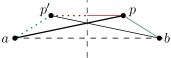
Figure 3: By triangle inequality and symmetry we have $\|pb\|+\|pp^{\prime}\|\geq\|p^{\prime}b\|=\|pa\|$. page

Note that all four trees on the left-hand side include edge $ab$ and since $ab$ is a diameter, we can without loss of generality assume that $T_{\operatorname{cr}}$ contains it too. Thus we can use the notation $\ell_{T}(p)$ as defined above. Assume the following holds for all $p\in\mathcal{P}\setminus\{a,b\}$,

$$\frac{\ell_{S_{a}}(p)+2\ell_{T_{a,b}}(p)+2\ell_{T_{b,a}}(p)+\ell_{S_{b}}(p)}{6}\geq\frac{2}{3}\cdot\ell_{T_{\operatorname{cr}}}(p)\cref@constructprefix{page}{\cref@result}$$ (1)

then summing up over all points $p\in\mathcal{P}\setminus\{a,b\}$ and adding $\|ab\|$ to both sides yields the desired result.

Without loss of generality, suppose that $\|pa\|\geq\|pb\|$ and let $p^{\prime}$ be the reflection of $p$ about the perpendicular bisector of $ab$. Since $\mathcal{P}$ is flat, we have $\ell_{T_{\operatorname{cr}}}(p)\leq\max\{\|pa\|,\|pb\|\}=\|pa\|$. Moreover, $\ell_{T_{b,a}}(p)\geq\|pp^{\prime}\|/2$ and $\ell_{T_{a,b}}(p)=\|pa\|$. Using the triangle inequality in $\triangle bpp^{\prime}$, the left-hand side of (1) is thus at least

$$\frac{\|pa\|+2\|pa\|+\|pp^{\prime}\|+\|pb\|}{6}\geq\frac{\|bp^{\prime}\|+3\|pa\|}{6}=\frac{2}{3}\cdot\|pa\|\geq\frac{2}{3}\cdot\ell_{T_{\operatorname{cr}}}(p)$$

as desired.

Now we use a similar approach to show the main theorem of this section:

See 1.1

Proof 3.5.

We outline the proof strategy, referring to lemmas that will be proved later in this section. Without loss of generality, suppose $\mathcal{P}$ has diameter 2. Consider the longest edge $ab$ of $T_{\scriptscriptstyle\mathrm{OPT}}$ and denote its length by $2d$ (we have $d\leq 1$).

Let $u$ and $v$ be the points realizing the diameter. If $2d\leq 1/f$, then we can show (lem:short) that either $S_{u}$ or $S_{v}$ is long enough. Hence from now on, we can assume that $2df>1$.

Note that $\mathcal{P}$ lies inside the lens $D(a,2)\cap D(b,2)$; the points $a$ and $b$ are in the interior of the lens. Without loss of generality, suppose that $a=(-d,0)$ and $b=(d,0)$. We split the lens into the far region and the truncated lens, as follows and depicted in fig:approx-factor.

Let $s,s^{\prime}$ be the points on the $y$-axis such that $\|sa\|=\|sb\|=\|s^{\prime}a\|=\|s^{\prime}b\|=2df$. We take $s$ to be the one above the $x$-axis. Since $2df>1$, the circles $k=\partial D(s,\|sa\|)$ and $k^{\prime}=\partial D(s^{\prime},\|s^{\prime}a\|)$ intersect the boundary of the lens. The far region then consists of points in the lens above $k$ and of points below $k^{\prime}$. Note that for the points $c$ in the far region the triangle $abc$ is acute-angled and its circumradius $R$ satisfies $R\geq 2df$.

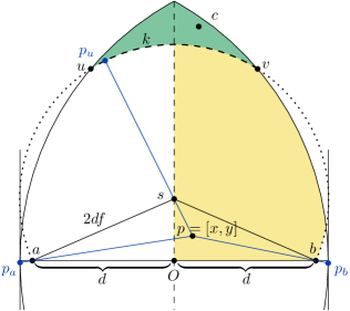
Figure 4: The lens is split into the far region (green) and the truncated lens.page

Next, we argue that if $\mathcal{P}$ contains a point $c$ in the far region, then one of the three stars $S_{a}$, $S_{b}$ or $S_{c}$ is long enough (lem:far). For this, we can restrict our attention to the case when $c$ is above the $x$-axis.

Finally, we argue that if all points of $\mathcal{P}$ lie in the truncated lens, then one of the trees $S_{a}$, $T_{a,b}$, $T_{b,a}$, $S_{b}$ is long enough. Consider those four trees and $T_{\scriptscriptstyle\mathrm{OPT}}$. For these five trees we can again use the notation $\ell_{T}(p)$ as defined above. Given a real parameter $\beta\in(0,1/2)$, define by

$$\operatorname{avg}(p,\beta)=(1/2-\beta)\cdot\ell_{S_{a}}(p)+\beta\cdot\ell_{T_{a,b}}(p)+\beta\cdot\ell_{T_{b,a}}(p)+(1/2-\beta)\cdot\ell_{S_{b}}(p)$$

the weighted average of the lengths of the edges assigned to point $p$, over the four trees $S_{a}$, $T_{a,b}$, $T_{b,a}$, $S_{b}$. We aim to find $\beta\in(0,1/2)$ such that, for each point $p\neq a,b$, we have

$$\cref@constructprefix{page}{\cref@result}\operatorname{avg}(p,\beta)\geq f\cdot\ell_{T_{\scriptscriptstyle\mathrm{OPT}}}(p).$$ (2)

In contrast to the proof to thm:approximation-flat we have to work more to find a suitable $\beta$. Below we will show that $\beta\doteq 0.1604$ works. Summing over $p\in\mathcal{P}\setminus\{a,b\}$ and adding $\|ab\|$ to both sides, we then deduce that

$$(1/2-\beta)\cdot|S_{a}|+\beta\cdot|T_{a,b}|+\beta\cdot|T_{b,a}|+(1/2-\beta)\cdot|S_{b}|\geq f\cdot|T_{\scriptscriptstyle\mathrm{OPT}}|,$$

thus at least one of the four trees $S_{a}$, $T_{a,b}$, $T_{b,a}$, $S_{b}$ has total length at least $f\cdot|T_{\scriptscriptstyle\mathrm{OPT}}|$.

For proving the inequality (2), we can without loss of generality assume that $p=(x,y)$ with $x,y\geq 0$. Let $p_{a}$ be the point with $x$-coordinate $-(2-d)$ on the ray $pa$ and $p_{b}$ be the point with $x$-coordinate $2-d$ on the ray $pb$. When the $x$-coordinate of $p$ is at least $d$, then the ray $pb$ does not intersect the vertical line with $x$-coordinate $2-d$ and we set $p_{b}=b$. Additionally, define $p_{u}$ to be the furthest point from $p$ on the portion of the boundary of the far region that is contained in the circle $k=\partial D(s,2df)$. The proof now proceeds in the following steps.

• We establish the upper bound

  $$\ell_{T_{\scriptscriptstyle\mathrm{OPT}}}(p) \leq\min\bigl{\{}2d,\,\max\{\|pp_{a}\|,\|pp_{b}\|,\|pp_{u}\|\}\bigr{\}} (\text{\cref{lem:topt}})$$

  and thus only have to consider bounds for $\|pp_{a}\|,\|pp_{b}\|$ and $\|pp_{u}\|$.

• We show that the term $\|pp_{b}\|$ in the upper bound on $\ell_{T_{\scriptscriptstyle\mathrm{OPT}}}(p)$ can be ignored (Lemma 3.12).

• We establish a lower bound on $\operatorname{avg}(p,\beta)$ (lem:ab-construction).

• We use the lower bound on $\operatorname{avg}(p,\beta)$ to identify constraints on $\beta$ such that

  $$\operatorname{avg}(p,\beta) \geq f\cdot\min\{2d,\|pp_{a}\|\} (\text{\cref{lem:left}})$$

  $$\operatorname{avg}(p,\beta) \geq f\cdot\min\{2d,\|pp_{u}\|\} (\text{\cref{lem:up}})$$

This reduces the problem to showing that there exists a number $\beta$ that satisfies both the constraints coming from Lemma 3.16 and Lemma 3.18. The most stringent constraints turn out to be those coming from Lemma 3.18, namely:

$$\cref@constructprefix{page}{\cref@result}\frac{2f-1}{2\sqrt{5-8f}-1}\leq\beta\leq 1-f\sqrt{4f^{2}-1}-2f^{2}.$$ (3)

Straightforward algebra (lem:algebra) shows that for our definition of $f$, the left-hand side and the right-hand side of (3) are in fact equal, hence we can set $\beta\doteq 0.1604$ to be their joint value. (The value $f=5/8$ also makes the left and the right sides of (3) equal, but it is not suitable because it gives $\beta<0$.)

To summarize, for the value $f\doteq 0.5467$ defined in the statement of the Theorem, the value $\beta=1-f\sqrt{4f^{2}-1}-2f^{2}\doteq 0.1604$ and for each point $p\neq a,b$, we have

$$\operatorname{avg}(p,\beta) \geq f\cdot\max\bigl{\{}\min\{2d,\|pp_{a}\|\},\,\min\{2d,\|pp_{u}\|\}\bigr{\}}$$

$$\geq f\cdot\min\bigl{\{}2d,\,\max\{\|pp_{a}\|,\|pp_{u}\|\}\bigr{\}}$$

$$\geq f\cdot\ell_{T_{\scriptscriptstyle\mathrm{OPT}}}(p)$$

and the result follows.

It remains to prove Lemmas 3.6 to 3.20. Unfortunately, the statements of those Lemmas rely on the notation already introduced in the proof of thm:approximation. Thus, to follow the rest of this section, one has to understand the concepts and the notation introduced in the proof of thm:approximation.

Lemma 3.6.

page Let $\mathcal{P}$ be a point set and the points $u$ and $v$ realize its diameter. Suppose that $\|uv\|=2$ and that each edge of the optimal tree $T_{\scriptscriptstyle\mathrm{OPT}}$ has length at most $1/f$. Then $\max\{|S_{u}|,|S_{v}|\}\geq f\cdot|T_{\scriptscriptstyle\mathrm{OPT}}|$.

Proof 3.7.

By the triangle inequality, for any point $p\in\mathcal{P}$ we have $\|pu\|+\|pv\|\geq\|uv\|$. Hence

$$|S_{u}|+|S_{v}|=\sum_{p\in\mathcal{P}}\|pu\|+\|pv\|\geq n\cdot\|uv\|=2n,$$

implying that $\max\{|S_{u}|,|S_{v}|\}\geq n$. On the other hand, since each of the $n-1$ edges in $T_{\scriptscriptstyle\mathrm{OPT}}$ has length at most $1/f$, we get

$$f\cdot|T_{\scriptscriptstyle\mathrm{OPT}}|\leq f\cdot(n-1)\cdot\frac{1}{f}\leq n$$

and we are done.

Lemma 3.8.

page Let $ab$ (with $\|ab\|=2d$) be the longest edge of $T_{\scriptscriptstyle\mathrm{OPT}}$. If $\mathcal{P}$ contains a point $c$ in the far region, then $\max\{|S_{a}|,|S_{b}|,|S_{c}|\}\geq f\cdot|T_{\scriptscriptstyle\mathrm{OPT}}|$.

Proof 3.9.

By the definition of the far region, the triangle $abc$ is acute-angled and its circumradius $R$ satisfies $R\geq 2df$. Let $g$ be the center of mass of the pointset $\mathcal{P}_{0}\equiv\mathcal{P}\setminus\{a,b,c\}$. (Such a point set may have points below and above the $x$-axis, but that does not affect the argument.) Then for any point $v$ in the plane we have $\overrightarrow{vg}=\frac{1}{|\mathcal{P}_{0}|}\sum_{p\in\mathcal{P}_{0}}\overrightarrow{vp}$.

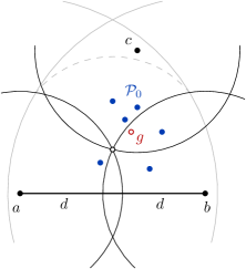
Figure 5: Lemma 3.8. In the illustration, $\mathcal{P}_{0}$ consists of 6 points and we can take $v=a$. The point through three circles is the center of the circle through $a,b,c$.page

Since the triangle $abc$ is acute-angled, there exists a vertex $v\in\{a,b,c\}$ of the triangle such that $\|vg\|\geq R$. Triangle inequality then gives

$$\sum_{p\in\mathcal{P}_{0}}\|vp\|\geq|\mathcal{P}_{0}|\cdot\|vg\|\geq(n-3)\cdot R.$$

Together with $\|va\|+\|vb\|+\|vc\|\geq 2R$ which holds for any acute-angled triangle, this yields

$$|S_{v}|\geq(n-3)R+2R=(n-1)\cdot R\geq(n-1)\cdot 2df\geq f\cdot|T_{\scriptscriptstyle\mathrm{OPT}}|,$$

where in the last inequality we used that each edge of $T_{\scriptscriptstyle\mathrm{OPT}}$ has length at most $2d$.

Recall that $ab$ is the longest edge of $T_{\scriptscriptstyle\mathrm{OPT}}$, that we assumed $a=(-d,0)$, $b=(d,0)$ and that $2df>1$. Note that the point $s$ has coordinates $s=(0,\sqrt{(2df)^{2}-d^{2}})$. We also noted that the two circle $k=D(s,\|sa\|)$ always intersect the lens $D(a,2)\cap D(b,2)$. Consider the two intersection points of $k$ with the boundary of the lens with largest $y$-coordinate and call them $u$ and $v$, where $u$ is to the left of $v$. Refer to fig:approx-factor or fig:topt for an illustration.

For each point $p=(x,y)$ in the truncated lens with $x,y\geq 0$, recall that we have defined the following points:

• $p_{a}$ is the point on the ray $pa$ whose $x$-coordinate equals $-(2-d)$;

• $p_{b}$ is the point on the ray $pb$ whose $x$-coordinate equals $2-d$, if $x(p)<d$, and $p_{b}=b$ if $x(p)\geq d$.

• $p_{u}$ is the the point on the arc of $k$ from $u$ to $v$ that is furthest from $p$. Thus, if the line through $sp$ intersects the arc of $k$ from $u$ to $v$, then $p_{u}$ is that intersection point, otherwise $p_{u}=u$.

Figure 6: For $p\in E$ we have $\ell_{T_{\scriptscriptstyle\mathrm{OPT}}}(p)\leq 2d$, for $p\in N$ we have $\ell_{T_{\scriptscriptstyle\mathrm{OPT}}}(p)\leq\max\{\|pp_{a}\|,\|pu\|\}$ and for $p\in S$ we have $\ell_{T_{\scriptscriptstyle\mathrm{OPT}}}(p)\leq\max\{\|pp_{a}\|,\|pp_{u}\|\}$.page

Lemma 3.10.

page For each point $p=(x,y)$ in the truncated lens with $x,y\geq 0$ we have

$$\ell_{T_{\scriptscriptstyle\mathrm{OPT}}}(p)\leq\min\{2d,\max\{\|pp_{a}\|,\|pp_{b}\|,\|pp_{u}\|\}\}.$$

Proof 3.11.

As $p$ lies in the first quadrant, we only have to consider the truncated lens in this quadrant. Let $l$ and $r$ be the left and right most points of $D(a,2)\cap D(b,2)$. Thus $r=(2-d,0)$ and $l=(d-2,0)$.

For the following we further subdivide the truncated lens into regions; again see fig:topt for an illustration. First of all we denote the region inside the truncated lens but outside of $D(l,2d)$ by $E$. The remainder of the truncated lens we divide into the part $N$ above the line $us$ and the part $S$ below that line.

Note that if $p$ lies in $E$ then $\|pp_{a}\|\geq\|pl\|\geq 2d$, hence the right-hand side equals $2d$. Since the left-hand side is at most $2d$ by assumption, the claim is true.

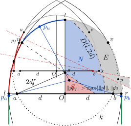
Figure 7: The point $p_{f}$ lies on the arc $ul$. The set of points $p$ such that $\|pp_{f}\|>\max\{\|pl\|,\|pu\|\}$ forms a convex wedge with vertex $b$ fully contained in the fourth quadrant. page

So from now on we can assume that $p\in N\cup S$. This directly implies that $p_{b}\neq b$ and $x(p_{b})=2-d$. Let $p_{f}$ be the point within the truncated lens furthest from $p$. Clearly, $p_{f}$ lies on the boundary of the truncated lens. Since $\ell_{T_{\scriptscriptstyle\mathrm{OPT}}(p)}\leq 2d$ by assumption, it suffices to show that $\|pp_{f}\|\leq\max\{\|pp_{a}\|,\|pp_{b}\|,\|pp_{u}\|\}$. Let $t$ be the top-most point of the truncated lens. We distinguish 5 cases:

1. $p_{f}$ lies in the third quadrant: Then $\|pp_{f}\|\leq\|pp_{a}\|$.

2. $p_{f}$ lies in the fourth quadrant: Then $\|pp_{f}\|\leq\|pp_{b}\|$.

3. $p_{f}$ lies in the first quadrant: Consider the reflection $p_{f}^{\prime}$ of $p_{f}$ about the $y$-axis. Since $x\geq 0$ we have $\|pp_{f}^{\prime}\|\geq\|pp_{f}\|$, and the inequality is strict when $x>0$. Thus, when $x>0$, this case cannot occur, and when $x=0$, it reduces to the case where $p_{f}$ belongs to the second quadrant.

4. $p_{f}$ lies in the second quadrant:

   1. $p_{f}$ lies on the arc $tu$ (fig:topt): If $p$ lies in $N$ then for any $q$ on the arc $tu$ we have $\|pq\|\leq\|pu\|=\|pp_{u}\|$, thus also $\|pp_{f}\|\leq\|pp_{u}\|$. If $p$ lies in $S$ then, by triangle inequality, $\|pp_{f}\|\leq\|ps\|+\|sp_{f}\|=\|ps\|+2df=\|pp_{u}\|$.

   2. page $p_{f}$ lies on the arc $ul$: We claim that $\|pp_{f}\|\leq\max\{\|pl\|,\|pu\|\}$. Indeed, the perpendicular bisectors of segments $p_{f}l$ and $p_{f}u$ intersect at $b$ and thus the points for which the claim fails all lie in a convex wedge with vertex $b$ that is fully contained in the fourth quadrant, see fig:topt_case5. Since $\|pl\|\leq\|pp_{a}\|$ and $\|pu\|\leq\|pp_{u}\|$, we get $\|pp_{f}\|\leq\max\{\|pp_{a}\|,\|pp_{u}\|\}$.

Lemma 3.12.

page Let $p=(x,y)$ be any point in the truncated lens with $x,y\geq 0$. If $\|pp_{a}\|\leq 2d$, then $\|pp_{b}\|\leq\|pp_{a}\|$.

Proof 3.13.

We present a straightforward algebraic proof (we are not aware of a purely geometric proof). The case $x=0$ is clear because of symmetry; in that case $\|pp_{b}\|=\|pp_{a}\|$. Thus, we only consider the case $x>0$. Since $\|pp_{a}\|\leq 2d$, we must have $x<d$, and therefore $p_{b}$ has $x$-coordinate $2-d$ (and $p_{b}\neq b$).

Figure 8: The situation for lem:right.

From similar triangles and a Pythagorean theorem we have $\|pp_{a}\|=\|pa\|\cdot\frac{2-d+x}{d+x}$ and $\|pa\|^{2}=(d+x)^{2}+y^{2}$. Therefore the assumption $\|pp_{a}\|^{2}\leq(2d)^{2}$ can be equivalently rewritten as

$$\cref@constructprefix{page}{\cref@result}(y^{2}+(d+x)^{2})\cdot\frac{(2-d+x)^{2}}{(d+x)^{2}} \leq 4d^{2}$$

$$y^{2} \leq\frac{(4d^{2}-(2-d+x)^{2})(d+x)^{2}}{(2-d+x)^{2}}.$$ (4)

Similarly as with $\|pp_{a}\|^{2}$, we express $\|pp_{b}\|^{2}$ as

$$\|pp_{b}\|^{2}=(y^{2}+(d-x)^{2})\cdot\frac{(2-d-x)^{2}}{(d+x)^{2}}$$ (5)

and rewrite our goal $\|pp_{b}\|^{2}\leq\|pp_{a}\|^{2}$ as

$$(y^{2}+(d-x)^{2})\cdot\frac{(2-d-x)^{2}}{(d-x)^{2}} \leq(y^{2}+(d+x)^{2})\cdot\frac{(2-d+x)^{2}}{(d+x)^{2}}$$

$$y^{2}\cdot\frac{(2-d-x)^{2}(d+x)^{2}-(2-d+x)^{2}(d-x)^{2}}{(d+x)^{2}(d-x)^{2}} \leq(2-d+x)^{2}-(2-d-x)^{2},$$

which, upon expanding the parentheses and dividing by $4x>0$ transforms into the goal

$$y^{2}\cdot\frac{2(1-d)(2d-d^{2}-x^{2})}{(d+x)^{2}(d-x)^{2}}\leq 2-d.$$

We plug in the upper bound on $y^{2}$ from (3.13), cancel the term $(d+x)^{2}$, and clear the denominators. This leaves us with proving

$$(4d^{2}-(2-d+x)^{2})\cdot 2(1-d)(2d-d^{2}-x^{2})\leq(2-d+x)^{2}\cdot(2-d)(d-x)^{2}$$

which, upon expanding the parentheses, reduces to

$$\cref@constructprefix{page}{\cref@result}0\leq(16d-32d^{2}+8d^{3}+16d^{4}-7d^{5})+x^{2}(-8d+16d^{2}-10d^{3})+dx^{4}.$$ (6)

For any fixed $d>0$, the right-hand side $Q(d,x^{2})$ is a quadratic function of $x^{2}$ with positive coefficient $d>0$ by the leading term $(x^{2})^{2}$, hence the minimum of $Q(d,x^{2})$ is attained when

$$x^{2}=\frac{8d-16d^{2}+10d^{3}}{2d}=4-8d+5d^{2}.$$

Plugging $x^{2}=4-8d+5d^{2}$ into (6) and expanding the parentheses for the last one time we are left to prove

$$0 \leq 32d^{2}-96d^{3}+96d^{4}-32d^{5}$$

$$0 \leq 32d^{2}(1-d)^{3}$$

which is true since $d\leq 1$.

Lemma 3.14.

page Let $p=(x,y)$ be any point in the plane with $x,y\geq 0$ and let $\beta\in(0,1/2)$ be a real number. Then

$$\operatorname{avg}(p,\beta)\geq\frac{d\cdot(1-\beta)+x\cdot 2\beta}{d+x}\cdot\|pa\|.$$

Proof 3.15.

Unpacking the definition we have

$$\operatorname{avg}(p,\beta)\geq(1/2-\beta)\cdot\|pa\|+\beta\cdot\|pa\|+\beta\cdot x+(1/2-\beta)\cdot\|pb\|.$$

Figure 9: Mirroring $p$ along the $y$-axis in lem:ab-construction. page

Let $p^{\prime}=(-x,y)$ be the reflection of $p$ about the $y$ axis (see fig:ab). The triangle inequality $\|p^{\prime}p\|+\|pb\|\geq\|p^{\prime}b\|=\|pa\|$ leads to $\beta\cdot x=\frac{1}{2}\beta\cdot\|p^{\prime}p\|\geq\frac{1}{2}\beta\cdot(\|pa\|-\|pb\|)$, and we obtain

$$\operatorname{avg}(p,\beta)\geq\frac{1}{2}\cdot\|pa\|+\frac{1}{2}\beta\cdot\|pa\|+\left(\frac{1}{2}-\frac{3}{2}\beta\right)\cdot\|pb\|.$$

Next we claim that $\|pb\|\geq\frac{d-x}{d+x}\cdot\|pa\|$: Indeed, upon squaring, using the Pythagorean theorem and clearing the denominators this becomes $y^{2}\cdot 4dx\geq 0$ which is true. Using this bound on the term containing $\|pb\|$ we finally get the desired

$$\operatorname{avg}(p,\beta)\geq\frac{(1+\beta)(d+x)+(1-3\beta)(d-x)}{2(d+x)}\cdot\|pa\|=\frac{(1-\beta)\cdot d+2\beta\cdot x}{d+x}\cdot\|pa\|.$$

Lemma 3.16.

page Let $p=(x,y)$ be any point in the lens with $x,y\geq 0$. Suppose

$$\frac{2f-1}{5-8f}\leq\beta\leq\frac{1}{2}\cdot f.$$

Then $\operatorname{avg}(p,\beta)\geq f\cdot\min\{2d,\|pp_{a}\|\}$.

Proof 3.17.

It suffices to show that:

1. If $x\geq 3d-2$, then $\operatorname{avg}(p,\beta)\geq f\cdot 2d$.

2. If $x\leq 3d-2$, then $\operatorname{avg}(p,\beta)\geq f\cdot\|pp_{a}\|$.

We consider those two cases independently.

1. page Using Lemma 3.14 and the inequalities $\|pa\|\geq d+x$ and $x\geq 3d-2$, we rewrite

   $$\operatorname{avg}(p,\beta)\geq\frac{d\cdot(1-\beta)+x\cdot 2\beta}{d+x}\cdot\|pa\|\geq d-d\beta+(3d-2)\cdot 2\beta=\beta(5d-4)+d.$$

   Hence it suffices to prove $\beta\cdot(5d-4)\geq d(2f-1)$. Using the lower bound on $\beta$ and $4\leq 8df$ we get

   $$\beta\cdot(5d-4)\geq\beta\cdot(5d-8df)\geq\frac{2f-1}{5-8f}\cdot d\cdot(5-8f)=d(2f-1)$$

   as desired. Note that $2f-1$ and $5-8f$ are both positive.

2. We have $\|pp_{a}\|=\|pa\|\cdot\frac{2-d+x}{d+x}$. Using Lemma 3.14 it suffices to prove

   $$d(1-\beta)+x\cdot 2\beta \geq f(2-d+x)$$

   $$d(1-\beta)-f(2-d) \geq x(f-2\beta).$$

   Since $f\geq 2\beta$ by assumption, the right-hand side is increasing in $x$ and we can plug in $3d-2$ for $x$. This leaves us with proving the inequality

   $$d(1-\beta)-f(2-d) \geq(3d-2)(f-2\beta)$$

   $$\beta\cdot(5d-4) \geq d(2f-1),$$

   which is the same inequality as in the first case.

Lemma 3.18.

page Let $p=(x,y)$ be any point in the lens with $x,y\geq 0$. Suppose that $\beta<\frac{151}{304}\cdot f$, that $\frac{1}{2}\leq f\leq\frac{19}{32}$ and that

$$\frac{2f-1}{2\sqrt{5-8f}-1}\leq\beta\leq 1-f\sqrt{4f^{2}-1}-2f^{2}.$$

Then

$$\operatorname{avg}(p,\beta)\geq f\cdot\min\{2d,\|pp_{u}\|\}.\cref@constructprefix{page}{\cref@result}$$

Proof 3.19.

Because of the lower bound for $\operatorname{avg}(p,\beta)$ in lem:ab-construction, to show the statement it suffices to show that

$$\frac{d\cdot(1-\beta)+x\cdot 2\beta}{d+x}\cdot\|pa\|\geq f\cdot\min\{2d,\|pp_{u}\|\}.\cref@constructprefix{page}{\cref@result}$$ (7)

We will consider the two cases $y\leq y(u)$ and $y>y(u)$ separately.

Case 1: $y\leq y(u)$

Define $\lambda=\frac{d\cdot(1-\beta)+x\cdot 2\beta}{d+x}\cdot\|pa\|$. We have to show that $\lambda\geq f\cdot\min\{2d,\|pp_{u}\|\}$. Note that $\lambda$ is an increasing function of $y$ because $\|pa\|$ is also increasing with $y$. On the other hand, $\|pp_{u}\|$ is a decreasing function of $y$ for $y\leq y(u)$: If $p_{u}\neq u$, then $\|pp_{u}\|=\|ps\|+2df$ is decreasing in $y$, and if $p_{u}=u$ then $\|pp_{u}\|=\|pu\|$ decreases when $y$ increases (for $y\leq y(u)$). It follows that $\min\{2d,\|pp_{u}\|\}$ is a decreasing function of $y$ for $y\leq y(u)$.

As $\min\{2d,\|pp_{u}\|\}$ is decreasing and $\lambda$ is increasing in $y$, for $y\leq y(u)$, to handle our current case it suffices to show (7) for $y=0$. Now we have $\|pa\|=d+x$, so we can rewrite $\lambda$ as $\lambda_{0}=d\cdot(1-\beta)+x\cdot 2\beta$, which is positive.

Let $q=(q_{x},0),q_{x}\geq 0$ be the point on the $x$-axis such that $\|qs\|=2d(1-f)$. This means that for $p=q$ we have $\|pp_{u}\|\leq\|ps\|+\|sp_{u}\|=2d$ (see Figure 10). We further split between cases depending on whether $0\leq x\leq q_{x}$ or $x>q_{x}$.

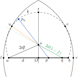
Figure 10: Lemma 3.18. page

Case 1a:

$0\leq x\leq q_{x}$. We will show that in this case $\lambda_{0}\geq f\cdot\|pp_{u}\|$. The Pythagorean theorem gives

$$f\cdot\|pp_{u}\|\leq f\cdot\|ps\|+f\cdot\|sp_{u}\|=f\sqrt{x^{2}+(2df)^{2}-d^{2}}+2df^{2}$$

Therefore, substituting $\lambda_{0}$, it suffices to show

$$d\cdot(1-\beta)+x\cdot 2\beta \geq f\sqrt{x^{2}+(2df)^{2}-d^{2}}+2df^{2}.\cref@constructprefix{page}{\cref@result}$$ (8)

When $\beta<\frac{151}{304}\cdot f$ and $f\leq\frac{19}{32}$, the term $d\cdot(1-\beta)-2df^{2}$ is positive and the last inequality is equivalent to

$$0 \geq f^{2}\cdot(x^{2}+(2df)^{2}-d^{2})-(d\cdot(1-\beta)+x\cdot 2\beta-2df^{2})^{2}$$

The right-hand side is a quadratic function of $x$ with positive coefficient $f^{2}-4\beta^{2}$ by the leading term, hence it suffices to check the inequality (8) for $x\in\{0,q_{x}\}$.

For $x=0$, we need to check that $d(1-\beta)\geq f(\sqrt{d^{2}(4f^{2}-1)}+2df)$, which reduces precisely to the assumption

$$\beta\leq 1-f\sqrt{4f^{2}-1}-2f^{2}.$$

For $x=q_{x}$, the Pythagorean theorem gives $(q_{x})^{2}=(2d(1-f))^{2}+d^{2}-(2df)^{2}=d^{2}\cdot(5-8f)$, hence $q_{x}=d\sqrt{5-8f}$. The point $q$ has been selected so that $\|ps\|+\|sp_{u}\|=2d$, and therefore the right side of (8) is $2df$. We thus have to verify that

$$d(1-\beta)+d\sqrt{5-8f}\cdot 2\beta \geq f\cdot 2d\cref@constructprefix{page}{\cref@result}$$ (9)

$$\beta\cdot(2\sqrt{5-8f}-1) \geq 2f-1.$$

Since $f\leq 19/32$, the term in the parentheses on the left-hand side is positive, and after dividing we obtain precisely the assumption.

Case 1b:

$q_{x}<x$. In this case we show that $\lambda_{0}\geq f\cdot 2d$. Since the term $\lambda_{0}$ is increasing in $x$ and $2d$ is constant, we only need to show that $\lambda_{0}\geq f\cdot 2d$ for $x=q_{x}$. However, this was already shown in the previous case; see (9).

Case 2: $y>y(p_{u})$

In this case we have $\|pp_{u}\|=\|pu\|\leq\|uv\|$. Furthermore, because $4df>2d$, the intersection of the line supporting $bs$ with the circle $k$ is outside the lens. That intersection point has $x$-coordinate $-d$ because of symmetry with respect to $s$, and since $u$ is above it, we have $x(u)\geq-d$ as well as $x\leq d$. So we have $\min\{2d,\|pp_{u}\|\}=\|pp_{u}\|$. This means that to show (7) we have to show

$$\frac{d(1-\beta)+2x\beta}{d+x}\cdot\|pa\| \geq f\cdot\|pp_{u}\|.$$

As $p$ lies above the horizontal line through $u$, we get $\|pa\|\geq\|pp_{u}\|$, thus it suffices to show

$$\frac{d(1-\beta)+2x\beta}{d+x} \geq f$$

$$d-d\beta+2x\beta \geq fd+fx$$

$$d(1-(\beta+f)) \geq x(f-2\beta)$$

$$x \leq d\cdot\frac{1-(\beta+f)}{f-2\beta}$$

As we know $x\leq d$ this is true for

$$\frac{1-(\beta+f)}{f-2\beta} \geq 1$$

$$1-(\beta+f) \geq f-2\beta$$

$$\beta \geq 2f-1,$$

where in the last step we used that $f>2\beta$. The last condition is a looser bound than the left side of the statement of the lemma as $f\geq\frac{1}{2}$ and therefore $2\cdot\sqrt{5-8f}-1\leq 1$.

Lemma 3.20.

page The positive solutions of

$$\frac{2x-1}{2\sqrt{5-8x}-1}=1-x\sqrt{4x^{2}-1}-2x^{2}$$

are $x=\tfrac{5}{8}$ and the fourth smallest root of

$$-80+128x+504x^{2}-768x^{3}-845x^{4}+1096x^{5}+256x^{6}.$$

Proof 3.21.

We provide a sketch of how to solve it “by hand”. One can also use advanced software for algebraic manipulation. Setting the polynomials $q_{1}(x)=4x^{2}-1$ and $q_{2}(x)=5-8x$, and multiplying both sides of the equation by the denominator on the left-hand side, we are left with the equation

$$2x-2x^{2} =x\sqrt{q_{1}(x)}-(2-4x^{2})\sqrt{q_{2}(x)}-2x\sqrt{q_{1}(x)q_{2}(x)}$$

$$2x-2x^{2}+2x\sqrt{q_{1}(x)q_{2}(x)} =x\sqrt{q_{1}(x)}-(2-4x^{2})\sqrt{q_{2}(x)}.$$

Squaring both sides, which may introduce additional roots, we get, for some polynomials $q_{3}(\,),\dots,q_{6}(\,)$, the equation

$$q_{3}(x)+q_{4}(x)\sqrt{q_{1}(x)q_{2}(x)} =q_{5}(x)+q_{6}(x)\sqrt{q_{1}(x)q_{2}(x)}$$

$$q_{3}(x)-q_{5}(x) =\bigl{(}q_{6}(x)-q_{4}(x)\bigr{)}\sqrt{q_{1}(x)q_{2}(x)}.$$

Squaring both sides gain, which may introduce additional solutions, we get the polynomial

$$8(x-\tfrac{5}{8})(-80+128x+504x^{2}-768x^{3}-845x^{4}+1096x^{5}+256x^{6})=0$$

This polynomial has 7 real roots that can be approximated numerically. The smallest three roots of this polynomial are negative ($x\doteq-4.82037$, $x\doteq-0.657898$ and $x\doteq-0.523446$). The fourth smallest root, $x\doteq 0.546723$, is a solution to the original equation. The fifth and sixth roots are $x\doteq 0.577526$ and $x\doteq 0.596211$, which are not solutions to the original equation. The largest root of the polynomial is $x=\tfrac{5}{8}$, which is also a solution to the original equation.

4 Convex and flat convex point sets

page

In this section we present two results for convex point sets. First, we show that if $\mathcal{P}$ is a convex point set then the longest plane tree is a caterpillar (see thm:convex) and that any caterpillar could be the unique longest plane tree (see thm:caterpillars). Second, by looking at suitable flat convex sets we prove upper bounds on the approximation factor $\operatorname{BoundDiam}(d)$ achieved by the longest plane tree among those with diameter at most $d$.

4.1 Convex sets and caterpillars

page

We say that a tree $C$ is a caterpillar if it contains a path $P$ such that each node $v\in C$ not lying on $P$ is adjacent to a node on $P$. Equivalently, a tree is a caterpillar if its edges can be listed in such an order that every two consecutive edges in the list share an endpoint.

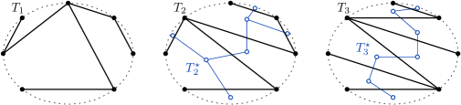
Figure 11: Left: A tree $T_{1}$ that spans $\mathcal{P}$ but it is not a caterpillar. Middle: A tree $T_{2}$ that is a caterpillar but it is not zigzagging. Right: A tree $T_{3}$ that is a zigzagging caterpillar – the dual tree $T_{3}^{\star}$ is a path. page

Throughout this section we consider trees that span a given convex point set $\mathcal{P}$. We say that (a drawing of) such a tree $T$ is a zigzagging caterpillar if $T$ is a caterpillar and the dual graph $T^{\star}$ of $T$ is a path. Here a dual graph $T^{\star}$ is defined as follows: Let $C$ be a smooth closed curve passing through all points of $\mathcal{P}$. The curve bounds a convex region and the $n-1$ edges of $T$ split that region into $n$ subregions. The graph $T^{\star}$ has a node for each such subregion and two nodes are connected if their subregions share an edge of $T$ (see fig:zigzag).

First we prove that the longest plane tree of any convex set is a zigzagging caterpillar. See 1.2

Proof 4.1.

Let $T_{\scriptscriptstyle\mathrm{OPT}}$ be a longest plane tree. We prove that $T_{\scriptscriptstyle\mathrm{OPT}}^{\star}$ is a path by contradiction.

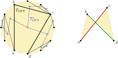
Figure 12: Left: A convex point set with a (fake) longest plane tree $T_{\scriptscriptstyle\mathrm{OPT}}$ (black) and the dual graph $T_{\scriptscriptstyle\mathrm{OPT}}^{\star}$ (blue). Right: If $T_{\scriptscriptstyle\mathrm{OPT}}^{\star}$ has a node of degree 3 or more, a longer tree can be constructed by replacing one dotted edge of $T_{\scriptscriptstyle\mathrm{OPT}}$ by a longer edge (of the same color). page

Suppose a node $v$ of $T_{\scriptscriptstyle\mathrm{OPT}}^{\star}$ has degree at least 3 and let $ab$, $bc$, $cd$ be three corresponding edges of $T_{\scriptscriptstyle\mathrm{OPT}}$ (see fig:convex). Since the quadrilateral $abcd$ is convex, by triangle inequality we have $\|ab\|+\|cd\|<\|ac\|+\|bd\|$. Hence either $\|ab\|<\|ac\|$ or $\|cd\|<\|bd\|$ (or both). Since $T_{1}=T_{\scriptscriptstyle\mathrm{OPT}}\cup\{ac\}\setminus\{ab\}$ and $T_{2}=T_{\scriptscriptstyle\mathrm{OPT}}\cup\{bd\}\setminus\{cd\}$ are both plane trees, at least one of them is longer than $T_{\scriptscriptstyle\mathrm{OPT}}$, a contradiction.

Conversely, for each caterpillar $C$ we will construct a convex set $\mathcal{P}_{C}$ whose longest plane tree is isomorphic to $C$. In fact, $\mathcal{P}_{C}$ will be not only convex but also a “flat arc”. Formally, we say that a set $\mathcal{P}$ of $n=m+1$ points $a_{i}=(x_{i},y_{i})$ satisfying $x_{1}<\dots<x_{m+1}$ is a flat arc if it is flat (that is, the absolute values of all $y$-coordinates are negligible) and the points $a_{1},\dots,a_{m+1}$ all lie on the convex hull of $\mathcal{P}$ in this order.

We call the sequence $G(\mathcal{P})=\{g_{i}\}_{i=1}^{m}=\{|x_{i+1}-x_{i}|\}_{i=1}^{m}$ the (horizontal) gap sequence. Lastly, given a tree $T$ spanning a flat arc $\mathcal{P}$, we define its cover sequence $\operatorname{Cov}(T)=\{c_{i}\}_{i=1}^{m}$ to be a list storing the number of times each gap is “covered”. Formally, $c_{i}$ is the number of edges of $T$ that contain a point whose $x$-coordinate lies within the open interval $(x_{i},x_{i+1})$, see fig:flat-convex-2. Note that the gap sequence and the cover sequence determine the length of the tree because $|T|=\sum_{i=1}^{m}c_{i}\cdot g_{i}$.

Figure 13: Given a flat arc $\mathcal{P}$ of $n=m+1$ points, we denote by $G(\mathcal{P})=\{g_{i}\}_{i=1}^{m}$ its gap sequence. Given a tree $T$ spanning $\mathcal{P}$, we denote by $\operatorname{Cov}(T)=\{c_{i}\}_{i=1}^{m}$ its cover sequence. Later we show that the longest plane tree $T_{\scriptscriptstyle\mathrm{OPT}}$ of a flat arc $\mathcal{P}$ is a zigzagging caterpillar containing the edge $a_{1}a_{m+1}$ and that its cover sequence $\operatorname{Cov}(T_{\scriptscriptstyle\mathrm{OPT}})$ is a unimodal (single-peaked) permutation of $\{1,2,\dots,m\}$.page

Before we prove that any caterpillar can be the longest tree of a flat arc, we first show that the cover sequences of zigzagging caterpillars are unimodal (single-peaked) permutations.

Lemma 4.2.

page Consider a flat arc $\mathcal{P}=\{a_{1},\dots,a_{m+1}\}$ and a zigzagging caterpillar $T$ containing the edge $a_{1}a_{m+1}$. Then the cover sequence $\operatorname{Cov}(T)$ of $T$ is a unimodal permutation of $\{1,2,\dots,m\}$.

Proof 4.3.

By induction on $m$. The case $m=1$ is clear.

Fix $m\geq 2$. By the definition of a zigzagging caterpillar, the dual graph $T^{\star}$ of $T$ is a path. Since $a_{1}a_{m+1}$ is an edge of $T$, either $a_{1}a_{m}$ or $a_{2}a_{m-1}$ is an edge of $T$ too. Without loss of generality assume $a_{1}a_{m}$ is an edge of $T$. Then $T\setminus\{a_{1}a_{m+1}\}$ is a zigzagging caterpillar on $m$ points $a_{1},\dots,a_{m}$ containing the edge $a_{1}a_{m}$, hence by induction its cover sequence is a unimodal permutation of $\{1,2,\dots,m-1\}$. Adding the omitted edge $a_{1}a_{m+1}$ adds 1 to each of the $m-1$ elements and appends a 1 to the list, giving rise to a unimodal permutation of $\{1,2,\dots,m\}$. This completes the proof.

Now we are ready to prove that any caterpillar, including a path, can be the longest plane tree of some flat arc. See 1.3

Proof 4.4.

We will define a flat arc $\mathcal{P}_{C}$ such that the unique longest tree $T_{\scriptscriptstyle\mathrm{OPT}}$ of $\mathcal{P}_{C}$ is isomorphic to $C$. Consider a flat arc $\mathcal{P}=\{a_{1},\dots,a_{m+1}\}$, with a yet unspecified gap sequence $\{g_{i}\}_{i=1}^{m}$. Take the caterpillar $C$ and let $T$ be its drawing onto $\mathcal{P}$ that contains the edge $a_{1}a_{m+1}$ and is zigzagging (it is easy to see that such a drawing always exists). By lem:unimodal its cover sequence $\operatorname{Cov}(T)=\{c_{i}\}_{i=1}^{m}$ is a unimodal permutation of $\{1,2,\dots,m\}$. The total length $|T|$ of $T$ can be expressed as $|T|=\sum_{i=1}^{m}c_{i}\cdot g_{i}$.

Now we specify the gap sequence: For $i=1,\dots,m$ set $g_{i}=c_{i}$. It is easy to see that this sequence defines a plane tree $T$; see fig:flat-convex-2. It suffices to show that $T$ coincides with the longest plane tree $T_{\scriptscriptstyle\mathrm{OPT}}$ of $\mathcal{P}$.

By thm:convex, $T_{\scriptscriptstyle\mathrm{OPT}}$ must be a zigzagging caterpillar. Moreover, note that $a_{1}a_{m+1}$ is an edge of $T_{\scriptscriptstyle\mathrm{OPT}}$: Indeed, assume otherwise. Since $a_{1}a_{m+1}$ does not cross any other edge, adding it to $T_{\scriptscriptstyle\mathrm{OPT}}$ produces a plane graph with a single cycle. Since all edges of $T_{\scriptscriptstyle\mathrm{OPT}}$ are shorter than $a_{1}a_{m+1}$, omitting any other edge from that cycle creates a longer plane tree, a contradiction.

Thus we can apply lem:unimodal to $T_{\scriptscriptstyle\mathrm{OPT}}$ and learn that the cover sequence of $T_{\scriptscriptstyle\mathrm{OPT}}$ is some unimodal permutation $\pi$ of $\{1,2,\dots,m\}$ and that its total length $|T_{\scriptscriptstyle\mathrm{OPT}}|$ can be written as $|T_{\scriptscriptstyle\mathrm{OPT}}|=\sum_{i=1}^{m}\pi_{i}\cdot g_{i}$. Since $c_{i}$ and $g_{i}$ match, by rearrangement inequality we have

$$|T_{\scriptscriptstyle\mathrm{OPT}}|=\sum_{i=1}^{m}\pi_{i}\cdot g_{i}\leq\sum_{i=1}^{m}c_{i}\cdot g_{i}=|T|\leavevmode\nobreak\ \leavevmode\nobreak\ \leavevmode\nobreak\ \text{with equality only if $\pi_{i}=c_{i}$ for each $i$.}\cref@constructprefix{page}{\cref@result}$$ (10)

Therefore $T_{\scriptscriptstyle\mathrm{OPT}}=T$ and we are done.

4.2 Upper bounds on $\operatorname{BoundDiam}(d)$bd(d)

The algorithms for approximating $|T_{\scriptscriptstyle\mathrm{OPT}}|$ often produce trees with small diameter. Given an integer $d\geq 2$ and a point set $\mathcal{P}$, let $T^{d}_{\scriptscriptstyle\mathrm{OPT}}(\mathcal{P})$ be a longest plane tree spanning $\mathcal{P}$ among those whose diameter is at most $d$. One can then ask what is the approximation ratio

$$\operatorname{BoundDiam}(d)=\inf_{\mathcal{P}}\frac{|T^{d}_{\scriptscriptstyle\mathrm{OPT}}(\mathcal{P})|}{|T_{\scriptscriptstyle\mathrm{OPT}}(\mathcal{P})|}$$

achieved by such a tree. As before, we drop the dependency on $\mathcal{P}$ in the notation and just use $T^{d}_{\scriptscriptstyle\mathrm{OPT}}$ and $T_{\scriptscriptstyle\mathrm{OPT}}$.

When $d=2$, this reduces to asking about the performance of stars. A result due to Alon, Rajagopalan and Suri [1, Theorem 4.1] can be restated as $\operatorname{BoundDiam}(2)=1/2$. Below we show a crude upper bound on $\operatorname{BoundDiam}(d)$ for general $d$ and then a specific upper bound tailored to the case $d=3$. Note that thm:dp shows that $|T^{3}_{\scriptscriptstyle\mathrm{OPT}}|$ can be computed in polynomial time. Our proofs in this section use the notions of flat arc, gap sequence and cover sequence defined in sec:convex.

See 1.4

Proof 4.5.

Consider a flat arc on $d+2$ points with gap sequence $G=(1,3,5,\dots,d+1,\dots,6,4,2)$. Since $G$ is unimodal, arguing as in the proof of thm:caterpillars we obtain that $T_{\scriptscriptstyle\mathrm{OPT}}$ is the zigzagging caterpillar whose cover sequence is the same unimodal permutation, i.e. a path consisting of $d+1$ edges (and diameter $d+1$). Moreover, this path is the only optimal plane tree spanning the flat arc because of thm:convex and the rearrangement inequality; see the argument leading to (10) in the proof of thm:caterpillars. Therefore, for any other plane spanning tree $T\neq T_{\scriptscriptstyle\mathrm{OPT}}$, be it a zigzagging caterpillar or not, must have a length that is an integer less than $|T_{\scriptscriptstyle\mathrm{OPT}}|$. Using that $|T_{\scriptscriptstyle\mathrm{OPT}}|=\sum_{i=1}^{d+1}i^{2}=\frac{1}{6}(d+1)(d+2)(2d+3)=\frac{1}{3}d^{3}+o(d^{3})$ we obtain

$$\operatorname{BoundDiam}(d)\leq\frac{|T_{\scriptscriptstyle\mathrm{OPT}}|-1}{|T_{\scriptscriptstyle\mathrm{OPT}}|}=1-\frac{6}{(d+1)(d+2)(2d+3)}.$$

When $d=3$, thm:diameter-bound gives $\operatorname{BoundDiam}(3)\leq 29/30$. By tailoring the point set size, the gap sequence $\{g_{i}\}_{i=1}^{m}$, and by considering flat convex sets that are not arcs we improve the bound to $\operatorname{BoundDiam}(3)\leq 5/6$.

See 1.5

Proof 4.6.

Consider a flat point set $\mathcal{P}_{4k+2}$ consisting of two flat arcs symmetric with respect to a horizontal line, each with a gap sequence

$$(\underbrace{1,\dots,1}_{k\times},\ 2k+1,\ \underbrace{1,\dots,1}_{k\times}).$$

In other words, $\mathcal{P}_{4k+2}$ consists of two diametrically opposite points, four unit-spaced arcs of $k$ points each, and a large gap of length $2k+1$ in the middle (see fig:diameter-3).

Figure 14: An illustration of the point set $\mathcal{P}_{4k+2}$ when $k=3$ with a tree $T_{L}$ (red).page

On one hand, straightforward counting gives $|T_{\scriptscriptstyle\mathrm{OPT}}|\geq|T_{L}|=12k^{2}+6k+1$, where $T_{L}$ is the tree depicted in fig:diameter-3. On the other hand, we claim that any tree $T$ with diameter at most $3$ has length at most $10k^{2}+6k+1$. Thus

$$\operatorname{BoundDiam}(3)\leq\frac{10k^{2}+6k+1}{12k^{2}+6k+1},$$

which tends to $5/6$ as $k\to\infty$.

In the rest of this proof we will show that the longest tree $T$ among those with diameter at most $3$ on $\mathcal{P}_{4k+2}$ has length at most $10k^{2}+6k+1$. First, note that as $T$ has diameter at most $3$ it is either a star or it has a cut edge $ab$ whose removal decomposes $T$ into a star rooted at $a$ and a star rooted at $b$.

To add the lengths of the edges of the tree, we will often split the edges across the large gap into two parts: one part contained within the left or the right part and with maximum length $k$, and one part going across the large gap, with a length between $2k+1$ and $2k+1+k=3k+1$.

If $T$ is a star, then without loss of generality we can assume that its root $a$ is to the left of the large gap. Denote the distance from the large gap to $a$ by $i$ (we have $0\leq i\leq k$). Straightforward algebra (see fig:flatstar) then gives

$$|S_{a}| =(k-i)^{2}+i(i+1)\ +\ (2k+1)\cdot(i+2k+1)\ +\ k^{2}$$

$$\leq k(k+1)\ +\ (2k+1)(3k+1)\ +\ k^{2}$$

$$=8k^{2}+6k+1.$$

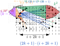
Figure 15: The longest star for $\mathcal{P}_{4k+2}$ is short. page

Now suppose $T$ has diameter $3$ and denote its cut edge by $ab$. If $ab$ is vertical then $|T|=|S_{a}|$ and the above bound applies. In the remaining cases, without loss of generality we can assume that $a$ is to the left of $b$. The line $ab$ then splits the remaining points of $\mathcal{P}_{4k+2}$ into two arcs – one above $ab$ and the other one below it.

We claim that in the longest tree with diameter $3$, the points of one arc are either all connected to $a$ or all to $b$: For the sake of contradiction, fix an arc and suppose $c$ is the rightmost point connected to $a$. Then by the choice of $c$ everything right of it is connected to $b$ and by convexity everything to the left of $c$ is connected to $a$. Let $\ell$ be the vertical line through the midpoint of $ab$. If $c$ lies to the left of $\ell$, moving $c$ to the left increases the length of the tree as the distance to $b$ for all points left of $\ell$ is larger than the distance to $a$. Otherwise, moving it to the right increases the length of the tree. Thus we either have $c=a$ or $c=b$ as claimed.

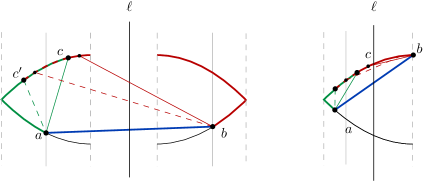
Figure 16: Points on one side of $ab$ are either all connected to $a$ or all to $b$. page

Since $\mathcal{P}_{4k+2}$ is centrally symmetric and we have already dealt with the case when $T$ is a star, we can without loss of generality assume that all points above $ab$ are connected to $a$ and all points below $ab$ are connected to $b$. Now suppose that $a$ is below the diameter line $\ell^{\prime}$ of $\mathcal{P}_{4k+2}$ and consider the reflection $a^{\prime}\in\mathcal{P}_{4k+2}$ of $a$ about $\ell^{\prime}$. Then the tree $T^{\prime}$ with cut edge $a^{\prime}b$ is longer than $T$, since in $T^{\prime}$ the points to the left of $aa^{\prime}$ are connected to $b$ rather than to $a$ and all the other edges have the same length (see fig:diam3bound:first). Hence we can assume that $a$ lies above $\ell^{\prime}$ (or on it). Similarly, $b$ lies below $\ell^{\prime}$ or on it.

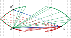
Figure 17: Flipping $a$ to $a^{\prime}$ increases the total length.page

It remains to distinguish two cases based on whether $a$ and $b$ lie on different sides of the large gap or not. Either way, denote the distance from the gap to $a$ and $b$ by $i$ and $j$, respectively. In the first case, considering the subdivision of the edges as sketched in fig:flatboundcase1, straightforward algebra gives:

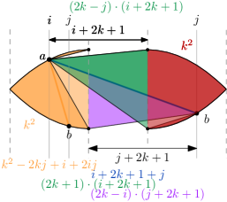
(a) Decomposition of the edges for case 1.page

(b) Decomposition of the edges for case 2.page

Figure 18: Decomposition of the edges for the upper bounds.

$$|T| =k^{2}\ +\ (2k-j)(i+2k+1)\ +\ (i+2k+1+j)\ +\ (2k-i)(2k+1+j)\ +\ k^{2}$$

$$=10k^{2}+6k+1-2ij\leq 10k^{2}+6k+1$$

with equality if and only if either $a$ or $b$ (or both) lie on the boundary of the large gap. In the second case, since $a$ is to the left of $b$ we have $i>j$ and similar algebra, see fig:flatboundcase2, gives

$$|T|=(k^{2}-2kj+i+2ij)\ +\ (2k+1)(2k+1+i)\ +\ k^{2}.$$

Since the right-hand side is increasing in $i$ and $i\leq k$, we get

$$|T|\leq(k^{2}+k)+(2k+1)(3k+1)+k^{2}=8k^{2}+6k+1$$

which is less than the claimed upper bound $10k^{2}+6k+1$ by a margin.

5 Polynomial time algorithms for special cases

page

In subsec:dpbistar we show that the longest plane tree of diameter at most $3$ can be computed in polynomial time. Such a tree may be relevant in providing an approximation algorithm with a better approximation factor, but its computation is not trivial, even in the case of flat point sets.

In sec:diam4 we show how to compute in polynomial time a longest plane tree among those of the following form: all the points are connected to three distinguished points on the boundary of the convex hull. Again, such a tree may play an important role in designing future approximation algorithms, as intuitively it seems to be better than the three stars considered in our previous approximation algorithm, when there is a point in the far region.

5.1 Finding the longest tree of diameter 3

page For any two points $a,b$ of $\mathcal{P}$, a bistar rooted at $a$ and $b$ is a tree that contains the edge $ab$ and where each point in $\mathcal{P}\setminus\{a,b\}$ is connected to either $a$ or $b$. Note that stars are also bistars. In this section we prove the following theorem.

See 1.6

Proof 5.1.

Note that each bistar has diameter at most 3. Conversely, each tree with diameter three has one edge $uv$ where each point $p\in\mathcal{P}$ has distance at most $1$ to either $u$ or $v$. It follows that all trees with diameter at most three are bistars. In lem:bestbistar we show that for any two fixed points $a$, $b$, the longest plane bistar rooted at $a$ and $b$ can be computed in time $\mathcal{O}(n^{2})$. By iterating over all possible pairs of roots and taking the longest such plane bistar, we find the longest plane spanning tree with diameter at most $3$ in time $\mathcal{O}(n^{4})$.

We now describe the algorithm used to find the longest plane bistar rooted at two fixed points $a$ and $b$. Without loss of generality we can assume that the points $a$ and $b$ lie on a horizontal line with $a$ to the left of $b$. Furthermore, as we can compute the best plane bistar above and below the line through $a$ and $b$ independently, we can assume that all other points lie above this horizontal line. In order to solve this problem by dynamic programming, we consider a suitable subproblem.

Figure 19: Two examples of valid pairs $p,q$ with their quadrilaterals $Q(p,q)$ shaded.page

The subproblems considered in the dynamic program are indexed by an ordered pair $p,q$ of different points of $\mathcal{P}$ such that the edges $ap$ and $bq$ do not cross. A pair $p,q$ satisfying these condition is a valid pair. For each valid pair $p,q$, note that the segments $ap$, $pq$, $qb$ and $ba$ form a simple (possibly non-convex) polygon. Let $Q(p,q)$ be the portion of this polygon below the horizontal line $y=\min\{y(p),y(q)\}$, as shown in fig:dp_bistar_subproblem. We define the value $Z(p,q)$ to be the length of the longest plane bistar rooted at $a$ and $b$ on the points in the interior of $Q(p,q)$, without counting $\|ab\|$. If there are no points of $\mathcal{P}$ within the quadrilateral $Q(p,q)$, we set $Z(p,q)=0$.

Consider the case when the quadrilateral $Q(p,q)$ contains some points, and let $k_{p,q}$ be the highest point of $\mathcal{P}$ inside of $Q(p,q)$. Then we might connect $k_{p,q}$ either to $a$ or to $b$. By connecting it to $a$, we force all points in the triangle $L_{p,q}$ defined by the edges $ap$ and $ak_{p,q}$ and the line $y=y(k_{p,q})$, to be connected to $a$. Similarly, when connecting $k_{p,q}$ to $b$, we enforce the triangle $R_{p,q}$ defined by $bq$, $bk_{p,q}$ and the line $y=y(k_{p,q})$. See fig:dp_bistar_recurrence for an illustration. In the former case we are left with the subproblem defined by the valid pair $k_{p,q},q$, while in the latter case we are left with the subproblem defined by the valid pair $p,k_{p,q}$. Formally, for each valid pair $p,q$ we have the following recurrence:

$$Z(p,q)=\begin{cases}0&\text{if no point of $\mathcal{P}$ is in $Q(p,q)$,}\\ \max\begin{cases}Z(k_{p,q},q)+\|ak_{p,q}\|+\sum_{l\in L_{p,q}}\|al\|\\ Z(p,k_{p,q})+\|bk_{p,q}\|+\sum_{r\in R_{p,q}}\|br\|\end{cases}&\text{otherwise.}\end{cases}$$

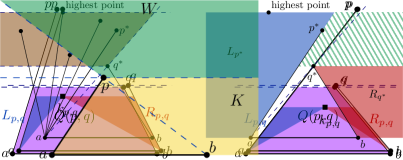
Figure 20: Fixing $k_{p,k}$ gives two possible triangular regions where edges are fixed.page

Lemma 5.2.

page Using $Z(p,q)$ for all valid $p,q$ we can find a best plane bistar rooted at $a$ and $b$.

Proof 5.3.

Consider a fixed best plane bistar and assume, without loss of generality, that the highest point is connected to $a$; the other case is symmetric. Let $q^{*}$ be the highest point that is connected to $b$; if $q^{*}$ does not exist then the bistar degenerates to a star rooted at $a$. This means that all the points above $q^{*}$ are attached to $a$. Let $p^{*}$ be the point above $q^{*}$ that, circularly around $a$, is closest to $ab$. See fig:dp_bistar_p*. Note that $p^{*},q^{*}$ is a valid pair and all the points above $q^{*}$ are to the left of $ap^{*}$. For $p\in\mathcal{P}$, denote by $L_{p}$ the set of points in $\mathcal{P}$ that, circularly around $a$, are to the left of $ap$. Similarly, denote by $R_{q}$ the set of points in $\mathcal{P}$ below $q$ and to the right of $bq$, when sorted circularly around $b$. See fig:dp_bistar_p*, right. The length of this optimal plane bistar rooted at $a$ and $b$ is then

$$\left(\sum_{l\in L_{p^{*}}}\|al\|\right)+\left(\sum_{r\in R_{q^{*}}}\|br\|\right)+\|ap^{*}\|+\|bq^{*}\|+\|ab\|+Z(p^{*},q^{*}).$$

On the other hand, each of the values of the form

$$\left(\sum_{l\in L_{p}}\|al\|\right)+\left(\sum_{r\in R_{q}}\|br\|\right)+\|ap\|+\|bq\|+\|ab\|+Z(p,q),\cref@constructprefix{page}{\cref@result}$$ (11)

where $p$, $q$ is a valid pair of points such that $y(p)>y(q)$, is the length of a plane, not necessarily spanning, bistar rooted at $a$ and $b$. (It is not spanning, if there is some point above $q$ and right of $ap$.)

Taking the maximum of $|S_{a}|$ and equation (11) over the valid pairs $p,q$ such that $y(p)>y(q)$ gives the longest plane bistar for which the highest point is connected to $a$. A symmetric formula gives the best plane bistar if the highest point is connected to $b$. Taking the maximum of both cases yields the optimal value.

Figure 21: Left: The point $p^{*}$ is the point of $\mathcal{P}$ in the shaded region that is angularly around $a$ closest to $q^{*}$. Right: the regions $L_{p^{*}}$ and $R_{q^{*}}$ are shaded. The region with bars is empty.page

The actual edges of the solution can be backtracked by standard methods.

Lemma 5.4.

page The algorithm described in the proof of lem:bistarcorrect can be implemented in time $\mathcal{O}(n^{2})$.

Proof 5.5.

A main complication in implementing the dynamic program and evaluating (11) efficiently is finding sums of the form $\sum_{l\in\Delta\cap\mathcal{P}}\|al\|$ or $\sum_{r\in\Delta\cap\mathcal{P}}\|br\|$, and the highest point in $\Delta\cap\mathcal{P}$, where $\Delta$ is a query triangle (with one vertex at $a$ or $b$). These type of range searching queries can be handled using standard data structures [ColeY84, Matousek93]: after preprecessing $\mathcal{P}$ in time $\mathcal{O}(n^{2}\operatorname{polylog}n)$, any such query can be answered in $\mathcal{O}(\operatorname{polylog}n)$ time. Noting that there are $\mathcal{O}(n^{2})$ such queries, a running time of $\mathcal{O}(n^{2}\operatorname{polylog}n)$ is immediate. However exploiting our specific structure and using careful bookkeeping we can get the running time down to $\mathcal{O}(n^{2})$.

As a preprocessing step, we first compute two sorted lists $\mathcal{L}_{a}$ and $\mathcal{L}_{b}$ of $\mathcal{P}\setminus\{a,b\}$. The list $\mathcal{L}_{a}$ is sorted angular at $a$ and $\mathcal{L}_{b}$ is sorted by the angle at $b$.

The values $\sum_{l\in L_{p}}\|al\|$ and $\sum_{r\in R_{q}}\|br\|$ (as depicted in fig:dp_bistar_p*) for all $p,q\in\mathcal{P}$ can be trivially computed in $\mathcal{O}(n^{2})$ time: there are $\mathcal{O}(n)$ such values and for each of them we can scan the whole point set to explicitly get $L_{p}$ or $R_{q}$ in $\mathcal{O}(n)$ time. There are faster ways of doing this, but for our result this suffices.

Assuming that the values $Z(p,q)$ are already available for all valid pairs $p$, $q$, we can evaluate (11) in constant time. For any two points $p$, $q$ we check whether they form a valid pair and whether $y(p)>y(q)$ in constant time. We can then either evaluate (11) or the symmetric formula again in constant time. Thus, in $\mathcal{O}(n^{2})$ time we obtain the optimal solution.

It remains to compute the values $Z(p,q)$ for all valid pairs $p$, $q$. First, we explain how to compute all the triples of the form $(p,q,k_{p,q})$ for all valid pairs $p,q$ in $\mathcal{O}(n^{2})$ time. Then we group these triples in a clever way to implement the dynamic program efficiently.

We focus on the triples with $y(p)<y(q)$ and show how to find the triples of the form $(p,\cdot,\cdot)$ for a fixed $p$. The case with $y(p)>y(q)$ and a fixed $q$ is symmetric. Let $W$ be the points of $\mathcal{P}$ to the right of the ray $bp$ above the horizontal line $y=y(p)$. Furthermore let $K$ be the points of $\mathcal{P}$ to the right of $ap$ and with $y$ coordinate between $y(a)$ and $y(p)$. An illustration of $W$ and $K$ can be found in fig:dp_bistar_W. Any point $q$ with $y(q)>y(p)$ forms a valid pair $p,q$ if and only if $q$ lies in $W$. The point $k_{p,q}$ must lie in $K$ by its definition.

Figure 22: Left: The regions defining $W$ and $K$ for fixed $a$, $b$ and $p$.page

We use $\mathcal{L}_{b}$ to find the triples $(p,\cdot,\cdot)$. We iterate through the list in clockwise order starting at the ray $ba$ and keep track of the highest $k^{*}\in K$ encountered so far. If the current point lies in $\mathcal{P}\setminus(K\cup W)$ we simply skip it. If the current point lies in $K$ we update $k^{*}$ if necessary. Finally, if the current point lies in $W$, we report the triple $(p,q,k^{*}=k_{p,q})$.

For a fixed $p$ we only iterate $\mathcal{L}_{b}$ once. Thus, for this fixed $p$ the running time for finding all triples $(p,q,k_{p,q})$ with $p,q$ forming a valid pair and $y(p)<y(q)$ is $\mathcal{O}(n)$. By the procedure we just described and its symmetric procedure on all $p\in\mathcal{P}\setminus\{a,b\}$ we find all the triples $(p,q,k_{p,q})$ where $p,q$ is a valid pair in overall $\mathcal{O}(n^{2})$ time.

To compute $Z(p,q)$ for all valid pairs using dynamic programing, we also need to compute the corresponding values $\sum_{l\in L_{p,q}}\|al\|$ and $\sum_{r\in R_{p,q}}\|br\|$. Refer to fig:dp_bistar_recurrence to recall the definition of $L_{p,q}$ and $R_{p,q}$. For the following procedure we shift the focus to the point $k$. For each point $k\in\mathcal{P}\setminus\{a,b\}$ we collect all triples $(p,q,k=k_{p,q})$, and compute the sums $\sum_{l\in L_{p,q}}\|al\|$ and $\sum_{r\in R_{p,q}}\|br\|$ in linear time for each fixed $k$, as follows.

We concentrate on the first type of sum, $\sum_{l\in L_{p,q}}\|al\|$, where $q$ has no role, as the sum is defined by $p$ and $k$. For the following description we assume that $\mathcal{L}_{a}$ is sorted in counterclockwise order. We create a (sorted) subsequence $\mathcal{L}_{a}^{k}$ of $\mathcal{L}_{a}$ containing only the points with $y$ coordinate below $y(k)$ and an angle at $a$ larger than $\sphericalangle bak$. We iterate over the elements of $\mathcal{L}_{a}$, starting at the successor of $k$. While iterating we maintain the last element from $\mathcal{L}_{a}^{k}$ we have seen and the prefix sum $\sum_{l}\|al\|$ of all points $l$ in $\mathcal{L}_{a}^{k}$ we encountered so far. When advancing to the next point $p$ in $\mathcal{L}_{a}$ there are two possibilities. If $p$ also lies in $\mathcal{L}_{a}^{k}$ we advance in $\mathcal{L}_{a}^{k}$ and update the prefix sum. Otherwise, we can report $\sum_{l\in L_{p,q^{\prime}}}\|al\|$ to be the current prefix sum for all $q^{\prime}$ in a triple $(p,q^{\prime},k)$.

For any fixed $k$ this needs at most two iterations through the list $\mathcal{L}_{a}$ and can thus be executed in $\mathcal{O}(n)$ time. A symmetric procedure can be carried out for $\sum_{r\in R_{p,q}}\|br\|$ using $\mathcal{L}_{b}$. As in the case for finding the triples, this results in $\mathcal{O}(n^{2})$ overall time to compute all relevant sums $\sum_{l\in L_{p,q}}\|al\|$ and $\sum_{r\in R_{p,q}}\|br\|$.

Now we can implement the dynamic program in the straightforward way. Using the precomputed information we spend $\mathcal{O}(1)$ time for each value $Z(p,q)$, for a total running time of $\mathcal{O}(n^{2})$.

5.2 Extending the approach to special trees of diameter 4

page Now we show how we can extend the ideas to get a polynomial time algorithm for special trees with diameter $4$. Given three points $a,b,c$ of $\mathcal{P}$, a tristar rooted at $a,b$ and $c$ is a tree such that each edge has at least one endpoint at $a$, $b$ or $c$. We show the following:

See 1.7

Proof 5.6.

Let $a,b,c$ be the specified points on the boundary of the convex hull of $\mathcal{P}$. We have to compute the longest plane tristar rooted at $a,b$ and $c$. We assume, without loss of generality, that the edges $ac$ and $bc$ are present in the tristar; the other cases are symmetric. We further assume that $a$ and $b$ lie on a horizontal line, with $a$ to the left of $b$.

The regions to the left of $ac$ and to the right of $bc$, as depicted in fig:tristarexclude, can be solved independently of the rest of the instance. Indeed, the presence of the edges $ac$ and $bc$ blocks any edge connecting a point in one of those regions to a point outside the region. Each one of these regions can be solved as plane bistars, one rooted at $a,c$ and one rooted at $b,c$. It remains to solve the problem for the points enclosed by $ac$, $cb$ and the portion of the boundary of the convex hull from $b$ to $a$ (clockwise). Let $Q$ be this region. The problem for $Q$ can also be solved independently of the other problems. We assume for the rest of the argument that all points of $\mathcal{P}$ are in $Q$.

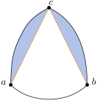
Figure 23: The regions cut off by $ac$ and $bc$ can be solved independently as bistars.page

For solving the problem for $Q$ we will use a variation of the dynamic programming approach for bistars. For any two points $p,q$ of $\mathcal{P}$, let us write $p\preceq_{c}q$ when in the counterclockwise order around $c$ we have the horizontal ray through $c$ to the left, then $cp$ and then $cq$ or the segments $cp$ and $cq$ are collinear. (Since we assume general position, the latter case occurs when $p=q$.)

The subproblems for the dynamic program are defined by a five tuple $(p,p^{\prime},r,q^{\prime},q)$ of points of $\mathcal{P}$ such that

• $p^{\prime}$ and $q^{\prime}$ are distinct;

• $p\preceq_{c}p^{\prime}\preceq_{c}r\preceq_{c}q^{\prime}\preceq_{c}q$; and

• $p^{\prime}$ and $q^{\prime}$ are contained in the closed triangle $cpq$.

One such five tuple is a valid tuple, see fig:ds-tristar1. Note that the first and the second condition imply that $ap$ and $bq$ do not cross. Some of the points may be equal in the tuple; for example we may have $p=p^{\prime}$ or $p^{\prime}=r$ or even $p=p^{\prime}=r$. For each valid tuple $(p,p^{\prime},r,q^{\prime},q)$, let $Q(p,r,q)$ be the points of $\mathcal{P}$ contained in $Q$ below the polygonal path $ap$, $pq$ and $qb$, and below the horizontal line through the lowest of the points $p,q,r$. Note that the point $r$ is used only to define the horizontal line.

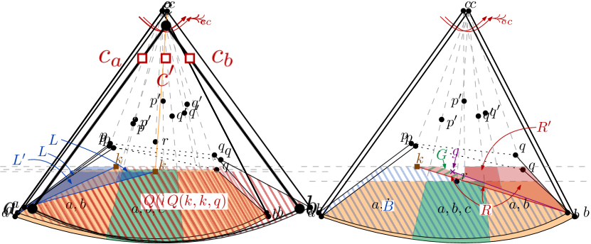
Figure 24: Two examples of valid tuples $(p,p^{\prime},r,q^{\prime},q)$ with the region $Q(p,r,q)$ shaded. Each $Q(p,r,q)$ is split into 3 regions telling, for each of them, which roots can be used for that region.page

For each valid tuple $(p,p^{\prime},r,q^{\prime},q)$, we define $Z(p,p^{\prime},r,q^{\prime},q)$ as the length of the optimal plane tristar rooted at $a$, $b$, $c$ for the points in the interior of $Q(p,r,q)$, without counting $\|ac\|+\|bc\|$, and with the additional restriction that a point $k$ can be connected to $c$ only if $p^{\prime}\preceq_{c}k\preceq_{c}q^{\prime}$. This last condition is equivalent to telling that no edge incident to $c$ in the tristar can cross $ap^{\prime}$ or $bq^{\prime}$. Thus, we are looking at the length of the longest plane graph in which each point in the interior of $Q(p,r,q)$ must be connected to either $a$, $b$ or $c$, and no edge crosses $ap^{\prime}$ or $bq^{\prime}$.

If $Q(p,r,q)$ has no points, then $Z(p,p^{\prime},r,q^{\prime},q)=0$. If $Q(p,r,q)$ has some point, we find the highest point $k=k(p,r,q)$ in $Q(p,r,q)$ and consider how it may attach to the roots and which edges are enforced by each of these choices. We can always connect $k$ to $a$ or $b$, as $Q(p,r,q)$ is free of obstacles. If $p^{\prime}\preceq_{c}k\preceq_{c}q^{\prime}$, then we can connect $k$ to $c$. If $k$ is connected to $c$ it only lowers the boundary of the region $Q(\cdot,\cdot,\cdot)$ that has to be considered. However if $k$ is connected to $a$ or $b$, it splits off independent regions, some of them can be attached to only one of the roots, some of them are essentially a bistar problem rooted at $c$ and one of $a,b$. To state the recursive formulas precisely, for a region $R$ and roots $z,c$, let $\mathrm{BS}_{z,c}(R)$ be the length of the optimal plane bistar rooted at $z,c$ for the points in $R$. Such a value can be computed using lem:bistarcorrect.

Formally the recurrence for $Z(p,p^{\prime},r,q^{\prime},q)$ looks as follows. If $Q(p,r,q)$ is empty, then $Z(p,p^{\prime},r,q^{\prime},q)=0$. If $Q(p,r,q)$ is not empty, let $k$ be the highest point of $Q(p,r,q)$; we have three subcases:

Case 1: $k\prec_{c}p^{\prime}$.

Let $L$ be the points of $Q(p,r,q)$ above $ak$. Let $B$ be the points of $Q(p,r,q)$ below $bk$ and let $G$ be the points $t$ of $Q(p,r,q)\setminus B$ such that $k\prec_{c}t\prec_{c}p^{\prime}$. Let $g$ be the point with largest angle at $b$ among the points in $G$. Then we define $R^{\prime}$ to be the set of all points $t$ in $Q(p,r,q)\setminus B$ with $p^{\prime}\prec_{c}t\prec_{c}q^{\prime}$ which are above $gb$. Finally let $R=Q(p,q,r)\setminus(B\cup R^{\prime})$, as shown in fig:ds-tristar2. We get the following recurrence in this case:

$$Z(p,p^{\prime},r,q^{\prime},q)=\max\begin{cases}Z(k,p^{\prime},r,q^{\prime},q)+\|ak\|+\sum_{l\in L}\|al\|\\ \mathrm{BS}_{a,b}(B)+\|bk\|+\mathrm{BS}_{b,c}(R^{\prime})+\sum_{r\in R}\|br\|\end{cases}$$

Case 2: $p^{\prime}\prec_{c}k\prec_{c}q^{\prime}$.

Let $L^{\prime}$ be the points $t$ of $Q(p,r,q)$ above $ak$ such that $t\prec_{c}p^{\prime}$ and let $L$ be the points $t$ of $Q(p,r,q)$ above $ak$ such that $p^{\prime}\prec_{c}t\prec_{c}k$. Furthermore, let $R$ be the points $t$ of $Q(p,r,q)$ above $bk$ such that $k\prec_{c}t\prec_{c}q^{\prime}$, and let $R^{\prime}$ be the points $t$ of $Q(p,r,q)$ above $bk$ such that $q^{\prime}\prec_{c}t$; see fig:ds-tristar3. We get the following recurrence in this case:

$$Z(p,p^{\prime},r,q^{\prime},q)=\max\begin{cases}Z(p,p^{\prime},k,q^{\prime},q)+\|ck\|\\ Z(k,k,k,q^{\prime},q)+\|ak\|+\mathrm{BS}_{a,c}(L)+\sum_{l\in L^{\prime}}\|al\|\\ Z(p,p^{\prime},k,k,k)+\|bk\|+\mathrm{BS}_{b,c}(R)+\sum_{r\in R^{\prime}}\|br\|\end{cases}$$

Case 3: $q^{\prime}\prec_{c}k$.

The case is symmetric to the case $k\prec_{c}p^{\prime}$.

Figure 25: The two cases in the recurrence when $k\prec_{c}p^{\prime}$.page

Figure 26: One of the cases in the recurrence when $p^{\prime}\prec_{c}k\prec_{c}q^{\prime}$.page

Figure 27: Starting Casepage

The values $Z(p,p^{\prime},r,q^{\prime},q)$ for all valid tuples $(p,p^{\prime},r,q^{\prime},q)$ can be computed using dynamic programming and the formulas described above. The dynamic program is correct by a simple but tedious inductive argument.

Note that we have to compute a few solutions for bistars. In the recursive calls these have the form $\mathrm{BS}_{z,c}(R)$ for $z\in\{a,b\}$ and some region $R$ of constant size description. More precisely, each such region is defined by two points of $\mathcal{P}$ (case of $L$ in fig:ds-tristar3) or by four points of $\mathcal{P}$ (case of $R$ in fig:ds-tristar2, where it is defined by $k,g,q^{\prime},q$). Thus, we have $\mathcal{O}(n^{4})$ different bistar problems, and each of them can be solved in polynomial time using lem:bistarcorrect.

To compute the optimal plane tristar, we add three dummy points to $\mathcal{P}$ before we start the dynamic programming. We add a point $c_{a}$ on the edge $ac$ arbitrarily close to $c$, a point $c_{b}$ on the edge $bc$ arbitrarily close to $c$, and a point $c^{\prime}$ between $c_{a}$ and $c_{b}$, see fig:ds-tristar4. We perturb the points $c_{a},c^{\prime}$ and $c_{b}$ slightly to get them into general position. Note that $(c_{a},c_{a},c^{\prime},c_{b},c_{b})$ is a valid tuple. We can now compute $Z(c_{a},c_{a},c^{\prime},c_{b},c_{b})$ by implementing the recurrence with standard dynamic programming techniques in polynomial time. By adding $\|ac\|$, $\|bc\|$ and the lengths of the independent bistars from fig:tristarexclude to $Z(c_{a},c_{a},c^{\prime},c_{b},c_{b})$, we get the length of the longest plane tristar rooted at $a,b$ and $c$.

Similar to the proof thm:dp we can iterate over all possible triples of specified points to find the best plane tristar rooted at the boundary of the convex hull.

6 Local improvements fail

page

In this section we prove that the following natural algorithm AlgLocal($\mathcal{P}$) based on local improvements generally fails to compute the longest plane tree.

Algorithm AlgLocal($\mathcal{P}$):

1. Construct an arbitrary plane spanning tree $T$ on $\mathcal{P}$.

2. While there exists a pair of points $a$, $b$ such that $T\cup ab$ contains an edge $cd$ with $|cd|<|ab|$ and $T\cup\{ab\}\setminus\{cd\}$ is plane:

   1. Set $T\to T\cup\{ab\}\setminus\{cd\}$. // tree $T\cup ab\setminus\{cd\}$ is longer than $T$

3. Output $T$.

Lemma 6.1.

page For certain point sets $\mathcal{P}$ the algorithm AlgLocal($\mathcal{P}$) fails to compute the longest plane tree.

Proof 6.2.

We construct a point set $\mathcal{P}$ consisting of $9$ points to show the claim. The first three points of $\mathcal{P}$ are the vertices of an equilateral triangle. We assume that two of these vertices are on a horizontal line and denote by $x$ the center of this triangle. Let $r_{0}$ be the circumradius of the triangle.

Inside of this triangle, we want to place the vertices of two smaller equilateral triangles, where again the smaller is contained in the larger one. Set $\alpha=17^{\circ},r_{1}=\frac{2}{3}r_{0}$ and $r_{2}=\frac{1}{3}r_{0}$. We then place the first of the additional triangles on the circle $\partial D(x,r_{1})$ in a way that the vertices have an angle of $\alpha$ to the nearest angular bisector of the outer triangle. We place the second additional triangle on the circle $\partial D(x,r_{2})$ again with an angle to the nearest bisector of the outer triangle. However this time, the angle is $\alpha/2$. This construction is visualized in fig:stuckconst.

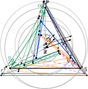
Figure 28: Construction of the point setpage

Now consider the tree on this point set depicted by the solid edges in fig:stucktree. Note that the green, blue and yellow edges are rotational symmetric. The edges depicted in purple in fig:stucktree are representative for the possible edges currently not in the tree, which connect the outer to the inner triangle. However as they are either the smallest edges in the cycle or intersect some edge not in a cycle, the algorithm cannot choose $ab$ to be one of those edges.

(a) A tree which cannot be locally improvedpage

(b) A tree where each pair of edges in the same color is at least as long as the matching pair in fig:stucktreepage

Figure 29: The algorithm AlgLocal($\mathcal{P}$) can get stuck.page

The possible edges connecting the outer to the middle triangle are depicted in red. The red edge $pq$ is not in a cycle with the edge it crosses, and thus it is not a possible swap keeping planarity. For the second red edge and the possible edges connecting the middle to the inner triangle, it can similarly be seen that they are shorter than any edge of the current tree. Finally, for the edges along the triangles or the edges connecting the interior and the middle triangle, it can easily be verified that there will be no strictly smaller edge in the unique cycle closed by them.

On the other hand, in the tree depicted in fig:stucklonger each pair of same colored edges is longer than its counterpart in fig:stucktree. Therefore AlgLocal($\mathcal{P}$) does not yield a correct result.

7 Conclusions

We leave several open questions:

1. What is the correct approximation factor of the algorithm AlgSimple($\mathcal{P}$) presented in sec:approximation? While each single lemma in sec:approximation is tight for some case, it is hard to believe that the whole analysis, leading to the approximation factor $f\doteq 0.5467$, is tight. We conjecture that the algorithm has a better approximation guarantee.

2. What is the approximation factor $\operatorname{BoundDiam}(3)$ achieved by the polynomial time algorithm that outputs the longest plane tree with diameter 3? By thm:diameter-3-bound it is at most $5/6$ (and by [1] it is at least $1/2$).

3. For a fixed diameter $d\geq 4$, is there a polynomial-time algorithm that outputs the longest plane tree with diameter at most $d$? By thm:dp we know the answer is yes when $d=3$. And thm:tristar gives a positive answer for special classes of trees with diameter $4$. Note that a hypothetical polynomial-time approximation scheme (PTAS) has to consider trees of unbounded diameter because of thm:diameter-bound. It is compatible with our current knowledge that computing an optimal plane tree of diameter, say, $\mathcal{O}(1/\varepsilon)$ would give a PTAS.

4. Is the general problem of finding the longest plane tree in P? A similar question can be asked for several other plane objects, such as paths, cycles, matchings, perfect matchings, or triangulations. The computational complexity in all cases is open.

References

- [1] Noga Alon, Sridhar Rajagopalan, and Subhash Suri. Long non-crossing configurations in the plane. Fundam. Inform., 22(4):385–394, 1995. \hrefhttp://dx.doi.org/10.3233/FI-1995-2245 \pathdoi:10.3233/FI-1995-2245.
- [2] Sanjeev Arora. Polynomial time approximation schemes for Euclidean traveling salesman and other geometric problems. J. ACM, 45(5):753–782, 1998. URL: