Refining activation downsampling with SoftPool

Abstract

Convolutional Neural Networks (CNNs) use pooling to decrease the size of activation maps. This process is crucial to increase the receptive fields and to reduce computational requirements of subsequent convolutions. An important feature of the pooling operation is the minimization of information loss, with respect to the initial activation maps, without a significant impact on the computation and memory overhead. To meet these requirements, we propose SoftPool: a fast and efficient method for exponentially weighted activation downsampling. Through experiments across a range of architectures and pooling methods, we demonstrate that SoftPool can retain more information in the reduced activation maps. This refined downsampling leads to improvements in a CNN’s classification accuracy. Experiments with pooling layer substitutions on ImageNet1K show an increase in accuracy over both original architectures and other pooling methods. We also test SoftPool on video datasets for action recognition. Again, through the direct replacement of pooling layers, we observe consistent performance improvements while computational loads and memory requirements remain limited.

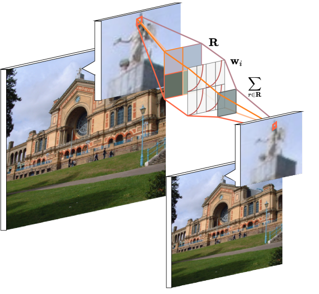
Figure 1: SoftPool illustration. The original image is sub-sampled with a $2\!\times\!2$ ($k\!\!=\!\!2$) kernel. The output is based on the exponentially weighted sum of the original pixels within the kernel region. This can improve the representation of high-contrast regions, present around object edges or specific feature activations.

1 Introduction

Pooling layers are essential in convolutional neural networks (CNNs) to decrease the size of activation maps. They reduce the computational requirements of the network while also achieving spatial invariance, and increase the receptive field of subsequent convolutions [6, 25, 41].

A range of pooling methods has been proposed, each with different properties (see Section 2). Most architectures use maximum or average pooling, both of which are fast and memory-efficient but leave room for improvement in terms of retaining important information in the activation map.

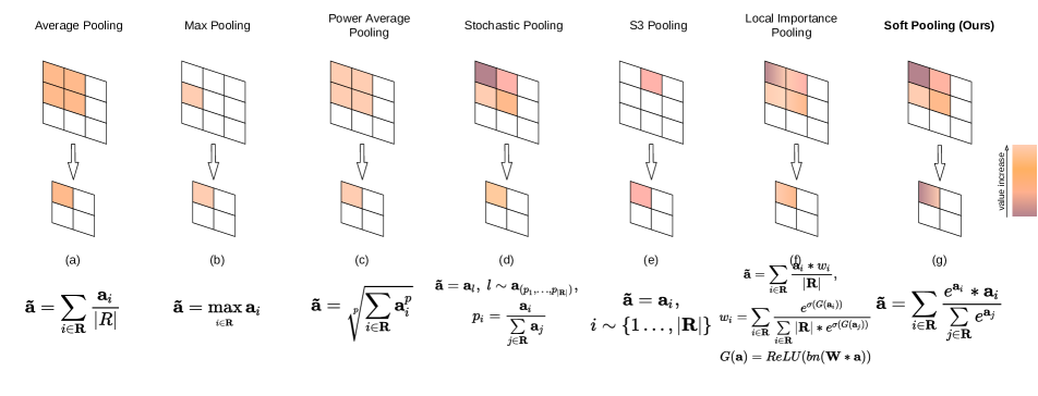
Figure 2: Pooling variants. $\mathbf{R}$ is the set of pixel values in the kernel neighborhood. (a,b) Average and maximum pooling are based on averaging and maximum activation selection in a kernel. (c) Power Average pooling ($L_{p}$) [10, 14] is proportional to average pooling raised to a power ($p$). The output is equal to max-pool for $p\rightarrow\infty$, and sum pooling when $p=1$. (d) Stochastic pooling [45] outputs a randomly selected activation from the kernel region. (e) Stochastic Spatial Sampling (S3Pool) [46] samples random horizontal and vertical regions given a specified stride. (f) Local Importance Pooling (LIP) [12] uses a trainable sub-net $G$ to enhance specific features. (g) SoftPool (ours) exponentially weighs the effect of activations using a softmax kernel.

We introduce SoftPool, a kernel-based pooling method that uses the softmax weighted sum of activations. We demonstrate that SoftPool largely preserves descriptive activation features, while remaining computationally and memory-efficient. Owing to better feature preservation, models that include SoftPool consistently show improved classification performance compared to their original implementations. We make the following contributions:

• We introduce SoftPool: a novel pooling method based on softmax normalization that can be used to downsample 2D (image) and 3D (video) activation maps.

• We demonstrate how SoftPool outperforms other pooling methods in preserving the original features, measured using image similarity.

• Experimental results on image and video classification tasks show consistent improvement when replacing the original pooling layers by SoftPool.

The remainder of the paper is structured as follows. We first discuss related work on feature pooling. We then detail SoftPool (Section 3) and evaluate it in terms of feature loss and image and video classification performance over multiple pooling methods and architectures (Section 4).

2 Related Work

Pooling for hand-crafted features. Downsampling is a widely used technique in hand-coded feature extraction methods. In Bag-of-Words (BoW) [7], images were viewed as collections of local patches, pooled and encoded as vectors [38]. Combinations with Spatial Pyramid Matching [20] aimed to preserve spatial information. Later works considered the selection of the maximum SIFT features in a spatial region [42]. Pooling has primarily been linked to the use of max-pooling, because of the feature robustness of biological max-like cortex signals [29]. Boureau et al. [2] studied maximum and average pooling in terms of their robustness and usability, and found max-pooling to produce representative results in low feature activation settings.

Pooling in CNNs. Pooling has also been adapted to learned feature approaches, as seen in early works in CNNs [21]. The main benefit of pooling has traditionally been the creation of condensed feature representations which reduce the computational requirements and enable the creation of larger and deeper architectures [30, 34].

Recent efforts have focused on preserving relevant features during downsampling. An overview of a number of popular pooling methods appears in Figure 2. Initial approaches include stochastic pooling [45], which uses a probabilistic weighted sampling of activations within a kernel region. Mixed pooling based on maximum and average pooling has been used either probabilistically [43] or through a combination of portions from each method [22]. Based on the combination of averaging and maximization, Power Average ($L_{p}$) pooling [10, 14] utilizes a learned parameter $p$ to determine the relative importance of both methods. When $p=1$, the local sum is used, while $p\rightarrow\infty$ corresponds to max-pooling. More recent approaches have considered grid-sampling methods. In S3Pool [46], the downsampled outputs stem from randomly sampling the rows and columns of the original feature map grid. Methods that depend on learned weights include Detail Preserving Pooling (DPP, [28]) that uses average pooling while enhancing activations with above-average values. Local Importance Pooling (LIP, [12]) utilizes learned weights as a sub-network attention-based mechanism. Other learned pooling approaches such as Ordinal Pooling [8], which order kernel pixels in discerningly and assigning them trainable weights. More recently, Zhao and Snoek [48] proposed a pooling technique named LiftPool based on the use of four different learnable sub-bands of the input. The produced output is composed by a mixture of the discovered sub-bands.

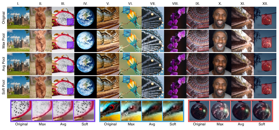
Figure 3: Examples of maximum, average and soft pooling. Images are $1200\times 1200$ pixels with the $3\times$ pooled equivalents reduced to 12.5% of the original size. Image selection was based on overall contrast (I, III, V, VIII, XII), color (II, IV, VI, IX), detail (III, V, X, XI, XII) and texture (II, VII). Images on the bottom row are zoomed-in regions. A high resolution version of the regions appears alongside a detailed discussion in §1 of the Supplementary Material.

Most of the aforementioned methods rely on different combinations of maximum and average pooling. Instead of combining existing methods, our work is based on a softmax weighting approach to preserve the basic properties of the input while amplifying feature activations of greater intensity. SoftPool does not require trainable parameters, thus is independent to the training data used. Moreover, it is significantly more computational and memory efficient compared to learned approaches. In contrast to max-pooling, our approach is differentiable. Gradients are obtained for each input during backpropagation, which improves neural connectivity during training. Through the weighted softmax, pooled regions are also less susceptible to vanishing local kernel activations, a common issue with average pooling. We demonstrate the effects of SoftPool in Figure 3, where the zoomed-in regions show that features are not completely lost as with hard-max selection, or suppressed by the overall region through averaging.

3 SoftPool Downsampling

We start by formally introducing the forward flow of information in SoftPool and the gradient calculation during backpropagation. We consider a local region ($\mathbf{R}$) in an activation map ($\mathbf{a}$) with dimension $C\times H\times W$ with $C$ the number of channels, $H$ the height and $W$ the width of the activation map. For simplicity of notation, we omit the channel dimension and assume that $\mathbf{R}$ is the set of indices corresponding to the activations in the 2D spatial region under consideration. For a pooling filter of size $k\times k$, we consider $|\mathbf{R}|=k^{2}$ activations. The output of the pooling operation is $\tilde{\mathbf{a}}_{R}$ and the corresponding gradients are denoted with $\nabla\mathbf{\tilde{a}}_{i}$.

3.1 Exponential maximum kernels

SoftPool is influenced by the cortex neural simulations of Riesenhuber and Poggio [26] as well as the early pooling experiments with hand-coded features of Boureau et al. [2]. The proposed method is based on the natural exponent ($e$) which ensures that large activation values will have greater effect on the output. The operation is differentiable, which implies that all activations within the local kernel neighborhood will be assigned a proportional gradient, of at least a minimum value, during backpropagation. This is in contrast to pooling methods that employ hard-max or average pooling. SoftPool utilizes the smooth maximum approximation of the activations within kernel region $\mathbf{R}$. Each activation $\mathbf{a}_{i}$ with index $i$ is applied a weight $\mathbf{w}_{i}$ that is calculated as the ratio of the natural exponent of that activation with respect to the sum of the natural exponents of all activations within neighborhood R:

$$\mathbf{w}_{i}=\frac{e^{\mathbf{a}_{i}}}{\sum\limits_{j\in\mathbf{R}}e^{\mathbf{a}_{j}}}$$ (1)

The weights are used as non-linear transforms in conjunction with the value of the corresponding activation. Higher activations become more dominant than lower-valued ones. Because most pooling operations are performed in high-dimensional feature spaces, highlighting the activations with greater effect is a more balanced approach than simply selecting the average or maximum. In the latter case, discarding the majority of the activations presents the risk of losing important information. Conversely, an equal contribution of activations in average pooling can correspond to local intensity reductions by considering the overall regional feature intensity equally.

The output value of the SoftPool operation is produced through a standard summation of all weighted activations within the kernel neighborhood $\mathbf{R}$:

$$\tilde{\mathbf{a}}=\sum\limits_{i\in\mathbf{R}}\mathbf{w}_{i}*\mathbf{a}_{i}$$ (2)

In comparison to other max- and average-based pooling approaches, using the softmax of regions produces normalized results with a probability distribution proportional to the values of each activation with respect to the neighboring activations for the kernel region. This is in direct contrast to popular maximum activation value selection or averaging all activations over the kernel region, where the output activations are not regularized. A full forward and backward information flow is shown in Figure 4.

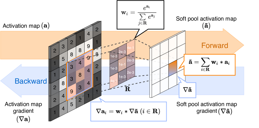
Figure 4: SoftPool calculation. In forward operation, in orange, the kernel uses the exponential softmax value of each activation as weight and calculates the weighted sum for region $\mathbf{R}$. These weights are also used for the gradients ($\nabla\tilde{\mathbf{a}}_{i}$), in blue. Activation gradients are proportional to the calculated softmax weights.

3.2 Gradient calculation

During the update phase in training, gradients of all network parameters are updated based on the error derivatives calculated at the proceeding layer. This creates a chain of updates, when backpropagating throughout the entire network architecture. In SoftPool, gradient updates are proportional to the weights calculated during the forward pass.

As softmax is differentiable, unlike maximum or stochastic pooling methods, during backpropagation, a minimum non-zero weight will be assigned to every positive activation within a kernel region. This enables the calculation of a gradient for every non-zero activation in that region, as shown in Figure 4.

In our implementation of SoftPool, we use finite ranges of possible values given a precision level (i.e., half, single or double) as detailed in §7 of the Supplementary Material. We retain the differentiable nature of softmax by assigning a lower arithmetic limit given the number of bits used by each type preventing arithmetic underflow.

3.3 Feature preservation

An integral goal of sub-sampling is the preservation of representative features in the input, while simultaneously minimizing the overall resolution. Creating unrepresentative downsampled versions of the original inputs can be harmful to the overall model’s performance as the representation of the input is detrimental for the task.

Currently widely used pooling techniques can be ineffective in certain cases, as shown in Figures 3 & 5. Average pooling decreases the effect of all activations in the region equally, while max pooling selects only the single highest activation in the region. SoftPool falls between the two, as all activations in the region contribute to the final output, with higher activations are more dominant than lower ones. This balances the effects of both average and max pooling, while leveraging the beneficial properties of both.

3.4 Spatio-temporal kernels

CNNs have also been extended to 3D inputs to include additional dimensions such as depth and time. To accommodate these inputs, we extend SoftPool to include an additional dimension. For an input activation map $\mathbf{a}$ of $C\times H\times W\times T$, with $T$ the temporal extent, we transform the 2D spatial kernel region R to a 3D spatio-temporal region with an additional third temporal dimension.

The produced output holds condensed spatio-temporal information. Issues that arise with the introduction of the temporal dimension are discussed and illustrated in §3 of the Supplementary Material. With the added dimension, desired pooling properties such as limited loss of information, a differentiable function, and low computational and memory overhead are even more important.

\begin{overpic}[width=496.85625pt]{figures/Pooling_comparison_examples.pdf} \put(24.7,9.7){\tiny{Original (HR)}} \put(33.1,9.7){\tiny{Average}} \put(39.4,9.7){\tiny{Maximum}} \put(47.0,9.7){\tiny{S3}\cite[cite]{[\@@bibref{}{zhai2017s3pool}{}{}]}} \par\put(24.5,0.8){\tiny{Stochastic} \cite[cite]{[\@@bibref{}{zeiler2013stochastic}{}{}]}} \put(32.5,0.8){\tiny{$L_{p}$} \cite[cite]{[\@@bibref{}{gulcehre2014learned}{}{}]}} \put(39.5,0.8){\tiny{Gate} \cite[cite]{[\@@bibref{}{lee2016generalizing}{}{}]}} \put(45.15,0.8){\tiny{SoftPool {(ours)}}} \par\par\put(73.1,9.7){\tiny{Original (HR)}} \put(81.5,9.7){\tiny{Average}} \put(87.8,9.7){\tiny{Maximum}} \put(95.4,9.7){\tiny{S3}\cite[cite]{[\@@bibref{}{zhai2017s3pool}{}{}]}} \par\put(72.9,0.8){\tiny{Stochastic} \cite[cite]{[\@@bibref{}{zeiler2013stochastic}{}{}]}} \put(80.9,0.8){\tiny{$L_{p}$} \cite[cite]{[\@@bibref{}{gulcehre2014learned}{}{}]}} \put(87.9,0.8){\tiny{Gate} \cite[cite]{[\@@bibref{}{lee2016generalizing}{}{}]}} \put(93.55,0.8){\tiny{SoftPool {(ours)}}} \par\end{overpic}

Figure 5: Visual comparisons over pooling methods. Both images are from Urban100 [17]. Left image (img024) shows high contrasting borders/edges. Right image (img078) presents the inverse of high local values within an overall low-valued region.

	Pooling method	DIV2K [1]						Urban100 [17]						Manga109 [23]
		$k=2$		$k=3$		$k=5$		$k=2$		$k=3$		$k=5$		$k=2$		$k=3$		$k=5$
		SSIM	PSNR	SSIM	PSNR	SSIM	PSNR	SSIM	PSNR	SSIM	PSNR	SSIM	PSNR	SSIM	PSNR	SSIM	PSNR	SSIM	PSNR
	Average	0.714	51.247	0.578	44.704	0.417	29.223	0.691	50.380	0.563	41.745	0.372	28.270	0.695	54.326	0.582	43.657	0.396	29.862
	Maximum	0.685	49.826	0.370	41.944	0.358	22.041	0.662	48.266	0.528	40.709	0.330	20.654	0.671	50.085	0.544	41.128	0.324	22.307
	Pow-average	0.419	35.587	0.286	26.329	0.178	16.567	0.312	31.911	0.219	24.698	0.124	15.659	0.381	29.248	0.276	18.874	0.160	9.266
	Sum	0.408	35.153	0.268	26.172	0.193	17.315	0.301	31.657	0.208	24.735	0.123	15.243	0.374	30.169	0.271	20.150	0.168	13.081
Trainable	$L_{p}$ [14]	0.686	49.912	0.542	43.083	0.347	25.139	0.676	48.508	0.534	39.986	0.326	26.365	0.675	51.721	0.561	41.824	0.367	27.469
	Gate [22]	0.689	50.104	0.560	43.437	0.353	25.672	0.675	49.769	0.537	40.422	0.328	26.731	0.679	51.980	0.569	42.127	0.374	27.754
	Lite-S3DPP [28]	0.702	50.598	0.562	44.076	0.396	27.421	0.684	49.947	0.551	40.813	0.365	27.136	0.691	52.646	0.573	42.794	0.386	28.598
	LIP [12]	0.711	50.831	0.559	44.432	0.401	28.285	0.689	50.266	0.558	41.159	0.370	27.849	0.689	53.537	0.579	43.018	0.391	29.331
Stoch.	Stochastic [45]	0.631	45.362	0.479	39.895	0.295	21.314	0.616	44.342	0.463	37.223	0.286	19.358	0.583	46.274	0.427	39.259	0.255	22.953
	S3 [46]	0.609	44.760	0.454	39.326	0.280	20.773	0.608	44.239	0.459	36.965	0.272	19.645	0.576	46.613	0.426	39.866	0.232	23.242
	SoftPool (Ours)	0.729	51.436	0.594	44.747	0.421	29.583	0.694	50.687	0.578	41.851	0.394	28.326	0.704	54.563	0.586	43.782	0.403	30.114

Table 1: Quantitative results on benchmark high-res datasets. Best results from each similarity measure are denoted in bold.

4 Experimental Results

We first evaluate the information loss for various pooling operators. We compare the downsampled outputs to the original inputs using standard similarity measures (Section 4.2). We also investigate each pooling operator’s computation and memory overhead (Section 4.3).

We then focus on the classification performance gain when using SoftPool in a range of popular CNN architectures and in comparison to other pooling methods (Section 4.4). We also perform an ablation study where we replace max-pooling operations by SoftPool operations in an InceptionV3 architecture (Section 4.5).

Finally, we demonstrate the merits of SoftPool for spatio-temporal data by focusing on action recognition in video (Section 4.6). Additionally, we investigate how transfer learning performance is affected when SoftPool is used.

4.1 Experimental settings

Datasets. For our experiments with images, we employ five different datasets for the tasks of image quality quantitative evaluation and classification. For image quality and similarity assessment we use high-resolution DIV2K [1], Urban100 [17], Manga109 [23], and Flicker2K [1]. ImageNet1K [27] is used for the classification task. For video-based action recognition, we use the large-scale HACS [47] and Kinetics-700 [3] datasets. Our transfer learning experiments are performed on the UCF-101 [31] dataset.

Training implementation details. For the image classification task, we perform random region selection of $294\times 294$ height and width, which was then resized to $224\times 224$. We use an initial learning rate of 0.1 with an SGD optimizer and a step-wise learning rate reduction every 40 epochs for a total of 100 epochs. The epochs number was chosen as no further improvements were observed for any of the models. We also set the batch size to 256 across all models.

For our experiments on videos, we use a multigrid training scheme [40], with frame sizes between 4–16 and frame crops of 90–256 depending on the cycle. On average, the video inputs are of size $8\times 160\times 160$. With the multigrid scheme, the batch sizes are between 64 and 2048 with each size counter-equal to the input size in every step to match the memory use. We use the same learning rate, optimizer, learning rate schedule and maximum number of epochs as in the image-based experiments.

Model	Params	GFLOP	Original		SoftPool (pre-train)		SoftPool (from scratch)
	(M)		top-1	top-5	top-1	top-5	top-1	top-5
ResNet18	11.7	1.83	69.76	89.08	70.56 (+0.80)	89.89 (+0.81)	71.27 (+1.51)	90.16 (+1.08)
ResNet34	21.8	3.68	73.30	91.42	74.03 (+0.73)	91.85 (+0.43)	74.67 (+1.37)	92.30 (+0.88)
ResNet50	25.6	4.14	76.15	92.87	76.60 (+0.45)	93.15 (+0.28)	77.35 (+1.17)	93.63 (+0.76)
ResNet101	44.5	7.87	77.37	93.56	77.74 (+0.37)	93.99 (+0.43)	78.32 (+0.95)	94.21 (+0.65)
ResNet152	60.2	11.61	78.31	94.06	78.73 (+0.42)	94.47 (+0.41)	79.24 (+0.92)	94.72 (+0.66)
DenseNet121	8.0	2.90	74.65	92.17	75.27 (+0.57)	92.60 (+0.43)	75.88 (+1.23)	92.92 (+0.75)
DenseNet161	28.7	7.85	77.65	93.80	78.12 (+0.47)	94.15 (+0.35)	78.72 (+0.93)	94.41 (+0.61)
DenseNet169	14.1	3.44	76.00	93.00	76.49 (+0.49)	93.38 (+0.38)	76.95 (+0.95)	93.76 (+0.76)
ResNeXt50 32x4d	25.0	4.29	77.62	93.70	78.23 (+0.61)	93.97 (+0.27)	78.48 (+0.86)	93.37 (+0.67)
ResNeXt101 32x8d	88.8	7.89	79.31	94.28	78.89 (+0.58)	94.73 (+0.45)	80.12 (+0.81)	94.88 (+0.60)
Wide-ResNet50	68.9	11.46	78.51	94.09	79.14 (+0.63)	94.51 (+0.42)	79.52 (+1.01)	94.85 (+0.76)

Table 2: Trained from scratch and pre-trained pairwise comparisons of top-1 and top-5 accuracies on ImageNet1K between the original networks and the same networks with pooling replaced by SoftPool.

4.2 Downsampling similarity

We first assess the information loss of various pooling operations. We compare the original inputs with the downsampled outputs in terms of similarity. We use three of the most widely used kernel sizes (i.e., $k\!\times\!k$, with $k=\{2,3,5\})$. Our experiments are based on two standardized image similarity evaluation metrics [39]:

Structural Similarity Index Measure (SSIM) is used between the original and downsampled images. SSIM is based on the computation of a luminance, contrast and structural term. Larger index values correspond to larger structural similarities between the images compared.

Peak Signal-to-Noise Ratio (PSNR) measures the compression quality of the resulting image based on the Mean Squared Error (MSE) inverse between the weighted averages of their channels. PSNR depends on the MSE with higher values relate to lower errors between the two images.

Visual examples of different compression methods are shown in Figure 5. The proposed SoftPool method can represent regions with borders between low and high frequencies better than other methods, shown by the border of the black bar in the left image. The inverse also hold true for a high-frequency location within an overall low-frequency region as shown in the left image. In such cases, max and stochastic-based methods [14, 45, 46] over-amplify pixel locations in the subsampled volumes while these pixels are completely lost in the downsampled volume through average and gate [22] cases. In contrast, SoftPool shows the ability to preserve such patterns as also shown in Figure 6.

In Tables 1 and 3, we show the average SSIM and PSNR values obtained on DIV2K [1], Urban100 [17], Manga109 [23], and Flicker2K [1] high-resolution datasets over different kernel sizes. For both measures, SoftPool outperforms all other methods by a reasonable margin. Notably, it significantly outperforms non-trainable and stochastic methods. The randomized strategy of stochastic methods does not effectively allow their use as a standalone method as they lack non-linear operations. Trainable approaches are bounded by both the image types they have been trained on as well as on the discovered channel correlations during pooling.

Pooling	CPU (ms)	CUDA (ms)	Flicker2K[1]
			$k=2$		$k=3$		$k=5$
	($\downarrow$ F / $\uparrow$ B)	($\downarrow$ F / $\uparrow$ B)	SSIM	PSNR	SSIM	PSNR	SSIM	PSNR
Avg	9 / 49	14 / 76	0.709	51.786	0.572	44.246	0.408	28.957
Max	91 / 152	195 / 267	0.674	47.613	0.385	40.735	0.329	21.368
Pow-avg	74 / 329	120 / 433	0.392	34.319	0.271	26.820	0.163	15.453
Sum	26 / 163	79 / 323	0.386	34.173	0.265	26.259	0.161	15.218
$L_{p}$ [14]	116 / 338	214 / 422	0.683	48.617	0.437	42.079	0.341	24.432
Gate [22]	245 / 339	327 / 540	0.687	49.314	0.449	42.722	0.358	25.687
DPP [28]	427 / 860	634 / 1228	0.691	50.586	0.534	43.608	0.385	27.430
LIP [12]	134 / 257	258 / 362	0.696	50.947	0.548	43.882	0.390	28.134
Stoch. [45]	162 / 341	219 / 485	0.625	46.714	0.474	38.365	0.264	21.428
S3 [46]	233 / 410	345 / 486	0.611	46.547	0.476	37.706	0.252	21.363
SoftPool	31 / 156	56 / 234	0.721	52.356	0.587	44.893	0.416	29.341

Table 3: Latency and pixel similarity. Latency times are averaged over ImageNet1K [27].

4.3 Latency and memory use

Memory and latency costs of pooling operations are largely overlooked as a single operation has negligible latency times and memory consumption. However, because of the parallelization of deep learning models, operations may be performed thousands of times per step. Eventually, a slow or memory-intensive pooling operation can have a detrimental effect on the performance.

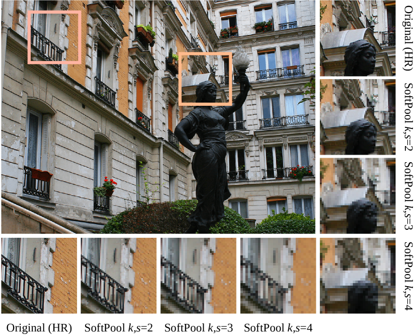
Figure 6: Results after SoftPool pooling with different kernel and stride sizes. Image (img003) is from Urban100 [17].

To test the computation and memory overhead, we report running-time memory use and inference on both CPU and GPU (CUDA) in Table 3. We detail our testing environment and implementation in §7 of the Supplementary Material.

From Table 3 we observe that our implementation of SoftPool achieves low inference times for both CPU- and CUDA-based operations, while remaining memory-efficient. This is because the method allows parallelization and is simple to compute within a region. SoftPool is second only to average pooling in terms of latency and memory use as operations can be performed in-place at the tensor.

4.4 Classification performance on ImageNet1K

We investigate whether classification accuracy improves as a result of SoftPool’s superior ability to retain information. We replace the original pooling layers in ResNet [15], DenseNet [16], ResNeXt [41] and wide-ResNet [44] networks. These models were chosen because of their wide use. We consider two distinct settings. In the from scratch setting, we replace the pooling operators of the original models by SoftPool and train with weights randomly initialized. In the pre-trained setting, we replace pooling layers of the original trained networks and evaluate the effects of the layer change on the ImageNet1K validation set without further training. Results of both settings appear in Table 2.

Networks trained from scratch with pooling layers replaced by SoftPool yield consistent accuracy improvements over the original networks. The same trend is also visible for the pre-trained networks for which the models have been trained with their original pooling methods. We now discuss the results per CNN architecture family.

ResNet [15]. By training from scratch with SoftPool, an average top-1 accuracy improvement of 1.17% is observed with a maximum of 1.51% on ResNet18. When replacing pooling layers on pre-trained networks, we obtain an average of +0.59% accuracy. All ResNet-based models only include a single pooling operation after the first convolution. Thus, results are based on a single layer replacement which emphasizes the merits of using SoftPool.

Model	pooling replacement	statistic ($\chi^{2}$)	p-value ($\rho$)
ResNet18	Max $\rightarrow$ SoftPool	$90.08$	$2.28e^{-21}$
ResNet34		$15.04$	$1.05e^{-4}$
ResNet50		$61.80$	$3.80e^{-15}$
ResNet101		$23.13$	$1.51e^{-6}$
ResNet152		$50.29$	$1.32e^{-12}$
DenseNet121	Avg+Max $\rightarrow$ SoftPool	$411.02$	$2.19^{-91}$
DenseNet161		$46.52$	$9.06e^{-12}$
DenseNet169		$27.32$	$1.72e^{-7}$
ResNeXt50 32x4d	Max $\rightarrow$ SoftPool	$45.13$	$1.85e^{-11}$
ResNeXt101 32x8d		$695.87$	$2.36e^{-53}$
wide-ResNet50	Max $\rightarrow$ SoftPool	$39.41$	$3.43e^{-10}$
InceptionV1	Max $\rightarrow$ SoftPool	$106.41$	$5.98e^{-25}$
InceptionV3		$80.19$	$3.39e^{-19}$

Table 4: McNemar’s [9, 24] statistical significance for pooling substitution results correlation. The top-1 accuracies on ImageNet1K val set from Tables 2, 5 and 6 are used. A detailed view of the statistics is presented in §6 in the Supplementary Material.

DenseNet [16]. Based on the DenseNet overall architecture that incorporates five pooling operations, we replace the max pooling operation that follows after the first layer and average pooling layers between Dense blocks with our proposed method. Top-1 accuracy gains are in the 0.93–1.23% range when training from scratch and 0.47–0.57% with substitution on pre-trained networks. The top-5 accuracy follows similar incremental trends. The largest increment in both settings is observed for DenseNet121.

ResNeXt [41]. Average of 0.83% top-1 accuracy improvement when trained from scratch. The best model, ResNeXt101 32x8d, achieves 80.12% top-1 accuracy (+0.81%) and 94.88% top-5 accuracy (+0.60%) with SoftPool. On the pre-trained settings, we note average improvements of +0.59% on top-1 and +0.36% top-5 accuracies. We again note these accuracies come by a replacement of their only pooling operation after the first convolution layer and without additional training.

Wide-Resnet-50 [44]. We observe top-1 and top-5 accuracy increases of 1.01% and 0.76% when trained from scratch with SoftPool. The initialized network also achieves improvements with +0.63% top-1 and +0.42% top-5.

Pooling	Networks
	ResNet18 [15]	ResNet34 [15]	ResNet50 [15]	ResNeXt50 [41]	DenseNet121 [16]	InceptionV1 [34]
Original	(Max)	(Max)	(Max)	(Max)	(Avg+Max)	(Max)
	69.76	73.30	76.15	77.62	74.65	69.78
Stochastic [45]	70.13	73.34	76.11	77.71	74.84	70.14
S3 [46]	70.15	73.56	76.24	77.82	74.85	70.17
$L_{p}$ [22]	70.45	73.74	76.56	77.86	74.93	70.32
Gate [14]	70.74	73.68	76.75	77.98	74.88	70.52
DPP [28]	70.86	74.25	77.09	78.20	75.37	70.95
LIP [12]	70.83	73.95	77.13	78.14	75.31	70.77
SoftPool (ours)	71.27	74.67	77.35	78.48	75.88	71.43

Table 5: Pooling layer substitution top-1 accuracy for a variety of pooling methods. Experiments were performed on Imagenet1K.

Layer	Pooling layer substitution with SoftPool
	N	I	II	III	IV	V	VI	VII
$pool_{1}$		✓	✓	✓	✓	✓	✓	✓
$pool_{2}$			✓	✓	✓	✓	✓	✓
$mixed\;5_{b-d}$				✓	✓	✓	✓	✓
$mixed\;6_{a}$					✓	✓	✓	✓
$mixed\;6_{b-e}$						✓	✓	✓
$mixed\;7_{a}$							✓	✓
$mixed\;7_{b-d}$								✓
Top-1 (%)	77.45	77.93	78.14	78.37	78.42	78.65	78.83	79.04
Top-5 (%)	93.56	93.61	93.68	93.74	93.78	93.84	93.90	93.98

Table 6: Progressive layer substitution for InceptionV3. Experiments are performed on ImageNet1K. Column numbers refer to the number of replaced pooling layers, marked with ✓.

[t] Model GFLOPs HACS Kinetics-700 UCF-101 top-1(%) top-5(%) top-1(%) top-5(%) top-1(%) top-5(%) r3d-50 [18]^∗∗ 53.16 78.36 93.76 49.08 72.54 93.13 96.29 r3d-101 [18]^∗∗ 78.52 80.49 95.18 52.58 74.63 95.76 98.42 r(2+1)d-50 [37]^∗∗ 50.04 81.34 94.51 49.93 73.40 93.92 97.84 I3D [4]^‡∗ 55.27 79.95 94.48 53.01 69.19 92.45 97.62 ir-CSN-101 [36]^‡† 17.26 N/A N/A 54.66 73.78 95.13 97.85 MF-Net [5]^†∗ 22.50 78.31 94.62 54.25 73.38 93.86 98.37 SlowFast r3d-50 [11]^‡† 36.71 N/A N/A 56.17 75.57 94.62 98.75 SRTG r3d-50 [33]^†† 53.22 80.36 95.55 53.52 74.17 96.85 98.26 SRTG r(2+1)d-50 [33]^†† 50.10 83.77 96.56 54.17 74.62 95.99 98.20 SRTG r3d-101 [33]^†† 78.66 81.66 96.37 56.46 76.82 97.32 99.56 r3d-50 with SoftPool (Ours) 53.16 79.82 94.64 50.36 73.72 93.90 97.02 SRTG r(2+1)d-50 with SoftPool (Ours) 50.10 84.78 97.72 55.27 75.44 96.46 98.73 SRTG r3d-101 with SoftPool (Ours) 78.66 83.28 97.04 57.76 77.84 98.06 99.82

• re-implemented models trained from scratch. $\dagger\dagger$ models and weights from official repositories. $\ddagger*$ unofficial models trained from scratch.

• models from unofficial repositories with official weights. $\dagger*$ official models trained from scratch.

Table 7: Action recognition top-1 and top-5 accuracy for HACS, Kinetics-700 and UCF-101. Models are trained on HACS and fine-tuned for Kinetics-700 and UCF-101, except for ir-CSN-101 and SlowFast r3d-50 (see text). N/A means no trained model was provided.

These combined experiments demonstrate that by replacing a single pooling layer (ResNet, ResNeXt and Wide-ResNet) or only five pooling layers (DenseNet) with SoftPool operations leads to a modest but important increase in accuracy. To understand whether these improvements are statistically significant, we performed a McNemar’s test [9, 24] to calculate the probabilities ($\rho$) of marginal homogeneity between the original and the SoftPool-replaced networks. The results are summarized in Table 4 for the models obtained in the from scratch setting. As shown for all networks, $\rho\!\ll\!0.01$ which corresponds to confidence $\gg\!99\%$ that the improved results are indeed due to the different pooling operations.

Memory and computation requirements. We also summarize the number of parameters and GLOPs in Table 2. SoftPool does not include trainable variables and thus does not affect the number of parameters, in contrast to recent pooling methods [12, 14, 19, 28]. We also depart from these methods as the number of GFLOPs remains the same as the maximum and average pooling that we replace.

Pooling method comparisons. In Table 5, we compare multiple pooling methods across six networks. All networks were trained from scratch. SoftPool performs similarly to learnable approaches without requiring additional convolutions, while outperforming stochastic methods. These classification accuracies correlate with image similarities in Table 1. This enforces the notion that pooling methods that retain information will also improve classification accuracy.

4.5 Multi-layer ablation study

In order to better understand how SoftPool affects the network performance at different depths, we use an InceptionV3 model [35] which integrates pooling in its layer structure. We systematically replace the max-pool operations within Inception blocks at different network layers.

From the top-1 and top-5 results summarized in Table 6, we observe that the accuracy increases with the number of pooling layers that are replaced with SoftPool. An average increase of 0.23% in top-1 accuracy is obtained with single layer replacements. The final top-1 accuracy surge between the original network with max-pool (N) and the SoftPool model (VII) is +1.59%. This shows that SoftPool can be used as direct replacement regardless of the network depth.

4.6 Classification performance on video data

Finally, we demonstrate the merits of SoftPool in handling spatio-temporal data. Specifically, we address action recognition in videos where the input to the network is a stack of subsequent video frames. Representing time-based features stands as a major challenge in action recognition research [32]. The main challenge in space-time data downsampling is the inclusion of key temporal information without impacting the spatial quality of the input.

In this experiment, we use popular time-inclusive networks and replace the original pooling methods with SoftPool. Most space-time networks extend 2D convolutions to 3D to account for the temporal dimension. They use stacks of frames as inputs. For the tested networks with SoftPool, the only modification is that we use SoftPool to deal with the additional input dimension (see Section 3.4).

We trained most architectures from scratch on HACS [47] using the implementations provided by the authors. Results for Kinetics-700 and UCF-101 are fine-tuned from the HACS-trained models. We make exceptions for ir-CSN-101 and SlowFast, for which we used the networks trained for Kinetics-700 that were provided by the authors. ir-CSN-101 [36] is pre-trained on IG65M [13], a large dataset consisting of 65M video that is not publicly available. SlowFast [11] is pre-trained on the full ImageNet dataset.

Results appear in Table 7. For three architectures, we report the performance on both the vanilla models and their counterparts with all pooling operations replaced by SoftPool. For r3d-50, a ResNet with 3D convolutions, using SoftPool increases the top-1 classification accuracy by 1.46%. The accuracy performance also increases with 1.00% and 1.63% for the two SRTG models [33]. For the SRTG model with ResNet-(2+1) backbone, we achieve state-of-the-art performance on HACS. Also when using spatio-temporal data, SoftPool does not add computational complexity (GFLOPS), as demonstrated in Table 7.

For the performance on Kinetics-700, we observe important performance gains. An average of 1.22% increase in top-1 accuracy is shown for the three models that have their pooling operations substituted by SoftPool. The best performing model is SRTG r3d-101 with SoftPool, which achieves a top-1 accuracy of 57.76% and a top-5 accuracy score 77.84%. These models also outperform state-of-the-art models such as SlowFast r3d-50 and ir-CSN-101.

When fine-tuning on UCF-101, the average accuracy gain is 0.66% despite an almost saturated performance. SRTG r3d-101 with SoftPool is the best performing model with a top-1 accuracy of 98.06% and top-5 of 99.82%.

5 Conclusions

We have introduced SoftPool, a novel pooling method that can better preserve informative features and, consequently, improves classification performance in CNNs. SoftPool uses the softmax of inputs within a kernel region where each of the activations has a proportional effect on the output. Activation gradients are relative to the weights assigned to them. Our operation is differentiable, which benefits efficient training. SoftPool does not require additional parameters nor increases the number of performed operations. We have shown the merits of the proposed approach through experimentation on image similarity tasks as well as on the classification of image and video datasets. We believe that the increase in classification performance combined with the low computation and memory requirements make SoftPool an excellent replacement for current pooling operations, including max and average pooling.

Refining activation downsampling with SoftPool – Supplementary material
      

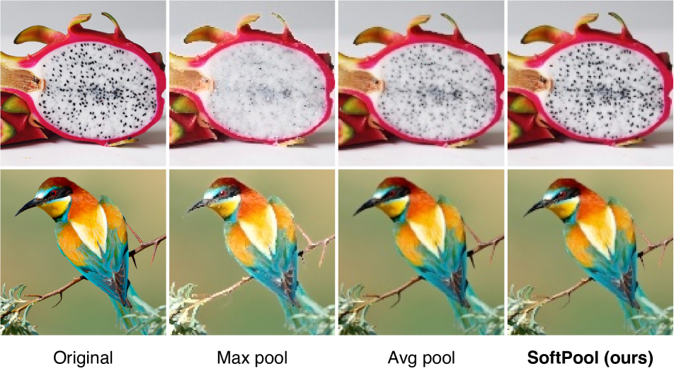
Figure S1-0: High resolution pooled images. Original images are of size $1200\times 1200$. The downsampled images were created with $\times 3$ pooling operations. To match the sizes of the original images and make the downsampling result more visible, we used inter area interpolation to resize the pooled images. This does not create a smoothing effect between neighboring pixels that are interpolated but rather populates new pixels based on the area relation.

S1-0 Detail preservation

We discussed and demonstrated the feature preservation capabilities of SoftPool in Section 3.3. Here, we provide high-resolution images from examples in Figure 3 of the paper, in order to demonstrate clearer the effects of each pooling method. As it can be seen in Figure Refining activation downsampling with SoftPool, SoftPool can better capture detail in high-contrasting areas. Evidence of this can be seen in the top image where the dragon fruit seeds are not always preserved in the down-sampled images. For max pooling, most of the seeds are lost. This also applies to a certain extent to average pooling. By selecting the average within a region, features with high contrast are smoothed over, which reduces their effect significantly. In contrast, SoftPool preserves such regions in the sub-sampled outputs. By including part of the low-intensity regions in the output while weighting the high-intensity regions more, it can preserve the little-contrasting pixels. A similar pattern can also be seen with low-contrasting regions such as the bird’s eye in the second row where, again, max pooling will highlight the high intensity features in the output while the downsampled output becomes less similar to that of the original image. Average pooling would instead make low-contrast features much more difficult to be recognized. SoftPool provides a balance between the two methods by weighting each part of the region respectfully to its intensity value.

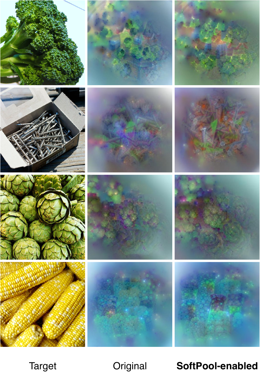
Figure S2-0: Neuron activation maximization for InceptionV3 with original and SoftPool pooling layers. We maximized the top-10 neurons erhan2009visualizing,stergiou2021mind of the final block (Mixed7c) in InceptionV3 [35]. Target top-10 neuron combinations for each row were selected for ImageNet1K classes “broccoli”, “nails”, “artichoke” and “corn”.

S2-0 Model feature visualization

Learned feature interpretability aims at understanding the features that networks associate with each class. One technique is activation maximization erhan2009visualizing which creates a synthetic image by maximizing the activations relating to a specific neuron. Neurons could correspond to a specific class simonyan2013deep or features within the feature extractor dosovitskiy2016inverting.

To test the representation capabilities of networks with SoftPool, we use InceptionV3 [35] as a backbone model and visualize the top-10 most informative features. To train, we initialize an image with random noise, which we use as input for each of the two tested networks. During the training process, the image is optimized with the maximization of the activations of the top-10 kernels in the final InceptionV3 block (Mixed7c) as objective function. The top-10 kernels are selected based on the highest average activations across all class examples. To eliminate additional noise, we use a mask-based approach similar to Wei et al. wei2015understanding. However, in our setting, the mask is responsible for reducing the size of the gradient vectors for regions that are further away from the image center.

We used input images of size $512\times 512$ in order to get higher-definition features. We use an SGD optimizer with an initial learning rate of 0.1 with a linear decrease to 0.01 over 2,000 total iterations. We use a weight decay of 1e-6. The weights for both models were initialized from those shown in Table 6 of the paper.

We show the outputs in Figure S2-0 for four ImageNet1K classes: “broccoli”, “nails”, “artichoke” and “corn”. We include in the left column the ImageNet1K images with the highest activations to provide representative examples. The majority of the features are fairly similar between the two models. Since SoftPool does not change the overall architecture nor the parameters, a high degree of similarity is expected. However, in cases such as the heads of the nails, we do notice a better definition of the objects. We also notice for the artichoke class that the structure of the petals and the thorns are more easy to distinguish from the network with SoftPool layers compared to the network with the original pooling layers. Although the differences remain small, by only changing the downsampling method used by the network, it can affect the robustness and improve the feature interpretability to a degree.

S3-0 Spatio-temporal volume pooling

Pooling operations in time-inclusive volumes (videos) face the additional challenge of encoding time in the output. One large problem is between-frame motion as it can significantly impact the representation of spatial features within frames in the sub-sampled volume.

We show in Figure S3-0 with four different examples the effects of spatio-temporal pooling with average pooling, max-pool, and SoftPool operations. As none of the methods is tailored towards completely alleviating the effects of encoded motion in the pooled output, they are visible in edges and regions where cross-frame motion exists. However, differences between the three methods become apparent.

Parkour

Running

Dodgeball

Table tennis

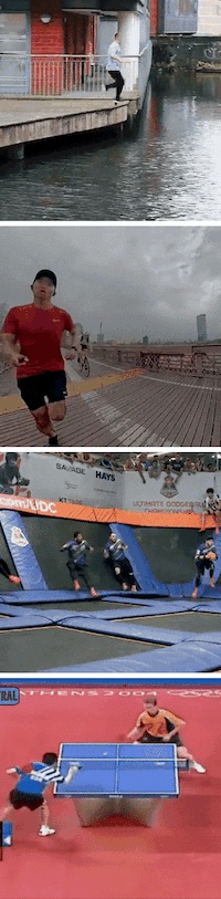
Figure S3-0: a. Original

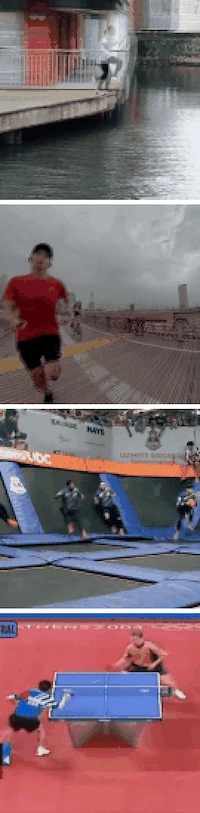
Figure S3-0: b. Avg. pool (3D)

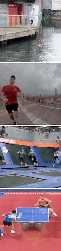
Figure S3-0: c. Max-pool (3D)

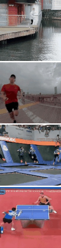
Figure S3-0: d. SoftPool (3D)

Figure S3-0: e. Zoomed-in frame regions

Figure S3-0: Spatio-temporally downsampled videos. Sub-sampling over spatio-temporal volumes compared to original videos (a), and downsampled with average pooling (b), maximum pooling (c) and our proposed SoftPool (d). Two zoomed-in frame regions appear in (e).

We demonstrate part of these differences in Figure S3-0(e). Where we include two cases of zoomed-in frame regions that show some variance based on the pooling method used. In the top one, gaps in the wooden planks of the floor are significantly less distinguishable within the max-pooled frame. Consequently, in the average pooled frame region, the nails are not visible at all anymore. This effect is in line with our observations for image-based downsampling of high-contrast and low-contrast regions. In contrast, SoftPool preserves features in both cases, which allows for the extraction of representative features after pooling.

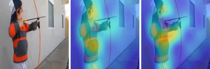
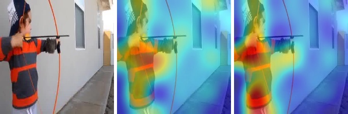
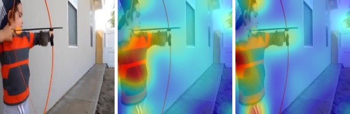
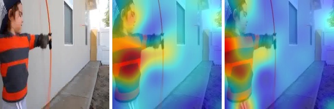
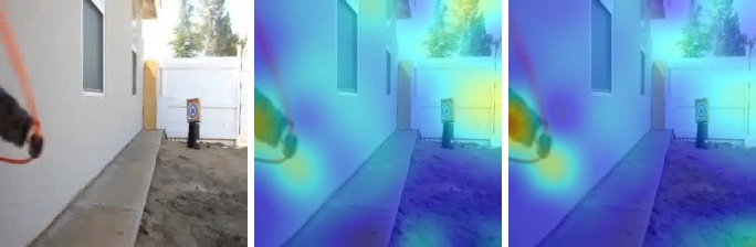
Source video           original             with SoftPool           Source video           original             with SoftPool

Figure S4-0: Spatio-temporal saliency region visualizations for r3d-50 with and without SoftPool. Class Feature Pyramids stergiou2019class,stergiou2019saliency were used to generate the regional activations in the final conv layer of r3d-50.

S4-0 Time-inclusive salient regions

To better understand the use of SoftPool in 3D-CNNs, we study the spatio-temporal regions that the network finds more informative. Similar to the activation maximization visualizations for images, we use a fixed network structure as a backbone and only study the variations produced by replacing the original pooling operations with SoftPool. For the visualizations in Figure S4-0, we use the r3d-50 network from Table 5 in the paper. The examples are sampled from the Kinetics-700 dataset from the classes “building lego” and “archery”.

Based on the examples presented in Figure S4-0, there are no significant differences in the salient regions. However, in multi-object scenes such as for the “building lego” class, the regional focus of the SoftPool network is shown to be a bit more distinct towards the region where there is a clear definition of the action performed (i.e. the hand with the lego brick). The case of “archery” exhibit small amounts of variations, with both either focusing on the main actor within the video.

S5-0 Embedding spaces visualizations

We provide t-SNE maaten2008visualizing visualizations of feature embeddings from an InceptionV3 model with original pooling operations and their counterparts with all pooling operations replaced by SoftPool. We use the averaged feature vectors of the final block in InceptionV3 (Mixed7c) with a reduced dimensionality of 50 channels produced by PCA jolliffe2003principal and then perform t-SNE. We further perform k-means clustering lloyd1982least to better represent the different sub-clusters within the embedding space. In well-defined feature spaces, images in clusters that are closer together should be more similar.

The visualizations in Figures S5-0-S7-0 show distinct embeddings for the two networks. While structurally both model yield similar embeddings, for some classes the differences are more apparent. For example, class “jack-o-lantern” (Figure S6-0) and “sax” (Figure S7-0) show more compact representations when SoftPool is used.

S6-0 Error rates and statistical significance

We further evaluate the statistical significance of the validation accuracy rates achieved in Table 2 in the context of the classification performance between the original models and models with pooling layers replaced by SoftPool. We perform a McNemar’s test [9, 24], which is based on a null hypothesis ($H_{0}$) corresponding to accuracy homogeneity between the two models. It is calculated based on a contingency table holding the number of correct or incorrect class prediction instances with respect to each model. The tests studies the number of disagreements in the predictions between the two models. The Chi-Square statistic ($\chi^{2}$) is then calculated based on the number of model $i$ correct predictions against model $j$ incorrect predictions ($n_{ij}$) and model $j$ correct against model $i$ incorrect predictions ($n_{ji}$). This is expressed as:

$$\chi^{2}=\frac{(|n_{ij}-n_{ji}|-1)^{2}}{n_{ij}+n_{ji}}$$ (S1)

We note that the null hypothesis ($H_{0}$) can be rejected with different significance levels based on the Chi-Square distribution table chidisttable. As the statistic is calculated with a single degree of freedom, $\chi^{2}$ values of $\{3.84,5.02,6.63\}$ correspond to equivalent probabilities of $\{95\%,97.5\%,99.0\%\}$ that the two methods indeed differ.

		Original		Total
		Correct	Incorrect
SoftPool	Correct	31838	3795	35633
	Incorrect	3011	11356	14367
Total		34849	15151	50000

(a) ResNet18

		Original		Total
		Correct	Incorrect
SoftPool	Correct	34090	3246	37336
	Incorrect	2940	9724	12664
Total		37030	12970	50000

(b) ResNet34

		Original		Total
		Correct	Incorrect
SoftPool	Correct	35472	3203	38675
	Incorrect	2603	8722	11325
Total		38075	11925	50000

(c) ResNet50

		Original		Total
		Correct	Incorrect
SoftPool	Correct	36553	2609	39162
	Incorrect	2272	8566	10838
Total		38825	11175	50000

(d) ResNet101

		Original		Total
		Correct	Incorrect
SoftPool	Correct	37247	2373	39620
	Incorrect	1908	8472	10380
Total		39155	10845	50000

(e) ResNet152

		Original		Total
		Correct	Incorrect
SoftPool	Correct	34097	3836	37933
	Incorrect	2253	9814	12067
Total		36350	13650	50000

(f) DenseNet121

		Original		Total
		Correct	Incorrect
SoftPool	Correct	35160	4237	39397
	Incorrect	3631	6972	10603
Total		38791	11209	50000

(g) DenseNet161

		Original		Total
		Correct	Incorrect
SoftPool	Correct	35074	3407	38481
	Incorrect	2988	8531	11519
Total		38062	11938	50000

(h) DenseNet169

		Original		Total
		Correct	Incorrect
SoftPool	Correct	36628	2618	39246
	Incorrect	2153	8601	10754
Total		38781	11219	50000

(i) ResNeXt50

		Original		Total
		Correct	Incorrect
SoftPool	Correct	38633	2587	41220
	Incorrect	1005	7775	8780
Total		39638	10362	50000

(j) ResNeXt101

		Original		Total
		Correct	Incorrect
SoftPool	Correct	36638	3113	39751
	Incorrect	2636	7613	10249
Total		38781	10726	50000

(k) wide-ResNet50

		Original		Total
		Correct	Incorrect
SoftPool	Correct	31826	3897	35723
	Incorrect	3037	11240	14277
Total		34863	15137	50000

(l) InceptionV1

		Original		Total
		Correct	Incorrect
SoftPool	Correct	36341	3029	14874
	Incorrect	2370	8260	10630
Total		38711	11289	50000

(m) InceptionV3

Table S1: Error summaries of original models and models with pooling replaced with SoftPool.

Prediction distributions of each model pair are presented in Table S1 and the resulting $\chi^{2}$ statistics and $\rho$ homogeneity probabilities are presented in Table 4 in the main text. Based on the very low homogeneity probability $\ll 0.01\%$ craparo2007significance,fisher1992statistical,neyman1937outline, the differences between the original networks and the networks that have been re-trained with SoftPool cannot be attributed to statistical errors.

S7-0 Implementation Details

Range definitions. The exponential weighting of activations can correspond to the produced values being smaller than the type’s (16, 32, 64-bit) precision level lower threshold. This can either result in a computational underflow or in a zero-valued dividend. For this reason, we include additional checks that each produced exponentially scaled activation $e^{\textbf{a}_{i}}$ and their resulting weight mask $\textbf{w}_{i}$, based on which their values ($x$) are transformed, to $x=max(0,x)$. The sum of the weights is constrained similarly, based on $x=max(x_{min},x)$, where $x_{min}$ is the lowest limit based on type chosen to ensure non-zero dividend. We note that these checks do need to address changes in the activation functions used. The current tested networks use ReLU activations which have lower bounds of zero. When considering other non-zero or negative-valued lower bound functions, the transformations need to be adjusted accordingly.

Computational description. As our implementation is native to CUDA-enabled devices, we are able to achieve inference times close to those of native methods such as average and maximum pooling. However, the parallelization capabilities of SoftPool allow for running times similar to those of average pooling with $O(1)$. This is based on the fact that operations can be performed through a matrix over the kernel region. This is beneficial for processes that have parallelization as a backbone (CUDA). In contrast, max pooling has complexity of at least $O(n)$, as the selection of the maximum value within the region can only be performed through the sequential consideration of each pixel within the region.

Testing environment. All of our tests were done with half floating point precision (float16) instead of single-point (float32) for better memory utilization during the model training phase. The batch sizes are split equally with 64 images per GPU. Our testing environment consists of an AMD Threadripper 2950X with 2400MHz RAM frequency and four Nvidia 2080 TIs.

plain egbib

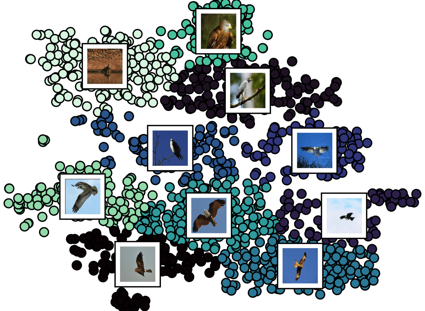
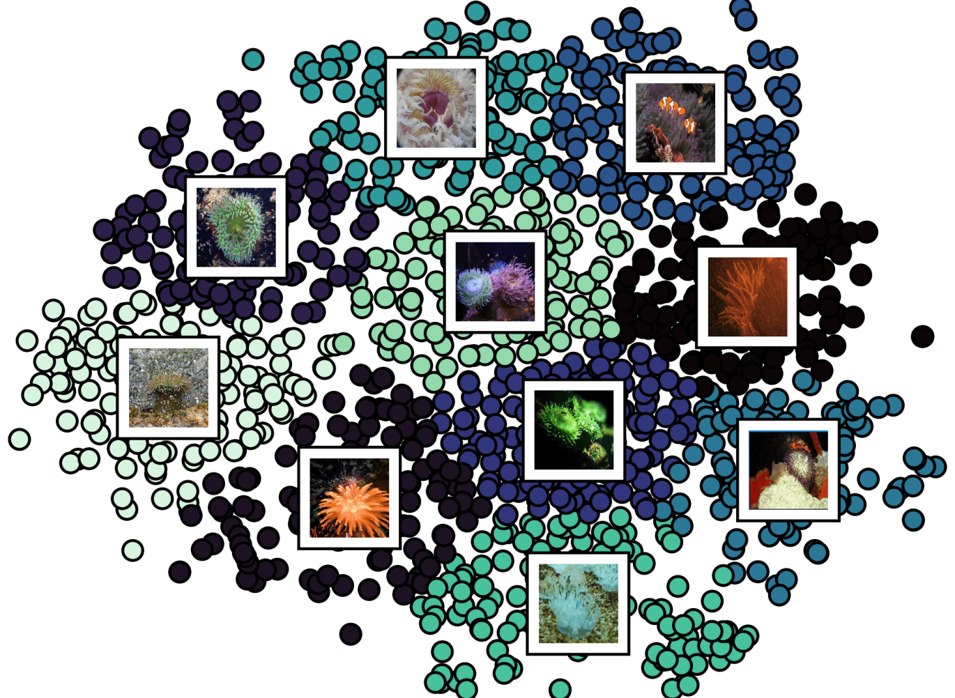
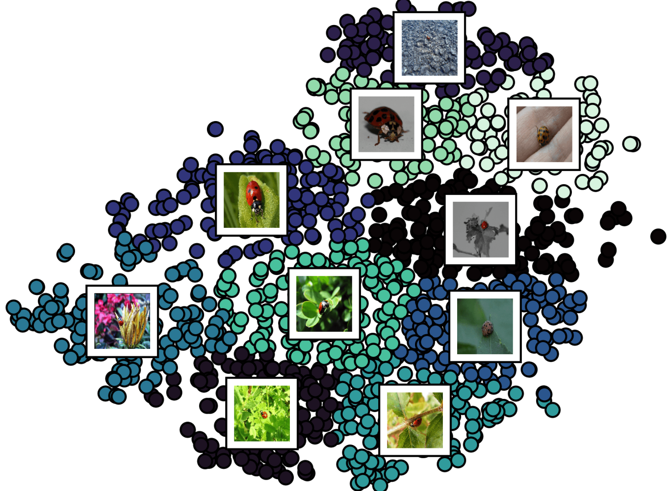
Figure S5-0: a. Original

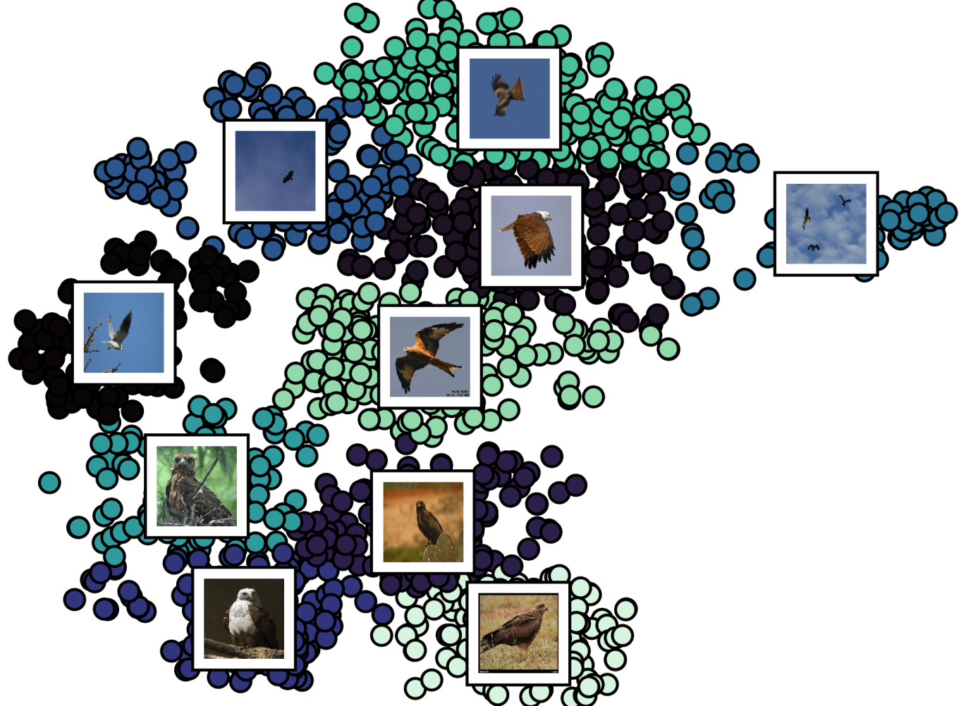
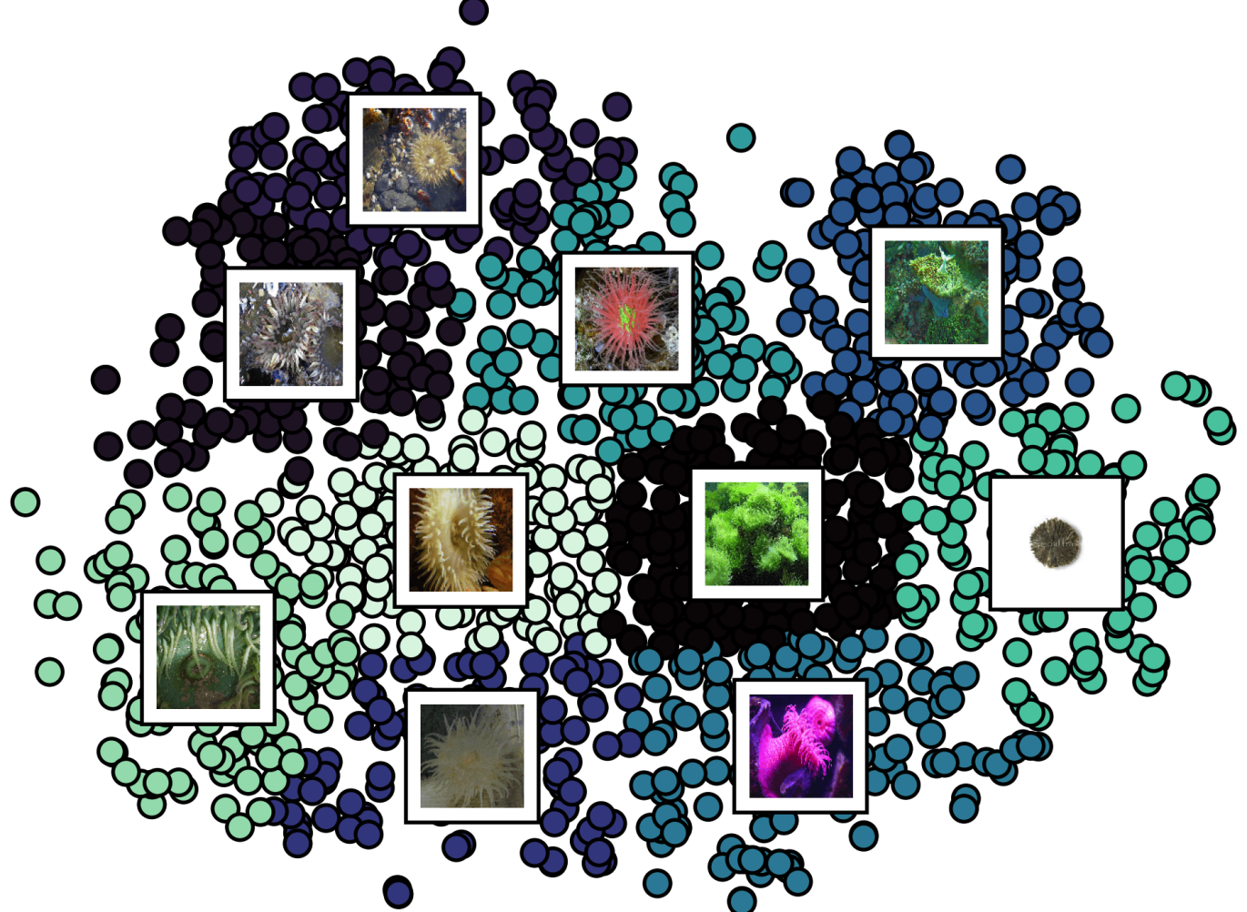
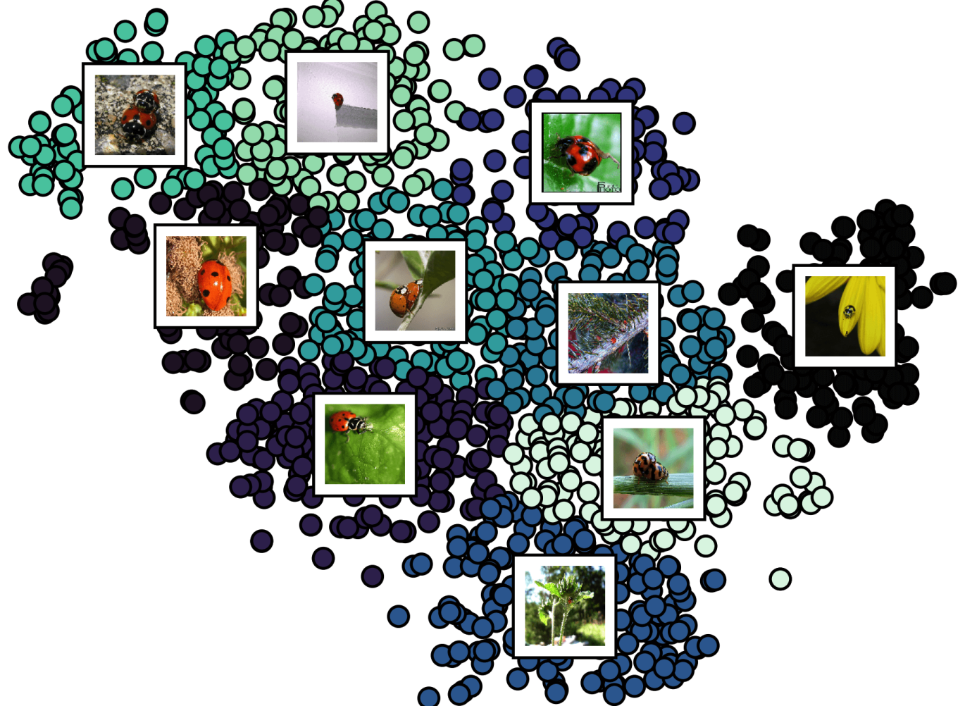
Figure S6-0: b. SoftPool

Figure S5-0: t-SNE feature embeddings for InceptionV3 with and without SoftPool. ImageNet1K classes “bald eagle”, “sea anemone” and “ladybug”. Cluster centers are found with k-means to better visualize the feature space. Images displayed are the closest examples for each cluster center.

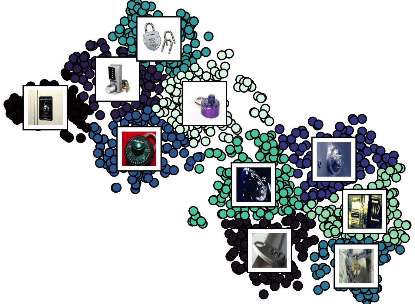
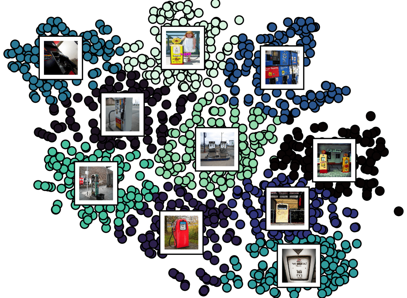
Figure S6-0: a. Original

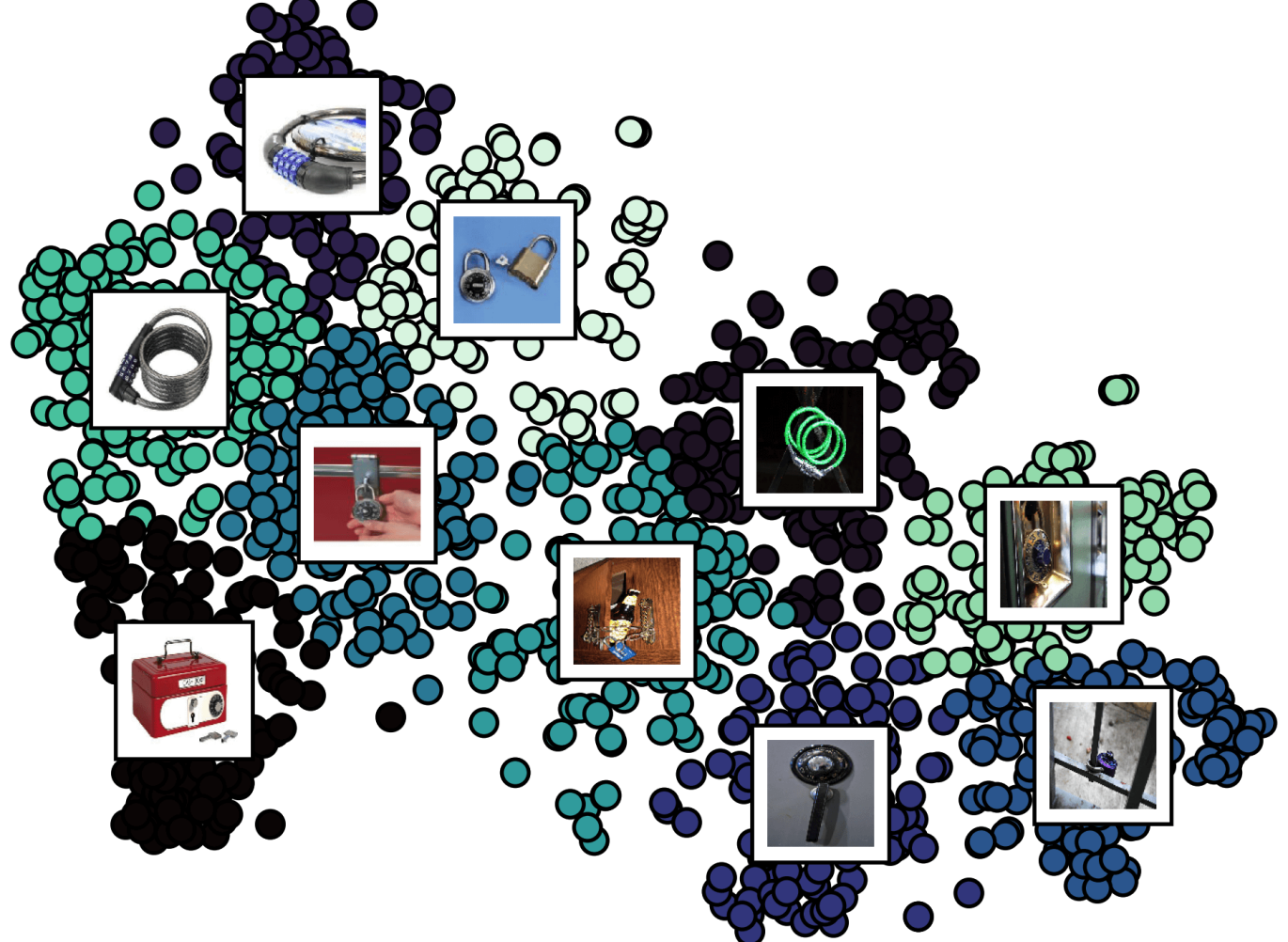
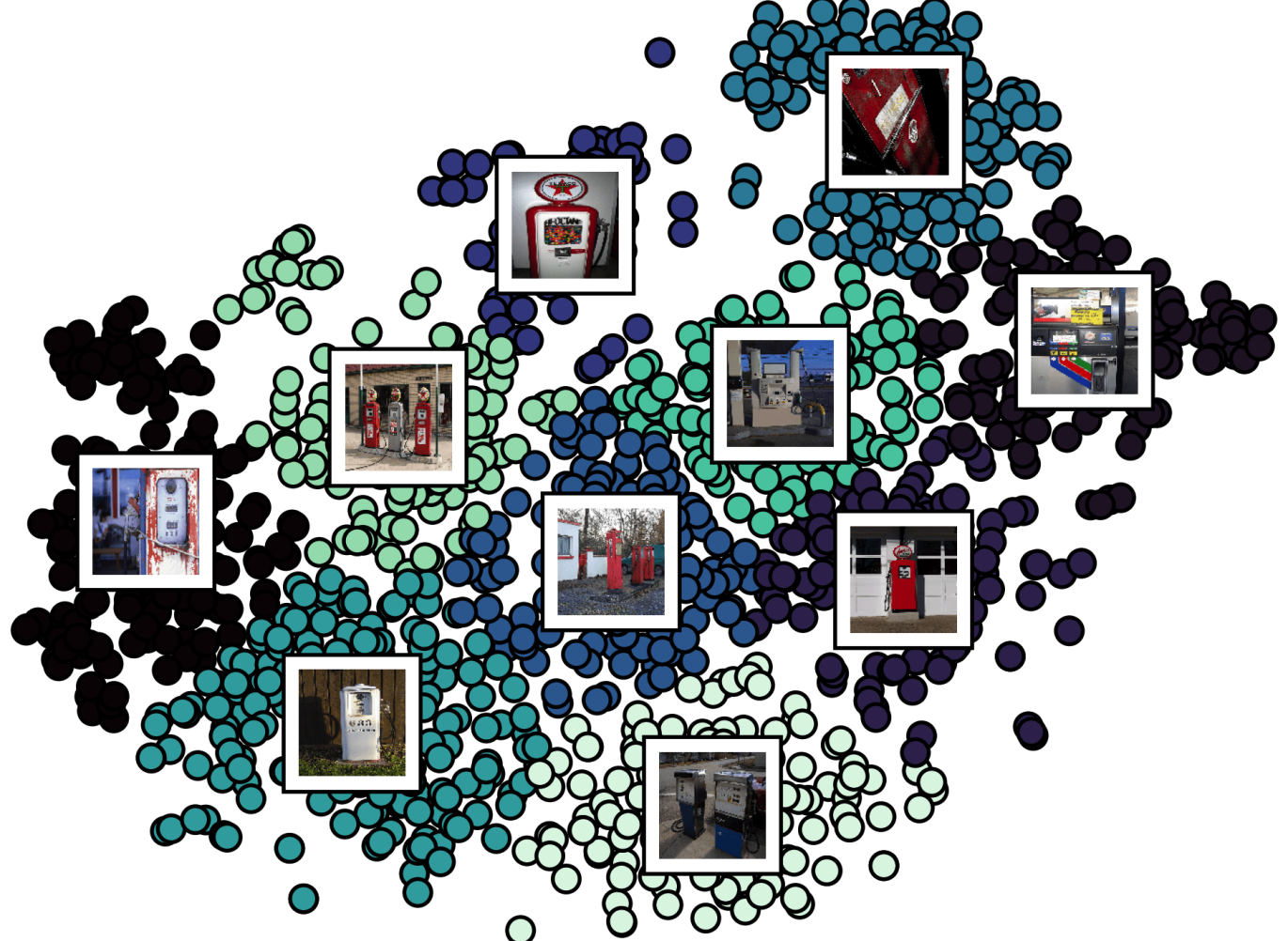
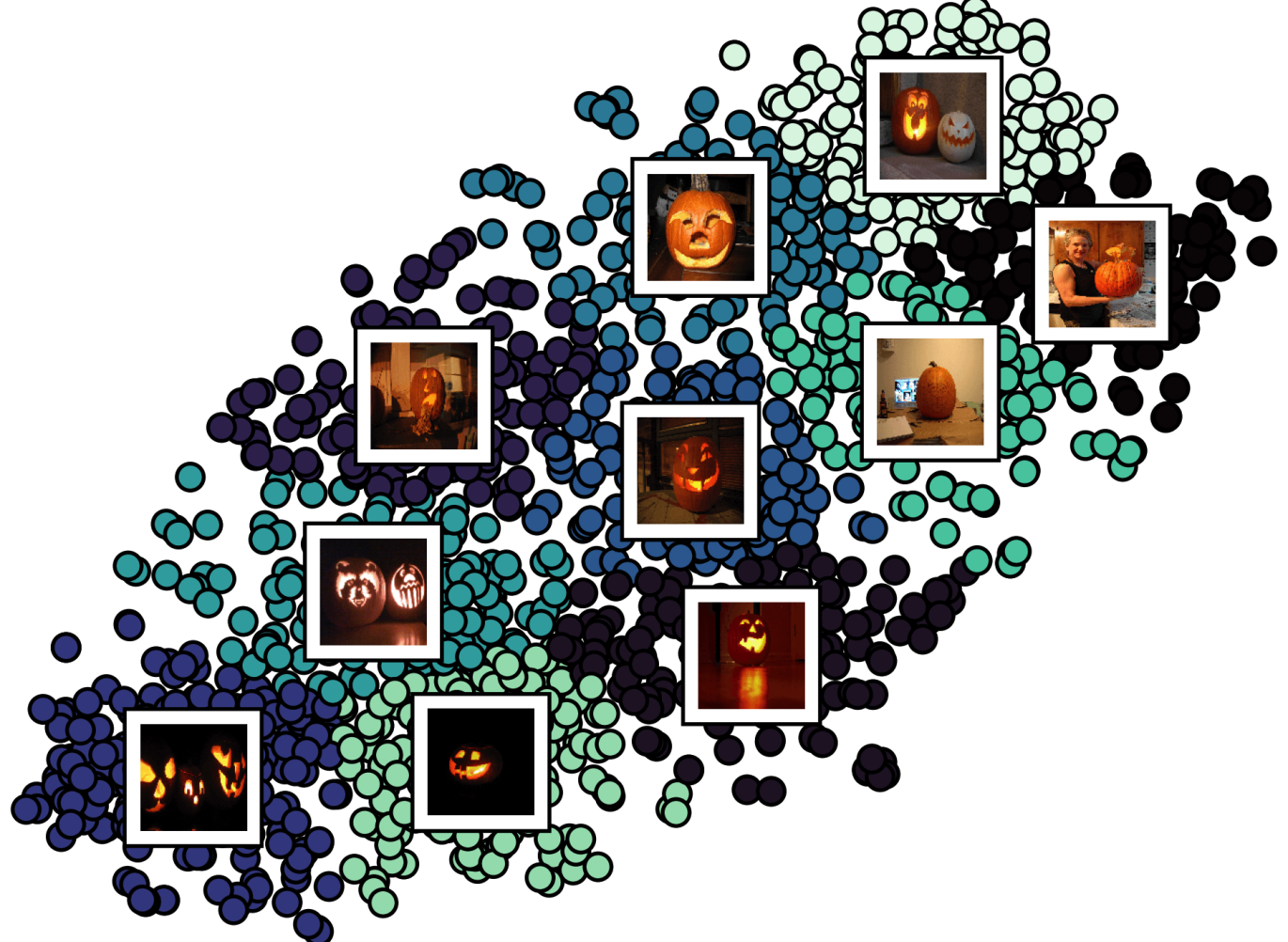
Figure S7-0: b. SoftPool

Figure S6-0: t-SNE feature embeddings for InceptionV3 with and without SoftPool. ImageNet1K classes “combination lock”, “gas pump” and “jack-o-lantern”. Cluster centers are found with k-means to better visualize the feature space. Images displayed are the closest examples for each cluster center.

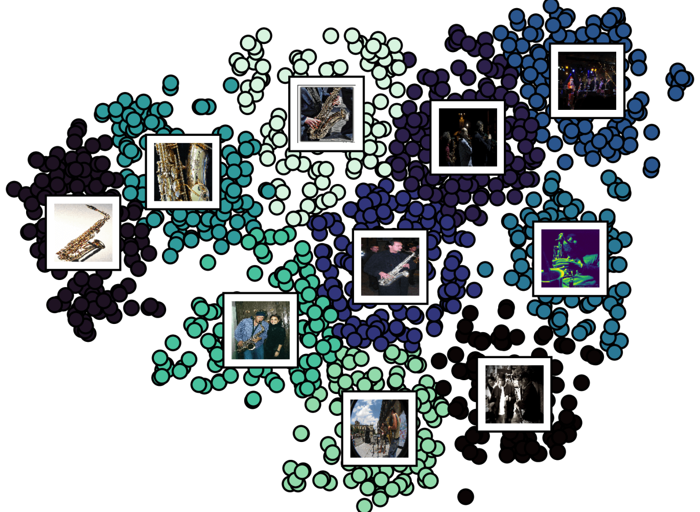
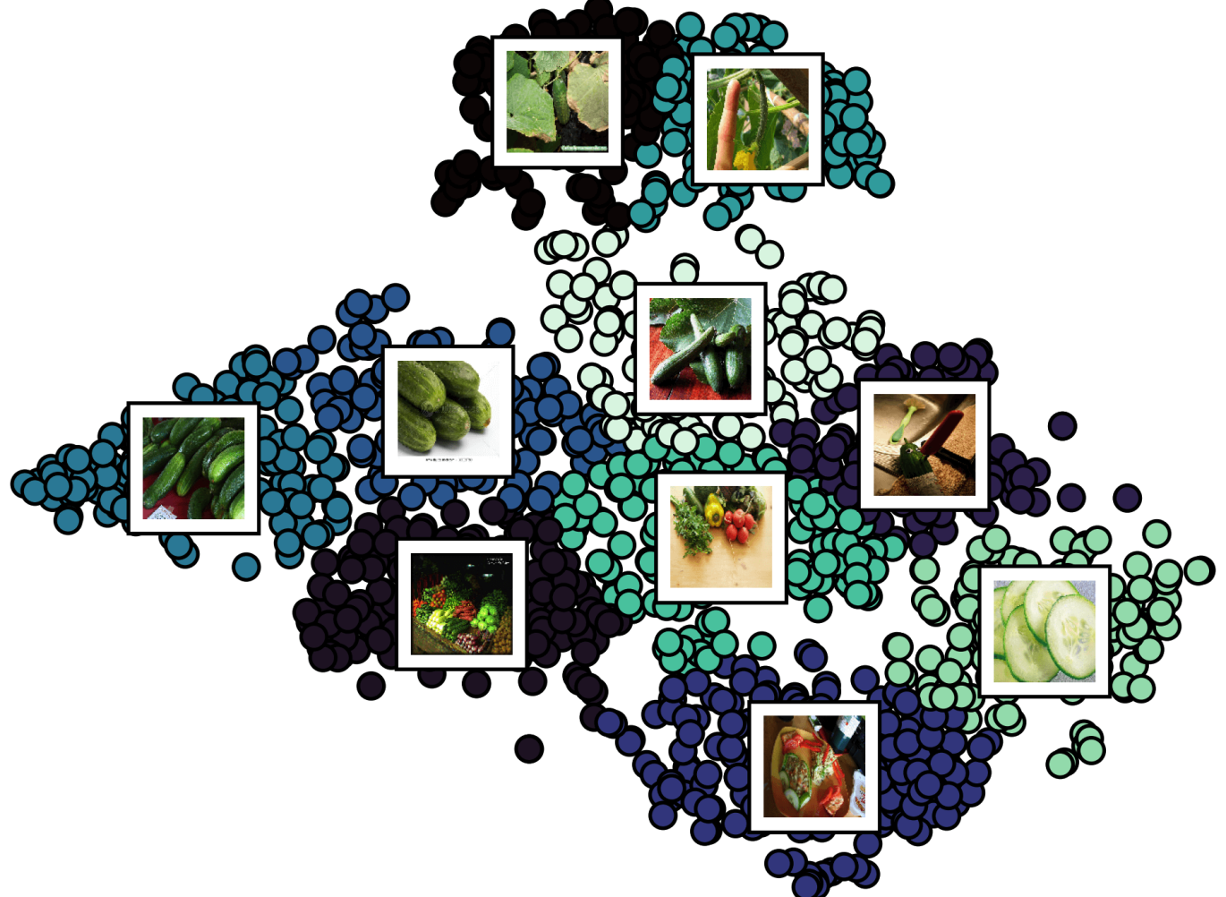
Figure S7-0: a. Original

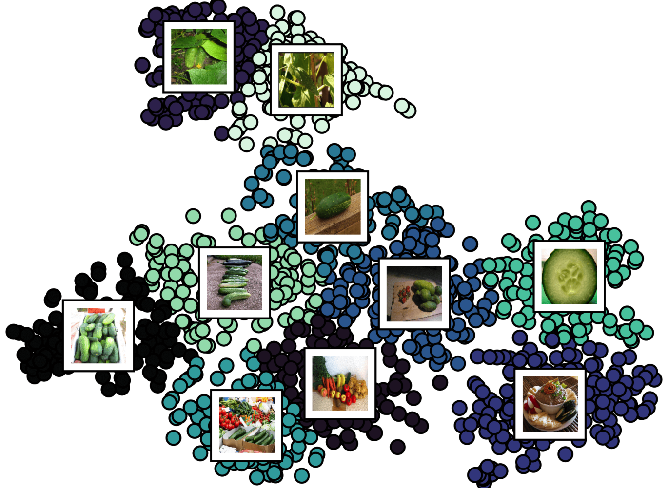
Figure S8-0: b. SoftPool

Figure S7-0: t-SNE feature embeddings for InceptionV3 with and without SoftPool. ImageNet1K classes “sax” and “zucchini”. Cluster centers are found with k-means to better visualize the feature space. Images displayed are the closest examples for each cluster center.

References

- [1] Eirikur Agustsson and Radu Timofte. Ntire 2017 challenge on single image super-resolution: Dataset and study. In Conference on Computer Vision and Pattern Recognition Workshops (CVPRW), pages 126–135, 2017.
- [2] Y-Lan Boureau, Jean Ponce, and Yann LeCun. A theoretical analysis of feature pooling in visual recognition. In International Conference on Machine Learning (ICML), pages 111–118, 2010.
- [3] Joao Carreira, Eric Noland, Chloe Hillier, and Andrew Zisserman. A short note on the Kinetics-700 human action dataset. arXiv preprint arXiv:1907.06987, 2019.
- [4] Joao Carreira and Andrew Zisserman. Quo vadis, action recognition? A new model and the Kinetics dataset. In Computer Vision and Pattern Recognition (CVPR), pages 4724–4733. IEEE, 2017.
- [5] Yunpeng Chen, Yannis Kalantidis, Jianshu Li, Shuicheng Yan, and Jiashi Feng. Multi-fiber networks for video recognition. In European Conference on Computer Vision (ECCV), pages 352–367, 2018.
- [6] Yunpeng Chen, Jianan Li, Huaxin Xiao, Xiaojie Jin, Shuicheng Yan, and Jiashi Feng. Dual path networks. In Advances in neural information processing systems (NeurIPS), pages 4467–4475, 2017.
- [7] Gabriella Csurka, Christopher Dance, Lixin Fan, Jutta Willamowski, and Cédric Bray. Visual categorization with bags of keypoints. In European Conference on Computer Vision Workshops (ECCVW), pages 1–22, 2004.
- [8] Adrien Deliège, Maxime Istasse, Ashwani Kumar, Christophe De Vleeschouwer, and Marc Van Droogenbroeck. Ordinal pooling. In British Machine Vision Conference, 2019.
- [9] Allen L Edwards. Note on the “correction for continuity” in testing the significance of the difference between correlated proportions. Psychometrika, 13(3):185–187, 1948.
- [10] Joan Bruna Estrach, Arthur Szlam, and Yann LeCun. Signal recovery from pooling representations. In International Conference on Machine Learning (ICML), pages 307–315. PMLR, 2014.
- [11] Christoph Feichtenhofer, Haoqi Fan, Jitendra Malik, and Kaiming He. SlowFast networks for video recognition. In International Conference on Computer Vision (ICCV), pages 6202–6211. IEEE, 2019.
- [12] Ziteng Gao, Limin Wang, and Gangshan Wu. Lip: Local importance-based pooling. In International Conference on Computer Vision (ICCV). IEEE, October 2019.
- [13] Deepti Ghadiyaram, Du Tran, and Dhruv Mahajan. Large-scale weakly-supervised pre-training for video action recognition. In Conference on Computer Vision and Pattern Recognition (CVPR). IEEE, 2019.
- [14] Caglar Gulcehre, Kyunghyun Cho, Razvan Pascanu, and Yoshua Bengio. Learned-norm pooling for deep feedforward and recurrent neural networks. In European Conference on Machine Learning and Knowledge Discovery in Databases (ECML PKDD), pages 530–546. Springer, 2014.
- [15] Kaiming He, Xiangyu Zhang, Shaoqing Ren, and Jian Sun. Deep residual learning for image recognition. In Computer Vision and Pattern Recognition (CVPR), pages 770–778. IEEE, 2016.
- [16] Gao Huang, Zhuang Liu, Laurens Van Der Maaten, and Kilian Q Weinberger. Densely connected convolutional networks. In Computer Vision and Pattern Recognition (CVPR), pages 2261–2269. IEEE, 2017.
- [17] Jia-Bin Huang, Abhishek Singh, and Narendra Ahuja. Single image super-resolution from transformed self-exemplars. In Conference on Computer Vision and Pattern Recognition (CVPR), pages 5197–5206, 2015.
- [18] Hirokatsu Kataoka, Tenga Wakamiya, Kensho Hara, and Yutaka Satoh. Would mega-scale datasets further enhance spatiotemporal 3d cnns? arXiv preprint arXiv:2004.04968, 2020.
- [19] Takumi Kobayashi. Global feature guided local pooling. In International Conference on Computer Vision (ICCV), pages 3365–3374. IEEE, 2019.
- [20] Svetlana Lazebnik, Cordelia Schmid, and Jean Ponce. Beyond bags of features: Spatial pyramid matching for recognizing natural scene categories. In Computer Vision and Pattern Recognition (CVPR), volume 2, pages 2169–2178. IEEE, 2006.
- [21] Yann LeCun, Léon Bottou, Yoshua Bengio, and Patrick Haffner. Gradient-based learning applied to document recognition. Proceedings of the IEEE, 86(11):2278–2324, 1998.
- [22] Chen-Yu Lee, Patrick W Gallagher, and Zhuowen Tu. Generalizing pooling functions in convolutional neural networks: Mixed, gated, and tree. In Artificial intelligence and statistics, pages 464–472, 2016.
- [23] Yusuke Matsui, Kota Ito, Yuji Aramaki, Azuma Fujimoto, Toru Ogawa, Toshihiko Yamasaki, and Kiyoharu Aizawa. Sketch-based manga retrieval using manga109 dataset. Multimedia Tools and Applications, 76(20):21811–21838, 2017.
- [24] Quinn McNemar. Note on the sampling error of the difference between correlated proportions or percentages. Psychometrika, 12(2):153–157, 1947.
- [25] Esteban Real, Alok Aggarwal, Yanping Huang, and Quoc V Le. Regularized evolution for image classifier architecture search. In Conference on Artificial Intelligence (AAAI), pages 4780–4789. AAAI, 2019.
- [26] Maximilian Riesenhuber and Tomaso Poggio. Hierarchical models of object recognition in cortex. Nature neuroscience, 2(11):1019–1025, 1999.
- [27] Olga Russakovsky, Jia Deng, Hao Su, Jonathan Krause, Sanjeev Satheesh, Sean Ma, Zhiheng Huang, Andrej Karpathy, Aditya Khosla, Michael Bernstein, Alexander C. Berg, and Li Fei-Fei. ImageNet Large Scale Visual Recognition Challenge. International Journal of Computer Vision (IJCV), 115(3):211–252, 2015.
- [28] Faraz Saeedan, Nicolas Weber, Michael Goesele, and Stefan Roth. Detail-preserving pooling in deep networks. In Conference on Computer Vision and Pattern Recognition (CVPR), pages 9108–9116. IEEE, 2018.
- [29] Thomas Serre, Lior Wolf, and Tomaso Poggio. Object recognition with features inspired by visual cortex. In Conference on Computer Vision and Pattern Recognition (CVPR), volume 2, pages 994–1000. IEEE, 2005.
- [30] Karen Simonyan and Andrew Zisserman. Very deep convolutional networks for large-scale image recognition. arXiv preprint arXiv:1409.1556, 2014.
- [31] Khurram Soomro, Amir Roshan Zamir, and Mubarak Shah. UCF101: A dataset of 101 human actions classes from videos in the wild. arXiv preprint arXiv:1212.0402, 2012.
- [32] Alexandros Stergiou and Ronald Poppe. Analyzing human-human interactions: A survey. Computer Vision and Image Understanding, 188:102799, 2019.
- [33] Alexandros Stergiou and Ronald Poppe. Learn to cycle: Time-consistent feature discovery for action recognition. Pattern Recognition Letters, 141:1–7, 2021.
- [34] Christian Szegedy, Wei Liu, Yangqing Jia, Pierre Sermanet, Scott Reed, Dragomir Anguelov, Dumitru Erhan, Vincent Vanhoucke, and Andrew Rabinovich. Going deeper with convolutions. In Computer Vision and Pattern Recognition, (CVPR). IEEE, 2015.
- [35] Christian Szegedy, Vincent Vanhoucke, Sergey Ioffe, Jon Shlens, and Zbigniew Wojna. Rethinking the inception architecture for computer vision. In Conference on Computer Vision and Pattern Recognition (CVPR), pages 2818–2826. IEEE, 2016.
- [36] Du Tran, Heng Wang, Lorenzo Torresani, and Matt Feiszli. Video classification with channel-separated convolutional networks. In International Conference on Computer Vision (ICCV), pages 5552–5561. IEEE, 2019.
- [37] Du Tran, Heng Wang, Lorenzo Torresani, Jamie Ray, Yann LeCun, and Manohar Paluri. A closer look at spatiotemporal convolutions for action recognition. In Conference on Computer Vision and Pattern Recognition (CVPR), pages 6450–6459. IEEE, 2018.
- [38] Jinjun Wang, Jianchao Yang, Kai Yu, Fengjun Lv, Thomas Huang, and Yihong Gong. Locality-constrained linear coding for image classification. In Conference on Computer Vision and Pattern Recognition (CVPR), pages 3360–3367. IEEE, 2010.
- [39] Zhou Wang, Alan C Bovik, Hamid R Sheikh, and Eero P Simoncelli. Image quality assessment: from error visibility to structural similarity. IEEE transactions on image processing, 13(4):600–612, 2004.
- [40] Chao-Yuan Wu, Ross Girshick, Kaiming He, Christoph Feichtenhofer, and Philipp Krähenbühl. A multigrid method for efficiently training video models. In Conference on Computer Vision and Pattern Recognition (CVPR), pages 153–162. IEEE, 2020.
- [41] Saining Xie, Ross Girshick, Piotr Dollár, Zhuowen Tu, and Kaiming He. Aggregated residual transformations for deep neural networks. In Computer Vision and Pattern Recognition (CVPR), pages 5987–5995. IEEE, 2017.
- [42] Jianchao Yang, Kai Yu, Yihong Gong, and Thomas Huang. Linear spatial pyramid matching using sparse coding for image classification. In Conference on Computer Vision and Pattern Recognition (CVPR), pages 1794–1801. IEEE, 2009.
- [43] Dingjun Yu, Hanli Wang, Peiqiu Chen, and Zhihua Wei. Mixed pooling for convolutional neural networks. In International Conference on Rough Sets and Knowledge Technology, pages 364–375. Springer, 2014.
- [44] Sergey Zagoruyko and Nikos Komodakis. Wide residual networks. In British Machine Vision Conference (BMVC), pages 87.1–87.12. BMVA, 2016.
- [45] Matthew D Zeiler and Robert Fergus. Stochastic pooling for regularization of deep convolutional neural networks. In International Conference on Learning Representations (ICLR), 2013.
- [46] Shuangfei Zhai, Hui Wu, Abhishek Kumar, Yu Cheng, Yongxi Lu, Zhongfei Zhang, and Rogerio Feris. S3pool: Pooling with stochastic spatial sampling. In Conference on Computer Vision and Pattern Recognition (CVPR), pages 4970–4978. IEEE, 2017.
- [47] Hang Zhao, Antonio Torralba, Lorenzo Torresani, and Zhicheng Yan. HACS: Human action clips and segments dataset for recognition and temporal localization. In International Conference on Computer Vision (ICCV), pages 8668–8678. IEEE, 2019.
- [48] Jiaojiao Zhao and Cees G. Snoek. LiftPool: Bidirectional convnet pooling. In International Conference on Learning Representations (ICLR), 2021.