Dynamic Hidden-Variable Network Models

Abstract

Models of complex networks often incorporate node-intrinsic properties abstracted as hidden variables. The probability of connections in the network is then a function of these variables. Real-world networks evolve over time, and many exhibit dynamics of node characteristics as well as of linking structure. Here we introduce and study natural temporal extensions of static hidden-variable network models with stochastic dynamics of hidden variables and links. The rates of the hidden variable dynamics and link dynamics are controlled by two parameters, and snapshots of networks in the dynamic models may or may not be equivalent to a static model, depending on the location in the parameter phase diagram. We quantify deviations from static-like behavior, and examine the level of structural persistence in the considered models. We explore temporal versions of popular static models with community structure, latent geometry, and degree-heterogeneity. We do not attempt to directly model real networks, but comment on interesting qualitative resemblances, discussing possible extensions, generalizations, and applications.

I Introduction

Networks are ubiquitous in nature Janwa et al. (2019); Boers et al. (2019); Costa et al. (2011); Rocha et al. (2010); West et al. (1997); Pastor-Satorras and Vespignani (2004); Zheng et al. (2020); Cimini et al. (2019); Kim et al. (2019), and their study relies heavily on the mathematical and computational analysis of simple models Krapivsky and Redner (2002); Barabási and Albert (1999), typically in the form of random networks built according to some stochastic rules. In many models, nodes are assigned characteristics (such as fitnesses Bianconi and Barabási (2001); Caldarelli et al. (2002) or spatial coordinates in a physical Barthelemy (2018) or latent space Krioukov et al. (2010); Serrano et al. (2012); Kitsak et al. (2017)), which in turn affect the network’s structural formation. Such models fall under the umbrella of hidden-variables models Boguná and Pastor-Satorras (2003), because they depend on internal node-characteristics that are only implicitly expressed by the network structure, through effects on link-formation. Usually, hidden variables (HVs) are not externally specified as parameters – rather, their probability distribution is specified Bianconi and Barabási (2001); Newman (2018), and they are sampled during the network’s formation. Two sources of randomness underly such networks: the random HVs of nodes, and the random formation of edges given those HVs. In general, hidden-variables models are defined by the following procedure:

1. A random hidden-variable configuration $H$ is drawn with probability density $\rho(H)$ from a set of possible hidden-variable configurations $\mathcal{H}$.

2. Graph $G$ is then drawn with conditional probability $\mathbb{P}(G|H)$ from a set of possible graphs $\mathcal{G}$.

As a result, the overall probability of sampling any particular graph $G\in\mathcal{G}$ is equal to

$$\mathbb{P}(G)=\int_{\mathcal{H}}\mathbb{P}(G|H)\rho(H)dH.$$ (1)

Hidden-variables models, due to their capacity to encode nodewise heterogeneity, are in many cases capable of exhibiting more structural realism than models without hidden variables. For example, hidden variables underly network models incorporating realistic features such as community structure (stochastic block models Karrer and Newman (2011)), latent geometry (random geometric graphs Penrose et al. (2003)), and degree-heterogeneity (soft configuration models van der Hoorn et al. (2018)).

However, such models do not capture the dynamics of node-characteristics, nor the impact thereof on network structure. The influence of dynamic node-states on evolving link-structure has been investigated in the context of adaptive networks Risau-Gusmán and Zanette (2009); Piankoranee and Limkumnerd (2018); Huepe et al. (2011); Marceau et al. (2010); Demirel et al. (2014); Gross and Sayama (2009), but in that case node-states arise due to a highly complex feedback, interacting with one another through co-evolving links. Such models are more realistic and have interesting features, but they do not directly explore the impact of dynamic node-properties on dynamic network structure.

There is a wide abundance of real-world examples of dynamic node-properties influencing dynamics of network structure, such as:

1. changing habits, interests, jobs, and other attributes of people in social networks Crabtree and Soltysiak (1998),

2. changing geospatial coordinates of organisms during formation of social ties, group-memberships, and pathogenic contact networks Chapman et al. (2011); Vardanis et al. (2011); Altizer et al. (2011); Pfeffer and Dobler (2010); Hein et al. (2012),

3. changing phenotypic traits of species as they biologically evolve in ecological networks Carroll et al. (2007); Held et al. (2014),

4. changing marketing and administrative strategies of entities in economic networks Volberda and Lewin (2003); Stoica and Schindehutte (1999),

5. changing demographic and infrastructural characteristics of cities in evolving highway and airport networks Johnson (2006); Myers (1999); Raimbault (2018),

6. changing gene-expression levels of neurons in developing connectomes Kuhar et al. (1993); McCormack et al. (1992),

7. changing consumption-levels of residential nodes in evolving power grids Dalvand et al. (2008); De Felice et al. (2013),

8. changing displayed content of websites on the evolving world-wide web Pasichnyk et al. (2014); Bean (2011).

These examples motivate the development of a simple modeling framework describing the impact of dynamic node-characteristics on dynamic link-structure. Such a framework would provide a temporal analogue of how node-properties influence network structure in hidden-variables models. In fact, it is standard practice to derive temporal versions of static-network concepts Nicosia et al. (2013); Ortiz et al. (2017); Taylor et al. (2017); Kim and Anderson (2012); Pan and Saramäki (2011); Li et al. (2017); Liu et al. (2014); Perra et al. (2012a); Paranjape et al. (2017); Holme (2016); Liu et al. (2018); Nadini et al. (2018); Masuda and Holme (2017); Sun et al. (2015); Li et al. (2018); Dunlavy et al. (2011); Dhote et al. (2013); Sarzynska et al. (2016); Gauvin et al. (2014), as has been done for several models of static networks with hidden variables such as stochastic block models Peixoto and Rosvall (2017); Xu and Hero (2014); Xu (2015); Matias and Miele (2017); Pensky et al. (2019); Ghasemian et al. (2016); Barucca et al. (2018).

Motivated by these considerations, here we study temporal extensions of general static hidden-variables models, obtained by introducing dynamics of hidden variables and of links. In these models each node has an evolving hidden variable, and each node-pair has a pairwise affinity (equal to the connection probability in the static hidden-variables model), which is a function of the hidden variables of both nodes. Pairwise affinities evolve over time due to their dependence on a pair of evolving hidden variables. The network itself evolves via node-pairs being selected to re-evaluate their connections, resampling them with connection probability equal to the pair’s affinity at the moment of re-evaluation. These systems are governed by just two parameters beyond those of any static model: a rate of hidden-variable dynamics $\sigma$, and a rate of link-resampling $\omega$.

We find that these models have snapshots that are statistically equivalent to networks generated from the static model in the following cases:

1. if there is a sufficient timescale separation (slow hidden-variable-dynamics relative to link-dynamics),

2. if connectivity is a deterministic function of hidden variables,

3. if hidden variables are held fixed, or

4. if we add an additional dynamic mechanism whereby links actively respond to changes in hidden variables.

We also identify the conditions under which model networks evolve gradually, i.e., exhibit link-persistence, and evaluate qualitative resemblances of snapshots to some real networks which arise as deviations from static-model behavior. We obtain analytical and numerical results for effective connection probabilities (the probability of a node-pair being connected given their current hidden-variable values), directly quantifying deviations from static-model behavior in each case.

The family of models we introduce is demonstrated to have wide generality, as exemplified by temporal extensions of four different static models with hidden variables: stochastic block models Karrer and Newman (2011), random geometric graphs Penrose et al. (2003), soft configuration models van der Hoorn et al. (2018), and hyperbolic graphs Krioukov et al. (2010). These examples relate to, and partially encompass, several models of networks with dynamic node-properties that have been previously studied – for instance dynamic latent space models Sewell and Chen (2016); Kim et al. (2018); Sarkar et al. (2007); Sarkar and Moore (2006), dynamic random geometric graphs Peres et al. (2013); Clementi and Silvestri (2015), and dynamic stochastic block models Ghasemian et al. (2016); Barucca et al. (2018). The framework we study is also widely generalizable to other contexts.

Our study takes a step towards realistic modeling of dynamic networks with dynamic node properties. It introduces a family of temporal network models that extends static hidden-variables models to the temporal setting, providing theoretical insight into the kinds of structure that can emerge as a consequence of the influence of hidden-variable dynamics on network-structure dynamics. The framework can be used for studying real-world temporal networks under the null hypothesis that physical or latent dynamic hidden variables drive the dynamics of network structure. Additionally, motivated by the phenomenology emerging in these models, we speculate that links in some real systems are out of equilibrium with respect to hidden-variables, partially explaining the presence of long-ranged links in geometrically-embedded systems and inter-group connectivity in modular systems.

In Section II, we describe the properties that we use to characterize the models we introduce. We then introduce the static and temporal hidden-variables model families in Section III, followed by various limiting regimes in Section IV. Section V provides several examples illustrating temporal hidden-variables models. We then consider a variant of the family of models in Section VI, incorporating an additional dynamic mechanism that enforces static-model connection probabilities. The final sections are dedicated to descriptions of related work (Section VII) and a discussion of our results and the implications thereof (Section VIII). Appendices provide the details of several calculations and procedures left out of the main text.

II Desired properties of dynamic hidden-variables models

This section outlines the properties that we use to characterize the family of dynamic hidden-variables models that we introduce. Our goal is to construct natural temporal versions of static networks with hidden variables, and to understand the consequences of having introduced such dynamics. Our approach is via a Markov chain on graphs and hidden-variable configurations, with sources of randomness in the original static model being replaced by random processes in the temporal model.

Specifically, given a static hidden-variables model, i.e., a probability density on hidden-variable configurations $H\in\mathcal{H}$ and a conditional probability distribution on graphs $G\in\mathcal{G}$ given $H$, the temporal extension yields a probability distribution/density on temporal sequences of graphs and hidden-variable configurations, denoted $\mathbf{G}=\left\{G^{(t)}\right\}_{t=1}^{T}\in\mathcal{G}^{T}$ and $\mathbf{H}=\left\{H^{(t)}\right\}_{t=1}^{T}\in\mathcal{H}^{T}$, respectively. We will evaluate the conditions under which models within our framework satisfy the following properties:

1. Equilibrium Property: The marginal probability of a graph at any timestep is identical to its probability in the static model; likewise for hidden variables.

2. Persistence Property: The level of structural persistence over time – quantified by, e.g., any graph similarity measure between graphs at adjacent timesteps – is high relative to the null expectation (of two i.i.d. static-model samples).

3. Qualitative Realism: The graph-structure, HV-geometry (e.g., link-lengths), and/or dynamic behaviors resemble observed characteristics of some real-world systems at a qualitative level.

If the Equilibrium Property is satisfied, the temporal network in question is a strict extension of the static model – individual snapshots are then indistinguishable from static-model realizations. If the Equilibrium Property is not satisfied, snapshots deviate from the static model, the resulting phenomenology of which we seek to understand. The Persistence Property holding implies a gradually evolving network, without sudden structural transitions between networks at adjacent timesteps. In most cases we have a parameter to tune the level of structural persistence, making the level of satisfaction of the Persistence Property fall along a continuum. To have Qualitative Realism simply means that the system exhibits some characteristics and behaviors that are analogous to real-world systems – regardless of whether the detailed mechanisms are realistic or quantitatively accurate. In particular, we are interested in qualitative features relating to the dynamics of node-characteristics, and the effects of such dynamics on a network’s structural evolution.

III Modeling framework

This section provides an overview of our modeling approach, and then defines static and temporal hidden-variables models. We first describe our approach to constructing temporal extensions of static models, which produce length-$T$ sequences of graphs $\mathbf{G}$ with a probability conditioned on a length-$T$ sequence of hidden-variable configurations $\mathbf{H}$. The latter arises from Markovian dynamics Norris (1998); Behrends (2000) governed by conditional probability density $\mathcal{P}_{H}\left(H^{(t+1)}\left|H^{(t)}\right)\right.$. The initial configuration $H^{(1)}$ is sampled from the static-model hidden-variable density $\rho\left(H^{(1)}\right)$. Markovian dynamics yields a temporally-joint probability density $p(\mathbf{H})$ as a product:

$$p(\mathbf{H})=\rho\left(H^{(1)}\right)\prod_{t=1}^{T-1}\mathcal{P}_{H}\left(H^{(t+1)}\left|H^{(t)}\right)\right..$$ (2)

Given $\mathbf{H}$, the graph sequence $\mathbf{G}$ is produced via a Markov chain with transition probability having auxiliary $\mathbf{H}$-dependence, $\mathcal{P}_{G}\left(G^{(t+1)}\left|G^{(t)},\mathbf{H}\right)\right.$. Herein, we primarily consider graph dynamics with $\mathbf{H}$-dependence of the form $\mathcal{P}_{G}\left(G^{(t+1)}\left|G^{(t)},H^{(t+1)}\right)\right.$, but also consider dynamics of the form $\mathcal{P}_{G}\left(G^{(t+1)}\left|G^{(t)},H^{(t+1)},H^{(t)}\right)\right.$ in Section VI. In general, we could consider any choice of $\mathbf{H}$-dependence – as long as $G^{(t)}$ is not influenced by $H^{(t^{\prime})}$ for any $t^{\prime}>t$, since that would entail graph-structure at time $t$ being dependent on HVs at future-times $t^{\prime}>t$. The initial graph $G^{(1)}$ is sampled from the static-model conditional probability $\mathbb{P}\left(G^{(1)}\left|H^{(1)}\right)\right.$. The $\mathbf{H}$-conditioned temporally-joint graph probability distribution $P(\mathbf{G}|\mathbf{H})$ is then given by:

$$P(\mathbf{G}|\mathbf{H})=\mathbb{P}\left(G^{(1)}\left|H^{(1)}\right)\right.\prod_{t=1}^{T-1}\mathcal{P}_{G}\left(G^{(t+1)}\left|G^{(t)},\mathbf{H}\right)\right..$$ (3)

Altogether, the temporally-joint graph probability distribution is given by

$$P(\mathbf{G})=\int_{\mathcal{H}^{T}}P(\mathbf{G}|\mathbf{H})p(\mathbf{H})d\mathbf{H},$$ (4)

which is the temporal extension of Equation (1).

It is this strategy that underlies all temporal extensions of static models that we consider. Static graphs without hyperparameters may also be included by disregarding $\mathbf{H}$ above, leaving only Equation (3), which becomes a general Markov chain on graphs governed by $\mathcal{P}_{G}\left(G^{(t+1)}\left|G^{(t)}\right)\right.$. Note that $\mathbf{G}$ can be seen as a multiplex network Bianconi (2018); De Domenico et al. (2013) with layers representing timesteps.

III.1 Static Hidden-Variables Model

Here we describe the static hidden-variables model Boguná and Pastor-Satorras (2003) (SHVM), which generates graphs by a two-step procedure. First, each node $j$ (out of $n$ total, labeled as $\{1,...,n\}=[n]$) is assigned a hidden variable $h_{j}\in\mathcal{X}$, drawn independently with probability density $\nu(h_{j})$ from set $\mathcal{X}$. Thus the hidden-variable configuration is $H=\{h_{j}\}_{j=1}^{n}\in\mathcal{H}=\mathcal{X}^{n}$ and the joint hidden-variable density is $\rho(H)=\prod_{j=1}^{n}\nu(h_{j})$. Second, node-pairs $ij$ $(1\leq i<j\leq n)$ connect with pairwise probability $f\left(h_{i},h_{j}\right)$, independently from one another. The conditional probability $\mathbb{P}(G|H)$ of a graph $G$ is thus given by

$$\mathbb{P}(G|H)=\prod_{1\leq i<j\leq n}\left(f\left(h_{i},h_{j}\right)\right)^{A_{ij}}\left(1-f\left(h_{i},h_{j}\right)\right)^{1-A_{ij}},$$ (5)

where $\{A_{ij}\}_{1\leq i<j\leq n}$ are elements of the adjacency matrix of graph $G$. For a fixed $H$, this is an edge-independent random graph. But since $H$ is random, $\mathbb{P}(G)$ is a probabilistic mixture of Equation 5 over possible hidden-variable configurations $H\in\mathcal{X}^{n}$ via Equation 1.

III.2 Temporal Hidden-Variables Model

We now describe a temporal version of the SHVM (Section III.1), namely the temporal hidden-variables model (THVM). We denote by $A_{ij}^{(t)}$ the $ij$-th element of $G^{(t)}$’s adjacency matrix. The initial conditions ($G^{(1)}$, $\{h_{j}^{(1)}\}_{j=1}^{n}$) are sampled from the SHVM. For $t\in\{1,...,T-1\}$, the system updates according to:

1. Hidden-variable dynamics: Each node $j$ samples $h_{j}^{(t+1)}$ from a conditional density $\mathcal{P}_{h}(h_{j}^{(t+1)}|h_{j}^{(t)})$, discussed below.

2. Link-resampling: Each node-pair $ij$, with probability $\omega$, resamples $A_{ij}^{(t+1)}$ with connection probability $f(h_{i}^{(t+1)},h_{j}^{(t+1)})$. Otherwise, $A_{ij}^{(t+1)}=A_{ij}^{(t)}$.

Simply put, each node’s hidden variable undergoes Markovian dynamics (governed by $\mathcal{P}_{h}$), and each node-pair $ij$ is re-evaluated for linking (with probability $\omega$ each timestep) with connection probability equal to $ij$’s current affinity-value $f(h_{i}^{(t+1)},h_{j}^{(t+1)})$. We separately consider two types of hidden-variable dynamics $\mathcal{P}_{h}$:

• Jump-dynamics: Each node $j$, with probability $\sigma\in[0,1]$, resamples its hidden-variable to obtain $h_{j}^{(t+1)}$. The conditional density for jump-dynamics is thus

  $$\mathcal{P}_{h}(h^{\prime}|h)=\sigma\nu(h^{\prime})+(1-\sigma)\mathbf{1}_{h}(h^{\prime}),$$ (6)

  with $\mathbf{1}_{h}(h^{\prime})$ being the Dirac measure.

• Walk-dynamics: The hidden variable of every node moves to a nearby point in $\mathcal{X}$ using Brownian-like motion with the average step-length proportional to parameter $\sigma\in[0,1]$.

We implement the latter option by transforming the density $\nu(h)$ on $\mathcal{X}$ to the uniform density on $[0,1]^{D}$, where $D$ is the dimension of $\mathcal{X}$, using the inverse CDF transform. We then do a random walk in $[0,1]^{D}$, with step-size proportional to $\sigma$, preserving the uniform distribution. Transformed back to $\mathcal{X}$, the random walk increments preserve the distribution $\nu(h)$. The details are in Appendix D.

In both walk-dynamics and jump-dynamics, parameter $\sigma$ encodes the rate of change of hidden variables. Also in both cases, the transition probability density $\mathcal{P}_{H}$ is separable due to independence of $\{h_{j}^{(t)}\}_{j=1}^{n}$:

$$\mathcal{P}_{H}\left.\left(H^{(t+1)}\right|H^{(t)}\right)=\prod_{j=1}^{n}\mathcal{P}_{h}\left.\left(h_{j}^{(t+1)}\right|h_{j}^{(t)}\right).$$ (7)

The stationary density of the above dynamics is equal to the static-model hidden-variable density $\rho$. The density of $\mathbf{H}=\{\{h^{(t)}_{j}\}_{j=1}^{n}\}_{t=1}^{T}$ is also separable,

$$p(\mathbf{H})=\prod_{j=1}^{n}\left(\nu\left(h_{j}^{(1)}\right)\prod_{t=1}^{T-1}\mathcal{P}_{h}\left.\left(h_{j}^{(t+1)}\right|h_{j}^{(t)}\right)\right).$$ (8)

The probability of a graph-sequence $\mathbf{G}$ given $\mathbf{H}$ is the temporal product (3) of the following transition probabilities,

$$\small\mathcal{P}_{G}\left(\left.G^{(t+1)}\right|G^{(t)},H^{(t+1)}\right)=\prod_{1\leq i<j\leq n}Y_{ij}^{A_{ij}^{(t+1)}}(1-Y_{ij})^{1-A_{ij}^{(t+1)}},\\$$ (9)

with $Y_{ij}$ denoting the conditional linking probability,

$$Y_{ij} =\omega f\left(h^{(t+1)}_{i},h^{(t+1)}_{j}\right)+(1-\omega)A_{ij}^{(t)},$$ (10)

encoding the fact that link-resampling happens with probability $\omega$, and that otherwise the link (or non-link) remains the same.

We will primarily quantify the structure of THVM snapshots via the effective connection probability,

$$\bar{f}(h,h^{\prime})=\lim_{t\rightarrow\infty}\mathbb{P}\left(A_{ij}^{(t)}=1\left|h_{i}^{(t)}=h,h_{j}^{(t)}=h^{\prime}\right.\right),$$ (11)

which, if the Equilibrium Property is satisfied, is the same as the affinity-function $f(h,h^{\prime})$. If the affinity is a function of a composite variable such as the distance between or the product of the pair of hidden variables, the effective connection probability is defined analogously but for those composite quantities. We note here that the average degree (number of link-ends per node) is independent of the values of $\sigma$ and $\omega$ in THVM snapshots (see Appendix A).

IV Parameter space and resulting dynamics of temporal hidden variables models

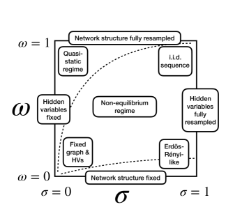
Figure 1: Two-parameter space of possible dynamics. The two parameters $(\sigma,\omega)\in[0,1]^{2}$ tune the rate of change of hidden variables and rate of resampling of links, respectively. In general, with dynamic hidden variables, link-structure is out-of-equilibrium relative to the configuration of hidden variables at any particular timestep, violating the Equilibrium Property. In the quasi-static regime (upper left) and along the upper and leftward boundary regions ($\omega=1$ and $\sigma=0$, respectively) the Equilibrium Property is recovered. In the lower-right regime, HVs are so randomized that network snapshots resemble Erdős-Rényi graphs. At $\sigma=1$ (right-hand boundary), all hidden variables are resampled at every timestep, but only a fraction $\omega$ of links resampled. If $\omega=0$ (lower boundary), the network structure remains fixed for all time, regardless of the hidden-variable dynamics. The dashed curves roughly designate the quasi-static regime and the Erdős-Rényi-like regime.

Name	Parameter Regime	Equilibrium Property	Tunable Persistence
Single Static Graph	$\omega=\sigma=0$	Yes	No
i.i.d. Graph Sequence	$\omega=\sigma=1$	Yes	No
Quasi-Static	$\alpha_{2}(\sigma,\omega)\approx 1$ (Equation 12)	Yes*	Yes
Complete link-resampling	$\omega=1,\sigma\in(0,1)$	Yes	Depends on $f$**
Deterministic HV-to-graph	$\omega=1,f:\mathcal{X}^{2}\rightarrow\{0,1\}$	Yes	Depends on $f$**
Complete HV-resampling	$\sigma=1,\omega\in(0,1)$	No	Yes ***
Fixed Hidden Variables	$\sigma=0$	Yes	Yes
Erdős-Rényi-like	$\sigma/\omega\gg 1$	No	No
Fixed graph structure	$\omega=0$	Yes****	No****

Table 1: Table of limiting cases of dynamics-parameters $(\sigma,\omega)$ for THVMs. The first and second columns provide a short-hand name and the associated parameter regime. The third column states whether the Equilibrium Property is satisfied, whereas the fourth column states whether the Persistence Property is satisfied (in a way that is tunable at any desired level, which for instance leaves out the case $\sigma=\omega=0$).

*In the quasi-static regime, $G^{(t)}$ will have arisen from an HV-configuration closely resembling $H^{(t)}$, due to a timescale-separation. This implies approximate, rather than exact, satisfaction of the Equilibrium Property.
       ** When $\omega=1$ although the persistence property is in general lost due to each possible edge being resampled at every timestep, there is still some persistence present, tuned by $\sigma$ and dependent upon the affinity function $f$.
       *** When $\sigma=1$ the persistence property is tunably satisfied at the level of graph-structure, but not at all at the level of hidden variables, which are completely resampled every timestep.
       **** In the case of $\omega=0$, the initial graph remains fixed for all time, while HVs change. Since the initial condition is sampled from the static model, this regime technically satisfies the Equilibrium Property. It does so both at the level of graphs and at the level of hidden variables, but not at all at the joint level. Persistence is not tunable at the level of graphs, but is at the level of hidden variables.

In this section we consider several limiting cases in the space of dynamics-parameters $(\sigma,\omega)\in[0,1]^{2}$, and some special-case categories of affinity function $f$. The resulting regimes exhibit a variety of qualitatively distinct behaviors. If $\sigma=\omega=0$, a single graph is sampled from the static model, and all of its hidden variables and links are held fixed for all $t$. To the opposite extreme, if $\sigma=\omega=1$, at each timestep, every node’s hidden variable is fully randomized, and then all possible links are re-evaluated, resulting in a sequence of independent and identically distributed (i.i.d.) instances of the static model. In either case, the Equilibrium Property is satisfied – but the Persistence Property is not for $\sigma=\omega=1$ (there is no persistence), whereas for $\sigma=\omega=0$ there is complete persistence.

In Sections IV.1, IV.2, IV.4, and IV.3, several other parameter regimes are analyzed. We discuss the behavior of temporal networks in each case, how well they qualify in terms of the Equilibrium and Persistence Properties, and their relations to preexisting commonly studied static network ensembles. Table 1 shows the different special cases, while a schematic picture of the space of dynamics-parameters is shown in Figure 1.

IV.1 Quasi-Static Regime ($\alpha_{2}(\sigma,\omega)\approx 1$)

Here we consider the parameter regime quantified by the condition $\alpha_{2}(\sigma,\omega)\approx 1$ (upper-left region of Figure 1), where

$$\alpha_{2}(\sigma,\omega)=\frac{\omega}{1-(1-\omega)(1-\sigma)^{2}}\in[0,1],$$ (12)

in which networks have both random link-structure and random hidden variables, and exhibit both the Persistence Property and the Equilibrium Property. The quantity $\alpha_{2}(\sigma,\omega)$ is a naturally-arising function characterizing how effective connection probabilities differ from their static-model counterparts (see Appendix A). The Equilibrium Property is satisfied due to sufficient timescale separation: link-resampling happens quickly enough relative to hidden-variable motion for $G^{(t)}$ to remain caught up with $H^{(t)}$. The dynamics can thus be considered quasi-static, in the sense of quasi-static transformations in classical equilibrium thermodynamics Landsberg (1956). Over time, the HV-configuration and link-structure both fully explore their respective spaces, functioning as a temporal network whose stationary distribution is the static hidden-variables model defined in Section III.1. Note that the Equilibrium Property is only approximately satisfied if $\alpha_{2}(\sigma,\omega)<1$, that approximation becoming exact only in limit of extreme timescale-separation or $\alpha_{2}(\sigma,\omega)=1$. Two regimes at the boundary of the quasi-static regime have exact satisfaction of the Equilibrium Property: $\omega=1$ (Section IV.2) and $\sigma=0$ (Section IV.3). Adding a third mechanism of dynamics allows for exact satisfaction of the Equilibrium Property at all $(\sigma,\omega)\in[0,1]^{2}$ (see Section VI).

IV.2 Complete link-resampling ($\omega=1$)

Here we consider the case $\omega=1$ (top region of Figure 1). This case resembles that of the quasi-static regime, but all links form based on current hidden-variable configurations, so there is no graph-encoded memory: $\mathcal{P}_{G}\left(G^{(t+1)}\left|G^{(t)},\mathbf{H}\right)\right.=\mathbb{P}\left(G^{(t+1)}\left|H^{(t+1)}\right)\right.$. The resulting Markov chain on $\mathcal{H}\times\mathcal{G}$ thus satisfies the Equilibrium Property exactly, as opposed to approximately in the quasi-static regime (Subsection IV.1). Link-structure when $\omega=1$ is more correlated over time than two i.i.d. samples from the SHVM (due to persistence in HV-configurations), but the specific level of persistence depends on the form of the affinity function $f(h,h^{\prime})$ and on $\sigma$. A variety of temporal network models have fully-resampled edges at each timestep Perra et al. (2012b); Papadopoulos and Flores (2019); Ghasemian et al. (2016).

As subset of the $\omega=1$ regime, consider THVMs with binary affinity function $f:\mathcal{X}^{2}\rightarrow\{0,1\}$. In this case all randomness comes from hidden variables, because $f$ deterministically maps HV-configurations to graphs. The static model’s conditional probability distribution in such cases is given by a product of indicator functions:

$$\mathbb{P}(G|H)=\prod_{1\leq i<j\leq n}\mathbf{1}\left\{A_{ij}=f\left(h_{i},h_{j}\right)\right\},$$ (13)

equal to $1$ if and only if $f(h_{i},h_{j})=A_{ij}$ for all $ij$, and equal to zero otherwise. Since the HV-dynamics $\mathcal{P}_{H}$ conserves $\rho$, and since $\omega=1$ ensures that all node-pairs have up-to-date links with respect to hidden variables, this model satisfies the Equilibrium Property exactly. The rate of HV-dynamics, and thus of link-dynamics, is controlled by $\sigma$ (but also influenced by the form of $f$). This regime encompasses sharp random geometric graphs (RGGs) of any kind Penrose et al. (2003); see Section V.2 for temporal RGGs with $\omega\in[0,1]$.

IV.3 Fixed Hidden Variables ($\sigma=0$)

Here we consider $\sigma=0$ (left region of Figure 1), in which case all HVs are frozen in place, ensuring satisfaction of the Equilibrium Property. The initial HV-configuration $H^{(1)}$ has the SHVM density $\rho$, but conditioning on some particular initial configuration $H^{(1)}$ yields fixed pairwise connection probabilities $p_{ij}=f\left(h_{i},h_{j}\right)$, resulting in temporal versions of edge-independent static networks Bollobás et al. (2007); Oliveira (2009); Lu and Peng (2012). Analytical expressions for link-dynamics can be written straightforwardly in terms of the set of values $\{p_{ij}\}_{1\leq i<j\leq n}$ and the parameter $\omega$. The transition probability $\mathcal{P}_{G}\left(G^{(t+1)}\left|G^{(t)}\right)\right.$ is

$$\mathcal{P}_{G}(G^{(t+1)}|G^{(t)})=\prod_{1\leq i<j\leq n}p^{A_{ij}^{(t)}\rightarrow A_{ij}^{(t+1)}}_{ij},$$ (14)

where $p_{ij}^{0\rightarrow 0}$, $p_{ij}^{0\rightarrow 1}$, $p_{ij}^{1\rightarrow 0}$, and $p_{ij}^{1\rightarrow 1}$ are respectively the non-link persistence, link-formation, link-removal, and link-persistence probabilities for node-pair $ij$. That is, $p^{\alpha\rightarrow\beta}_{ij}=\mathbb{P}(A_{ij}^{(t+1)}=\beta|A_{ij}^{(t)}=\alpha)$, given by:

$$p_{ij}^{\alpha\rightarrow\beta}= (1-\omega p_{ij})^{(1-\alpha)(1-\beta)}(\omega p_{ij})^{(1-\alpha)\beta}$$ (15)

$$\times(\omega(1-p_{ij}))^{\alpha(1-\beta)}(1-\omega(1-p_{ij}))^{\alpha\beta}.$$

Many static network models have independent edges with pre-defined connection probabilities, and thus can be made temporal as THVMs with $\sigma=0$. Examples include the Erdős-Rényi (ER) model Erdos and Renyi (1959) the (soft) stochastic block model (SBM) Anderson et al. (1992), and inhomogeneous random graphs Bollobás et al. (2007) with fixed coordinates.

The Persistence Property can be quantified by any of the numerous measures of graph dissimilarity Hartle et al. (2020), by application to graph-pairs at neighboring timesteps. A simple example in the $\sigma=0$ setting is the expected Hamming dissimilarity Hamming (1950),

$$\sum_{1\leq i<j\leq n} \mathbb{P}\left(A_{ij}^{(t)}\neq A_{ij}^{(t+1)}\right)$$ (16)

$$=\sum_{1\leq i<j\leq n}\left(p_{ij}^{1\rightarrow 0}p_{ij}+p_{ij}^{0\rightarrow 1}(1-p_{ij})\right)$$

$$=2\omega\sum_{1\leq i<j\leq n}p_{ij}(1-p_{ij}),$$

which simplifies substantially in some cases, for instance the ER model ($p_{ij}=p$ for all $ij$), leaving $2\omega p(1-p)\binom{n}{2}$.

Edge-resampling dynamics with fixed $p_{ij}$-values closely resembles dynamic percolation Steif (2009), which has been investigated in lattices Peres and Steif (1998), trees Khoshnevisan (2008) and ER graphs Roberts et al. (2018); Rossignol (2020), and also relates to edge-Markovian networks Clementi et al. (2010); Whitbeck et al. (2011); de Pebeyre et al. (2013).

IV.4 Complete resampling of hidden variables ($\sigma=1$)

Here we consider the case for which all hidden variables are resampled at every timestep ($\sigma=1$), so that no HV-driven structural persistence exists (right region of Figure 1). Note that walk-dynamics is parameterized by $\sigma$ so that $\sigma=1$ implies complete HV-randomization. If $\sigma=1$, correlations among links (and non-links) do still exist due to simultaneous resampling; the set of node-pairs selected for link-resampling at timestep $t$ form links based upon the same underlying hidden-variable configuration $H^{(t)}$. In this setting, $\omega$ quantifies the level of agreement among node-pairs as to what the HV-configuration is. For instance in spatial network models, if $\sigma=1$, then $\omega$ directly controls the level of geometry-induced correlations.

Given the HV-configuration at time $t$ and averaging over all past timesteps, node-pair $ij$ is connected with probability

$$\mathbb{P}\left(A_{ij}^{(t)}=1\left|h_{i}^{(t)},h_{j}^{(t)}\right.\right)=\omega f\left(h_{i}^{(t)},h_{j}^{(t)}\right)+(1-\omega)\langle f\rangle,$$ (17)

where $\langle f\rangle$ is the expected affinity of a pair of nodes with randomized HVs,

$$\langle f\rangle=\int_{\mathcal{X}^{2}}\nu(h)\nu(h^{\prime})f(h,h^{\prime})dhdh^{\prime}.$$ (18)

The expression 17 is an example of an effective connection probability which deviates from the static-model affinity function. A more general formula for the effective connection probability in the case of jump-dynamics and arbitrary $f(h,h^{\prime})$, $\sigma$, and $\omega$ is derived in Appendix A, and some special cases are described in the examples in Sections V.1,V.2,V.3,V.4. As $\omega\rightarrow 0$ with $\sigma=1$ (and in general for $\sigma/\omega\gg 1$), the model approaches a temporal version of the ER model, since each node-pair at the time of link-resampling will have completely randomized hidden variables; each edge will then independently exist with probability $\langle f\rangle$ if $0<\omega\ll 1$. If $\omega=0$ we have fixed graph structure, i.e. a network that simply remains as whatever the initially sampled graph was, but with dynamic hidden variables (for any $\sigma>0$).

V Temporal extensions of popular static network models

This section contains several examples of THVMs. In each subsection, we describe a static hidden-variables model, its temporal extension according to the modeling framework of Section III.2, the effective connection probability that arises due to the dynamics, and offer some additional discussion. We specifically consider temporal extensions of the following static network models: stochastic block models Karrer and Newman (2011), random geometric graphs Penrose et al. (2003), hypersoft configuration models van der Hoorn et al. (2018), and hyperbolic graphs Krioukov et al. (2010).

V.1 Temporal Stochastic Block Models

This subsection considers temporal extensions of stochastic block models (SBMs), which are used to model community structure in networks Anderson et al. (1992); Karrer and Newman (2011); Peixoto (2012, 2017).

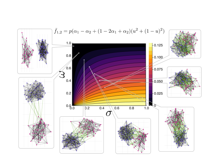
Figure 2: Snapshots of a temporal stochastic block model: a modular network with dynamic group-assignments and link-resampling. The $n=100$ nodes are partitioned into two groups with group-membership probabilities $\varrho_{1}=0.4=1-\varrho_{2}$, and group-memberships change in time by group-resampling with probability $\sigma$. The affinity function is $f_{q,q^{\prime}}=p\mathbf{1}\{q=q^{\prime}\}$ with $p=0.25$, disallowing inter-group connections in the static model. Network snapshots are displayed via a spring-force layout algorithm Kobourov (2012), for various parameters $(\sigma,\omega)$ such that networks span a variety of structural outcomes. Node-coloration is by group-membership, and link-coloration is black for within-group links and green for between-group links. In the central panel, the effective connection probability $\bar{f}_{1,2}$ between communities is plotted. Outside of the quasi-static regime, group-membership dynamics is fast enough for a substantial number of inter-group links to exist ($\bar{f}_{1,2}>0$), despite the inter-group connection formation probability being $f_{1,2}=0$.

V.1.1 Static Hyperparametric SBMs

We consider a static network with conditionally Bernoulli-distributed edges amongst $n$ nodes $j\in[n]$, each node having been randomly assigned to one of $m$ groups (a.k.a. communities, blocks, colors). Each node $j$ independently draws a group-index $q_{j}\in[m]=\{1,...,m\}$ from probability distribution $\varrho=\{\varrho_{q}\}_{q\in[m]}$. Each node-pair then connects with probability $f_{q_{i},q_{j}}$. In this definition, the group-memberships $\{q_{j}\}_{j\in[n]}$ are not externally specified as model parameters – rather, their distribution $\varrho$ is specified. Thus, the group-memberships are hyperparameters, and we refer to these static networks as hyperparameteric SBMs or hyper-SBMs (equivalent to inhomogeneous random graphs with hidden color Söderberg (2003, 2002)). The expected number of nodes $n_{q}$ in a given block $q$ is $\langle n_{q}\rangle=n\varrho_{q}$, and the joint distribution of $\{n_{q}\}_{q\in[m]}$ is multinomial. Note that this model could be formulated with continuous HVs as per Section III.1, but we instead use discrete HVs for simplicity (see Appendix H for the continuous-to-discrete mapping). As an illustrative example to be used throughout this section, we consider the case of $m=2$ groups, with $\varrho_{1}=1-\varrho_{2}=u$. The within-group affinity is $p=f_{1,1}=f_{2,2}$, and the between-group affinity is zero ($f_{1,2}=0$).

V.1.2 Temporal hyper-SBMs

To make the hyper-SBM dynamic, at each timestep $t\in\{2,...,T\}$ each node $i$ with probability $\sigma$ resamples its group-index $q_{i}^{(t)}$ from distribution $\varrho$, and then each node-pair $ij$ with probability $\omega$ resamples $A_{ij}^{(t)}$ with connection probability $f_{q_{i}^{(t)},q_{j}^{(t)}}$. Thus,

$$\mathbb{P}\left(q_{i}^{(t)}=q^{\prime}\left|q_{i}^{(t-1)}=q\right.\right)=(1-\sigma)\mathbf{1}\{q=q^{\prime}\}+\sigma\varrho_{q^{\prime}},$$ (19)

and

$$\mathbb{P}\left(A_{ij}^{(t)}=1\left|A_{ij}^{(t-1)},q_{i}^{(t)},q_{j}^{(t)}\right.\right)=(1-\omega)A_{ij}^{(t-1)}+\omega f_{q_{i}^{(t)},q_{j}^{(t)}}.$$ (20)

See Figure 2 for visualized embeddings of network snapshots from the stationary distribution of the example $m=2$, $\varrho_{1}=u=1-\varrho_{2}$, $f_{q,q^{\prime}}=p\mathbf{1}\{q=q^{\prime}\}$.

V.1.3 Effective connection probabilities in hyper-SBMs

The block-dynamics of nodes in temporal hyper-SBMs introduces several novel features to the system. First, pairwise affinities change over time. Second, the set of all existing links at time $t$ need not have arisen from the group-assignments of time $t$. Temporal snapshots in general thus deviate from the static model – the Equilibrium Property does not necessarily hold. However, even if snapshots do not resemble the static model, they do resemble a static model – an effective SBM. Consider two nodes, with current group-indices $q,q^{\prime}$. Averaging over all past values of hidden variables, we obtain the effective connection probability $\bar{f}_{q,q^{\prime}}$ for dynamic hyper-SBMs. Since the SBM case is directly obtainable from discretization of the continuous model (see Appendix H) we can use a discrete version of the general formula derived in Appendix A, namely:

$$\bar{f}_{q,q^{\prime}} =\alpha_{2}f_{q,q^{\prime}}$$ (21)

$$\ \ +(\alpha_{1}-\alpha_{2})\left(\langle f_{q,\cdot}\rangle+\langle f_{q^{\prime},\cdot}\rangle\right)$$

$$\ \ +(1-2\alpha_{1}+\alpha_{2})\langle f\rangle,$$

where coefficients $\alpha_{b}(\sigma,\omega)$ for $b\in\{1,2\}$ are given by

$$\alpha_{b}=\frac{\omega}{1-(1-\omega)(1-\sigma)^{b}},$$ (22)

and marginally-averaged affinities are

$$\langle f_{q,\cdot}\rangle =\sum_{q^{\prime}}\varrho_{q^{\prime}}f_{q,q^{\prime}},$$ (23)

$$\langle f\rangle =\sum_{q}\varrho_{q}\langle f_{q,\cdot}\rangle=\sum_{q,q^{\prime}}\varrho_{q}\varrho_{q^{\prime}}f_{q,q^{\prime}}.$$

Note that when $\sigma=1$ we have $\alpha_{1}(1,\omega)=\alpha_{2}(1,\omega)=\omega$ and Equation 21 reduces to the form of Equation 17. In the simple example case ($m=2,\varrho_{1}=u,f_{q,q^{\prime}}=p\mathbf{1}\{q=q^{\prime}\}$), terms in $\bar{f}_{q,q^{\prime}}$ are evaluated as:

$$\langle f_{1,\cdot}\rangle =up,$$ (24)

$$\langle f_{2,\cdot}\rangle =(1-u)p,$$

$$\langle f\rangle =p(u^{2}+(1-u)^{2}),$$

from which the formula for $\bar{f}_{q,q^{\prime}}$ becomes

$$\bar{f}_{q,q^{\prime}} =\alpha_{2}p\mathbf{1}\{q=q^{\prime}\}$$ (25)

$$\ \ +(\alpha_{1}-\alpha_{2})\left\{\begin{array}[]{cc}2up,&q=q^{\prime}=1\\ 2(1-u)p,&q=q^{\prime}=2\\ p&q\neq q^{\prime}\end{array}\right.$$

$$\ \ +(1-2\alpha_{1}+\alpha_{2})p(u^{2}+(1-u)^{2}).$$

In particular, the between-group effective connection probability becomes

$$\bar{f}_{1,2}=p\left(\alpha_{1}-\alpha_{2}+(1-2\alpha_{1}+\alpha_{2})(u^{2}+(1-u)^{2})\right),$$ (26)

which is visualized in Figure 2. In the extreme case of $\sigma/\omega\gg 1$ all links form between nodes with effectively random group-assignments, making all pairs equally likely to connect, and reducing the system to a temporal Erdős-Rényi network of connection probability $p(u^{2}+(1-u)^{2})$.

V.1.4 Temporal hyper-SBMs discussion

Interesting examples of Qualitative Realism arise in temporal hyper-SBMs. For instance, group-dynamics of nodes yields inter-group connectivity, as is observed in real systems. If someone joins a different club, switches political party, or emigrates to a new country, they at first primarily carry ties to their original group – and thus upon changing group-membership, they suddenly have many inter-group links – not because of inter-group link-formation, but because of dynamic group-membership. Likewise, within-group connectivity can be lower than in the static model, as is the case in real systems due to nodes having recently arrived from another group, or from neighbor-nodes having recently departed. These effects arise outside the quasi-static regime, so we speculate that in some cases the non-equilibrium regime can better emulate real-world systems. We also note that we here considered group-resampling HV-dynamics (a discrete version of jump-dynamics), but we could also consider a general Markov chain on group-assignments with stationary distribution $\varrho$.

V.2 Temporal Random Geometric Graphs

In this section we describe THVMs arising from static random geometric graphs (RGGs), which model the influence of an underlying geometry on graph-structure Penrose et al. (2003).

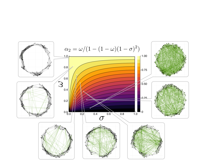
Figure 3: Snapshots of a temporal random geometric graphs: a geometrically-embedded network with dynamic node-coordinates and link-resampling. Coordinates of $n=100$ nodes are sprinkled uniformly into a 1D ring of unit circumference, and change in time via jump-dynamics (coordinate-resampling with probability $\sigma$). The affinity as a function of distance is $f(x)=\mathbf{1}\{x\leq r\}$, where $r=0.1$ is the connection radius, disallowing long-ranged links in the static model. Snapshots are shown at various values of $(\sigma,\omega)$, with angular positions equal to $2\pi$ times spatial coordinates, and radial positions set to $1$ with some added random noise. Link coloration is according to length: black links are of distances $x\leq r$ whereas green links are of distances $x>r$. In the central panel, the function $\alpha_{2}(\sigma,\omega)\in[0,1]$ is visualized, which encodes the level of locality in temporal RGGs (see Equation 27).

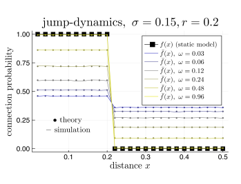
Figure 4: The effective connection probability, in theory and simulation, for 1D RGGs at various values of the dynamics-parameters $(\sigma,\omega)$. The static model affinity-function $f(x)$ is plotted with square markers. The solid lines are numerical estimates of the effective connection probability $\bar{f}(x)$ (with $\omega$ increasing as colors change from blue to yellow), whereas the dotted lines are the theoretical effective connection probability (Equation 27).

V.2.1 Static Random Geometric Graphs

In random geometric graphs (RGGs), nodes are assigned spatial coordinates as hidden variables, and node-pairs are linked if their coordinates are closer than some threshold distance $r$. Hence the affinity is binary, $f(h_{i},h_{j})=\mathbf{1}\{\mathrm{d}_{\mathcal{X}}(h_{i},h_{j})\leq r\}$, with $\mathrm{d}_{\mathcal{X}}:\mathcal{X}^{2}\rightarrow[0,\infty)$ denoting the geodesic distance in latent space $\mathcal{X}$. Examples of well-studied RGGs include Euclidean RGGs with periodic or nonperiodic boundary conditions Penrose et al. (2003), spherical RGGs Allen-Perkins (2018), and hyperbolic RGGs (the hyperbolic model with inverse-temperature parameter $\beta=\infty$ Krioukov et al. (2010)). As a primary example we consider a simple one-dimensional RGG with periodic boundary conditions: $\mathcal{X}=[0,1)$ and $\mathrm{d}_{\mathcal{X}}(h_{i},h_{j})=1/2-|1/2-|h_{i}-h_{j}||$.

V.2.2 Temporal RGGs

To go from static RGGs to temporal RGGs, we incorporate coordinate-dynamics and link-resampling dynamics. We consider here jump-dynamics, each node resampling its coordinate according to the static-model density $\nu$, with probability $\sigma$, each timestep $t\in\{2,...,T\}$ (the coordinate density follows Equation 6, with $\nu(h)=1$ for the uniform density on the unit interval). Link-resampling happens independently for each node-pair with probability $\omega$ each timestep. Since RGGs have deterministic connectivity, link-resampling of $ij$ at time $t$ guarantees that $A_{ij}^{(t)}=1$ if $\mathrm{d}_{\mathcal{X}}(h_{i}^{(t)},h_{j}^{(t)})\leq r$ and $A_{ij}^{(t)}=0$ otherwise. But if $ij$’s connectivity is not resampled at time $t$, links may fall out-of-equilibrium with respect to coordinates. Note that we could also study temporal RGGs with walk-dynamics, with either periodic or reflecting boundary conditions; for simplicity, we study jump-dynamics here, leaving temporal RGGs with walk-dynamics for a future study.

V.2.3 Effective connection probabilities in temporal RGGs

We now describe the effective connection probability $\bar{f}(x)$ for RGGs between pairs of nodes for arbitrary $(\sigma,\omega)$. The expression for $\bar{f}(x)$ in temporal RGGs is derived in Appendix B, and the result is provided here:

$$\bar{f}(x)=\alpha_{2}\mathbf{1}\{x\leq r\}+2r(1-\alpha_{2}).$$ (27)

The quantity $\alpha_{2}=\alpha_{2}(\sigma,\omega)$, defined in Equation 22, directly governs the level of locality in temporal RGGs. See Figure 3 for a visualization of the function $\alpha_{2}(\sigma,\omega)$ and of network snapshots across a range of $(\sigma,\omega)$-values. The effective connection probability $\bar{f}(x)$ has a step-like form, with connection probability $\alpha_{2}+2r(1-\alpha_{2})$ for all $x\leq r$ and $2r(1-\alpha_{2})$ for all $x>r$. The above effective connection probability agrees perfectly with the results of numerical simulations, see Figure 4.

V.2.4 Temporal RGGs discussion

The naturally arising function $\alpha_{2}(\sigma,\omega)\in[0,1]$ describes the level of locality in network snapshots (see Figure 3), and quantifies the Equilibrium Property. It interpolates between the case of RGGs ($\alpha_{2}(\sigma,\omega)=1$) and ER graphs ($\alpha_{2}(\sigma,\omega)=0$), resembling the structural transition of the Watts-Strogatz model Watts and Strogatz (1998). In this case, all links form locally, and it is dynamics of node positions that induces the transition (alongside formation of local links at nodes’ new locations); a similar phenomenon has been observed in contagion-dynamics among mobile agents Buscarino et al. (2008). Also note, in dynamic RGGs, links can exist that were not possible in the static model model: links of length greater than $r$, since the effective connection probability $\bar{f}(x)$ no longer goes completely to zero for $x>r$ (see Equation 27). This is related to phenomena observed in real-world networks: pairs of people may form friendships locally, but maintain those friendships after becoming geographically separated, resulting in the existence of long-ranged social ties that would not likely have formed at that distance. Likewise, the function $\bar{f}(x)$ is also less than one for distances $x\leq r$, allowing for non-links that would be impossible in the static model. That phenomenon also appears in real-world systems: instead of individuals knowing everyone in their local vicinity, non-links between closeby pairs may exist, due to them having only recently become proximate. As with the case of temporal hyper-SBMs, these examples of Qualitative Realism are in conflict with the Equilibrium Property. Note also that similar deviations of $\bar{f}(x)$ relative to $f(x)$ occur in THVMs arising from soft random geometric graphs Penrose et al. (2016); Wilsher et al. (2020); Kaiser and Hilgetag (2004); Dettmann and Georgiou (2016), for example the $\mathbb{H}^{2}$ model (see Section V.4).

V.3 Temporal Hypersoft Configuration Model

In this section we consider a dynamic version of hypersoft configuration models (HSCMs), which model networks with degree-heterogeneity van der Hoorn et al. (2018).

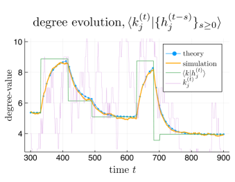
Figure 5: Expected degree over time of a node in a temporal hypersoft configuration model with jump-dynamics of hidden variables. Each node’s expected degree (blue dotted curve) equilibrates towards its current static-model expected degree (green solid curve), as per Equation LABEL:eq:degree_dynamics. In any realization, the actual degree over time fluctuates (purple curve), but its ensemble-average (orange solid curve) behaves as predicted. The average was obtained by simulating $1000$ realizations with $(n,\langle k\rangle,\gamma,\omega,\sigma)=(200,8,2.8,0.04,0.01)$, keeping the HV-trajectory $\{h_{j}^{(t)}\}_{t=1}^{T}$ of a single node $j$ fixed across trials.

V.3.1 Static Hypersoft Configuration Model

The static model we now consider is the hypersoft configuration model van der Hoorn et al. (2018); Voitalov et al. (2020) (HSCM), a hyperparametric version of a soft configuration model (SCM). SCMs come in several varieties such as the Chung-Lu model Chung and Lu (2002), inhomogeneous random graphs Bollobás et al. (2007), and the Norros-Reittu model Norros and Reittu (2006). Node-pairs connect with $A_{ij}$-values being independent (typically Bernoulli or Poisson distributed), such that on average, each node has a particular degree-value. In hyperparametric SCMs, that degree-value is randomly assigned, according to some specified distribution of expected degrees. For example, one way to obtain SCMs with a degree distribution that is Pareto-mixed Poisson (with, say, power-law tail-exponent $\gamma$ and expected degree $\langle k\rangle$), is for nodes $j\in[n]$ to be assigned hidden variables $h_{j}\in[h_{-},\infty)$ drawn from a Pareto density $\nu(h)=(\gamma-1)h_{-}^{\gamma-1}h^{-\gamma}$, with minimal HV-value $h_{-}=(\gamma-2)\langle k\rangle/(\gamma-1)$, and then for node-pairs to be connected with probability

$$f(h_{i},h_{j})=\frac{1}{1+n\langle k\rangle/h_{i}h_{j}}\approx\frac{h_{i}h_{j}}{n\langle k\rangle},$$ (28)

the approximation holding when $h_{i}h_{j}/n\langle k\rangle\ll 1$. The expected degree of a node $i$ in the static model is

$$\langle k_{i}|h_{i}\rangle=(n-1)\int_{h_{-}}^{\infty}f(h_{i},h)\nu(h)dh\approx h_{i}.$$ (29)

The actual degrees of nodes are sharply peaked around their expected degrees, and thus the above implies that the degree distribution itself likewise has a power-law tail with exponent $\gamma$ and mean $\langle k\rangle$.

V.3.2 Temporal HSCMs

Now we consider a temporal version of HSCMs. At each timestep, each node $j$, with probability $\sigma$, resamples its hidden variable $h_{j}^{(t)}$ from the static-model HV-density $\nu$ (jump-dynamics). Then, each node-pair $ij$ ($1\leq i<j\leq n$), with probability $\omega$, has its indicator-variable $A_{ij}^{(t)}$ resampled from a Bernoulli of mean $f(h_{i}^{(t)},h_{j}^{(t)})$.

In the static model, the HV-value $h_{j}$ alone determines the expected degree $\langle k_{j}|h_{j}\rangle$. But in the temporal version, the quantity $h_{i}^{(t)}$ is time-evolving, and the expected degree dynamically trails behind the static-model expected degree, equilibrating at a geometric pace (See Figure 5):

$$\mathbb{E}\left[k_{i}^{(t)}\left|\left\{h_{i}^{(t-s)}\right\}_{s\geq 0}\right.\right]$$ (30)

$$=(n-1)\omega\sum_{s\geq 0}(1-\omega)^{s}\int_{h_{-}}^{\infty}f\left(h_{i}^{(t-s)},h\right)\nu(h)dh$$

$$=\omega\sum_{s\geq 0}(1-\omega)^{s}\left\langle k_{i}\left|h_{i}^{(t-s)}\right.\right\rangle.$$

We can also average the above over all hidden-variable values at timesteps earlier than $t$, to obtain an effective expected degree that depends only on $h_{j}^{(t)}$. To do this, we use the probability density of $h_{j}^{(t-s)}$ given $h_{j}^{(t)}$ under jump-dynamics:

$$P_{s}\left(x\left|h_{j}^{(t)}\right.\right)=(1-\sigma)^{s}\mathbf{1}_{h_{j}^{(t)}}(x)+\left(1-(1-\sigma)^{s}\right)\nu(x),$$ (31)

Averaging Equation LABEL:eq:degree_dynamics over HVs at all timesteps $t-s$ for $s>0$,

$$\mathbb{E}\left[k_{i}^{(t)}\left|h_{i}^{(t)}\right.\right] =\omega\sum_{s\geq 0}(1-\omega)^{s}\int_{h_{-}}^{\infty}P_{s}\left(x\left|h_{i}^{(t)}\right.\right)\langle k_{i}|x\rangle dx$$ (32)

$$=\alpha_{1}\left\langle k_{i}\left|h_{i}^{(t)}\right.\right\rangle+(1-\alpha_{1})\langle k\rangle,$$

where $\alpha_{1}(\sigma,\omega)=\omega\left/\left(1-(1-\omega)(1-\sigma)\right)\right.$. In this case $\alpha_{1}$ measures the level of equilibration of node-neighborhoods to their expected sizes. Having $\alpha_{1}\approx 1$ indicates the quasi-static regime whereas $\alpha_{1}\approx 0$ indicates an averaged-out behavior so that the expected degree of any given node is simply the expected average degree $\langle k\rangle$ of the network.

V.3.3 Effective connection probabilities in temporal HSCMs

We now discuss effective connection probabilities in HSCMs. The formula derived in Appendix A applies, but note that the affinity $f(h,h^{\prime})$ (Equation 28) is a function only of the product $\psi=hh^{\prime}$. Thus we can examine the effective connection probability as a function of $\psi$, denoted $\bar{f}(\psi)$. In order to calculate $\bar{f}(\psi)$ we first must compute the probability density of a product of hidden variables in past timesteps, given the value of the product at the current timestep. We then sum the expected affinity given the product, weighted by $p_{s}=\omega(1-\omega)^{s}$, over all past timesteps $s>0$. These calculations require a variety of intermediate steps, and are described in Appendix C.

V.3.4 Temporal HSCMs discussion

Note that in HSCMs, non-equilibrium dynamics reduces degree-heterogeneity; nodes with large HV-values only transiently retain them. Equilibration, on the other hand, allows for a full structural expression of the nodes’ internal heterogeneity. This implies that extremely heterogeneous real-world networks, if described by these models, would typically be in the quasi-static regime. We only considered jump-dynamics here (resampling of static-model expected degree-values), but we could alternatively study walk-dynamics, where nodes’ HVs undergo Brownian-like motion in a way that preserves $\nu$. This could be achieved straightforwardly as described in D, alongside reflecting boundaries as studied in Appendix E.

V.4 Temporal Hyperbolic Graphs

In this section we consider a temporal extension of the hyperbolic model Krioukov et al. (2010) (the $\mathbb{H}^{2}$ model, for short), a geometry-based network model simultaneously exhibiting sparsity, clustering, small-worldness Bringmann et al. (2016); Friedrich and Krohmer (2018), degree heterogeneity, community structure Faqeeh et al. (2018), and renormalizability García-Pérez et al. (2018).

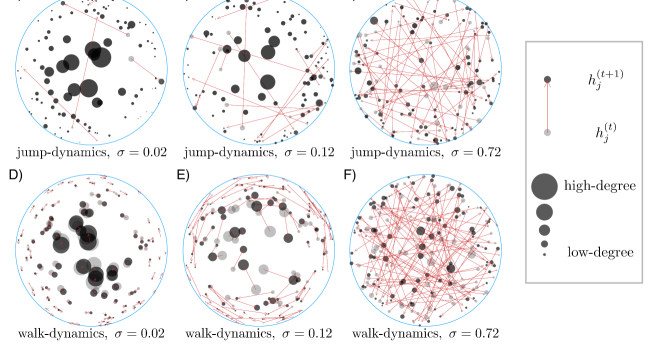
Figure 6: Hidden-variable dynamics of nodes in a temporal $\mathbb{H}^{2}$ model, at increasing values of $\sigma$, with fixed $\omega=0.1$. In each subplot, node-coordinates for $100$ random nodes are shown at two adjacent timesteps, from a network with parameters $(n,\gamma,\beta,R)=(500,2.2,5,8)$. Each arrow points from the coordinate-location of a node at a given timestep (grey) to the coordinate-location of the same node at the next timestep (black). Subplots (A,B,C) depict jump-dynamics (coordinate-resampling with probability $\sigma$, otherwise remaining in place), whereas subplots (D,E,F) depict walk-dynamics (all nodes move to neighboring locations, with mean step-length parameterized by $\sigma$). Marker sizes are proportional to node degree-values. For small $\sigma/\omega$ (subplots A and D), nodes’ existing connections have arisen from approximately the present coordinates, making snapshots closely resemble the static hyperbolic model, as seen e.g. by the exhibited degree-heterogeneity. For larger $\sigma/\omega$ (subplots B and E), connections have arisen via mixtures of past and present coordinates, reducing degree-heterogeneity. For very large $\sigma/\omega$ (subplots C and F), the system behaves similarly to a temporal Erdős-Rényi network.

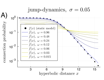
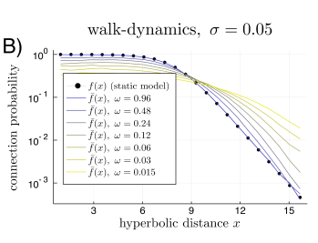
Figure 7: Effective connection probability function $\bar{f}(x)$ in snapshots of a temporal hyperbolic model with $(n,\gamma,\beta,R)=(500,2.2,5,8)$, for various values of $\omega$. With slower link-resampling (smaller $\omega$), links are increasingly allowed to dynamically stretch before being removed by link-resampling, resulting in deviations from the static-model affinity $f(x)$ (black dotted line). Coloration of the curve $\bar{f}(x)$ is from yellow to blue as $\omega$ increases. The upper panel, A), shows the case of jump-dynamics of coordinates. The lower panel, B), shows the case of walk-dynamics of coordinates. The choice of coordinate-dynamics is consequential in the non-equilibrium regime, despite each having the same stationary density.

V.4.1 Static $\mathbb{H}^{2}$ model

The $\mathbb{H}^{2}$ model is parameterized by a number of nodes $n$, average degree $\langle k\rangle$, power-law exponent $\gamma$, and inverse-temperature $\beta$ (which tunes the level of clustering). Hidden variables are polar coordinates, $h_{j}=(\theta_{j},r_{j})$, namely a radial coordinate $r_{j}\in[0,R]$ encoding the popularity of node $j$ and an angular coordinate $\theta_{j}\in[0,2\pi)$, encoding the similarity of node $j$ to other nodes. These coordinates are sampled according to separable density $\nu(\theta,r)=\nu_{ang}(\theta)\nu_{rad}(r)$ where angles are distributed uniformly ($\nu_{ang}(\theta)=1/2\pi)$ and radii have an exponentially growing density,

$$\nu_{rad}(r)=\frac{\gamma-1}{2}\frac{\sinh\left(\frac{\gamma-1}{2}r\right)}{\cosh\left(\frac{\gamma-1}{2}R\right)-1},$$ (33)

where $R=R(n,\langle k\rangle,\beta,\gamma)$ is selected so that the mean degree is $\langle k\rangle$. The static-model affinity of node-pair $ij$ is a Fermi-Dirac function Kardar (2007) (a sigmoid) of the hyperbolic geodesic distance $x_{ij}$ between $i$ and $j$,

$$f(h_{i},h_{j})=f(x_{ij})=1\left/\left(1+e^{(\beta/2)\left(x_{ij}-R\right)}\right)\right.,$$ (34)

where $x_{ij}=x_{ij}(h_{i},h_{j})$ is given by

$$\cosh(x_{ij})= \cosh(r_{i})\cosh(r_{j})$$ (35)

$$-\sinh(r_{i})\sinh(r_{j})\cos(\theta_{ij}),$$

with $\theta_{ij}=\pi-\left|\pi-|\theta_{i}-\theta_{j}|\right|$. The connection probability and coordinate-density in this model result in power-law degree distributions (but could also give rise to other degree distributions if the radial coordinate-density was different), a similar feature to that exhibited by HSCMs – but also, the geometry arising from inclusion of the angular coordinate yields a large clustering coefficient and spatially localized link-structure, making this model also similar to standard RGGs. Increasing the parameter $\beta$ yields more localized link-structure, approaching a step function as $\beta\rightarrow\infty$, leaving in that case an RGG (see Section V.2.1) on the hyperbolic disk. As $\beta\rightarrow 0$, typical link-lengths approach the system size and the model behaves similarly to the HSCM (see Section V.3.1).

V.4.2 Temporal $\mathbb{H}^{2}$ model

To temporally extend the $\mathbb{H}^{2}$ model, we allow coordinate dynamics so that each node $j$ exhibits a trajectory in the hyperbolic disk, $h_{j}^{(t)}=(\theta_{j}^{(t)},r_{j}^{(t)})$ for $t\in[T]$. For jump-dynamics, each node jumps to a random location according to density $\nu(\theta,r)$, with probability $\sigma$ each timestep. For walk-dynamics, each node $j$ steps to a random location $h_{j}^{(t+1)}$ having angular and radial coordinates adjusted to relatively closeby values, with increasingly large steps for larger $\sigma$-values; we describe the details of $\mathbb{H}^{2}$ walk-dynamics in Appendix F. Dynamics of nodes on the hyperbolic disk is visualized in Figure 6, for both jump-dynamics and walk-dynamics. For $\sigma\ll 1$, nodes rarely resample their coordinates (in jump-dynamics) and step to only very localized regions (in walk-dynamics). On the other hand for $\sigma\approx 1$, almost all nodes resample their coordinates at each timestep (in jump-dynamics) or move to a nearly-randomized location (in walk-dynamics). We note that many other natural and interesting choices for HV-dynamics exist, as we discuss in Section VIII and Appendix F.

V.4.3 Effective connection probabilities in the temporal $\mathbb{H}^{2}$ model

In the temporal $\mathbb{H}^{2}$ model considered here, the effective connection probability $\bar{f}(x)$ no longer remains in the standard Fermi-Dirac form of $f(x)$ (see Figure 7). With decreasing $\omega/\sigma$, the connection probability function smooths out and extends to a longer range due to links being stretched more rapidly (for walk-dynamics), or more frequently (for jump-dynamics). This effect is more uniform and extends all the way out to long ranges for jump-dynamics, whereas it is more localized for walk-dynamics, for any given non-equilibrium value of $(\sigma,\omega)$.

Since the coordinates of $\mathbb{H}^{2}$ reflect popularity and similarity attributes, the effective connection probability and other non-equilibrium effects arising when outside of the quasi-static regime have specific interpretations. The set of current links arose from nodes having been connected at past timesteps when their previous similarity attributes were compatible (small hyperbolic distance); in real networks, such links may persist into the future even if the similarity attributes change. For instance with social networks, consider friendships on Facebook, followers on Twitter, or author collaborations: similarity between connected pairs may decrease over time, but they tend to remain connected. Likewise, it could take some time for two people that become more similar to discover one another and to connect, in an online or traditional social network.

V.4.4 Temporal $\mathbb{H}^{2}$ model discussion

Outside of the quasi-static regime, snapshots $G^{(t)}$ do not fully resemble the static $\mathbb{H}^{2}$ model – the Equilibrium Property is in general violated (despite the fact that each link was formed via the static-model connection probability corresponding to the pairwise distance at the time of that link’s formation). This phenomenon results in reduced clustering because links become spread out across the space rather than being localized amongst neighboring groups of nodes. Degree-heterogeneity is also suppressed, as is the case for the temporal HSCM (see Section V.3), because nodes accumulating large numbers of links due to being near the disk’s center do not stay near the disk’s center indefinitely. Clustering and heterogeneity arise in the static $\mathbb{H}^{2}$ model due to the correlations in links from the underlying geometry. But in the static model, all links (and non-links) arise from the same underlying coordinate-configuration. When coordinates are dynamical, these correlations are weaker; nodes are linked with probabilities arising as a mixture of past and present coordinate-configurations.

VI Link-updating in response to hidden-variable dynamics

Finally, we describe an additional dynamical mechanism that can be incorporated to achieve the Equilibrium Property exactly in temporal hidden-variables models, while retaining the Persistence Property, for all values of $\sigma$ and $\omega$: links are updated directly in response to changes in hidden variables, rather than only through link-resampling, to keep connection probabilities up-to-date (we refer to this mechanism as link-response). In this model variant, $G^{(t+1)}$’s probability distribution depends on each of $G^{(t)}$, $H^{(t+1)}$, and $H^{(t)}$, rather than on just the former two. We illustrate the mechanism at first in the case of $\omega=0$. Suppose node-pair $ij$ has a link with probability $p_{ij}=f(h_{i},h_{j})$, and that HVs $(h_{i},h_{j})$ are updated to become $(h^{\prime}_{i},h^{\prime}_{j})$ in the next timestep. To ensure that the pair is then connected with probability $p_{ij}^{\prime}=f(h^{\prime}_{i},h^{\prime}_{j})$, we selectively delete now-less-likely edges between connected pairs and selectively add now-more-likely edges between unconnected pairs. In particular:

• If $p_{ij}^{\prime}\geq p_{ij}$, then $A_{ij}=1\Rightarrow A^{\prime}_{ij}=1$, and $A_{ij}=0\Rightarrow$ add link with probability $q^{+}_{ij}$,

• If $p_{ij}^{\prime}\leq p_{ij}$, then $A_{ij}=0\Rightarrow A^{\prime}_{ij}=0$, and $A_{ij}=1\Rightarrow$ remove link with probability $q^{-}_{ij}$.

The outcome needs to result in $\mathbb{P}(A^{\prime}_{ij}=1|h_{i}^{\prime},h_{j}^{\prime})=p^{\prime}_{ij}$. Thus,

• If $p_{ij}^{\prime}\geq p_{ij}$, the new connection probability satisfies $p^{\prime}_{ij}=p_{ij}+(1-p_{ij})q^{+}_{ij}$. Hence, $q^{+}_{ij}=1-\frac{1-p^{\prime}_{ij}}{1-p_{ij}}$.

• If $p_{ij}^{\prime}\leq p_{ij}$, the new connection probability satisfies $1-p^{\prime}_{ij}=p_{ij}q^{-}_{ij}+(1-p_{ij})$. Hence, $q^{-}_{ij}=1-\frac{p^{\prime}_{ij}}{p_{ij}}$.

Note that if $p^{\prime}_{ij}=p_{ij}$, then $q^{+}_{ij}=q^{-}_{ij}=0$; no links will form or break unless pairwise affinities change. Denoting $p_{ij}^{(t)}=f(h_{i}^{(t)},h_{j}^{(t)})$ for $t\in\{1,...,T\}$, the graph transition probability given $\mathbf{H}$ becomes:

$$\mathcal{P}_{G}\left(\left.G^{(t+1)}\right|G^{(t)},\mathbf{H}\right)=\prod_{1\leq i<j\leq n}Y_{ij}\left(A_{ij}^{(t+1)}\left|A_{ij}^{(t)},\mathbf{H}\right)\right.,$$ (36)

with $Y_{ij}:\{0,1\}\rightarrow[0,1]$ denoting the conditional adjacency-element probability distribution. For any $\omega\in[0,1]$, we have:

$$Y_{ij}\left(1\left|A_{ij}^{(t)},\mathbf{H}\right)\right.=\omega p_{ij}^{(t+1)}+(1-\omega)K_{ij}\left(A_{ij}^{(t)},\mathbf{H}\right),$$ (37)

where $K_{ij}(A_{ij}^{(t)},\mathbf{H})$ incorporates the link-response dynamics:

$$K_{ij}\left(A_{ij}^{(t)},\mathbf{H}\right)= \mathbf{1}\left\{p_{ij}^{(t+1)}\geq p_{ij}^{(t)}\right\}\left(q^{+}_{ij}\left(1-A_{ij}^{(t)}\right)+A_{ij}^{(t)}\right)$$ (38)

$$+\mathbf{1}\left\{p_{ij}^{(t+1)}\leq p_{ij}^{(t)}\right\}(1-q^{-}_{ij})A_{ij}^{(t)}.$$

With the inclusion of link-response, arbitrary static hidden-variable networks can be extended to temporal settings while satisfying the Equilibrium Property exactly (See Appendix VI for a full derivation), and the Persistence Property in a tunable fashion. Allowing $\omega>0$ does not alter the Equilibrium Property’s exact validity, and it provides a more tunable level of structural persistence.

With $G^{(t)}$ indistinguishable from a static-model realization, all non-equilibrium phenomena of the types discussed in V.1, V.2, V.3, and V.4 are prevented – this can either enhance or hinder Qualitative Realism, depending on the context. If a single node’s HV is changed, it will need to re-evaluate connections to all other nodes for which affinities have changed. This could be realistic in some cases, since nodes themselves may be at the most liberty to re-evaluate their connections. In other cases, more gradual structural transitions may be preferred. This model-variant could thus serve well as a temporal null model, especially for temporal networks with snapshots well-described by an SHVM. Despite structure of THVMs with link-response being identical to that of SHVMs, all dynamical features are open for study and for comparison to real-world networks.

VII Related Work

We briefly review existing lines of research related to our study.

Several temporal network models are worth mentioning. Temporal analogs of specific static models have been considered Zhang et al. (2017); Mandjes et al. (2019); Peixoto and Rosvall (2017); Xu and Hero (2014); Xu (2015); Matias and Miele (2017); Pensky et al. (2019); Ghasemian et al. (2016); Barucca et al. (2018), many of which preserve the Equilibrium Property. Most such models have non-dynamic node properties, yielding models related to edge-Markovian networks Clementi et al. (2009, 2010); Whitbeck et al. (2011); Du et al. (2016); Lamprou et al. (2018) and dynamic percolation Steif (2009); Khoshnevisan (2008); Peres and Steif (1998). The dynamic-$\mathbb{S}^{1}$ model Papadopoulos and Flores (2019) is a temporal extension of the static $\mathbb{S}^{1}$ model Krioukov et al. (2010) consisting of a sequence of independent samples with HVs partially inferred from real data and partially synthetically generated; the dynamics therein resembles THVMs with $\omega=1$ and $\sigma=0$, but with varying average degree parameter across snapshots. Although it is common practice to extend static-model concepts to temporal settings Nicosia et al. (2013); Ortiz et al. (2017); Taylor et al. (2017); Kim and Anderson (2012); Pan and Saramäki (2011); Li et al. (2017); Liu et al. (2014); Perra et al. (2012a); Paranjape et al. (2017); Holme (2016); Liu et al. (2018); Nadini et al. (2018); Masuda and Holme (2017); Sun et al. (2015); Li et al. (2018); Dunlavy et al. (2011); Dhote et al. (2013); Sarzynska et al. (2016); Gauvin et al. (2014), many models of temporal networks are instead derived from first principles Zino et al. (2016); Pozzana et al. (2017); da Mata and Pastor-Satorras (2015); Alessandretti et al. (2017); Rizzo and Porfiri (2016); Starnini and Pastor-Satorras (2014), and focus primarily on inference techniques, real-world applicability Silvescu and Honavar (2001); Lebre et al. (2010); Hanneke et al. (2010); Mellor (2019), and/or the effects of temporality on spreading Perra et al. (2012b); Clementi et al. (2010).

Most relevant to THVMs are several existing works with dynamic HVs that influence link-dynamics. Several dynamic latent space models Sewell and Chen (2016); Kim et al. (2018); Sarkar et al. (2007); Sarkar and Moore (2006) exist, as do dynamic random geometric graphs Peres et al. (2013) (the latter being continuous-time and infinite-space, with nodes sprinkled as a Poisson process Miles (1970); Møller and Waagepetersen (2007); Reitzner (2013) and undergoing Brownian motion Varadhan (2007), with links remaining up-to-date as for THVMs with $\omega=1$). A model with both dynamic HVs and persistent links Mazzarisi et al. (2020) was recently introduced, alongside rigorous inference techniques and applications – but not in reference to static network models. Other studies investigated spreading on dynamic RGG-like graphs Buscarino et al. (2008); Clementi and Silvestri (2015). A few versions of dynamic SBMs are of particular relevance; in one such paper Ghasemian et al. (2016), the model is a case of the temporal hyper-SBM studied in Section V.1 with complete edge-resampling ($\omega=1$). Another study was of a temporal hyper-SBM with $\omega<1$ which thus exhibits both link-persistence and group-assignment-persistence Barucca et al. (2018), influencing performance of community detection algorithms and motivating the development of new ones. Another area of relevant work is the rapidly emerging area of dynamic graph embeddings Bian et al. (2019); Goyal et al. (2018); Lu et al. (2019); Xie et al. (2020); Haddad et al. (2019); Jin et al. (2020); Spasov et al. (2020); Chen et al. (2019); Cheng et al. (2020); Kim et al. (2018); Zhu et al. (2016); Lee et al. (2020); Singer et al. (2019); Kumar et al. (2018), related to the task of inference of hidden-variable trajectories Papadopoulos et al. (2014).

We also note some additional works that are less-directly related to ours. Network-rewiring and MCMC algorithms are widely used to sample static networks Van Mieghem et al. (2010); Young et al. (2017); Bannink et al. (2019); Bhamidi et al. (2008); DeMuse et al. (2019); in stationarity, these can be viewed as temporal networks satisfying the Equilibrium Property, with a level of persistence tunable via the number of iterations between adjacent snapshots. Adaptive network models (for instance, SIS-dynamics Pastor-Satorras et al. (2015) alongside contact-switching Risau-Gusmán and Zanette (2009); Piankoranee and Limkumnerd (2018)), have dynamic node-properties that evolve with time and guide network evolution, a commonality with THVMs. Networks with node-growth and node-removal Dorogovtsev and Mendes (2002); Moore et al. (2006); Bauke et al. (2011); Becchetti et al. (2020) have dynamic node-properties (degree-values as opposed to hidden variables) that influence link-formation. In the fitness model of growing networks Bianconi and Barabási (2001), static HVs and dynamic degrees both govern connection probabilities. Some static network models admit dual growing formulations Krioukov and Ostilli (2013) – analogously, if the Equlibrium Property holds, THVM snapshots can be seen as dynamically produced static-model samples.

VIII Discussion

In this work we have studied temporal network models that are natural counterparts of static hidden-variables models, obtained by inclusion of a dynamic mechanism for node-characteristics (jump-dynamics or walk-dynamics) and dynamic mechanism for link-structure (link-resampling). Due to the wide generality of the static hidden-variables framework, many popular static network models can be made temporal as THVMs.

With a single source of randomness in the static model, which includes $\omega=1$ with deterministic connectivity (Section IV.2) and $\sigma=0$ with fixed initial HVs (Section IV.3), the Equilibrium Property is exactly satisfied and the Persistence Property is controllable. If, however, the static model has two layers of randomness and links are not completely refreshed each timestep ($\sigma>0$ and $\omega<1$), THVM snapshots are not in general distributed according to the static model. Rather, numerous structural deviations arise, due to links falling out-of-equilibrium with respect to hidden variables – for instance, the effective connection probability $\bar{f}(h,h^{\prime})$ can substantially differ from the affinity function $f(h,h^{\prime})$ (see Figures 4 and 7). Despite violating the Equilibrium Property, such models arise naturally and exhibit Qualitative Realism in interesting ways – for instance, the appearance of long-ranged links in temporal RGGs (Section V.1.3) and inter-group links in temporal hyper-SBMs (Section V.1.3). An exception to the non-equilibrium dynamics arises in the quasi-static regime (Section IV.1) in which case the Equilibrium Property is approximately satisfied, due to all $A_{ij}^{(t)}$-values arising from an HV-configuration closely resembling $H^{(t)}$. A second exception arises if we add a third dynamical mechanism (Section VI), namely link-updating in direct response to HV-changes, which allows exact satisfaction of the Equilibrium Property (see Appendix G) for all $(\sigma,\omega)$. Both situations also lend themselves to tunable satisfaction of the Persistence Property, governed $\sigma$ and $\omega$.

An assortment of possible modifications, improvements, and extensions are worth mentioning. Although many questions are open within present framework, altered dynamics could also be considered. For HV-dynamics, correlated motion akin to Langevin dynamics Schlick (2010); Flores and Papadopoulos (2018) could provide insight into the formation and persistence of communities. Altered link-structure and link-dynamics could be considered as well: some examples include directed and/or weighted links, node-centric link-resampling dynamics Jacob and Mörters (2017), or pairwise-individualized resampling rates. Continuous-time formulations of THVMs could allow some theoretical simplifications; continuous time is used in studies of dynamical percolation Steif (2009); Olle et al. (1997); Garban et al. (2018) and edge-Markovian networks Clementi et al. (2010); Whitbeck et al. (2011); de Pebeyre et al. (2013); Roberts et al. (2018); Rossignol (2020), which could each be extended to a THVM-like framework by introducing hidden variables. Our results can also inform future studies of adaptive networks Bassler et al. (2019); Sayama et al. (2013); Choromański et al. (2013); Caldarelli et al. (2008); Papadopoulos et al. (2017); THVMs provide a simple setting in which dynamic node-properties influence network-evolution. Understanding such settings will provide a baseline for what to expect when coevolutionary feedbacks are also present. An example of real-world links influencing node-properties is social influence, whereby acquainted pairs can become more similar over time Leenders (1997); Eom et al. (2016) – or geographically move to closer-by coordinate locations. The inclusion of interdependencies relating to dynamical processes Mancastroppa et al. (2020); Ichinose et al. (2018) can allow for more interesting dynamics and realism, but at the cost of increased model complexity.

Real-world networks have dynamic node-properties that influence dynamics of link-structure. Examples of such phenomena were set forth in Section I, ranging across a wide variety of systems and scales. One direct real-world application of THVMs could be to serve as null models Gotelli (2001); Sarzynska et al. (2016) for evolving networks with dynamic node-properties Kim et al. (2018). Dynamic embedding methods Bian et al. (2019); Goyal et al. (2018); Lu et al. (2019); Xie et al. (2020); Haddad et al. (2019); Jin et al. (2020); Spasov et al. (2020); Chen et al. (2019); Cheng et al. (2020); Zhu et al. (2016); Lee et al. (2020); Singer et al. (2019); Kumar et al. (2018), or generalizations of inference methods from dynamic SBMs Barucca et al. (2018), could potentially allow retrieval of $\mathbf{H}$ (and perhaps also $\sigma$, $\omega$, and $f$) from an observed $\mathbf{G}$. Links of real evolving networks may not in general be fully equilibrated relative to the current set of node-characteristics, which is a dynamical behavior exhibited by THVMs outside of the quasi-static regime. Hence in some cases, the Equilibrium Property and Qualitative Realism may be in conflict, implying that caution should be used when applying static models to snapshots of evolving networks. That said, static models do in many cases accurately describe such snapshots; the internet, for example, has exhibited a clear power-law degree-tail for decades Papadopoulos et al. (2014); Siganos et al. (2003), evidently remaining in equilibrium from the perspective of THVMs (see the discussion in V.3).

Overall, we expect that the present study will usefully inform general classifications of real-world networks according to the dynamics of node-properties and of how those properties influence link-dynamics.

IX Acknowledgements

We thank B. Klein, S. Redner, M. Shrestha, L. Torres, R. Van der Hofstad, and I. Voitalov for useful discussions and suggestions. This work was supported by ARO Grant Nos. W911NF-16-1-0391 and W911NF-17-1-0491, and by NSF Grant Nos. IIS- 1741355 and DMS-1800738. F.P. acknowledges support by the TV-HGGs project (OPPORTUNITY/0916/ERC-CoG/0003), funded through the Cyprus Research and Innovation Foundation.

Appendix A Effective connection probabilities

Here we calculate effective connection probabilities for general THVMs with HVs evolving by jump-dynamics (HV-resampling with probability $\sigma$). We define the effective connection probability $\bar{f}(h,h^{\prime})$ to be the probability of $A_{ij}^{(t)}=1$ given $h_{i}^{(t)}=h$ and $h_{j}^{(t)}=h^{\prime}$, in the limit as $t\rightarrow\infty$. That is,

$$\bar{f}(h,h^{\prime})=\lim_{t\rightarrow\infty}\mathbb{P}\left(A_{ij}^{(t)}=1\left|h_{i}^{(t)}=h,h_{j}^{(t)}=h^{\prime}\right.\right),$$ (39)

where the limit $t\rightarrow\infty$ is to wash out any initial condition. Due to the edge-resampling dynamics, the current value of $A_{ij}^{(t)}$ arose from being last resampled at some time $t-s$, with $s$ being a random nonnegative integer having distribution $p_{s}=\omega(1-\omega)^{s}$ (where $\omega$ is the probability of link-resampling at any given timestep). The effective connection probability is given by

$$\bar{f}(h,h^{\prime})=\sum_{s\geq 0}p_{s}\mathbb{E}\left[f\left(h_{i}^{(t-s)},h_{j}^{(t-s)}\right)\left|h_{i}^{(t)}=h,h_{j}^{(t)}=h^{\prime}\right.\right].$$ (40)

To evaluate the above, we introduce a density $P_{s}(x|h)$, namely the density of $h_{i}^{(t-s)}$ (evaluated at $x$) given $h_{i}^{(t)}=h$. In our case, by jump-dynamics and conditioning on $h_{i}^{(t)}=h$, we have

$$P_{s}(x|h)=(1-\sigma)^{s}\mathbf{1}_{h}(x)+\left(1-(1-\sigma)^{s}\right)\nu(x),$$ (41)

because $h$ will have arisen from $x$ after $s$ timesteps via either (a) zero jumps having occurred, that event having probability $(1-\sigma)^{s}$, or via (b) at least one jump having occurred, in which case the density is completely randomized to $\nu(x)$. The expectation value appearing in Equation 40 is equal to

$$\mathbb{E}\left[f\left(h_{i}^{(t-s)},h_{j}^{(t-s)}\right)\left|h_{i}^{(t)}=h,h_{j}^{(t)}=h^{\prime}\right.\right]$$ (42)

$$=\int_{\mathcal{X}}\int_{\mathcal{X}}f(x,x^{\prime})P_{s}(x|h)P_{s}(x^{\prime}|h^{\prime})dxdx^{\prime},$$

which, using Equation 41 and integrating over $(x,x^{\prime})$, evaluates to:

$$(1-\sigma)^{2s}f(h,h^{\prime})$$ (43)

$$+(1-\sigma)^{s}(1-(1-\sigma)^{s})\left(\langle f(\cdot,h^{\prime})\rangle+\langle f(h,\cdot)\rangle\right)$$

$$+(1-(1-\sigma)^{s})^{2}\langle f\rangle,$$

where $\langle f(\cdot,h)\rangle=\langle f(h,\cdot)\rangle=\int_{\mathcal{X}}f(h,x)\nu(x)dx$ and $\langle f\rangle=\int_{\mathcal{X}^{2}}f(x,x^{\prime})\nu(x)\nu(x^{\prime})dxdx^{\prime}$. Finally, plugging Equation 43 back into Equation 40, using $p_{s}=\omega(1-\omega)^{s}$ and summing the geometric series that appear ($\sum_{s\geq 0}y^{s}=1/(1-y)$), we obtain

$$\bar{f}(h,h^{\prime}) =\alpha_{2}f(h,h^{\prime})$$ (44)

$$+(\alpha_{1}-\alpha_{2})\left(\langle f(\cdot,h^{\prime})\rangle+\langle f(h,\cdot)\rangle\right)$$

$$+(1-2\alpha_{1}+\alpha_{2})\langle f\rangle,$$

where $\alpha_{b}=\alpha_{b}(\sigma,\omega)$ for $b\in\{1,2\}$ are given by

$$\alpha_{b}(\sigma,\omega)=\frac{\omega}{1-(1-\omega)(1-\sigma)^{b}}.$$ (45)

As an aside, we note that the average degree of the network is independent of $(\sigma,\omega)$. This can be seen by averaging Equation 40 over $h$ and $h^{\prime}$ and making use of $\int_{\mathcal{X}}P_{s}(x|h)\nu(h)dh=\nu(x)$ (which is true because $P_{s}(x|h)$ describes the stationary distribution, regardless of whether we consider walk-dynamics or jump-dynamics). The result is $\langle f\rangle$, regardless of $\sigma$ and $\omega$. This can be seen more directly in the case of jump-dynamics by averaging Equation 44 over $h$ and $h^{\prime}$.

Appendix B Temporal RGG effective connection probability

This section contains calculations of the effective connection probability for random geometric graphs on the unit interval with periodic boundaries and jump-dynamics. This result could be obtained from Equation 44, but we show here an alternate derivation. The effective connection probability as a function of distances is defined as the probability of two nodes being connected given that they are a distance $\mathrm{d}_{ij}^{(t)}=x$ apart, as $t\rightarrow\infty$:

$$\bar{f}(x)=\lim_{t\rightarrow\infty}\mathbb{P}\left(\left.A_{ij}^{(t)}=1\right|\mathrm{d}_{ij}^{(t)}=x\right).$$ (46)

To calculate the above, we introduce the probability density on distances between node-pairs $s$ timesteps prior to when the distance-value is $x$, denoted $P_{s}(y|x)$. We make use of the fact that $\mathrm{d}_{ij}^{(t)}$ can evolve in either of two ways: with probability $(1-\sigma)^{2}$ each timestep, neither $i$ nor $j$ jumps, and thus the density is preserved. Otherwise, one or both do jump, and their distance becomes completely randomized. The stationary density of distance $x$ is the uniform on $[0,1/2]$, i.e., equal to $2$ for all $x\in[0,1/2]$. In a single time-advancement, jump-dynamics thus yields

$$P_{1}(y|x)=(1-\sigma)^{2}\mathbf{1}_{x}(y)+2\left(1-(1-\sigma)^{2}\right).$$ (47)

Iterating the above logic, $P_{s}(y|x)$ has two contributions: either neither node jumps at any time, or at least one node jumps at least once. Therefore,

$$P_{s}(y|x)=(1-\sigma)^{2s}\mathbf{1}_{x}(y)+2\left(1-(1-\sigma)^{2s}\right).$$ (48)

We can compute $\bar{f}(x)$ via averaging the affinity $f(h_{i},h_{j})=\mathbf{1}\{\mathrm{d}_{ij}^{(t)}\leq r\}$ over the distance-variable. That is,

$$\bar{f}(x)=\sum_{s\geq 0}p_{s}\mathbb{E}\left[\mathbf{1}\left\{\mathrm{d}_{ij}^{(t-s)}\leq r\right\}\left|\mathrm{d}_{ij}^{(t)}=x\right.\right],$$ (49)

where the expectation term is

$$\mathbb{E}\left[\mathbf{1}\left\{\mathrm{d}_{ij}^{(t-s)}\leq r\right\}\left|\mathrm{d}_{ij}^{(t)}=x\right.\right]$$ (50)

$$=\int_{0}^{1/2}P_{s}(y|x)\mathbf{1}\{y\leq r\}dy$$

$$=\int_{0}^{r}\left((1-\sigma)^{2s}\mathbf{1}_{x}(y)+2\left(1-(1-\sigma)^{2s}\right)\right)dy$$

$$=(1-\sigma)^{2s}\mathbf{1}\{x\leq r\}+2r\left(1-(1-\sigma)^{2s}\right).$$

Let $s\in\{0,1,...\}$ be the delay since any given edge-indicator was last resampled. Recall that $s$ has distribution $p_{s}=\omega(1-\omega)^{s}$. Then, using the above, we find that the effective connection probability for 1D RGGs with jump-dynamics is

$$\bar{f}(x) =\omega\sum_{s\geq 0}(1-\omega)^{s}(1-\sigma)^{2s}\mathbf{1}\{x\leq r\}$$ (51)

$$+\omega\sum_{s\geq 0}(1-\omega)^{s}2r\left(1-(1-\sigma)^{2s}\right)$$

$$=\alpha_{2}\mathbf{1}\{x\leq r\}+(1-\alpha_{2})2r,$$

with $\alpha_{2}=\alpha_{2}(\sigma,\omega)$ arising from having evaluated sums of geometric series of the form $\sum_{s\geq 0}((1-\omega)(1-\sigma)^{2})^{s}$:

$$\alpha_{2}(\sigma,\omega)=\frac{\omega}{1-(1-\omega)(1-\sigma)^{2}}.$$ (52)

Appendix C Effective connection probability in terms of products of hidden variables

This section describes effective connection probabilities arising in temporal HSCMs, as studied in Section V.3. The static-model affinity $f$ is a function of the product of hidden variables, motivating study of the effective connection probability $\bar{f}$ as a function of the product of HVs as well.

Consider one-dimensional hidden variables $\{h_{j}\}_{j\in[n]}$ each distributed uniformly on $\mathcal{X}=[0,1]$. This is applicable to HSCMs via the CDF-transform of arbitrary 1D probability densities: if $h$ has density $\nu$, then $u=F(h)=\int_{h_{-}}^{h}\nu(h^{\prime})dh^{\prime}$ is distributed uniformly on $[0,1]$ ($h_{-}$ is the minimum value of $h$). Denote $P_{s}(\phi|\psi)$ as the probability density of $\phi=h_{i}^{(t-s)}h_{j}^{(t-s)}$ for some arbitrary pair $ij$ given that $h_{i}^{(t)}h_{j}^{(t)}=\psi$. Then,

$$\bar{f}(\psi)=\omega\sum_{s\geq 0}(1-\omega)^{s}\int_{0}^{1}P_{s}(\phi|\psi)f(\phi)d\phi.$$ (53)

For products of HVs each independently undergoing jump-dynamics, we have

$$P_{s}(\phi|\psi) =(1-\sigma)^{2s}\mathbf{1}_{\psi}(\phi)$$ (54)

$$+\left(1-(1-\sigma)^{s}\right)(1-\sigma)^{s}p_{1}(\phi|\psi)$$

$$+\left(1-(1-\sigma)^{s}\right)^{2}\mu(\phi),$$

with $\mu(\phi)$ denoting the product density of hidden variables and $p_{1}(\phi|\psi)$ the product HV-density conditioned on a single jump. Then,

$$\bar{f}(\psi)=\alpha f(\psi)$$ (55)

$$+\omega\sum_{s\geq 0}\left((1-\sigma)(1-\omega)\right)^{s}\left(1-(1-\sigma)^{s}\right)\int_{0}^{1}f(\phi)p_{1}(\phi|\psi)d\phi$$

$$+\omega\sum_{s\geq 0}(1-\omega)^{s}\left(1-(1-\sigma)^{s}\right)^{2}\int_{0}^{1}f(\phi)\mu(\phi)d\phi.$$

Note that $\int_{0}^{1}f(\phi)\mu(\phi)d\phi=\langle f\rangle=\langle k\rangle/n$. Then, evaluating sums,

$$\bar{f}(\psi)=\alpha_{2}f(\psi)+(\alpha_{1}-\alpha_{2})f_{1}(\psi)+(1-2\alpha_{1}+\alpha_{2})\langle f\rangle,$$ (56)

with $\alpha_{b}=\omega/(1-(1-\omega)(1-\sigma)^{b})$, and the quantity $f_{1}(\psi)$ being defined as

$$f_{1}(\psi)=\int f(\phi)p_{1}(\phi|\psi)d\phi,$$ (57)

where $p_{1}(\phi|\psi)$ is the distribution of the product of a uniform random variable and of one factor of a product, given that the value of that product is $\psi$. In the following, we walk through the remaining required calculations to obtain $f_{1}(\psi)$.

C.1 Finding $p(x|xy=\psi)$

Suppose that $x$ and $y$ are sampled uniformly on $[0,1]$. Now condition on the fact that their product, $xy$, takes on the particular value $xy=\psi$. Then, what is the probability density of $x$ alone? Note first that it must reside in $[\psi,1]$, since $\psi$ is the product of two numbers each in the range $[0,1]$, i.e., each reducing the value of the product. Within the acceptable range, the density is obtained as follows:

$$p(x|xy=\psi) \propto\int_{0}^{1}\mathbf{1}_{\psi}(xy)dy$$ (58)

$$\propto\frac{1}{x}\int_{0}^{1}\mathbf{1}_{\psi/x}(y)dy$$

$$=1/x,$$

where the ratio $\psi/x$ is guaranteed to be in the range $[0,1]$ since $x\geq\psi$. Combining the above with the range of acceptable values of $x$ given $xy=\psi$, we have proportionality

$$p(x|xy=\psi)=c\frac{\mathbf{1}\{x\in[\psi,1]\}}{x},$$ (59)

and the normalizing coefficient $c$ is determined by integration:

$$1 =\int_{0}^{1}p(x|xy=\psi)dx=c\int_{\psi}^{1}\frac{dx}{x}=c\ln(1/\psi)$$ (60)

$$\Rightarrow c=\frac{1}{\ln(1/\psi)}.$$

Therefore,

$$p(x|xy=\psi)=\frac{\mathbf{1}\{x\in[\psi,1]\}}{x\ln(1/\psi)},$$ (61)

as is confirmed numerically in Figure 8.

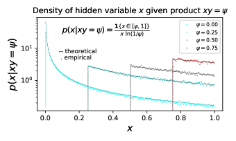
Figure 8: The probability density of the value of one member $x$ of a product $xy$ conditioned on $xy=\psi$. In the absence of the conditionality, both $x$ and $y$ are distributed uniformly on $[0,1]$.

C.2 Finding $p_{1}(\phi|\psi)$

Now suppose that one variable, say $y$, undergoes a random jump (i.e., is resampled) and thus becomes a new uniform variable on $[0,1]$. The equality $xy=\psi$ no longer holds, but since it did hold prior to the jump, the variable $x$ remains distributed according to $p(x|xy=\psi)$. Therefore the new product’s value, which we denote by $\phi=xy^{\prime}$ (where $y^{\prime}$ is the post-jump version of $y$), has a density $p_{1}(\phi|\psi)$ of the following form:

$$p_{1}(\phi|\psi) =\int_{0}^{1}\mathbf{1}\{y^{\prime}\in[0,1]\}p\left(\left.\frac{\phi}{y^{\prime}}\right|xy=\psi\right)\frac{1}{y^{\prime}}dy^{\prime}$$ (62)

$$=\int_{0}^{1}\frac{\mathbf{1}\{\phi/y^{\prime}\in[\psi,1]\}}{(\phi/y^{\prime})\ln(1/\psi)}\frac{dy^{\prime}}{y^{\prime}}$$

$$=\frac{1}{\phi\ln(1/\psi)}\int_{0}^{1}\mathbf{1}\{\phi/y^{\prime}\in[\psi,1]\}dy^{\prime}.$$

Continuing with a change of variables,

$$p_{1}(\phi|\psi) =\frac{1}{\ln(1/\psi)}\int_{0}^{1/\phi}\mathbf{1}\{y^{\prime}/\phi\in[1,1/\psi]\}d(y^{\prime}/\phi)$$ (63)

$$=\frac{\min(1/\phi,1/\psi)-1}{\ln(1/\psi)}.$$

The above is validated numerically in Figure 9.

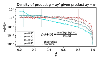
Figure 9: The probability density of the value $\phi$ of the product $\phi=xy^{\prime}$, where $y^{\prime}$ is uniformly sampled after having previously had random value $y$, and where $xy$ was conditioned to have value $xy=\psi$. Without any conditioning, all three $x,y,y^{\prime}$ have marginal density uniform on $[0,1]$.

C.3 Calculating $\bar{f}_{1}(\psi)$

We now average the affinity over $p_{1}(\phi|\psi)$, to get the contribution to the effective connection probability coming from one hidden variable jumping. This goes as

$$\bar{f}_{1}(\psi) =\int_{0}^{1}f(\phi)p_{1}(\phi|\psi)d\phi$$ (64)

$$=\int_{0}^{1}f(\phi)\frac{\min(1/\phi,1/\psi)-1}{\ln(1/\psi)}d\phi$$

$$=\frac{1}{\ln(1/\psi)}\left(\frac{1}{\psi}\int_{0}^{\psi}f(\phi)d\phi+\int_{\psi}^{1}\frac{f(\phi)}{\phi}d\phi-1\right).$$

Using Equation 64, we can compute the effective connection probability $\bar{f}(\psi)$ for a given affinity-function $f(\psi)$ via Equation 56.

Appendix D Walk-Dynamics

Here we describe walk-dynamics in detail. Throughout this work, walk-dynamics in $1D$ is simulated by first mapping random variables to the unit interval (by the inverse-CDF method Devroye (2006)), doing a random walk on $[0,1]$, then mapping back. For any one-dimensional probability density $\nu(x)$ where $x\in\mathbb{R}_{+}$, we define random variable $u(x)=F_{\nu}(x)$, where $F_{\nu}(x)=\int_{0}^{x}\nu(y)dy$. The probability density of $u(x)$ is the uniform on $[0,1]$. A random walk on $[0,1]$ is constructed via addition of uniform noise in the range $[-2\sigma,2\sigma]$, parameterized by $\sigma\in[0,1]$. That is, after rescaling we have hidden-variable dynamics

$$\mathcal{P}_{h}(u^{\prime}|u)=\frac{\mathbf{1}\left\{|u^{\prime}-u|\leq 2\sigma\right\}}{4\sigma}.$$ (65)

Note that the choice of $[-2\sigma,2\sigma]$ results in a mean jump-length parameterized by $\sigma$:

$$\langle|u-u^{\prime}|\rangle =\int|u-u^{\prime}|\mathcal{P}_{h}(u^{\prime}|u)du^{\prime}$$ (66)

$$=\frac{1}{4\sigma}\int_{-2\sigma}^{2\sigma}|x|dx=\sigma$$

where boundary conditions have been neglected in the above case; when implementing boundary conditions, one needs only to adjust the probability density $\mathcal{P}_{h}(u^{\prime}|u)$ according to the circumstance. See Appendix E for the case of reflecting boundaries.

Drawing $h^{(1)}$ from $\nu$, we initialize $u^{(1)}=F_{\nu}(h^{(1)})$ and iteratively time-advance as per the above to obtain $\{u^{(t)}\}_{t=1}^{T}$. We then simply transform back via $h^{(t)}=F_{\nu}^{-1}(u^{(t)})$, to obtain one-dimensional dynamics whose stationary distribution is $\nu$.

In dimensions greater than $1$, walk-dynamics can be simulated by first taking the multidimensional inverse-CDF transform, mapping the space $\mathcal{X}$ to a unit cube. Walk-dynamics can then be performed with whatever custom boundary conditions are required on that unit cube (boundary conditions that correspond to those of $\mathcal{X}$), and the results can then be mapped back to the original space $\mathcal{X}$. For example in the $\mathbb{H}^{2}$ model (Appendix F), increments of change in the angular and radial coordinates were chosen to be independent; this option was taken for simplicity, but non-independent cases would also be interesting to explore. Any transitional probability density preserving the uniform on the unit cube would fall within the same framework.

Appendix E Walk-dynamics with reflecting boundary conditions

In this appendix we study walk-dynamics on $\mathcal{X}=[0,1]$ with reflecting boundary conditions under uniform noise. In particular, we show that the stationary density is uniform on $[0,1]$. In turn, that implies that arbitrary 1D dynamics with density $\nu(h)$ can be made into a random walk of this type, by mapping initial $h$-values to $[0,1]$ via the inverse-CDF transform, performing the reflecting random walk on $[0,1]$, then transforming the random walk trajectories back to the original space (see appendix D).

Let $\mathcal{X}=[0,1]$ be the HV-space and denote by $x\hookleftarrow U[0,1]$ the value of a hidden variable. Then let $\hat{x}\in[-r,1+r]$ be an intermediate variable defined as $\hat{x}=x+u$, where $u\hookleftarrow U[-r,r]$ is the uniform additive noise which we use to simulate walk-dynamics. Lastly, let $x^{\prime}=Z(\hat{x})$ be the reflected variable, where the function $Z$ encodes the reflecting boundary conditions. Note that values of $x^{\prime}$ in the ranges $[0,r]$ and $[1-r,1]$ are obtained from one of two different of values of $\hat{x}$: the case when reflected, and the case when not reflected. To transform the density of $\hat{x}$ into that of $x^{\prime}$, we write $x^{\prime}$ as a function of $\hat{z}$, as $x^{\prime}=Z(\hat{x})$ and use the generalized change-of-variables formula for probability densities Billingsley (2008). We denote the densities of $x,\hat{x},x^{\prime}$ as $P(x),\hat{P}(\hat{x})$, and $P^{\prime}(x^{\prime})$, respectively. Then we have the following:

$$P(x^{\prime})=\sum_{\hat{x}:Z(\hat{x})=x^{\prime}}\left|\frac{dZ(\hat{x})}{d\hat{x}}\right|^{-1}P(\hat{x}),$$ (67)

by the rules of how probabilities densities transform Billingsley (2008). The density of $\hat{x}$ given $x$ is

$$\hat{P}(\hat{x}|x)=\frac{\mathbf{1}\{\hat{x}\in[x-r,x+r]\}}{2r}=\frac{\mathbf{1}\{x\in[\hat{x}-r,\hat{x}+r]\}}{2r}.$$ (68)

Since $x$ is uniform on $[0,1]$ the density of $\hat{x}$ is then

$$\hat{P}(\hat{x}) =\int_{0}^{1}\hat{P}(\hat{x}|x)dx$$ (69)

$$=\frac{1}{2r}\int_{0}^{1}\mathbf{1}\{x\in[\hat{x}-r,\hat{x}+r]\}dx$$

$$=\frac{1}{2r}\left|[0,1]\cup[\hat{x}-r,\hat{x}+r]\right|,$$

or

$$\hat{P}(\hat{x})=\frac{1}{2r}\left\{\begin{array}[]{cc}\hat{x}+r,&\hat{x}<r,\\ 2r&\hat{x}\in[r,1-r],\\ 1+r-\hat{x},&\hat{x}>1-r.\end{array}\right.$$ (70)

where the $\hat{x}$-dependent coefficients of the first and third terms arise from reflections of the form $\hat{x}-(-r)$ and $1-(\hat{x}-1)$. We seek a function $Z:[-r,1+r]\rightarrow[0,1]$ that encodes the reflection properties of the walk-dynamics. The necessary $Z$ is given by

$$Z(\hat{x}) =\left\{\begin{array}[]{cc}-\hat{x},&\hat{x}<0,\\ \hat{x},&\hat{x}\in[0,1],\\ 2-\hat{x},&\hat{x}>1.\end{array}\right.$$ (71)

The values of $\hat{x}$ mapping to a given value of $x^{\prime}$, namely those making up the inverse of $Z$, are given by

$$\{\hat{x}:Z(\hat{x})=x^{\prime}\}=\left\{\begin{array}[]{cc}\{-x^{\prime},x^{\prime}\},&x^{\prime}<r,\\ \{x^{\prime}\},&x^{\prime}\in[r,1-r],\\ \{x^{\prime},2-x^{\prime}\},&x^{\prime}>1-r.\\ \end{array}\right.$$ (72)

Let us compute the derivative of $Z(\hat{x})$, neglecting the measure-zero points of $0$ and $1$:

$$\frac{dZ(\hat{x})}{d\hat{x}}=\left\{\begin{array}[]{cc}-1,&\hat{x}<0,\\ 1,&\hat{x}\in(0,1),\\ -1,&\hat{x}>1.\end{array}\right.$$ (73)

We now transform to find the density after one step of dynamics, as

$$P^{\prime}(x^{\prime}) =\sum_{\hat{x}:Z(\hat{x})=x^{\prime}}\left|\frac{dZ(\hat{x})}{d\hat{x}}\right|^{-1}\hat{P}(\hat{x})$$ (74)

$$=\left\{\begin{array}[]{cc}\hat{P}(-x^{\prime})+\hat{P}(x^{\prime}),&x^{\prime}<r,\\ \hat{P}(x^{\prime}),&x^{\prime}\in[r,1-r],\\ \hat{P}(x^{\prime})+\hat{P}(2-x^{\prime}),&x^{\prime}>1-r.\\ \end{array}\right.$$

$$=\frac{1}{2r}\left\{\begin{array}[]{cc}2r,&x^{\prime}<r,\\ 2r,&x^{\prime}\in[r,1-r],\\ 2r,&x^{\prime}>1-r.\\ \end{array}\right.$$

$$=1.$$

Therefore, $P^{\prime}(x^{\prime})=1$ for all $x^{\prime}\in[0,1]$, and thus the uniform distribution is the stationary distribution of reflecting walk-dynamics.

Appendix F Hyperbolic walk-dynamics

To sample $\tilde{h}=(\tilde{r},\tilde{\theta})$, and also to sample $h_{j}^{(1)}$ (a coordinate from the initial timestep, i.e. the static $\mathbb{H}^{2}$ model), we first draw two independent random variables $U_{r}$ and $U_{\theta}$, each from the uniform distribution on $[0,1]$. These are then set equal to the cumulative density functions of $\nu_{rad}$ and $\nu_{ang}$, evaluated at $\tilde{r}$ and $\tilde{\theta}$, respectively:

$$U_{\theta} =\int_{0}^{\tilde{\theta}}\nu_{ang}(\theta)d\theta=\frac{\tilde{\theta}}{2\pi},$$ (75)

$$U_{r} =\int_{0}^{\tilde{r}}\nu_{rad}(r)dr=\frac{\cosh\left(\frac{\gamma-1}{2}\tilde{r}\right)-1}{\cosh\left(\frac{\gamma-1}{2}R\right)-1}.$$

From the above, we can solve to obtain $\tilde{h}$ in terms of $(U_{r},U_{\theta})$:

$$\tilde{\theta} =2\pi U_{\theta},$$ (76)

$$\tilde{r} =\frac{2}{\gamma-1}\cosh^{-1}\left(1+\left(\cosh\left(\frac{\gamma-1}{2}R\right)-1\right)U_{r}\right).$$

In the temporal setting, those initial variables are set to $U^{(1)}_{\theta}$ and $U^{(1)}_{r}$, after which we perform walk dynamics on the transformed variables to obtain $(U^{(t)}_{\theta},U^{(t)}_{r})$ for $t\in\{2,...,T\}$. Walk-dynamics occurs independently for the two variables, with periodic boundary conditions for angular coordinates and reflecting boundary conditions for radial coordinates.

Note that we use reflecting boundary conditions for the radial coordinate, rather than, for example, periodic boundary conditions, or reflecting boundary conditions with an associated angular reversal at any timestep that a node reflects from the origin of the radial coordinate (as would also seem like a natural choice for the disk). The reason to not incorporate such angular flipping is due to the interpretation of the angular coordinates as similarity-encoding variables Papadopoulos et al. (2012). From that perspective, it is more realistic to have nodes reflect off of the disk’s origin and retain their similarity-coordinates, rather than to pass through the origin and reverse their similarity-coordinates.

Appendix G Stationarity with Link-Response

In this appendix, we show that the static-model graph probability distribution is preserved via the effect of link-response as described in Section VI. Specifically, we show that

$$\int_{\mathcal{H}}\left(\sum_{G\in\mathcal{G}}\mathbb{P}(G|H)P^{G\rightarrow G^{\prime}}_{H,H^{\prime}}\right)\rho(H)dH=\mathbb{P}(G^{\prime}|H^{\prime}),$$ (77)

where $P^{G^{(t)}\rightarrow G^{(t+1)}}_{H^{(t)},H^{(t+1)}}=\mathcal{P}_{G}(G^{(t+1)}|G^{(t)},H^{(t+1)},H^{(t)})$. We for now set $\omega=0$ and later argue that link-resampling does not influence the results in question. First, we note that the transition probability given $(H,H^{\prime})$ is separable: $P^{G\rightarrow G^{\prime}}_{H,H^{\prime}}=\prod_{1\leq i<j\leq n}P_{ij}^{A_{ij}\rightarrow A_{ij}^{\prime}}$, with transition probability $P_{ij}^{\alpha\rightarrow\beta}=\mathbb{P}(A_{ij}^{\prime}=\beta|A_{ij}=\alpha,h_{i}^{\prime},h_{j}^{\prime},h_{i},h_{j})$. Denoting $f_{ij}=f(h_{i},h_{j})$ and $f^{\prime}_{ij}=f(h^{\prime}_{i},h^{\prime}_{j})$, we evaluate the different transition probabilities:

$$P_{ij}^{1\rightarrow 1} =\mathbf{1}\left\{f_{ij}^{\prime}\geq f_{ij}\right\}+(1-q^{-}_{ij})\mathbf{1}\{f_{ij}^{\prime}<f_{ij}\},$$ (78)

$$P_{ij}^{0\rightarrow 0} =\mathbf{1}\left\{f_{ij}^{\prime}<f_{ij}\right\}+(1-q^{+}_{ij})\mathbf{1}\{f_{ij}^{\prime}\geq f_{ij}\},$$

with $q^{-}_{ij}=1-f^{\prime}_{ij}/f_{ij}$, $q^{+}_{ij}=1-(1-f^{\prime}_{ij})/(1-f_{ij})$ as defined in Section VI. The remaining probabilities are obtained by normalization:

$$P_{ij}^{1\rightarrow 0} =1-P_{ij}^{1\rightarrow 1}=q^{-}_{ij}\mathbf{1}\left\{f_{ij}^{\prime}<f_{ij}\right\},$$ (79)

$$P_{ij}^{0\rightarrow 1} =1-P_{ij}^{0\rightarrow 0}=q^{+}_{ij}\mathbf{1}\left\{f_{ij}^{\prime}\geq f_{ij}\right\}.$$

Noting that $P^{G\rightarrow G^{\prime}}_{H,H^{\prime}}$ and $\mathbb{P}(G|H)$ are both separable into a product over $ij:1\leq i<j\leq n$, we write

$$\mathbb{P}(G|H)P^{G\rightarrow G^{\prime}}_{H,H^{\prime}}=\prod_{1\leq i<j\leq n}f_{ij}^{A_{ij}}(1-f_{ij})^{1-A_{ij}}P_{ij}^{A_{ij}\rightarrow A_{ij}^{\prime}}.$$ (80)

The sum over all graphs $G$ of this product becomes a product over all pairs $ij$ of a sum over $A_{ij}\in\{0,1\}$:

$$\sum_{G\in\mathcal{G}}\prod_{1\leq i<j\leq n}y(A_{ij})=\prod_{1\leq i<j\leq n}\sum_{A_{ij}\in\{0,1\}}y(A_{ij}).$$ (81)

Using the above, and the static-model graph probability distribution (Equation 5), the parenthesized term in Equation 77 is equal to

$$\prod_{ij:A_{ij}^{\prime}=0}\left(f_{ij}P_{ij}^{1\rightarrow 0}+(1-f_{ij})P_{ij}^{0\rightarrow 0}\right)$$ (82)

$$\times \prod_{ij:A_{ij}^{\prime}=1}\left(f_{ij}P_{ij}^{1\rightarrow 1}+(1-f_{ij})P_{ij}^{0\rightarrow 1}\right).$$

Applying equations (78, 79) and using the expressions for $q^{\pm}_{ij}$, as well as the facts that $\mathbf{1}\{f^{\prime}_{ij}\geq f_{ij}\}+\mathbf{1}\{f^{\prime}_{ij}<f_{ij}\}=1$ and $\int_{\mathcal{H}}\rho(H)dH=1$, Equation 77 becomes

$$\prod_{ij:A_{ij}^{\prime}=1}f^{\prime}_{ij}\prod_{ij:A_{ij}^{\prime}=0}(1-f^{\prime}_{ij})=\mathbb{P}(G^{\prime}|H^{\prime}).$$ (83)

The left-hand side of the above is exactly the static model’s graph probability distribution given a hidden-variable configuration (see Equation 5 of the main text). Thus the static hidden-variables model is the stationary distribution of time-advancements with the link-response mechanism.

To show that these results hold even upon inclusion of the link-resampling mechanism (allowing $\omega>0$), consider the following reasoning. Regardless of what the link-response step yielded, each node-pair undergoing link-resampling at rate $\omega$ will result in either (a) linking according to the connection probability of the newly updated hidden-variable configuration (with probability $\omega$) or (b) linking as before ($\omega=0$), without altering the connection probability. Given the fact that stationarity holds without link-resampling, in the latter case we also have a connection probability equal to that of the updated hidden-variable configuration.

Thus, upon inclusion of the link-response mechanism whereby both $H^{(t+1)}$ and $H^{(t)}$ impact the transition from $G^{(t)}$ to $G^{(t+1)}$, we have temporal extensions of arbitrary static hidden-variables models that exactly satisfy the Equilibrium property, while retaining the Persistence Property. Such a link-response mechanism may better reflect reality in cases where connectivity among nodes changes directly in response to changes in their internal characteristics.

Appendix H Discrete hidden variables

We consider THVMs formulated with discrete hidden variables, and describe their relation to continous-HV models.

We take for example the case of SBMs, described in Section V.1 entirely in terms of discrete HVs, namely group-indices which are naturally thought of as discrete. We then have a set of discrete HVs $\{q_{j}\}_{j\in[n]}$, each distributed into a discrete set $[m]=\{1,...,m\}$ according to a probability distribution $\varrho:[m]\rightarrow[0,1]$, and connecting via a discrete affinity-function $f_{q,q^{\prime}}$.

In a dual continuous-HV system which maps to the above-described discrete system, suppose each node $j$’s hidden variable $h_{j}$ has uniform density on $[0,1]$, and pairwise affinities are encoded in a piecewise constant graphon function according to occupancy of points in nonoverlapping subregions $\{L_{w}\}_{w\in[m]}\subseteq[0,1]^{m}$ such that $|L_{w}|=\varrho_{w}$ and such that

$$f(h,h^{\prime})=\sum_{(w,z)\in[m]^{2}}f_{w,z}\mathbf{1}\{h\in L_{w},h^{\prime}\in L_{z}\}.$$ (84)

Discrete node-labels can also be written directly in terms of continuous HV-values, as

$$q_{i}=\sum_{q\in[m]}q\mathbf{1}\{h_{i}\in L_{q}\}.$$ (85)

The probability distribution $\varrho$ thus arises from integration of the uniform density on $[0,1]$, namely $\nu(h)=1$, over the regions $\{L_{q}\}_{q\in[m]}$ corresponding to specific group-labels $q\in[m]$:

$$\varrho_{q}=\int_{\mathcal{X}}\nu(h)\mathbf{1}\{h\in L_{q}\}dh=\int_{L_{q}}dh=|L_{q}|.$$ (86)

In the temporal setting, we can again relate discrete HVs to continuous ones. To reproduce the HV-resampling dynamics for temporal SBMs, we can simply have continuous HVs undergo jump-dynamics in $[0,1]$. Jumping to a random point in $[0,1]$ amounts to jumping into a random subset $L_{q}$ with probability $\varrho_{q}=|L_{q}|$.

References

- Janwa et al. (2019) Heeralal Janwa, Steven Massey, Julian Velev, and Bud Bhubaneswar Mishra, “On the origin of biomolecular networks,” Frontiers in genetics 10, 240 (2019).
- Boers et al. (2019) Niklas Boers, Bedartha Goswami, Aljoscha Rheinwalt, Bodo Bookhagen, Brian Hoskins, and Jürgen Kurths, “Complex networks reveal global pattern of extreme-rainfall teleconnections,” Nature 566, 373 (2019).
- Costa et al. (2011) Luciano da Fontoura Costa, Osvaldo N Oliveira Jr, Gonzalo Travieso, Francisco Aparecido Rodrigues, Paulino Ribeiro Villas Boas, Lucas Antiqueira, Matheus Palhares Viana, and Luis Enrique Correa Rocha, “Analyzing and modeling real-world phenomena with complex networks: a survey of applications,” Advances in Physics 60, 329–412 (2011).
- Rocha et al. (2010) Luis EC Rocha, Fredrik Liljeros, and Petter Holme, “Information dynamics shape the sexual networks of internet-mediated prostitution,” Proceedings of the National Academy of Sciences 107, 5706–5711 (2010).
- West et al. (1997) Geoffrey B West, James H Brown, and Brian J Enquist, “A general model for the origin of allometric scaling laws in biology,” Science 276, 122–126 (1997).
- Pastor-Satorras and Vespignani (2004) Romualdo Pastor-Satorras and Alessandro Vespignani, Evolution and structure of the Internet: A statistical physics approach (Cambridge University Press, 2004).
- Zheng et al. (2020) Muhua Zheng, Antoine Allard, Patric Hagmann, Yasser Alemán-Gómez, and M Ángeles Serrano, “Geometric renormalization unravels self-similarity of the multiscale human connectome,” Proceedings of the National Academy of Sciences 117, 20244–20253 (2020).
- Cimini et al. (2019) Giulio Cimini, Tiziano Squartini, Fabio Saracco, Diego Garlaschelli, Andrea Gabrielli, and Guido Caldarelli, “The statistical physics of real-world networks,” Nature Reviews Physics 1, 58–71 (2019).
- Kim et al. (2019) Hyunju Kim, Harrison B Smith, Cole Mathis, Jason Raymond, and Sara I Walker, “Universal scaling across biochemical networks on earth,” Science advances 5, eaau0149 (2019).
- Krapivsky and Redner (2002) Paul L Krapivsky and Sidney Redner, “A statistical physics perspective on web growth,” Computer Networks 39, 261–276 (2002).
- Barabási and Albert (1999) Albert-László Barabási and Réka Albert, “Emergence of scaling in random networks,” science 286, 509–512 (1999).
- Bianconi and Barabási (2001) Ginestra Bianconi and A-L Barabási, “Competition and multiscaling in evolving networks,” EPL (Europhysics Letters) 54, 436 (2001).
- Caldarelli et al. (2002) Guido Caldarelli, Andrea Capocci, Paolo De Los Rios, and Miguel A Munoz, “Scale-free networks from varying vertex intrinsic fitness,” Physical review letters 89, 258702 (2002).
- Barthelemy (2018) Marc Barthelemy, Morphogenesis of spatial networks (Springer, 2018).
- Krioukov et al. (2010) Dmitri Krioukov, Fragkiskos Papadopoulos, Maksim Kitsak, Amin Vahdat, and Marián Boguná, “Hyperbolic geometry of complex networks,” Physical Review E 82, 036106 (2010).
- Serrano et al. (2012) M Ángeles Serrano, Marián Boguná, and Francesc Sagués, “Uncovering the hidden geometry behind metabolic networks,” Molecular biosystems 8, 843–850 (2012).
- Kitsak et al. (2017) Maksim Kitsak, Fragkiskos Papadopoulos, and Dmitri Krioukov, “Latent geometry of bipartite networks,” Physical Review E 95, 032309 (2017).
- Boguná and Pastor-Satorras (2003) Marián Boguná and Romualdo Pastor-Satorras, “Class of correlated random networks with hidden variables,” Physical Review E 68, 036112 (2003).
- Newman (2018) Mark Newman, Networks (Oxford university press, 2018).
- Karrer and Newman (2011) Brian Karrer and Mark EJ Newman, “Stochastic blockmodels and community structure in networks,” Physical review E 83, 016107 (2011).
- Penrose et al. (2003) Mathew Penrose et al., Random geometric graphs, Vol. 5 (Oxford university press, 2003).
- van der Hoorn et al. (2018) Pim van der Hoorn, Gabor Lippner, and Dmitri Krioukov, “Sparse maximum-entropy random graphs with a given power-law degree distribution,” Journal of Statistical Physics 173, 806–844 (2018).
- Risau-Gusmán and Zanette (2009) Sebastián Risau-Gusmán and Damián H Zanette, “Contact switching as a control strategy for epidemic outbreaks,” Journal of theoretical biology 257, 52–60 (2009).
- Piankoranee and Limkumnerd (2018) Suwakan Piankoranee and Surachate Limkumnerd, “Effects of global and local rewiring on sis epidemic adaptive networks,” in Journal of Physics: Conference Series, Vol. 1144 (IOP Publishing, 2018) p. 012080.
- Huepe et al. (2011) Cristián Huepe, Gerd Zschaler, Anne-Ly Do, and Thilo Gross, “Adaptive-network models of swarm dynamics,” New Journal of Physics 13, 073022 (2011).
- Marceau et al. (2010) Vincent Marceau, Pierre-André Noël, Laurent Hébert-Dufresne, Antoine Allard, and Louis J Dubé, “Adaptive networks: Coevolution of disease and topology,” Physical Review E 82, 036116 (2010).
- Demirel et al. (2014) Guven Demirel, Federico Vazquez, GA Böhme, and Thilo Gross, “Moment-closure approximations for discrete adaptive networks,” Physica D: Nonlinear Phenomena 267, 68–80 (2014).
- Gross and Sayama (2009) Thilo Gross and Hiroki Sayama, “Adaptive networks,” in Adaptive networks (Springer, 2009) pp. 1–8.
- Crabtree and Soltysiak (1998) I Barry Crabtree and Stuart J Soltysiak, “Identifying and tracking changing interests,” International Journal on Digital Libraries 2, 38–53 (1998).
- Chapman et al. (2011) Ben B Chapman, Christer Brönmark, Jan-Åke Nilsson, and Lars-Anders Hansson, “The ecology and evolution of partial migration,” Oikos 120, 1764–1775 (2011).
- Vardanis et al. (2011) Yannis Vardanis, Raymond HG Klaassen, Roine Strandberg, and Thomas Alerstam, “Individuality in bird migration: routes and timing,” Biology letters 7, 502–505 (2011).
- Altizer et al. (2011) Sonia Altizer, Rebecca Bartel, and Barbara A Han, “Animal migration and infectious disease risk,” science 331, 296–302 (2011).
- Pfeffer and Dobler (2010) Martin Pfeffer and Gerhard Dobler, “Emergence of zoonotic arboviruses by animal trade and migration,” Parasites & vectors 3, 35 (2010).
- Hein et al. (2012) Andrew M Hein, Chen Hou, and James F Gillooly, “Energetic and biomechanical constraints on animal migration distance,” Ecology letters 15, 104–110 (2012).
- Carroll et al. (2007) Scott P Carroll, Andrew P Hendry, David N Reznick, and Charles W Fox, “Evolution on ecological time-scales,” Functional Ecology 21, 387–393 (2007).
- Held et al. (2014) Torsten Held, Armita Nourmohammad, and Michael Lässig, “Adaptive evolution of molecular phenotypes,” Journal of Statistical Mechanics: Theory and Experiment 2014, P09029 (2014).
- Volberda and Lewin (2003) Henk W Volberda and Arie Y Lewin, “Co-evolutionary dynamics within and between firms: From evolution to co-evolution,” Journal of management studies 40, 2111–2136 (2003).
- Stoica and Schindehutte (1999) Michael Stoica and Minet Schindehutte, “Understanding adaptation in small firms: Links to culture and performance,” Journal of Developmental Entrepreneurship 4, 1 (1999).
- Johnson (2006) Kenneth M Johnson, “Demographic trends in rural and small town america,” (2006), 10.34051/p/2020.6.
- Myers (1999) Dowell Myers, “Demographic dynamism and metropolitan change: Comparing los angeles, new york, chicago, and washington, dc,” Housing Policy Debate 10, 919–954 (1999).
- Raimbault (2018) Juste Raimbault, “Modeling the co-evolution of cities and networks,” arXiv preprint arXiv:1804.09430 (2018).
- Kuhar et al. (1993) Siobhan G Kuhar, Lei Feng, Susana Vidan, M Elizabeth Ross, Mary E Hatten, and Nathaniel Heintz, “Changing patterns of gene expression define four stages of cerebellar granule neuron differentiation,” Development 117, 97–104 (1993).
- McCormack et al. (1992) Matthew A McCormack, Kenneth M Rosen, Lydia Villa-Komaroff, and George D Mower, “Changes in immediate early gene expression during postnatal development of cat cortex and cerebellum,” Molecular brain research 12, 215–223 (1992).
- Dalvand et al. (2008) Mohammad Moradi Dalvand, Seyed Bahram Zahir Azami, and Hadi Tarimoradi, “Long-term load forecasting of iranian power grid using fuzzy and artificial neural networks,” in 2008 43rd International Universities Power Engineering Conference (IEEE, 2008) pp. 1–4.
- De Felice et al. (2013) Matteo De Felice, Andrea Alessandri, and Paolo M Ruti, “Electricity demand forecasting over italy: Potential benefits using numerical weather prediction models,” Electric Power Systems Research 104, 71–79 (2013).
- Pasichnyk et al. (2014) Natalia Pasichnyk, Mykola Dyvak, and Roman Pasichnyk, “Mathematical modeling of website quality characteristics in dynamics,” in Journal of Applied Computer Science, Vol. 22 (Technical University Press, 2014) pp. 171–183.
- Bean (2011) Sandra J Bean, “Emerging and continuing trends in vaccine opposition website content,” Vaccine 29, 1874–1880 (2011).
- Nicosia et al. (2013) Vincenzo Nicosia, John Tang, Cecilia Mascolo, Mirco Musolesi, Giovanni Russo, and Vito Latora, “Graph metrics for temporal networks,” in Temporal networks (Springer, 2013) pp. 15–40.
- Ortiz et al. (2017) Elisenda Ortiz, Michele Starnini, and M Ángeles Serrano, “Navigability of temporal networks in hyperbolic space,” Scientific reports 7, 15054 (2017).
- Taylor et al. (2017) Dane Taylor, Sean A Myers, Aaron Clauset, Mason A Porter, and Peter J Mucha, “Eigenvector-based centrality measures for temporal networks,” Multiscale Modeling & Simulation 15, 537–574 (2017).
- Kim and Anderson (2012) Hyoungshick Kim and Ross Anderson, “Temporal node centrality in complex networks,” Physical Review E 85, 026107 (2012).
- Pan and Saramäki (2011) Raj Kumar Pan and Jari Saramäki, “Path lengths, correlations, and centrality in temporal networks,” Physical Review E 84, 016105 (2011).
- Li et al. (2017) Aming Li, Sean P Cornelius, Y-Y Liu, Long Wang, and A-L Barabási, “The fundamental advantages of temporal networks,” Science 358, 1042–1046 (2017).
- Liu et al. (2014) Suyu Liu, Nicola Perra, Márton Karsai, and Alessandro Vespignani, “Controlling contagion processes in activity driven networks,” Physical review letters 112, 118702 (2014).
- Perra et al. (2012a) Nicola Perra, Andrea Baronchelli, Delia Mocanu, Bruno Gonçalves, Romualdo Pastor-Satorras, and Alessandro Vespignani, “Random walks and search in time-varying networks,” Physical review letters 109, 238701 (2012a).
- Paranjape et al. (2017) Ashwin Paranjape, Austin R Benson, and Jure Leskovec, “Motifs in temporal networks,” in Proceedings of the Tenth ACM International Conference on Web Search and Data Mining (ACM, 2017) pp. 601–610.
- Holme (2016) Petter Holme, “Temporal network structures controlling disease spreading,” Physical Review E 94, 022305 (2016).
- Liu et al. (2018) Quan-Hui Liu, Xinyue Xiong, Qian Zhang, and Nicola Perra, “Epidemic spreading on time-varying multiplex networks,” Physical Review E 98, 062303 (2018).
- Nadini et al. (2018) Matthieu Nadini, Kaiyuan Sun, Enrico Ubaldi, Michele Starnini, Alessandro Rizzo, and Nicola Perra, “Epidemic spreading in modular time-varying networks,” Scientific reports 8, 2352 (2018).
- Masuda and Holme (2017) Naoki Masuda and Petter Holme, Temporal network epidemiology (Springer, 2017).
- Sun et al. (2015) Kaiyuan Sun, Andrea Baronchelli, and Nicola Perra, “Contrasting effects of strong ties on sir and sis processes in temporal networks,” The European Physical Journal B 88, 326 (2015).
- Li et al. (2018) Dandan Li, Dun Han, Jing Ma, Mei Sun, Lixin Tian, Timothy Khouw, and H Eugene Stanley, “Opinion dynamics in activity-driven networks,” EPL (Europhysics Letters) 120, 28002 (2018).
- Dunlavy et al. (2011) Daniel M Dunlavy, Tamara G Kolda, and Evrim Acar, “Temporal link prediction using matrix and tensor factorizations,” ACM Transactions on Knowledge Discovery from Data (TKDD) 5, 10 (2011).
- Dhote et al. (2013) Yugchhaya Dhote, Nishchol Mishra, and Sanjeev Sharma, “Survey and analysis of temporal link prediction in online social networks,” in 2013 International Conference on Advances in Computing, Communications and Informatics (ICACCI) (IEEE, 2013) pp. 1178–1183.
- Sarzynska et al. (2016) Marta Sarzynska, Elizabeth A Leicht, Gerardo Chowell, and Mason A Porter, “Null models for community detection in spatially embedded, temporal networks,” Journal of Complex Networks 4, 363–406 (2016).
- Gauvin et al. (2014) Laetitia Gauvin, André Panisson, and Ciro Cattuto, “Detecting the community structure and activity patterns of temporal networks: a non-negative tensor factorization approach,” PloS one 9, e86028 (2014).
- Peixoto and Rosvall (2017) Tiago P Peixoto and Martin Rosvall, “Modelling sequences and temporal networks with dynamic community structures,” Nature communications 8, 582 (2017).
- Xu and Hero (2014) Kevin S Xu and Alfred O Hero, “Dynamic stochastic blockmodels for time-evolving social networks,” IEEE Journal of Selected Topics in Signal Processing 8, 552–562 (2014).
- Xu (2015) Kevin Xu, “Stochastic block transition models for dynamic networks,” in Artificial Intelligence and Statistics (2015) pp. 1079–1087.
- Matias and Miele (2017) Catherine Matias and Vincent Miele, “Statistical clustering of temporal networks through a dynamic stochastic block model,” Journal of the Royal Statistical Society: Series B (Statistical Methodology) 79, 1119–1141 (2017).
- Pensky et al. (2019) Marianna Pensky, Teng Zhang, et al., “Spectral clustering in the dynamic stochastic block model,” Electronic Journal of Statistics 13, 678–709 (2019).
- Ghasemian et al. (2016) Amir Ghasemian, Pan Zhang, Aaron Clauset, Cristopher Moore, and Leto Peel, “Detectability thresholds and optimal algorithms for community structure in dynamic networks,” Physical Review X 6, 031005 (2016).
- Barucca et al. (2018) Paolo Barucca, Fabrizio Lillo, Piero Mazzarisi, and Daniele Tantari, “Disentangling group and link persistence in dynamic stochastic block models,” Journal of Statistical Mechanics: Theory and Experiment 2018, 123407 (2018).
- Sewell and Chen (2016) Daniel K Sewell and Yuguo Chen, “Latent space models for dynamic networks with weighted edges,” Social Networks 44, 105–116 (2016).
- Kim et al. (2018) Bomin Kim, Kevin H Lee, Lingzhou Xue, and Xiaoyue Niu, “A review of dynamic network models with latent variables,” Statistics surveys 12, 105 (2018).
- Sarkar et al. (2007) Purnamrita Sarkar, Sajid M Siddiqi, and Geogrey J Gordon, “A latent space approach to dynamic embedding of co-occurrence data,” in Artificial Intelligence and Statistics (2007) pp. 420–427.
- Sarkar and Moore (2006) Purnamrita Sarkar and Andrew W Moore, “Dynamic social network analysis using latent space models,” in Advances in Neural Information Processing Systems (2006) pp. 1145–1152.
- Peres et al. (2013) Yuval Peres, Alistair Sinclair, Perla Sousi, and Alexandre Stauffer, “Mobile geometric graphs: Detection, coverage and percolation,” Probability Theory and Related Fields 156, 273–305 (2013).
- Clementi and Silvestri (2015) Andrea Clementi and Riccardo Silvestri, “Parsimonious flooding in geometric random-walks,” Journal of Computer and System Sciences 81, 219–233 (2015).
- Norris (1998) James R Norris, Markov chains, 2 (Cambridge university press, 1998).
- Behrends (2000) Ehrhard Behrends, Introduction to Markov chains, Vol. 228 (Springer, 2000).
- Bianconi (2018) Ginestra Bianconi, Multilayer networks: structure and function (Oxford university press, 2018).
- De Domenico et al. (2013) Manlio De Domenico, Albert Solé-Ribalta, Emanuele Cozzo, Mikko Kivelä, Yamir Moreno, Mason A Porter, Sergio Gómez, and Alex Arenas, “Mathematical formulation of multilayer networks,” Physical Review X 3, 041022 (2013).
- Landsberg (1956) Peter T Landsberg, “Foundations of thermodynamics,” Reviews of modern physics 28, 363 (1956).
- Perra et al. (2012b) Nicola Perra, Bruno Goncalves, Romualdo Pastor-Satorras, and Alessandro Vespignani, “Activity driven modeling of time varying networks,” Scientific Reports 2, 469 (2012b).
- Papadopoulos and Flores (2019) Fragkiskos Papadopoulos and Marco Antonio Rodríguez Flores, “Latent geometry and dynamics of proximity networks,” Physical Review E 100, 052313 (2019).
- Bollobás et al. (2007) Béla Bollobás, Svante Janson, and Oliver Riordan, “The phase transition in inhomogeneous random graphs,” Random Structures & Algorithms 31, 3–122 (2007).
- Oliveira (2009) Roberto Imbuzeiro Oliveira, “Concentration of the adjacency matrix and of the laplacian in random graphs with independent edges,” arXiv preprint arXiv:0911.0600 (2009).
- Lu and Peng (2012) Linyuan Lu and Xing Peng, “Spectra of edge-independent random graphs,” arXiv preprint arXiv:1204.6207 (2012).
- Erdos and Renyi (1959) Paul Erdos and Alfred Renyi, “On random graphs i,” Publ. math. debrecen 6, 18 (1959).
- Anderson et al. (1992) Carolyn J Anderson, Stanley Wasserman, and Katherine Faust, “Building stochastic blockmodels,” Social networks 14, 137–161 (1992).
- Hartle et al. (2020) Harrison Hartle, Brennan Klein, Stefan McCabe, Alexander Daniels, Guillaume St-Onge, Charles Murphy, and Laurent Hébert-Dufresne, “Network comparison and the within-ensemble graph distance,” Proceedings of the Royal Society A 476, 20190744 (2020).
- Hamming (1950) Richard W Hamming, “Error detecting and error correcting codes,” The Bell system technical journal 29, 147–160 (1950).
- Steif (2009) Jeffrey E Steif, “A survey of dynamical percolation,” in Fractal geometry and stochastics IV (Springer, 2009) pp. 145–174.
- Peres and Steif (1998) Yuval Peres and Jeffrey E Steif, “The number of infinite clusters in dynamical percolation,” Probability theory and related fields 111, 141–165 (1998).
- Khoshnevisan (2008) Davar Khoshnevisan, “Dynamical percolation on general trees,” Probability theory and related fields 140, 169–193 (2008).
- Roberts et al. (2018) Matthew I Roberts, Batı Şengül, et al., “Exceptional times of the critical dynamical erdős–rényi graph,” The Annals of Applied Probability 28, 2275–2308 (2018).
- Rossignol (2020) Raphaël Rossignol, “Scaling limit of dynamical percolation on critical erdös-rényi random graphs,” arXiv preprint arXiv:1710.09101 (2020).
- Clementi et al. (2010) Andrea EF Clementi, Claudio Macci, Angelo Monti, Francesco Pasquale, and Riccardo Silvestri, “Flooding time of edge-markovian evolving graphs,” SIAM journal on discrete mathematics 24, 1694–1712 (2010).
- Whitbeck et al. (2011) John Whitbeck, Vania Conan, and Marcelo Dias de Amorim, “Performance of opportunistic epidemic routing on edge-markovian dynamic graphs,” IEEE Transactions on communications 59, 1259–1263 (2011).
- de Pebeyre et al. (2013) Aurelie Faure de Pebeyre, Fabien Tarissan, and Julien Sopena, “On the relevance of the edge-markovian evolving graph model for real mobile networks,” in 2013 IFIP Wireless Days (WD) (IEEE, 2013) pp. 1–6.
- Peixoto (2012) Tiago P Peixoto, “Entropy of stochastic blockmodel ensembles,” Physical Review E 85, 056122 (2012).
- Peixoto (2017) Tiago P Peixoto, “Nonparametric bayesian inference of the microcanonical stochastic block model,” Physical Review E 95, 012317 (2017).
- Kobourov (2012) Stephen G Kobourov, “Spring embedders and force directed graph drawing algorithms,” arXiv preprint arXiv:1201.3011 (2012).
- Söderberg (2003) Bo Söderberg, “Random graphs with hidden color,” Physical Review E 68, 015102 (2003).
- Söderberg (2002) Bo Söderberg, “General formalism for inhomogeneous random graphs,” Physical review E 66, 066121 (2002).
- Allen-Perkins (2018) Alfonso Allen-Perkins, “Random spherical graphs,” Physical Review E 98, 032310 (2018).
- Watts and Strogatz (1998) Duncan J Watts and Steven H Strogatz, “Collective dynamics of ‘small-world’networks,” nature 393, 440–442 (1998).
- Buscarino et al. (2008) Arturo Buscarino, Luigi Fortuna, Mattia Frasca, and Vito Latora, “Disease spreading in populations of moving agents,” EPL (Europhysics Letters) 82, 38002 (2008).
- Penrose et al. (2016) Mathew D Penrose et al., “Connectivity of soft random geometric graphs,” The Annals of Applied Probability 26, 986–1028 (2016).
- Wilsher et al. (2020) Michael Wilsher, Carl P Dettmann, and Ayalvadi Ganesh, “Connectivity in one-dimensional soft random geometric graphs,” arXiv preprint arXiv:2007.06301 (2020).
- Kaiser and Hilgetag (2004) Marcus Kaiser and Claus C Hilgetag, “Spatial growth of real-world networks,” Physical Review E 69, 036103 (2004).
- Dettmann and Georgiou (2016) Carl P Dettmann and Orestis Georgiou, “Random geometric graphs with general connection functions,” Physical Review E 93, 032313 (2016).
- Voitalov et al. (2020) Ivan Voitalov, Pim van der Hoorn, Maksim Kitsak, Fragkiskos Papadopoulos, and Dmitri Krioukov, “Weighted hypersoft configuration model,” Physical Review Research 2, 043157 (2020).
- Chung and Lu (2002) Fan Chung and Linyuan Lu, “Connected components in random graphs with given expected degree sequences,” Annals of combinatorics 6, 125–145 (2002).
- Norros and Reittu (2006) Ilkka Norros and Hannu Reittu, “On a conditionally poissonian graph process,” Advances in Applied Probability 38, 59–75 (2006).
- Bringmann et al. (2016) Karl Bringmann, Ralph Keusch, and Johannes Lengler, “Average distance in a general class of scale-free networks with underlying geometry,” arXiv preprint arXiv:1602.05712 (2016).
- Friedrich and Krohmer (2018) Tobias Friedrich and Anton Krohmer, “On the diameter of hyperbolic random graphs,” SIAM Journal on Discrete Mathematics 32, 1314–1334 (2018).
- Faqeeh et al. (2018) Ali Faqeeh, Saeed Osat, and Filippo Radicchi, “Characterizing the analogy between hyperbolic embedding and community structure of complex networks,” Physical review letters 121, 098301 (2018).
- García-Pérez et al. (2018) Guillermo García-Pérez, Marián Boguñá, and M Ángeles Serrano, “Multiscale unfolding of real networks by geometric renormalization,” Nature Physics 14, 583–589 (2018).
- Kardar (2007) Mehran Kardar, Statistical physics of particles (Cambridge University Press, 2007).
- Zhang et al. (2017) Xiao Zhang, Cristopher Moore, and Mark EJ Newman, “Random graph models for dynamic networks,” The European Physical Journal B 90, 200 (2017).
- Mandjes et al. (2019) Michel Mandjes, Nicos Starreveld, René Bekker, and Peter Spreij, “Dynamic erdős-rényi graphs,” in Computing and Software Science (Springer, 2019) pp. 123–140.
- Clementi et al. (2009) Andrea EF Clementi, Francesco Pasquale, Angelo Monti, and Riccardo Silvestri, “Information spreading in stationary markovian evolving graphs,” in 2009 IEEE International Symposium on Parallel & Distributed Processing (IEEE, 2009) pp. 1–12.
- Du et al. (2016) Ruijie Du, Hanxing Wang, and Yunbin Fu, “Continuous-time independent edge-markovian random graph process,” Chinese Annals of Mathematics, Series B 37, 73–82 (2016).
- Lamprou et al. (2018) Ioannis Lamprou, Russell Martin, and Paul Spirakis, “Cover time in edge-uniform stochastically-evolving graphs,” Algorithms 11, 149 (2018).
- Zino et al. (2016) Lorenzo Zino, Alessandro Rizzo, and Maurizio Porfiri, “Continuous-time discrete-distribution theory for activity-driven networks,” Physical review letters 117, 228–302 (2016).
- Pozzana et al. (2017) Iacopo Pozzana, Kaiyuan Sun, and Nicola Perra, “Epidemic spreading on activity-driven networks with attractiveness,” Physical Review E 96, 042310 (2017).
- da Mata and Pastor-Satorras (2015) Angélica Sousa da Mata and Romualdo Pastor-Satorras, “Slow relaxation dynamics and aging in random walks on activity driven temporal networks,” The European Physical Journal B 88, 12 (2015).
- Alessandretti et al. (2017) Laura Alessandretti, Kaiyuan Sun, Andrea Baronchelli, and Nicola Perra, “Random walks on activity-driven networks with attractiveness,” Physical Review E 95, 052318 (2017).
- Rizzo and Porfiri (2016) Alessandro Rizzo and Maurizio Porfiri, “Innovation diffusion on time-varying activity driven networks,” The European Physical Journal B 89, 20 (2016).
- Starnini and Pastor-Satorras (2014) Michele Starnini and Romualdo Pastor-Satorras, “Temporal percolation in activity-driven networks,” Physical Review E 89, 032807 (2014).
- Silvescu and Honavar (2001) Adrian Silvescu and Vasant Honavar, “Temporal boolean network models of genetic networks and their inference from gene expression time series,” Complex systems 13, 61–78 (2001).
- Lebre et al. (2010) Sophie Lebre, Jennifer Becq, Frederic Devaux, Michael PH Stumpf, and Gaelle Lelandais, “Statistical inference of the time-varying structure of gene-regulation networks,” BMC systems biology 4, 130 (2010).
- Hanneke et al. (2010) Steve Hanneke, Wenjie Fu, Eric P Xing, et al., “Discrete temporal models of social networks,” Electronic Journal of Statistics 4, 585–605 (2010).
- Mellor (2019) Andrew Mellor, “Event graphs: Advances and applications of second-order time-unfolded temporal network models,” Advances in Complex Systems 22, 1950006 (2019).
- Miles (1970) Roger E Miles, “On the homogeneous planar poisson point process,” Mathematical Biosciences 6, 85–127 (1970).
- Møller and Waagepetersen (2007) Jesper Møller and Rasmus P Waagepetersen, “Modern statistics for spatial point processes,” Scandinavian Journal of Statistics 34, 643–684 (2007).
- Reitzner (2013) Matthias Reitzner, “Poisson point processes: large deviation inequalities for the convex distance,” (2013), 10.1214/ecp.v18-2851.
- Varadhan (2007) SR Srinivasa Varadhan, Stochastic processes, Vol. 16 (American Mathematical Soc., 2007).
- Mazzarisi et al. (2020) P Mazzarisi, P Barucca, F Lillo, and D Tantari, “A dynamic network model with persistent links and node-specific latent variables, with an application to the interbank market,” European Journal of Operational Research 281, 50–65 (2020).
- Bian et al. (2019) Ranran Bian, Yun Sing Koh, Gillian Dobbie, and Anna Divoli, “Network embedding and change modeling in dynamic heterogeneous networks,” in Proceedings of the 42nd International ACM SIGIR Conference on Research and Development in Information Retrieval (2019) pp. 861–864.
- Goyal et al. (2018) Palash Goyal, Sujit Rokka Chhetri, Ninareh Mehrabi, Emilio Ferrara, and Arquimedes Canedo, “Dynamicgem: A library for dynamic graph embedding methods,” arXiv preprint arXiv:1811.10734 (2018).
- Lu et al. (2019) Yuanfu Lu, Xiao Wang, Chuan Shi, Philip S Yu, and Yanfang Ye, “Temporal network embedding with micro-and macro-dynamics,” in Proceedings of the 28th ACM International Conference on Information and Knowledge Management (2019) pp. 469–478.
- Xie et al. (2020) Yu Xie, Chunyi Li, Bin Yu, Chen Zhang, and Zhouhua Tang, “A survey on dynamic network embedding,” arXiv preprint arXiv:2006.08093 (2020).
- Haddad et al. (2019) Mounir Haddad, Cécile Bothorel, Philippe Lenca, and Dominique Bedart, “Temporalnode2vec: Temporal node embedding in temporal networks,” in International Conference on Complex Networks and Their Applications (Springer, 2019) pp. 891–902.
- Jin et al. (2020) Di Jin, Sungchul Kim, Ryan A Rossi, and Danai Koutra, “From static to dynamic node embeddings,” arXiv preprint arXiv:2009.10017 (2020).
- Spasov et al. (2020) Simeon Spasov, Alessandro Di Stefano, Pietro Lio, and Jian Tang, “Grade: Graph dynamic embedding,” arXiv preprint arXiv:2007.08060 (2020).
- Chen et al. (2019) Chuanchang Chen, Yubo Tao, and Hai Lin, “Dynamic network embeddings for network evolution analysis,” arXiv preprint arXiv:1906.09860 (2019).
- Cheng et al. (2020) Pengyu Cheng, Yitong Li, Xinyuan Zhang, Liqun Chen, David Carlson, and Lawrence Carin, “Dynamic embedding on textual networks via a gaussian process,” in Proceedings of the AAAI Conference on Artificial Intelligence, Vol. 34 (2020) pp. 7562–7569.
- Zhu et al. (2016) Linhong Zhu, Dong Guo, Junming Yin, Greg Ver Steeg, and Aram Galstyan, “Scalable temporal latent space inference for link prediction in dynamic social networks,” IEEE Transactions on Knowledge and Data Engineering 28, 2765–2777 (2016).
- Lee et al. (2020) John Boaz Lee, Giang Nguyen, Ryan A Rossi, Nesreen K Ahmed, Eunyee Koh, and Sungchul Kim, “Dynamic node embeddings from edge streams,” IEEE Transactions on Emerging Topics in Computational Intelligence (2020), 10.1109/tetci.2020.3011432.
- Singer et al. (2019) Uriel Singer, Ido Guy, and Kira Radinsky, “Node embedding over temporal graphs,” arXiv preprint arXiv:1903.08889 (2019).
- Kumar et al. (2018) Srijan Kumar, Xikun Zhang, and Jure Leskovec, “Learning dynamic embeddings from temporal interactions,” arXiv preprint arXiv:1812.02289 (2018).
- Papadopoulos et al. (2014) Fragkiskos Papadopoulos, Constantinos Psomas, and Dmitri Krioukov, “Network mapping by replaying hyperbolic growth,” IEEE/ACM Transactions on Networking 23, 198–211 (2014).
- Van Mieghem et al. (2010) Piet Van Mieghem, Huijuan Wang, Xin Ge, Siyu Tang, and Fernando A Kuipers, “Influence of assortativity and degree-preserving rewiring on the spectra of networks,” The European Physical Journal B 76, 643–652 (2010).
- Young et al. (2017) Jean-Gabriel Young, Giovanni Petri, Francesco Vaccarino, and Alice Patania, “Construction of and efficient sampling from the simplicial configuration model,” Physical Review E 96, 032312 (2017).
- Bannink et al. (2019) Tom Bannink, Remco van der Hofstad, and Clara Stegehuis, “Switch chain mixing times and triangle counts in simple random graphs with given degrees,” Journal of Complex Networks 7, 210–225 (2019).
- Bhamidi et al. (2008) Shankar Bhamidi, Guy Bresler, and Allan Sly, “Mixing time of exponential random graphs,” in 2008 49th Annual IEEE Symposium on Foundations of Computer Science (IEEE, 2008) pp. 803–812.
- DeMuse et al. (2019) Ryan DeMuse, Terry Easlick, and Mei Yin, “Mixing time of vertex-weighted exponential random graphs,” Journal of Computational and Applied Mathematics 362, 443–459 (2019).
- Pastor-Satorras et al. (2015) Romualdo Pastor-Satorras, Claudio Castellano, Piet Van Mieghem, and Alessandro Vespignani, “Epidemic processes in complex networks,” Reviews of modern physics 87, 925 (2015).
- Dorogovtsev and Mendes (2002) Sergey N Dorogovtsev and Jose FF Mendes, “Evolution of networks,” Advances in physics 51, 1079–1187 (2002).
- Moore et al. (2006) Cristopher Moore, Gourab Ghoshal, and Mark EJ Newman, “Exact solutions for models of evolving networks with addition and deletion of nodes,” Physical Review E 74, 036121 (2006).
- Bauke et al. (2011) Heiko Bauke, Cristopher Moore, Jean-Baptiste Rouquier, and David Sherrington, “Topological phase transition in a network model with preferential attachment and node removal,” The European Physical Journal B 83, 519–524 (2011).
- Becchetti et al. (2020) Luca Becchetti, Andrea Clementi, Francesco Pasquale, Luca Trevisan, and Isabella Ziccardi, “Expansion and flooding in dynamic random networks with node churn,” arXiv preprint arXiv:2007.14681 (2020).
- Krioukov and Ostilli (2013) Dmitri Krioukov and Massimo Ostilli, “Duality between equilibrium and growing networks,” Physical Review E 88, 022808 (2013).
- Schlick (2010) Tamar Schlick, Molecular modeling and simulation: an interdisciplinary guide: an interdisciplinary guide, Vol. 21 (Springer Science & Business Media, 2010).
- Flores and Papadopoulos (2018) Marco Antonio Rodríguez Flores and Fragkiskos Papadopoulos, “Similarity forces and recurrent components in human face-to-face interaction networks,” Physical review letters 121, 258301 (2018).
- Jacob and Mörters (2017) Emmanuel Jacob and Peter Mörters, “The contact process on scale-free networks evolving by vertex updating,” Royal Society open science 4, 170081 (2017).
- Olle et al. (1997) Häggström Olle, Peres Yuval, and E Steif Jeffrey, “Dynamical percolation,” in Annales de l’Institut Henri Poincare (B) Probability and Statistics, Vol. 33 (Elsevier, 1997) pp. 497–528.
- Garban et al. (2018) Christophe Garban, Gábor Pete, and Oded Schramm, “The scaling limits of near-critical and dynamical percolation,” Journal of the European Mathematical Society 20, 1195–1268 (2018).
- Bassler et al. (2019) Kevin E Bassler, Erwin Frey, and RKP Zia, “Coevolution of nodes and links: Diversity-driven coexistence in cyclic competition of three species,” Physical Review E 99, 022309 (2019).
- Sayama et al. (2013) Hiroki Sayama, Irene Pestov, Jeffrey Schmidt, Benjamin James Bush, Chun Wong, Junichi Yamanoi, and Thilo Gross, “Modeling complex systems with adaptive networks,” Computers & Mathematics with Applications 65, 1645–1664 (2013).
- Choromański et al. (2013) Krzysztof Choromański, Michał Matuszak, and Jacek Miȩkisz, “Scale-free graph with preferential attachment and evolving internal vertex structure,” Journal of Statistical Physics 151, 1175–1183 (2013).
- Caldarelli et al. (2008) Guido Caldarelli, Andrea Capocci, and Diego Garlaschelli, “A self-organized model for network evolution,” The European Physical Journal B 64, 585–591 (2008).
- Papadopoulos et al. (2017) Lia Papadopoulos, Jason Z Kim, Jürgen Kurths, and Danielle S Bassett, “Development of structural correlations and synchronization from adaptive rewiring in networks of kuramoto oscillators,” Chaos: An Interdisciplinary Journal of Nonlinear Science 27, 073115 (2017).
- Leenders (1997) RTAJ Leenders, “Longitudinal behavior of network structure and actor attributes: modeling interdependence of contagion and selection,” Evolution of social networks 1, 165–184 (1997).
- Eom et al. (2016) Young-Ho Eom, Stefano Boccaletti, and Guido Caldarelli, “Concurrent enhancement of percolation and synchronization in adaptive networks,” Scientific reports 6, 1–7 (2016).
- Mancastroppa et al. (2020) Marco Mancastroppa, Raffaella Burioni, Vittoria Colizza, and Alessandro Vezzani, “Active and inactive quarantine in epidemic spreading on adaptive activity-driven networks,” arXiv preprint arXiv:2004.07902 (2020), 10.1103/physreve.102.020301.
- Ichinose et al. (2018) Genki Ichinose, Yoshiki Satotani, Hiroki Sayama, and Takashi Nagatani, “Reduced mobility of infected agents suppresses but lengthens disease in biased random walk,” arXiv preprint arXiv:1807.01195 (2018).
- Gotelli (2001) Nicholas J Gotelli, “Research frontiers in null model analysis,” Global ecology and biogeography 10, 337–343 (2001).
- Siganos et al. (2003) Georgos Siganos, Michalis Faloutsos, Petros Faloutsos, and Christos Faloutsos, “Power laws and the as-level internet topology,” IEEE/ACM Transactions on networking 11, 514–524 (2003).
- Devroye (2006) Luc Devroye, “Nonuniform random variate generation,” Handbooks in operations research and management science 13, 83–121 (2006).
- Billingsley (2008) Patrick Billingsley, Probability and measure (John Wiley & Sons, 2008).
- Papadopoulos et al. (2012) Fragkiskos Papadopoulos, Maksim Kitsak, M Ángeles Serrano, Marián Boguná, and Dmitri Krioukov, “Popularity versus similarity in growing networks,” Nature 489, 537–540 (2012).