Minimum Viable Model Estimates for Machine Learning Projects

John Hawkins

Transitional AI Research Group, Sydney, Australia

john@getting-data-science-done.com

Abstract

Prioritization of machine learning projects requires estimates of both the potential ROI of the business case and the technical difficulty of building a model with the required characteristics. In this work we present a technique for estimating the minimum required performance characteristics of a predictive model given a set of information about how it will be used. This technique will result in robust, objective comparisons between potential projects. The resulting estimates will allow data scientists and managers to evaluate whether a proposed machine learning project is likely to succeed before any modelling needs to be done. The technique has been implemented into the open source application MinViME (Minimum Viable Model Estimator) which can be installed via the PyPI python package management system, or downloaded directly from the GitHub repository. Available at https://github.com/john-hawkins/MinViME

Keywords

Artificial Intelligence, ROI Estimation, Machine Learning Metrics, Cost Sensitive Learning

1.   Introduction

In an ideal world we would priortise all our machine learning projects according to their expected payoff. This would, in turn, require a reasonable estimate of both the probability of success and the return given success. Creating such an estimate is difficult and instead we tend to be guided by heuristics, implicit and explicit, about the size of the problem and its difficulty.

Difficulty estimation is often limited to a discussion about what it would take to feasibly productionise a model. Consideration of the difficulty of building the model, to the extent that it is done at all, is usually an informal process relying on the experience of data scientist working on the project. In this work we present a structured approach to estimating the difficulty of a machine learning task by estimating the minimum required performance of a model that would meet the business objectives.

The most common approach to which the details of the business case are considered in the building of a machine learning solution is through development of domain specific methods. For example, work on designing loss functions for specific applications (See [1], [2]). Alternatively, there is a practice of using cost sensitive learning [3, 4, 5, 6] to permit general techniques learn a solution that is tuned to the specifics of business problem (for example [7]). In general, you can achieve the same outcome by learning a well calibrated probability estimator and adjusting the decision threshold on the basis of the cost matrix [8]. The cost matrix approach to analysing a binary classifier can be also be used to estimate its expected ROI [9].

These approaches allow you to improve and customise a model for a given application, but they do not help you decide if the project is economically viable in the first place. There have been extensive efforts to characterise project complexity in terms of data set requirements for given performance criteria [10], however the task of determining these criteria from business requirements has not, to our knowledge, been addressed. Fortunately, as we will demonstrate, some of the machinery for the cost matrix analysis can be used in reverse to estimate the baseline performance a model would require to reach minimal ROI expectations.

We use the framework of a cost matrix to develop a method for estimating the minimum viable binary classification model that satisifies a quantitative definition of the business requirements. We demonstrate that a lower bound on precision can be calculated a priori, but that most other metrics require knowledge of either the expected number of false positives or false negatives. We devise an additional simplicity metric which allows for direct comparison between machine learning projects purely on the basis of the business criteria. Finally, we demonstrate that lower bounds on the AUC and other metrics can be estimated through numerical simulation of the ROC plot.

We use the minvime ROC simulator to conduct a range of experiments to explore the manner in which the minimum viable model changes with the dimensions of the problem landscape. The results of these simulations are presented in a manner to help develop intuitions about the feasibility of machine learning projects.

2.   Global Criteria

In order to estimate the required performance characteristics of any machine learning model there are several global criteria that need to be defined. Firstly, we need to determine the overall ROI required to justify the work to build and deploy the model. This can take the form of a project cost plus margin for expected return. Given an overall estimate we then need to amortise it to the level of analysis we are working at, for example, expected yearly return.

In addition, we require the expected number of events that will be processed by the machine learning system for the level of analysis mentioned above. For example, this may be the number of customers that we need to analyse for likelihoood of churn every year. Included in this we require to know the base rate of the event we are predicting. In other words how many people tend to churn in a year.

Given the above criteria, we next need to evaluate how a model would need to perform in order to process the events at a sufficient level of compentence. To do this analysis we need to look at the performance of the model as it operates on the events we are predicting. We start this process by looking at the impact a binary classifcation model using a cost matrix analysis.

3.   Cost Matrix Analysis

The idea of a cost matrix in machine learning emerged from the literature on training models on imbalanced datasets. Specifically there are a set of papers in which the learning algorithm itself is designed such that the prediction returned is the one that minimises the expected cost [5, 4]. Typically this means not necessarily returning the class that is most probable, but the one with the lowest expected cost. In essence, the model is learning a threshold in the probability space for making class determinations. The same idea can be applied after training an arbitrary classfier that returns a real-value result in order to determine a threshold that minimises the error when the model is applied.

It has been observed that the later approach is not dissimilar from a game theoretical analysis [11]. In game theory the cost matrix would delineate the outcomes for all players of a game in which each player’s fortunes are affected by their own decision and that of the other player. Each axis of the matrix describes the decisions of a player and by locating the cell at the nexus of all decisions we can determine the outcome of the game.

In binary classification we replace the players of the game with two sources of information: the prediction of the model and the ground truth offered up by reality. For binary classification problems this is a 2x2 matrix in which each of the cells have a direct corollary in the confusion matrix. In the confusion matrix we are presented with the number of events that fall into each of the four potential outcomes. In a cost matrix we capture the economic (or other) impact of each specific type of event occuring. From here on in we will follow Elkan [5] and allow the cells of the matrix to be either depicted as costs (negative quantities) or benefits (positive quantities).

In table 1 we demonstrate the structure of a cost matrix in which we also depict the standard polarity of the costs and benefits in most applications.

Table 1: Cost/Benefit Matrix for a Binary Classification System.

	Actual Negative	Actual Positive
Predict Negative	True Negative (TN)	False Negative (FN)
Predict Positive	False Positive (FP) Cost	True Positive (TP) Benefit

If we assume, without loss of generality, that the positive class corresponds to the event against which we plan to take action, then as observed by Elkan [5] the entries of the cost matrix for the predicted negative row should generally be identical. The impact of taking no action is usually the same. It is also usually zero because the model is typically being applied to a status quo in which no action is taken. In most cases you will only need to estimate the cost/benefits of your true positives and false positives. This is because the assumed ground state (the status quo) is the one in which the actual costs of false negatives are already being incurred. Similarly the true negatives are the cases in which you have taken no action on an event that does not even represent a loss of opportunity.

The overall outcome of using a model can be calculated by multiplying the cells of the confusion matrix by the corresponding values in the cost matrix and summing the results. This tells us what the overall impact would have been had we used the model on the sample of data used to determine the confusion matrix. The advantage of using a cost/benefit structure in the matrix is that we can then read off whether the result of using the model was net-positive or net-negative depending on the polarity of the total impact. This approach can then be used to optimise a decision threshold by varying the threshold and recalculating the expected impact.

Before continuing with the analysis of the cost matrix we make some observations about the process of determining the content of the cost matrix.

3.1 Deterministic Outcomes

In some situations we can say in advance what the impact of a specific conjunction of prediction and action will be. We might know, for example, that giving a loan to a customer who will default will result in a loss of money. If we take the action of rejecting that loan then the money is no longer lost.

This determinism in outcomes is typically true of situations where once we have taken our action there is no dependence on additional decisions by other people to impact whether our action is effective. This is not always true. There are certain circumstances in which knowing what will happen does not guarantee a given outcome. In these cases there is stochastic relationship between the prediction and the outcome.

3.2 Stochastic Outcomes

In the stochastic situation we understand that even in the event of possessing a perfect oracle for the future events, we would still be left with an element of randomness in the outcomes of our actions. This is typically true where the action we take will involve third parties or processes beyond our control to achieve their result.

The canonical example of a predictive process with a stochastic outcome is a customer churn model. A churn model is used to intervene and attempt to prevent a customer from churning. However, our ability to influence a customer to not churn is not guaranteed by accurately predicting it.

In these situations we need to make additional estimates in order to get the contents of the cost matrix. For example, if we expect that our interventions will succeed one in every five attempts, and the value of a successful intervention is $1,000, then the benefit of a true positive is $200. Defining a cost/benefit matrix for a situation with stochastic outcomes will require additional assumptions.

3.3 Metrics from the Matrix

If we have an existing model then we can use the cost matrix to estimate the economic impact by combining it with a confusion matrix. How then can we estimate the required properties of a model such that it renders a project viable?

Once the model is deployed it will make predictions for the $N$ cases that occur in the period of analysis. We can demarcate the content of the unknown confusion matrix with the symbol $tp$ true positives and $fp$ for false positives. The benefit of each true positive is captured by the value $\mathcal{B}$ from our cost matrix, similarly the cost of each false positive is demarcted $\mathcal{C}$. In order to satisfy that the model meets our ROI minimum $\mathcal{M}$ then the following will need to hold:

$$tp\cdot\mathcal{B}-fp\cdot\mathcal{C}>=\mathcal{M}$$ (1)

From Equation 1 we can derive explicit defintions for both the number of true positive and false positive predictions that would satisfy our minimal criteria.

$$tp>=\frac{fp\cdot\mathcal{C}+\mathcal{M}}{\mathcal{B}}$$ (2)

$$fp<=\frac{tp\cdot\mathcal{B}-\mathcal{M}}{\mathcal{C}}$$ (3)

Note, that these expressions involve a reciprocal relationship between the true positives and false positives. Moderated by the ratio between the costs and benefits of taking action in relation to the overall required return. We would like to be able to estimate the True Positive Rate (TPR) or recall, and the False Positive Rate (FPR) or fall-out. To define these we need to introduce one of the other global terms required to estimate model requirements: the base rate $r$ at which the event we are predicting occurs. Which allows us to define TPR and FPR as follows:

$$TPR=\frac{tp}{N\cdot r}$$ (4)

$$FPR=\frac{fp}{N\cdot(1-r)}$$ (5)

One of the most important metrics for evaluating a binary classification model is precision (or Positive Predictive Value). This determines the proportion of all predicted positive events that were correct. We can now generate an expression for what this would be at the exact point of meeting of ROI requirements.

$$precision=\frac{1}{1+\frac{\mathcal{B}}{\mathcal{C}}-\frac{\mathcal{M}}{tp\cdot\mathcal{C}}}$$ (6)

Unfortunately, the presence of the number of true positives in this expression resists additional simplification. However, if we focus our attention on the break even point we can eliminate this component and derive the following lower bound on the precision of the model.

$$precision>\frac{1}{1+\frac{\mathcal{B}}{\mathcal{C}}}$$ (7)

This lower bound corresponds to the line on which the benefits of the true positives are counteracted by the cost of the false positives. Equation 6 corresponds to the line that lies $\frac{\mathcal{M}}{\mathcal{B}}$ units above this lower bound. We depict both of these lines schematically in Figure 1.

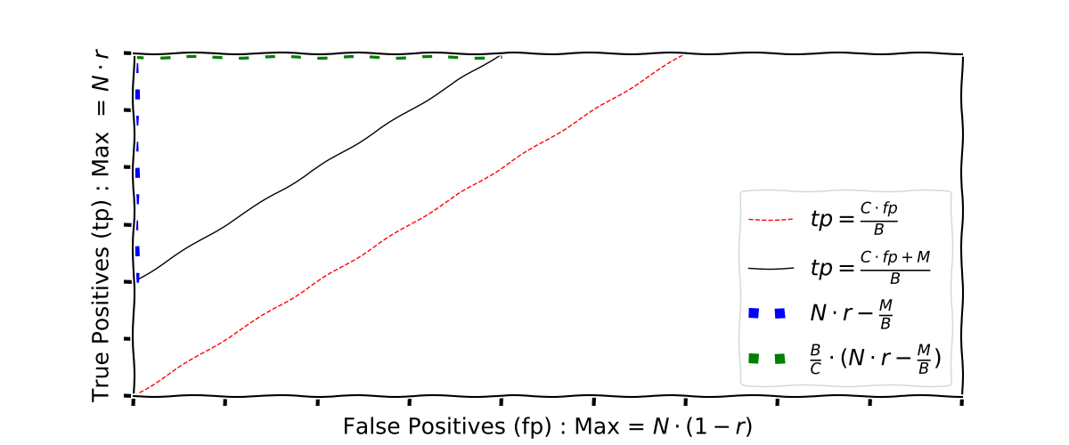
Figure 1: Schematic representation of potential model outputs depicting the boundary between viable and inviable models.

This geometric representation suggests an additional metric for the feasibility of any given project. Note, that the triangle in the upper left corner represents all possible model outputs that would satisfy the stated criteria. The dimensions of this triangle are shown in the legend by the lines of blue and green squares. We can calculate the area of this triangle and express it as a proportion of the total area of the rectangle. This will result in a metric which is the proportion of all potential model outputs that are economically viable. We can define an expression for this ratio as shown in Equation 8.

$$simplicity=\frac{\mathcal{B}}{2\cdot\mathcal{C}\cdot N^{2}\cdot r(1-r)}\cdot\left(N\cdot r-\frac{\mathcal{M}}{\mathcal{B}}\right)$$ (8)

This simplicity measure allows us to rank the difficulty of problems based purely on their business criteria. As this metric is to be calculated in a discrete space, and it must deal with edge cases in which the triangle is truncated, we refer the reader to the source code for its complete calculation.

Our efforts to estimate additional requirements in terms of standard machine learning metrics are hindered by the requirement to know either the number of true positives or false positives in the minimal viable model. To move beyond this limitation we will employ numerical techniques to estimate the bounds on the model performance.

3.4 ROC Simulation

The ROC plot provides us with a method of examinining the performance of a binary classification model in a manner that does not depend on a specific threshold. As shown in the example plot 2 it depicts a range of TPR and FPR values across all the different potential thresholds of the model. Additionally, the ROC plot permits the definition of a non-threshold specific metric to evaluate the overall discriminative power of the model (regardless of chosen threshold), the Area Under the Curve (AUC) [12].

We can generate synthetic ROC plots by exploiting their key properties.

1. They are necessarily monotonically increasing

2. They will necessarily pass through the points (0,0) and (1,1)

3. They remain above or on the diagonal between these points (unless the model is inversely calibrated)

We can simulate such curves by designing a parameterised function that satisfies these criteria. We have designed the function shown in equation 9 for this purpose. It is composed of two parts, both of which independantly satisfy the criteria.

$$y=\alpha\cdot(-(x-1)^{2\beta}+1)+(1-\alpha)\cdot x$$ (9)

In this function $\alpha$ is a weighting between zero and one that determines the mix between the two component functions. The first component function is an inverted even-powered polynomial function of x, offset so that its origin lies at coordinates (1,1). The second of function is just $x$ itself, which is the diagonal line. Both functions necessarily pass through the points $(0,0)$ and $(1,1)$, and their mixture determines the shape of the curve between these points.

Figure  2 shows some examples of simulated ROC plots with different values of the parameters $\alpha$ and $\beta$. Note, it is critical to restrict the space of these parameters such that the search space does not result in unrealistic ROC plots. The third plot in Figure  2 demonstrates that at extreme values the curve starts to represent a spline of two linear functions.

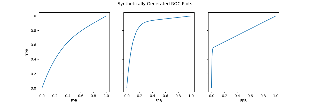
Figure 2: Examples of ROC plots generated through simulation.

By running simulations across a variety of values of $\alpha$ and $\beta$ we can generate multiple synthetic ROC plots. Each plot provides a set of hypothetical values for the true positive rate and false positive rate across a range of thresholds. If we combine these with the pre-defined characteristics of the problem we are solving (the number of cases, baseline rate, costs and benefits). Then we can identify which of these synthetic ROC plots would represent acceptable models. We can then rank them such that we search for the ROC curve with the minimum AUC that satisfies our ROI constraints.

Given a minimum viable AUC, we can then calculate estimates for the other metrics discussed above by taking the TPR and FPR values at the minimum viable threshold.

We have built a Python tool for running such simulations and released it as a Python package to the PyPI library (Available at $https://github.com/john-hawkins/MinViME$).

4.   Simulations

The MinViME tool allows us to explore the viable model landscape across a broad range of business criteria in order to understand what drives feasibility. In order to do so we need to represent the space of business problems in an informative and comprehensible way. We do so using the following three ratios.

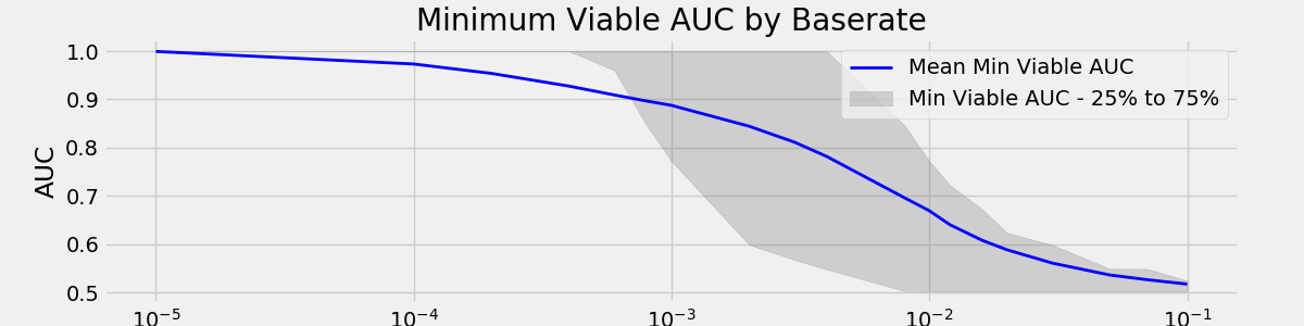
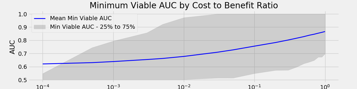
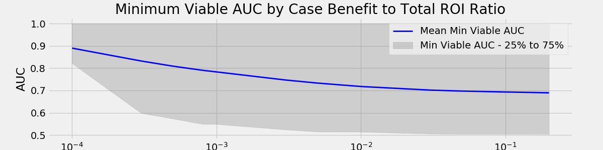
Figure 3: Relationship between the AUC of the minimum viable model and the criteria that determine the business problem. Note: We use a log scale on the X axis to demonstrate how the difficulty varies with each order of magnitude change in the nature of the problem.

1. Benefit to Total ROI. In other words how significant to the total required ROI is each additional true positive. We explore a range of values between zero and one.

2. Cost to Benefit. In other words how many false positives can we tolerate for every true positive case we identify. In principle this could take values greater than one, however this is almost never seen in practice so we explore a range of values between zero and one

3. Base Rate. The rate at which the event being predicted occurs in the population.

In addition, we use a static value of one million for the number of cases processed per unit of time This value is realistic for many problems and our experimentation with values an order of magnitude either side demonstrates little variation on the results presented below.

4.1 Results

In Figure 3 we see the mean minimum required AUC across each of the three dimensions. The gray bounds indicate the lower and upper quartiles. We see that problems get easier as either the base rate or the benefit to total ROI increases. The opposite occurs for the cost to benefit ratio as we would expect. The base rate plot demonstrates the most variability across the spectrum, with base rates between $10^{-3}$ and $10^{-2}$ demonstrating the largest variability. Above this range problems generally have less strenuous requirements and below it most problems require demanding model performance.

Elkan [5] observes that if we scale the entries in a cost matrix by a positive constant or if we add a constant to all entries, it will not affect the optimal decision. However, this is not true for determining the performance characterists of the minimum viable model. The interaction between the number of cases, the required ROI and the values in the cost matrix will mean that these changes can affect the characteristics of the minimum viable model.

When the benefit to total ROI ratio is very small we see that the model requirements are predominantly for an AUC above $0.8$. To further understand the relationship between the base rate and the cost to benefit ratio we plot the surface of required AUC for these values when the benefit to total ROI is $10^{-4}$.

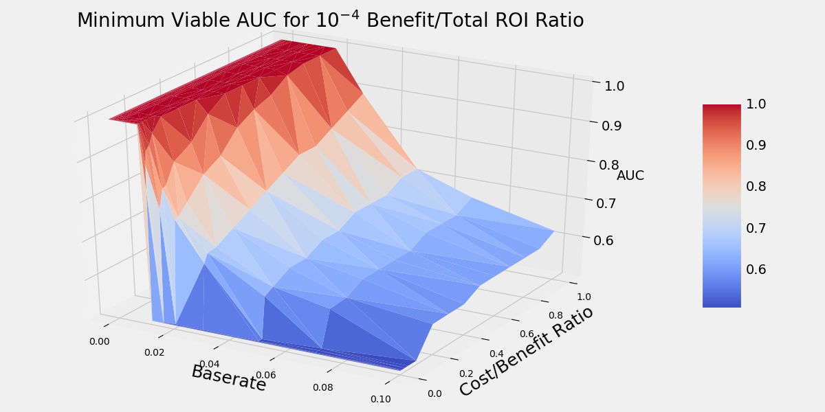
Figure 4: Surface of the AUC landscape for business problems in which each TP prediction returns $10^{-4}$ of the total required ROI

In Plot 4 we can see clearly that very low base rates can generate intractable problems that are likely to extremely difficult to solve. As the base rate increases we see a general weakening of the effect of the cost/benefit ratio. However, at very low cost/benefit ratios the impact of the base rate is almost entirely mitigated.

5.   Conclusion

We have discussed the problem of estimating the minimum viable performance characteristics of a machine learning model. The goal is to be able to do this before projects are undertaken so that we can make informed decisions about where our resources are most effectively deployed.

We investigated whether analytical lower bounds of standard machine learning performance metrics could be calculated from business criteria alone. We derived this for the model precision, and derived a novel simplicity metric which permits a priori comparisons of project complexity for binary classification systems.

We then demonstrated a numerical approach to estimating the minimum viable model performance through simulation of ROC plots. This in turn allows lower bound estimation of all other standard binary classification metrics. Using this method we explored the space of minimum viable models for a range of business problem characteristics. What we observe are some critical non-linear relationships between the base rate and the cost/benefit ratio that will determine whether a project is feasible or likely to be intractable.

© 2020 By AIRCC Publishing Corporation. This article is published under the Creative Commons Attribution(CC BY) license.

References

- [1] J. Johnson and T. Khoshgoftaar, “Medicare fraud detection using neural networks,” Journal of Big Data, vol. 63, no. 6, 2019. [Online]. Available: https://doi.org/10.1186/s40537-019-0225-0
- [2] C. Hennig and M. Kutlukaya, “Some thoughts about the design of loss functions,” REVSTAT - Statistical Journal Volume, vol. 5, pp. 19–39, 04 2007.
- [3] P. Domingos, “Metacost: A general method for making classifiers cost-sensitive,” Proceedings of the Fifth ACM SIGKDD Int’l. Conf. on Knowledge Discovery & Data Mining, pp. 155–164, 8 1999.
- [4] D. D. Margineantu, “On class-probability estimates and cost-sensitive evaluation of classifiers,” in In Workshop on Cost-Sensitive Learning at the Seventeenth International Conference on Machine Learning (WCSL at ICML2000, 2000.
- [5] C. Elkan, “The foundations of cost-sensitive learning,” Proceedings of the Seventeenth International Conference on Artificial Intelligence: 4-10 August 2001; Seattle, vol. 1, 05 2001.
- [6] Y. Tian and W. Zhang, “Thors: An efficient approach for making classifiers cost-sensitive,” IEEE Access, vol. 7, pp. 97 704–97 718, 2019.
- [7] H. Fatlawi, “Enhanced classification model for cervical cancer dataset based on cost sensitive classifier,” 08 2017.
- [8] N. Nikolaou, N. Edakunni, M. Kull, P. Flach, and G. Brown, “Cost-sensitive boosting algorithms: Do we really need them?” Machine Learning, vol. 104, 08 2016.
- [9] O. Ylijoki, “Guidelines for assessing the value of a predictive algorithm: a case study,” Journal of Marketing Analytics, vol. 6, 01 2018.
- [10] S. Raudys and A. Jain, “Small sample size effects in statistical pattern recognition: Recommendations for practitioners,” Pattern Analysis and Machine Intelligence, IEEE Transactions on, vol. 13, pp. 252–264, 04 1991.
- [11] I. E. Sanchez, “Optimal threshold estimation for binary classifiers using game theory,” ISCB Comm J, p. 2762, 2017. [Online]. Available: https://doi.org/10.12688/f1000research.10114.3
- [12] A. P. Bradley, “The use of the area under the roc curve in the evaluation of machine learning algorithms,” Pattern Recognition, vol. 30(7), pp. 1145–1159, 1997.