TenIPS: Inverse Propensity Sampling for Tensor Completion

Abstract

Tensors are widely used to represent multiway arrays of data. The recovery of missing entries in a tensor has been extensively studied, generally under the assumption that entries are missing completely at random (MCAR). However, in most practical settings, observations are missing not at random (MNAR): the probability that a given entry is observed (also called the propensity) may depend on other entries in the tensor or even on the value of the missing entry. In this paper, we study the problem of completing a partially observed tensor with MNAR observations, without prior information about the propensities. To complete the tensor, we assume that both the original tensor and the tensor of propensities have low multilinear rank. The algorithm first estimates the propensities using a convex relaxation and then predicts missing values using a higher-order SVD approach, reweighting the observed tensor by the inverse propensities. We provide finite-sample error bounds on the resulting complete tensor. Numerical experiments demonstrate the effectiveness of our approach.

1 Introduction

Tensor completion is gaining increasing popularity and is one of the major tensor-related research topics. The literature we survey here is by no means exhaustive. A straightforward method is to flatten a tensor along one of its dimensions to a matrix and then pick one of the extensively studied matrix completion algorithms [CT10, NW12, CZ13]. However, this method neglects the multiway structure along all other dimensions and does not make full use of the combinatorial relationships. Instead, it is common to assume that the tensor is low rank along each mode. Tensors differ from matrices in having many incompatible notions of rank and low rank decompositions, including CANDECOMP/PARAFAC (CP) [CC70, H⁺70], Tucker [Tuc66] and tensor-train [Ose11]. Each of the decompositions exploits a different definition of tensor rank, and can be used to recover tensors that are low rank in that sense, including CP [KS13, JO14, BM16, AW17, GPY18, LM20], Tucker [GRY11, MHWG14, XYZ17, YEG⁺18, Z⁺19, HN20] and tensor-train [WAA16, YZGC18]. In this paper, we assume the tensor has approximately low multilinear rank, corresponding to a tensor that can be approximated by a low rank Tucker decomposition.

Existing techniques used for tensor completion include subspace projection onto unfoldings [KS13], alternating minimization [JO14, LM20, WAA16], gradient descent [YZGC18] and expectation-maximization [YEG⁺18]; different surrogates for the rank penalty have been used, including convex surrogates like nuclear norm on unfoldings [THK10, GRY11, ATT18] or specific flattenings [MHWG14] and the maximum norm on factors [GPY18], and nonconvex surrogates such as the minimum number of rank-1 sign tensor components [GPY18]. We use a higher-order SVD (HOSVD) approach that does not require rank surrogates. The two methods closest to ours are HOSVD_w [HN20], which computes a weighted HOSVD by reweighting the tensor twice (before and after the HOSVD) by the inverse square root propensity, and the method in [XYZ17], which computes a HOSVD on a second-order estimator of a missing completely at random tensor, and we call it SO-HOSVD. We compare our method with HOSVD_w and SO-HOSVD theoretically in Section 5.2 and numerically in Section 6.1.

Most previous works on tensor completion have used the assumption that entries are missing completely at random (MCAR). The missing not at random (MNAR) setting is less studied, especially for tensors. A missingness pattern is MNAR when the observation probabilities (also called propensities) of different entries are not equal and may depend on the entry values themselves. In the matrix MNAR setting, a popular observation model is 1-bit observations [DPVDBW14]: each entry is observed with a probability that comes from applying a differentiable function $\sigma:\mathbb{R}\rightarrow[0,1]$ to the corresponding entry in a parameter matrix, which is assumed to be low rank. Two popular convex surrogates for the rank have been used to estimate the parameter matrix from an entrywise binary observation pattern using a regularized likelihood approach: nuclear norm [DPVDBW14, MC19, ATT18] and max-norm [CZ13, GPY18]. We show that we can achieve a small propensity estimation error by solving for a parameter tensor with low multilinear rank using a (roughly) square flattening. This approach outperforms simple slicing or flattening methods.

In this paper, we study the problem of provably completing a MNAR tensor with (approximately) low multilinear rank. We use a two-step procedure to first estimate the propensities in this tensor and then predict missing values by HOSVD on the inverse propensity reweighted tensor. We give the error bound on final estimation as Theorem 4.

This paper is organized as follows. Section 2 sets up our notations. Section 3 formally describes the problem we tackle in this paper. Section 4 gives an overview of our algorithms. Section 5 gives further clarification and finite sample error bounds for the algorithms. Section 6 shows numerical experiments.

2 Notations

Basics

We define $[N]=\{1,\ldots,N\}$ for a positive integer $N$. Given a set $S$, we denote its cardinality by $|S|$. $\subset$ denotes strict subset. We denote $f(n)=O(g(n))$ if there exists $C>0$ and $N$ such that $|f(n)|\leq Cg(n)$ for all $n\geq N$. The indicator function $\mathbf{1}(X)$ has value 1 if the condition $X$ is true, and 0 otherwise.

Matrices and tensors

We denote vector, matrix, and tensor variables respectively by lowercase letters ($x$), capital letters ($X$) and Euler script letters ($\mathscr{{X}}$). For a matrix $X\in\mathbb{R}^{m\times n}$, $\sigma_{1}(X)\geq\sigma_{2}(X)\geq\cdots\geq\sigma_{\min\{m,n\}}(X)$ denote its singular values, $\|X\|$ denotes its 2-norm, $\|X\|_{\star}$ denotes its nuclear norm, $\mathrm{tr}(X)$ denotes its trace, and with another matrix $Y\in\mathbb{R}^{m\times n}$, $\langle X,Y\rangle:=\mathrm{tr}(X^{\top}Y)$ denotes the matrix inner product. For a tensor $\mathscr{{X}}\in\mathbb{R}^{I_{1}\times I_{2}\times\cdots\times I_{N}}$, $\|\mathscr{{X}}\|_{\infty}$ denotes its entrywise maximum absolute value. The order of a tensor is the number of dimensions; matrices are order-two tensors. Each dimension is called a mode. To denote a part of matrix or tensor, we use a colon to denote the mode that is not fixed: given a matrix $A\in\mathbb{R}^{I\times J}$, $A_{i,:}$ and $A_{:,j}$ denote the $i$th row and $j$th column of $A$, respectively. A fiber is a one-dimensional section of a tensor $\mathscr{{X}}$, defined by fixing every index but one; for example, a fiber of the order-3 tensor $\mathscr{{X}}$ is $X_{:,j,k}$. A slice is an $(N-1)$-dimensional section of an order-$N$ tensor $\mathscr{{X}}$: a slice of the order-3 tensor $\mathscr{{X}}$ is $X_{:,:,k}$. The size of a mode is the number of slices along that mode: the $n$-th mode of $\mathscr{{X}}$ has size $I_{n}$. A tensor is cubical if every mode is the same size: $\mathscr{{X}}\in\mathbb{R}^{I\times I\times\cdots\times I}$. The mode-$n$ unfolding of $\mathscr{{X}}$, denoted as $\mathscr{{X}}^{(n)}$, is a matrix whose columns are the mode-$n$ fibers of $\mathscr{{X}}$. For example, given an order-3 tensor $\mathscr{{X}}\in\mathbb{R}^{I\times J\times K}$, $\mathscr{{X}}^{(1)}\in\mathbb{R}^{I\times(J\times K)}$.

Products

We denote the $n$-mode product of a tensor $\mathscr{{X}}\in\mathbb{R}^{I_{1}\times I_{2}\times\cdots\times I_{N}}$ with a matrix $U\in\mathbb{R}^{J\times I_{n}}$ by $\mathscr{{X}}\times_{n}U\in\mathbb{R}^{I_{1}\times\cdots\times I_{n-1}\times J\times I_{n+1}\times\cdots\times I_{N}}$; the $(i_{1},i_{2},\dots,i_{n-1},j,i_{n+1},\dots,i_{N})$-th entry is $\Sigma_{i_{n}=1}^{I_{n}}x_{i_{1}i_{2}\cdots i_{n-1}i_{n}i_{n+1}\cdots i_{N}}u_{ji_{n}}$. $\otimes$ denotes the Kronecker product. Given two tensors with the same shape, we use $\odot$ to denote their entrywise product.

Missingness

Given a partially observed order-$N$ tensor $\mathscr{{X}}\in\mathbb{R}^{I_{1}\times\cdots\times I_{N}}$, we denote its observation pattern by $\Upomega\in\{0,1\}^{I_{1}\times\cdots\times I_{N}}$: the mask tensor of $\mathscr{{X}}$. It is a binary tensor that denotes whether each entry of $\mathscr{{X}}$ is observed or not. $\Upomega$ has the same shape as $\mathscr{{X}}$, with entry value 1 if the corresponding entry of $\mathscr{{X}}$ is observed, and 0 otherwise. With an abuse of notation, we call $\Omega:=\{(i_{1},i_{2},\dots,i_{N})|\Upomega_{i_{1},i_{2},\dots,i_{N}}=1\}$ the mask set of $\mathscr{{X}}$. Given a tensor $\mathscr{{X}}\in\mathbb{R}^{I_{1}\times I_{2}\times\cdots\times I_{N}}$, we use $\mathscr{{E}}(i_{1},i_{2},\dots,i_{N})$ to denote a binary tensor with the same shape as $\mathscr{{X}}$, with value 1 at the $(i_{1},i_{2},\dots,i_{N})$-th entry and 0 elsewhere.

Square unfoldings

Extending the notation of [MHWG14], with a matrix $A\in\mathbb{R}^{I\times J}$ and integers $I^{\prime},J^{\prime}$ satisfying $IJ=I^{\prime}J^{\prime}$, $\texttt{reshape}(A,I^{\prime},J^{\prime})$ gives an $I^{\prime}\times J^{\prime}$ matrix $A^{\prime}$ with entries taken columnwise from $A$. Given a tensor $\mathscr{{X}}\in\mathbb{R}^{I_{1}\times I_{2}\times\cdots\times I_{N}}$, we can partition the indices of its $N$ modes into two sets, $S$ and $S^{C}=[N]\setminus S$, and permute the order of the $N$ modes by permutation $\pi_{S}=(S_{1},\ldots,S_{|S|},S^{C}_{1},\ldots,S^{C}_{N-|S|})$, so that the modes in set $S$ appear first, followed by modes in $S^{C}$:

$$\mathscr{{X}}_{i_{1}\cdots i_{N}}=\pi_{S}(\mathscr{{X}})_{i_{S_{1}}}\cdots i_{S_{|S|}}i_{S^{C}_{1}}\cdots i_{S^{C}_{N-|S|}}.$$

Denote the $S$-unfolding of $\mathscr{{X}}$ as

$$\mathscr{{X}}_{S}:=\texttt{reshape}(\pi_{S}(\mathscr{{X}})^{(1)},\prod_{n\in S}I_{n},\prod_{n\in S^{C}}I_{n}).$$

Our methods for tensor completion rely on methods for matrix completion that work best for square matrices. To make $\mathscr{{X}}_{S}$ as square as possible, $\Bigl{|}\prod_{n\in S}I_{n}-\prod_{n\in S^{C}}I_{n}\Bigr{|}$ should be as small as possible. Hence we define the square set of $\mathscr{{X}}$ as

$$S_{\square}=\underset{S\subset[N]}{\text{arg min}}\Bigl{|}\prod_{n\in S}I_{n}-\prod_{n\in S^{C}}I_{n}\Bigr{|},$$

the square unfolding of $\mathscr{{X}}$ as

$$\mathscr{{X}}_{\square}:=\texttt{reshape}(\pi_{S_{\square}}(\mathscr{{X}})^{(1)},\prod_{n\in S_{\square}}I_{n},\prod_{n\in S^{C}_{\square}}I_{n}),$$

and the square norm $\|\mathscr{{X}}\|_{\square}:=\|\mathscr{{X}}_{\square}\|_{\star}$ of $\mathscr{{X}}$.

Dimensions of unfoldings

For brevity, we denote $I_{S}:=\prod_{n\in S}I_{n}$, $I_{S^{C}}:=\prod_{n\in S^{C}}I_{n}$, $I_{\square}:=\prod_{n\in S_{\square}}I_{n}$, $I_{\square^{C}}:=\prod_{n\in S_{\square}^{C}}I_{n}$, $I_{(-n)}:=\prod_{m\in[N],m\neq n}I_{m}$. Thus $I_{[N]}=\prod_{n\in[N]}I_{n}=I_{S}\cdot I_{S^{C}}=I_{\square}\cdot I_{\square^{C}}=I_{n}\cdot I_{(-n)}$.

3 Problem setting

In this paper, we study the following problem: given a partially observed tensor $\mathscr{{B}}_{\mathrm{obs}}\in\mathbb{R}^{I_{1}\times\cdots\times I_{N}}$ with MNAR entries, how can we recover its missing values?

Throughout the paper, we denote the true order-$N$ tensor we want to complete as $\mathscr{{B}}\in\mathbb{R}^{I_{1}\times\cdots\times I_{N}}$. For each $n\in[N]$, we suppose $I_{n}\leq I_{(-n)}:=\prod_{m\in[N],m\neq n}I_{m}$ for cleanliness. We assume there exists a propensity tensor $\mathscr{{P}}\in\mathbb{R}^{I_{1}\times I_{2}\times\cdots I_{N}}$, such that $\mathscr{{B}}_{i_{1}i_{2}\cdots i_{N}}$ is observed with probability $\mathscr{{P}}_{i_{1}i_{2}\cdots i_{N}}$. We observe the entries without noise: with the observation pattern $\Upomega$, $\mathscr{{B}}_{\mathrm{obs}}=\mathscr{{B}}\odot\Upomega$.

A tensor $\mathscr{{B}}$ has multilinear rank $(r_{1}^{\mathrm{true}},r_{2}^{\mathrm{true}},\ldots,r_{N}^{\mathrm{true}})$ if $r_{n}^{\mathrm{true}}$ is the rank of $\mathscr{{B}}^{(n)}$. For any $n\in[N]$, $r_{n}^{\mathrm{true}}\leq I_{n}$. We can write the Tucker decomposition of the tensor $\mathscr{{B}}$ as $\mathscr{{B}}=\mathscr{{G}}^{\mathrm{true}}\times_{1}U_{1}^{\mathrm{true}}\times\cdots\times_{N}U_{N}^{\mathrm{true}}$, with core tensor $\mathscr{{G}}^{\mathrm{true}}\in\mathbb{R}^{r_{1}^{\mathrm{true}}\times\cdots\times r_{N}^{\mathrm{true}}}$ and column orthonormal factor matrices $U_{n}^{\mathrm{true}}\in\mathbb{R}^{I_{n}\times r_{n}^{\mathrm{true}}}$ for $n\in[N]$.

We seek a fixed-rank approximation of $\mathscr{{B}}$ by a tensor with multilinear rank $(r_{1},r_{2},\cdots,r_{N})$: we want to find a core tensor $\mathscr{{W}}\in\mathbb{R}^{r_{1}\times r_{2}\times\cdots\times r_{N}}$ and $N$ factor matrices $Q_{n}\in\mathbb{R}^{I_{n}\times r_{n}}$, $n\in[N]$ with orthonormal columns, such that $\mathscr{{B}}\approx\mathscr{{W}}\times_{1}Q_{1}\times_{2}\cdots\times_{N}Q_{N}$. We generally seek a low multilinear rank decomposition with $r_{n}<I_{n}$.

4 Methodology

Algorithm 1 ConvexPE: Convex Propensity Estimation

1 mask tensor $\Upomega\in\mathbb{R}^{I_{1}\times\cdots\times I_{N}}$, link function $\sigma$, thresholds $\tau$, $\gamma$

2 estimated propensity tensor $\widehat{\mathscr{{P}}}$

3 Compute $S_{\square}$, the square set of $\Upomega$.

4 Compute best completion $\widehat{\mathscr{{A}}}_{\square}=\underset{\Gamma\in\mathcal{S}_{\tau,\gamma}}{\text{argmax}}\sum_{i=1}^{I_{\square}}\sum_{j=1}^{I_{\square^{C}}}[(\Upomega_{\square})_{ij}\log\sigma(\Gamma_{ij})+(1-(\Upomega_{\square})_{ij})\log(1-\sigma(\Gamma_{ij}))]$, where $\mathcal{S}_{\tau,\gamma}=\big{\{}\Gamma\in\mathbb{R}^{I_{\square}\times I_{\square^{C}}}:\|\Gamma\|_{\star}\leq\tau\sqrt{I_{[N]}},\|\Gamma\|_{\infty}\leq\gamma\big{\}}$.

5 Estimate propensities $\widehat{\mathscr{{P}}}=\sigma(\widehat{\mathscr{{A}}})$.

6 return $\widehat{\mathscr{{P}}}$

Algorithm 2 NonconvexPE: Nonconvex Propensity Estimation

1 mask tensor $\Upomega\in\mathbb{R}^{I_{1}\times\cdots\times I_{N}}$, link function $\sigma$, step size $t$, initialization $\{\bar{\mathscr{{G}}}^{\mathscr{{A}}},\bar{U}_{1}^{\mathscr{{A}}},\ldots,\bar{U}_{N}^{\mathscr{{A}}}\}$ (or target rank $(r_{1},\ldots,r_{N})$ with a certain initialization rule)

2 estimated propensity tensor $\widehat{\mathscr{{P}}}$

3 Initialize core tensor and factor matrices $\mathscr{{G}}^{\mathscr{{A}}},U_{1}^{\mathscr{{A}}},\ldots,U_{N}^{\mathscr{{A}}}\leftarrow\bar{\mathscr{{G}}}^{\mathscr{{A}}},\bar{U}_{1}^{\mathscr{{A}}},\ldots,\bar{U}_{N}^{\mathscr{{A}}}$.

4 Define objective

$$f(\mathscr{{G}}^{\mathscr{{A}}},\{U_{n}^{\mathscr{{A}}}\}_{n\in[N]}):=\sum_{i_{1}\cdots i_{N}}-\Upomega_{i_{1}\cdots i_{N}}\log\sigma(\widehat{\mathscr{{A}}}_{i_{1}\cdots i_{N}})-(1-\Upomega_{i_{1}\cdots i_{N}})\log(1-\sigma(\widehat{\mathscr{{A}}}_{i_{1}\cdots i_{N}})),$$

$$\text{in which }\widehat{\mathscr{{A}}}=\mathscr{{G}}^{\mathscr{{A}}}\times_{1}U_{1}^{\mathscr{{A}}}\times_{2}\cdots\times_{N}U_{N}^{\mathscr{{A}}}.$$

5 do

6      Compute gradients with respect to core tensor and factor matrices $\left(\frac{\partial f}{\partial\mathscr{{G}}^{\mathscr{{A}}}},\frac{\partial f}{\partial U_{1}^{\mathscr{{A}}}},\ldots,\frac{\partial f}{\partial U_{N}^{\mathscr{{A}}}}\right)$.

7      Perform gradient descent update: $\mathscr{{G}}^{\mathscr{{A}}},U_{1}^{\mathscr{{A}}},\ldots,U_{N}^{\mathscr{{A}}}\leftarrow\left(\mathscr{{G}}^{\mathscr{{A}}}-t\frac{\partial f}{\partial\mathscr{{G}}^{\mathscr{{A}}}},U_{1}^{\mathscr{{A}}}-t\frac{\partial f}{\partial U_{1}^{\mathscr{{A}}}},\ldots,U_{N}^{\mathscr{{A}}}-t\frac{\partial f}{\partial U_{N}^{\mathscr{{A}}}}\right)$.

8 while not converged

9 Estimate propensities $\widehat{\mathscr{{P}}}=\sigma(\widehat{\mathscr{{A}}})$.

10 return $\widehat{\mathscr{{P}}}$

Algorithm 3 TenIPS: Tensor completion by Inverse Propensity Sampling

1 mask set $\Omega$, partially observed tensor $\mathscr{{B}}_{\text{obs}}\in\mathbb{R}^{I_{1}\times\cdots\times I_{N}}$, propensity tensor $\mathscr{{P}}\in\mathbb{R}^{I_{1}\times\cdots\times I_{N}}$, target rank $(r_{1},r_{2},\cdots,r_{N})$

2 estimated tensor $\widehat{\mathscr{{X}}}(\mathscr{{P}})$

3 $\bar{\mathscr{{X}}}(\mathscr{{P}})\leftarrow\sum_{(i_{1},i_{2},\ldots,i_{N})\in\Omega}\frac{1}{\mathscr{{P}}_{i_{1}i_{2}\cdots i_{N}}}\mathscr{{B}}_{\text{obs}}\odot\mathscr{{E}}(i_{1},i_{2},\dots,i_{N})$

4 for $n=1,2,\ldots,N$ do $\triangleright$ Recover factors

5      $Q_{n}(\mathscr{{P}})\leftarrow\text{left $r_{n}$ singular vectors of }\bar{\mathscr{{X}}}(\mathscr{{P}})^{(n)}$

6 $\mathscr{{W}}\leftarrow\bar{\mathscr{{X}}}(\mathscr{{P}})\times_{1}Q_{1}(\mathscr{{P}})^{\top}\times_{2}\cdots\times_{N}Q_{N}(\mathscr{{P}})^{\top}$ $\triangleright$ Recover core

7 $\widehat{\mathscr{{X}}}(\mathscr{{P}})\leftarrow\mathscr{{W}}(\mathscr{{P}})\times_{1}Q_{1}(\mathscr{{P}})\times_{2}\cdots\times_{N}Q_{N}(\mathscr{{P}})$

8 return $\widehat{\mathscr{{X}}}(\mathscr{{P}})$

Table 1: Propensity estimation algorithms.

	base algorithm	hyperparameters
ConvexPE (Algorithm 1)	proximal-proximal-gradient	$\tau$ and $\gamma$
NonconvexPE (Algorithm 2)	gradient descent	step size $t$ and target rank

Our algorithm proceeds in two steps. First, we estimate the propensities by ConvexPE (Algorithm 1) or NonconvexPE (Algorithm 2), with an overview in Table 1. Both of these algorithms use a Bernoulli maximum likelihood estimator for 1-bit matrix completion [DPVDBW14] to estimate the propensities from the mask tensor $\Upomega$, aiming to recover propensities that come from the low rank parameters. ConvexPE explicitly requires the propensities to be neither too large or too small. NonconvexPE does not require the associated tuning parameters, but empirically returns a good solution if the true propensity tensor $\mathscr{{P}}$ has this property. With the estimated propensity tensor $\widehat{\mathscr{{P}}}$, we estimate the data tensor $\mathscr{{B}}$ by TenIPS (Algorithm 3), a procedure that only requires a Tucker decomposition on the propensity-reweighted observations.

Our propensity estimation uses the observation model of 1-bit matrix completion. Each entry of $\mathscr{{P}}$ comes from applying a differentiable link function $\sigma:\mathbb{R}\rightarrow[0,1]$ to the corresponding entry of a parameter tensor $\mathscr{{A}}$, which we are trying to solve. An instance is the logistic function $\sigma(x)=1/(1+e^{-x})$. We assume $\mathscr{{A}}$ has low multilinear rank. In ConvexPE (Algorithm 1), $\mathscr{{A}}_{\square}$ is low-rank from Lemma 1. We also assume an upper bound on the nuclear norm of $\mathscr{{A}}_{\square}$, a convex surrogate for its low-rank property. ConvexPE can be implemented by the proximal-proximal-gradient method (PPG) [RY17] or the proximal alternating gradient descent. In Section 5, we will show that on a square tensor, the square unfolding achieves the smallest upper bound for propensity estimation among all possible unfoldings.

In practice, the square unfolding of a tensor is often a large matrix: $I^{N/2}$-by-$I^{N/2}$ for a cubical tensor with order $N$. Since each iteration of the PPG subroutine in ConvexPE requires the computation of a truncated SVD, this algorithm becomes too expensive in such case. Also, it does not make full use of the low multilinear rank property of $\mathscr{{A}}$. As a substitute, we propose NonconvexPE (Algorithm 2), which uses gradient descent (GD) on the core tensor $\mathscr{{G}}^{\mathscr{{A}}}$ and factor matrices $\{U_{n}^{\mathscr{{A}}}\}_{n\in[N]}$ to minimize the objective function $f(\mathscr{{G}}^{\mathscr{{A}}},\{U_{n}^{\mathscr{{A}}}\}_{n\in[N]})$ defined in Line 4. It achieves a feasible solution with similar quality as ConvexPE, and does not require the tuning of thresholds $\tau$ and $\gamma$. This can be attributed to the fact that the objective function $f$ is multi-convex with respect $(\mathscr{{G}}^{\mathscr{{A}}},U_{1}^{\mathscr{{A}}},\ldots,U_{N}^{\mathscr{{A}}})$. The gradient computation can be found in Appendix C.

TenIPS (Algorithm 3) completes the observed data tensor $\mathscr{{B}}_{\mathrm{obs}}$ by HOSVD on its entrywise inverse propensity reweighting $\bar{\mathscr{{X}}}(\mathscr{{P}})$, as defined in Line 2. For each $(i_{1},i_{2},\dots,i_{N})\in\Omega$, the corresponding term in $\bar{\mathscr{{X}}}(\mathscr{{P}})$ is an unbiased estimate for $\mathscr{{B}}\odot\mathscr{{E}}(i_{1},i_{2},\dots,i_{N})$:

$$\operatorname{\mathbb{E}}[\frac{1}{\mathscr{{P}}_{i_{1}i_{2}\cdots i_{N}}}\mathscr{{B}}_{\text{obs}}\odot\mathscr{{E}}(i_{1},i_{2},\dots,i_{N})] =\mathscr{{P}}_{i_{1}i_{2}\cdots i_{N}}\cdot\frac{1}{\mathscr{{P}}_{i_{1}i_{2}\cdots i_{N}}}\mathscr{{B}}_{\text{obs}}\odot\mathscr{{E}}(i_{1},i_{2},\dots,i_{N})$$

$$=\mathscr{{B}}\odot\mathscr{{E}}(i_{1},i_{2},\dots,i_{N}),$$

in which the second equality comes from noiseless observations. Thus $\bar{\mathscr{{X}}}(\mathscr{{P}})$ is an unbiased estimator for $\mathscr{{B}}$:

$$\operatorname{\mathbb{E}}\bar{\mathscr{{X}}}(\mathscr{{P}}) =\operatorname{\mathbb{E}}\Big{[}\sum_{(i_{1},i_{2},\dots,i_{N})\in\Omega}\frac{1}{\mathscr{{P}}_{i_{1}i_{2}\cdots i_{N}}}\mathscr{{B}}_{\text{obs}}\odot\mathscr{{E}}(i_{1},i_{2},\dots,i_{N})\Big{]}$$

$$=\sum_{i_{1}=1}^{I_{1}}\sum_{i_{2}=1}^{I_{2}}\cdots\sum_{i_{N}=1}^{I_{N}}\operatorname{\mathbb{E}}\Big{[}\frac{1}{\mathscr{{P}}_{i_{1}i_{2}\cdots i_{N}}}\mathscr{{B}}_{\text{obs}}\odot\mathscr{{E}}(i_{1},i_{2},\dots,i_{N})\Big{]}$$

$$=\sum_{i_{1}=1}^{I_{1}}\sum_{i_{2}=1}^{I_{2}}\cdots\sum_{i_{N}=1}^{I_{N}}\mathscr{{B}}\odot\mathscr{{E}}(i_{1},i_{2},\dots,i_{N})=\mathscr{{B}}.$$

The input propensity tensor can be either true ($\mathscr{{P}}$) or estimated ($\widehat{\mathscr{{P}}}$). With the estimated propensity $\widehat{\mathscr{{P}}}$, we get $\bar{\mathscr{{X}}}(\widehat{\mathscr{{P}}})$ instead of $\bar{\mathscr{{X}}}(\mathscr{{P}})$, $\widehat{\mathscr{{X}}}(\widehat{\mathscr{{P}}})$ instead of $\widehat{\mathscr{{X}}}(\mathscr{{P}})$; for brevity, we denote $\bar{\mathscr{{X}}}(\mathscr{{P}})$ and $\mathscr{{\widehat{X}}}(\mathscr{{P}})$ by $\bar{\mathscr{{X}}}$ and $\mathscr{{\widehat{X}}}$, respectively. We show the estimation error for $\mathscr{{B}}$ in Theorem 4.

5 Error analysis

To bound the relative estimation error $\|\widehat{\mathscr{{X}}}(\widehat{\mathscr{{P}}})-\mathscr{{B}}\|_{\mathrm{F}}/\|\mathscr{{B}}\|_{\mathrm{F}}$, we first bound the error in the propensity estimates in ConvexPE, and then consider how this error propagates into the error of our final tensor estimate in TenIPS. Theorem 3 shows the optimality of the square unfolding for propensity estimation; Theorem 4 presents a special case of our bound on the tensor completion error with estimated propensities, with the full version as Appendix A, Theorem 5. We defer their proofs to Appendix B.

5.1 Error in propensity estimates

We first show a corollary of [MHWG14, Lemma 6 (2) and Lemma 7] that bounds the rank of an unfolding.

Lemma 1.

Suppose $\mathscr{{X}}$ has Tucker decomposition $\mathscr{{X}}=\mathscr{{C}}\times_{1}U_{1}\times_{2}U_{2}\times_{3}\cdots\times_{N}U_{N}$, where $\mathscr{{C}}\in\mathbb{R}^{r_{1}^{\mathrm{true}}\times r_{2}^{\mathrm{true}}\times\cdots\times r_{N}^{\mathrm{true}}}$ and $U_{n}\in\mathbb{R}^{I_{n}\times r_{n}^{\mathrm{true}}}$ for $n\in[N]$. Given $S\subset[N]$, $\mathscr{{X}}_{S}=\underset{j\in S}{\otimes}U_{j}\cdot\mathscr{{C}}_{S}\cdot\Big{(}\underset{j\in[N]\backslash S}{\otimes}U_{j}\Big{)}^{\top}$, and thus $\mathrm{rank}(\mathscr{{X}}_{S})\leq\min\Bigl{\{}\prod_{n\in S}r_{n}^{\mathrm{true}},\,\prod_{n\in[N]\backslash S}r_{n}^{\mathrm{true}}\Big{\}}$.

Proof.

[MHWG14, Lemma 6 (2)] states that

$$\mathscr{{X}}_{[n]}=(U_{n}\otimes U_{n-1}\otimes\cdots\otimes U_{1})\,\mathscr{{C}}_{[n]}\,(U_{N}\otimes U_{N-1}\otimes\cdots\otimes U_{n+1})^{\top}$$ (1)

for $n\in[N]$. Thus Lemma 1 holds for $\mathscr{{X}}$ by applying Equation 1 to an entry-reordered tensor $\widetilde{\mathscr{{X}}}\in\mathbb{R}^{I_{n_{1}}\times I_{n_{2}}\times\cdots\times I_{n_{N}}}$, such that $S=\{n_{j}\}_{j\in[S]}$ and $\widetilde{\mathscr{{X}}}_{i_{n_{1}}i_{n_{2}}\cdots i_{n_{N}}}=\mathscr{{X}}_{i_{1}i_{2}\cdots i_{N}}$. The upper bound for $\mathrm{rank}(\mathscr{{X}}_{S})$ follows. ∎

As a corollary of [DPVDBW14, Lemma 1] and [MC19, Theorem 2], we have Lemma 2 for the Frobenius norm error of the propensity tensor estimate.

Lemma 2.

Assume that $\mathscr{{P}}=\sigma(\mathscr{{A}})$. Given a set $S\subset[N]$, together with the following assumptions:

• $\mathscr{{A}}_{S}$ has bounded nuclear norm: there exists a constant $\theta>0$ such that $\|\mathscr{{A}}_{S}\|_{\star}\leq\theta\sqrt{I_{[N]}}$.

• Entries of $\mathscr{{A}}$ have bounded absolute value: there exists a constant $\alpha>0$ such that $\|\mathscr{{A}}\|_{\infty}\leq\alpha$.

Suppose we run ConvexPE (Algorithm 1) with thresholds satisfying $\tau\geq\theta$ and $\gamma\geq\alpha$ to obtain an estimate $\mathscr{{\widehat{P}}}$ of $\mathscr{{P}}$. With $L_{\gamma}:=\sup_{x\in[-\gamma,\gamma]}\frac{|\sigma^{\prime}(x)|}{\sigma(x)(1-\sigma(x))}$, there exists a universal constant $C>0$ such that if $I_{S}+I_{S^{C}}\geq C$, with probability at least $1-\frac{C}{I_{S}+I_{S^{C}}}$, the estimation error

$$\frac{1}{I_{[N]}}\|\widehat{\mathscr{{P}}}-\mathscr{{P}}\|_{\mathrm{F}}^{2}\leq 4eL_{\gamma}\tau\Big{(}\frac{1}{\sqrt{I_{S}}}+\frac{1}{\sqrt{I_{S^{C}}}}\Big{)}.$$ (2)

In the simplest case, when $N$ is an even integer and $I_{1}=\ldots=I_{N}=I$, the right-hand side (RHS) of the estimation error in Equation 2 is in $O(I^{N/4})$.

Theorem 3 then shows that the square unfolding achieves the smallest upper bound for propensity estimation among all possible unfoldings sets $S$.

Theorem 3.

Instate the same conditions as Lemma 2, and further assume that there exists a constant $c>0$ such that $r_{n}^{\mathrm{true}}\leq cI_{n}$ for every $n\in[N]$. Then $S=S_{\square}$ gives the smallest upper bound (RHS of the result in Lemma 2) on the propensity estimation error $\|\widehat{\mathscr{{P}}}-\mathscr{{P}}\|_{\mathrm{F}}^{2}$ among all unfolding sets $S\subset[N]$.

Proof.

Denote $r_{S}^{\mathrm{true}}:=\prod_{n\in S}r_{n}^{\mathrm{true}}$ and $r_{S^{C}}^{\mathrm{true}}:=\prod_{n\in[N]\backslash S}r_{n}^{\mathrm{true}}$. We know from Lemma 1 of the main paper that for every unfolding of $\mathscr{{A}}$, $\mathrm{rank}({\mathscr{{A}}_{S}})\leq\min\Bigl{\{}r_{S}^{\mathrm{true}},\,r_{S^{C}}^{\mathrm{true}}\Big{\}}$. Since $\|\mathscr{{A}}_{S}\|_{\star}\leq\sqrt{\mathrm{rank}({\mathscr{{A}}_{S}})}\cdot\|\mathscr{{A}}\|_{\mathrm{F}}\leq\alpha\sqrt{\mathrm{rank}({\mathscr{{A}}_{S}})}\cdot I^{\frac{N}{2}}$, we need $\tau\geq\theta\geq\alpha\sqrt{\mathrm{rank}({\mathscr{{A}}_{S}})}$ for the conditions of Lemma 2 to hold. For simplicity, suppose $\tau=\alpha\sqrt{\mathrm{rank}({\mathscr{{A}}_{S}})}$, the smallest possible value for the exact recovery of $\mathscr{{A}}$.

Without loss of generality, suppose $|S|\leq\frac{N}{2}$. We have

$$\frac{1}{I_{[N]}}\|\widehat{\mathscr{{P}}}-\mathscr{{P}}\|_{\mathrm{F}}^{2} \leq 4eL_{\gamma}\tau\Big{(}\frac{1}{\sqrt{I_{S}}}+\frac{1}{\sqrt{I_{S^{C}}}}\Big{)}$$

$$=4eL_{\gamma}\alpha\cdot\sqrt{\mathrm{rank}({\mathscr{{A}}_{S}})}\Big{(}\frac{1}{\sqrt{I_{S}}}+\frac{1}{\sqrt{I_{S^{C}}}}\Big{)}$$

$$\leq 4eL_{\gamma}\alpha\Big{(}\sqrt{\frac{r_{S}^{\mathrm{true}}}{I_{S}}}+\sqrt{\frac{r_{S^{C}}^{\mathrm{true}}}{I_{S^{C}}}}\Big{)}$$

$$\leq 4eL_{\gamma}\alpha\Big{(}\sqrt{c^{|S|}}+\sqrt{c^{N-|S|}}\Big{)}.$$

The final expression is the smallest when $S=S_{\square}$. ∎

5.2 Error in tensor completion: special case

We present a special case of our bound on the recovery error for a cubical tensor with equal multilinear rank as Theorem 4. This bound is dominated by the error from the matrix Bernstein inequality [T⁺15] on each of the $N$ unfoldings, and asymptotically goes to 0 when the tensor size $I\rightarrow\infty$. Note that our full theorem applies to any tensor; we defer the formal statement to Appendix A, Theorem 5.

Theorem 4.

Consider an order-$N$ cubical tensor $\mathscr{{B}}$ with size $I_{1}=\cdots=I_{N}=I$ and multilinear rank $r_{1}^{\mathrm{true}}=\cdots=r_{N}^{\mathrm{true}}=r<I$, and two order-$N$ cubical tensors $\mathscr{{P}}$ and $\mathscr{{A}}$ with the same shape as $\mathscr{{B}}$. Each entry of $\mathscr{{B}}$ is observed with probability from the corresponding entry of $\mathscr{{P}}$. Assume $I\geq rN\log I$, and there exist constants $\psi,\alpha\in(0,\infty)$ such that $\|\mathscr{{A}}\|_{\infty}\leq\alpha$, $\|\mathscr{{B}}\|_{\infty}=\psi$. Further assume that for each $n\in[N]$, the condition number $\frac{\sigma_{1}(\mathscr{{B}}^{(n)})}{\sigma_{r}(\mathscr{{B}}^{(n)})}\leq\kappa$ is a constant independent of tensor sizes and dimensions. Then under the conditions of Lemma 2, with probability at least $1-I^{-1}$, the fixed multilinear rank $(r,r,\ldots,r)$ approximation $\widehat{\mathscr{{X}}}(\widehat{\mathscr{{P}}})$ computed from ConvexPE and TenIPS (Algorithms 1 and 3) with thresholds $\tau\geq\theta$ and $\gamma\geq\alpha$ satisfies

$$\frac{\|\widehat{\mathscr{{X}}}(\widehat{\mathscr{{P}}})-\mathscr{{B}}\|_{\mathrm{F}}}{\|\mathscr{{B}}\|_{\mathrm{F}}}\leq CN\sqrt{\frac{r\log I}{I}},$$ (3)

in which $C$ depends on $\kappa$.

Note how this bound compares with the bounds for similar algorithms. HOSVD_w has a relative error of $O(rN^{2}I^{-1/2}\log I)$ [HN20, Theorem 3.3] for noiseless recovery with known propensities, and SO-HOSVD achieves a better bound of $O(\sqrt{\frac{r\log I}{I^{N-1}}})$ [XYZ17, Theorem 3] but assumes that the tensor is MCAR. In contrast, our bound holds for the tensor MNAR setting and does not require known propensities. It is the first bound in this setting, to our knowledge.

We show a sketch of the proof for Theorem 4 to illustrate the main idea. This is the special case of the full proof in Appendix B.

Proof.

(sketch)

The propensity estimation error in Lemma 2, Equation 2 propagates to the error between $\bar{\mathscr{{X}}}(\widehat{\mathscr{{P}}})$ and $\bar{\mathscr{{X}}}(\mathscr{{P}})$:

$$\|\bar{\mathscr{{X}}}(\mathscr{{\widehat{P}}})-\bar{\mathscr{{X}}}\|_{\mathrm{F}}^{2}$$ (4)

$$=\sum_{({i_{1},i_{2},\dots,i_{N}})\in\Omega}\mathscr{{B}}_{i_{1}i_{2}\cdots i_{N}}^{2}(\frac{1}{\mathscr{{P}}_{i_{1}i_{2}\cdots i_{N}}}-\frac{1}{\mathscr{{\widehat{P}}}_{i_{1}i_{2}\cdots i_{N}}})^{2}$$

$$\leq\psi^{2}\sum_{({i_{1},i_{2},\dots,i_{N}})\in\Omega}\Big{(}\frac{\mathscr{{P}}_{i_{1}i_{2}\cdots i_{N}}-\mathscr{{\widehat{P}}}_{i_{1}i_{2}\cdots i_{N}}}{\mathscr{{P}}_{i_{1}i_{2}\cdots i_{N}}\mathscr{{\widehat{P}}}_{i_{1}i_{2}\cdots i_{N}}}\Big{)}^{2}$$

$$\leq\frac{\psi^{2}}{\sigma(-\gamma)^{2}\sigma(-\alpha)^{2}}\sum_{({i_{1},i_{2},\dots,i_{N}})\in\Omega}\Big{(}\mathscr{{P}}_{i_{1}i_{2}\cdots i_{N}}-\mathscr{{\widehat{P}}}_{i_{1}i_{2}\cdots i_{N}}\Big{)}^{2}$$

$$\leq\frac{4eL_{\gamma}\tau\psi^{2}}{\sigma(-\gamma)^{2}\sigma(-\alpha)^{2}}\Big{(}\frac{1}{\sqrt{I_{S}}}+\frac{1}{\sqrt{I_{S^{C}}}}\Big{)}I_{[N]}.$$

The second inequality comes from $\mathscr{{\widehat{P}}}_{i_{1}i_{2}\cdots i_{N}}\geq\sigma(-\gamma)$ and $\mathscr{{P}}_{i_{1}i_{2}\cdots i_{N}}\geq\sigma(-\alpha)$; the last inequality follows Lemma 2.

Then on each of the $N$ unfoldings, the error of $\bar{\mathscr{{X}}}^{(n)}(\widehat{\mathscr{{P}}})$ from $\mathscr{{B}}^{(n)}$

$$\|\bar{\mathscr{{X}}}^{(n)}(\mathscr{{\widehat{P}}})-\mathscr{{B}}^{(n)}\| \leq\|\bar{\mathscr{{X}}}^{(n)}(\mathscr{{\widehat{P}}})-\bar{\mathscr{{X}}}^{(n)}\|+\|\bar{\mathscr{{X}}}^{(n)}-\mathscr{{B}}^{(n)}\|$$ (5)

$$\leq\|\bar{\mathscr{{X}}}^{(n)}(\mathscr{{\widehat{P}}})-\bar{\mathscr{{X}}}^{(n)}\|_{\mathrm{F}}+\|\bar{\mathscr{{X}}}^{(n)}-\mathscr{{B}}^{(n)}\|,$$

in which the first term can be bounded by Equation 4, and the second term can be bounded by applying the matrix Bernstein inequality [T⁺15] to the sum of $[\frac{\mathbf{1}(\mathscr{{B}}_{i_{1}\cdots i_{N}}\text{ is observed})}{\mathscr{{P}}_{i_{1}\cdots i_{N}}}\mathscr{{B}}_{\text{obs}}-\mathscr{{B}}]\odot\mathscr{{E}}(i_{1},\dots,i_{N})$ over all entries.

The tensor $\bar{\mathscr{{X}}}(\mathscr{{\widehat{P}}})-\mathscr{{B}}$ is often full-rank; if we directly use $\sqrt{I}\cdot\|\bar{\mathscr{{X}}}^{(n)}(\mathscr{{\widehat{P}}})-\mathscr{{B}}^{(n)}\|$ to bound $\|\bar{\mathscr{{X}}}(\mathscr{{\widehat{P}}})-\mathscr{{B}}\|_{\mathrm{F}}$, the final error bound we get would be $O(N\sqrt{\log I})$, which increases with the increase of tensor size $I$. Instead, we use the information of low multilinear rank to form the estimator $\mathscr{{\widehat{X}}}(\mathscr{{\widehat{P}}})$. In TenIPS (Algorithm 3),

$$\mathscr{{\widehat{X}}}(\mathscr{{\widehat{P}}}) =[\bar{\mathscr{{X}}}(\mathscr{{\widehat{P}}})\times_{1}Q_{1}^{\top}\times_{2}\cdots\times_{N}Q_{N}^{\top}]\times_{1}Q_{1}\times_{2}\cdots\times_{N}Q_{N}$$

$$=\bar{\mathscr{{X}}}(\mathscr{{\widehat{P}}})\times_{1}Q_{1}Q_{1}^{\top}\times_{2}\cdots\times_{N}Q_{N}Q_{N}^{\top},$$

in which each $Q_{n}$ is the column space of $\bar{\mathscr{{X}}}^{(n)}(\mathscr{{\widehat{P}}})$. This projects each unfolding of $\bar{\mathscr{{X}}}(\mathscr{{\widehat{P}}})$ onto its truncated column space. By adding and subtracting $\mathscr{{B}}\times_{1}Q_{1}Q_{1}^{\top}\times_{2}\cdots\times_{N}Q_{N}Q_{N}^{\top}$, the projection of $\mathscr{{B}}$ onto the column space of $\bar{\mathscr{{X}}}(\mathscr{{\widehat{P}}})$ in each mode, we get the estimation error

$$\|\mathscr{{\widehat{X}}}(\mathscr{{\widehat{P}}})-\mathscr{{B}}\|_{\mathrm{F}}^{2}$$

$$=\|\bar{\mathscr{{X}}}(\mathscr{{\widehat{P}}})\times_{1}Q_{1}Q_{1}^{\top}\times_{2}\cdots\times_{N}Q_{N}Q_{N}^{\top}-\mathscr{{B}}\|_{\mathrm{F}}^{2}$$

$$=\|(\bar{\mathscr{{X}}}(\mathscr{{\widehat{P}}})-\mathscr{{B}})\times_{1}Q_{1}Q_{1}^{\top}\times_{2}\cdots\times_{N}Q_{N}Q_{N}^{\top}\|_{\mathrm{F}}^{2}$$

$$\quad+\|\mathscr{{B}}\times_{1}Q_{1}Q_{1}^{\top}\times_{2}\cdots\times_{N}Q_{N}Q_{N}^{\top}-\mathscr{{B}}\|_{\mathrm{F}}^{2}$$

$$\quad+2\langle(\bar{\mathscr{{X}}}(\mathscr{{\widehat{P}}})-\mathscr{{B}})\times_{1}Q_{1}Q_{1}^{\top}\times_{2}\cdots\times_{N}Q_{N}Q_{N}^{\top},\;\mathscr{{B}}\times_{1}Q_{1}Q_{1}^{\top}\times_{2}\cdots\times_{N}Q_{N}Q_{N}^{\top}-\mathscr{{B}}\rangle.$$

On the RHS, the third term is an inner product of two mutually orthogonal tensors and is thus 0. The first term is low multilinear rank, and thus can be bounded by the spectral norm of the unfoldings as

$$\|(\bar{\mathscr{{X}}}(\mathscr{{\widehat{P}}})-\mathscr{{B}})\times_{1}Q_{1}Q_{1}^{\top}\times_{2}\cdots\times_{N}Q_{N}Q_{N}^{\top}\|_{\mathrm{F}}^{2}$$

$$\leq\min_{n\in[N]}\Big{\{}\|Q_{n}Q_{n}^{\top}(\bar{\mathscr{{X}}}^{(n)}(\mathscr{{\widehat{P}}})-\mathscr{{B}}^{(n)})\|_{\mathrm{F}}^{2}\Big{\}}$$

$$\leq\min_{n\in[N]}\Big{\{}r\cdot\|\bar{\mathscr{{X}}}^{(n)}(\mathscr{{\widehat{P}}})-\mathscr{{B}}^{(n)}\|^{2}\Big{\}}.$$

The second term can be bounded by the sum of squares of residuals $\sum_{n\in[N]}\|\mathscr{{B}}\times_{n}(I-Q_{n}Q_{n}^{\top})\|_{\mathrm{F}}^{2}$. Each of the summand here is the perturbation error of $Q_{n}$ on the column space of $\mathscr{{B}}^{(n)}$, and thus can be bounded by the Davis-Kahan sin($\Theta$) Theorem [DK70, Wed72, YWS15]. ∎

6 Experiments

All the code is in the GitHub repository at https://github.com/udellgroup/TenIPS. We ran all experiments on a Linux machine with Intel^® Xeon^® E7-4850 v4 2.10GHz CPU and 1056GB memory, and used the logistic link function $\sigma(x)=1/(1+e^{-x})$ throughout the experiments.

We use both synthetic and semi-synthetic data for evaluation. We first compare the propensity estimation performance under square and rectangular (along a specific mode) unfoldings, and then compare the tensor recovery error under different approaches. For both propensity estimation and tensor completion, the relative error is defined as $\|\mathscr{{\widehat{T}}}-\mathscr{{T}}\|_{\mathrm{F}}/\|\mathscr{{T}}\|_{\mathrm{F}}$, in which $\mathscr{{\widehat{T}}}$ is the predicted tensor and $\mathscr{{T}}$ is the true tensor.

There are four algorithms similar to TenIPS for tensor completion in our experiments: SqUnfold, which performs SVD to seek the low-rank approximation of the square unfolding of the propensity-reweighted $\mathscr{{B}}_{\mathrm{obs}}$; RectUnfold, which applies SVD to the unfolding of the propensity-reweighted $\mathscr{{B}}_{\mathrm{obs}}$ along a specific mode; HOSVD_w [HN20] and SO-HOSVD [XYZ17]. The popular nuclear-norm-regularized least squares LstSq that seeks $\hat{B}=\underset{X}{\arg\min}\sum_{(i,j)\in\Omega}(B_{ij}-X_{ij})^{2}+\lambda\|X\|_{\star}$ on an unfolding of $\mathscr{{B}}_{\mathrm{obs}}$ takes much longer to finish in our experiments and is thus prohibitive in tensor completion practice, so we omit it from most of our results.

6.1 Synthetic data

We have the following observation models for synthetic tensors:

• MCAR. The propensity tensor $\mathscr{{P}}$ has all equal entries.

• MNAR with an approximatly low multilinear rank parameter tensor $\mathscr{{A}}$. One special case is that $\mathscr{{A}}$ is proportional to $\mathscr{{B}}$: a larger entry is more likely to be observed.

In the first experiment, we evaluate the performance of propensity estimation on synthetic tensors with approximately low multilinear rank. In each of the above observation models, we generate synthetic cubical tensors with equal size on each mode, and predict the propensity tensor by estimating the parameter tensor on either the square or rectangular unfolding.

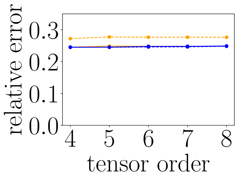
(a) Model A

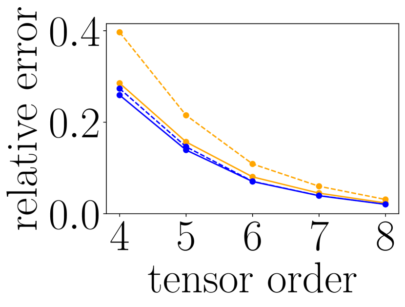
(b) Model B

[1pt]

Figure 1: Propensity estimation performance on different orders of tensors with size 8. The small size makes it possible to evaluate high-order tensors within a reasonable time. Figure 1(a) follows Model A with a $40\%$ observation ratio. Figure 1(b) follows Model B.

Figure 1 compares the propensity estimation error on tensors with different orders. For each $N$, with $I=8$ and $r=2$, we generate an order-$N$ parameter tensor $\mathscr{{A}}$ in the following way: We first generate $\mathscr{{A}}^{\natural}$ by Tucker decomposition $\mathscr{{G}}^{A}\times_{1}U^{A}_{1}\times\cdots\times_{N}U^{A}_{N}\in\mathbb{R}^{I\times\cdots\times I}$, in which $\mathscr{{G}}\in\mathbb{R}^{r\times\cdots\times r}$ has i.i.d. $\mathcal{N}(0,10^{2})$ entries, and each $U^{A}_{n}\in\mathbb{R}^{I\times r}$ has random orthonormal columns. Then we generate a noise-corrupted $\mathscr{{A}}$ by $\mathscr{{A}}^{\natural}+(\gamma\|\mathscr{{A}}^{\natural}\|_{\mathrm{F}}/I^{N/2})\upepsilon$, where the noise level $\gamma=0.1$ and the noise tensor $\upepsilon$ has i.i.d. $\mathcal{N}(0,1)$ entries. The “optimal” hyperparameter setting uses $\tau=\theta$ and $\gamma=\alpha$ in 1-bit matrix completion, and the “overestimated” setting, $\tau=2\theta$ and $\gamma=2\alpha$. We can see that:

1. The square unfolding is always better than the rectangular unfolding in achieving a smaller propensity estimation error.

2. The propensity estimation error on the square unfolding increases less when the optimization hyperparameters $\tau$ and $\gamma$ increase from their optima, $\theta$ and $\alpha$. This suggests that the square unfolding makes the constrained optimization problem more robust to the selection of optimization hyperparameters.

3. It is most important to use the square unfolding for higher-order tensors: the ratios of relative errors between overestimated and optimal increase from 1.3 to 1.4, while those on the square unfoldings stay at 1.1. This aligns with Theorem 3 that the square unfolding outperforms in the worst case.

In the second experiment, we complete tensors with MCAR entries. With $N=4$, $I=100$ and $r=5$, we generate an order-$N$ data tensor $\mathscr{{B}}\in\mathbb{R}^{I\times\cdots\times I}$ in the following way: We first generate $\mathscr{{B}}^{\natural}$ by $\mathscr{{G}}^{\mathrm{true}}\times_{1}U_{1}^{\mathrm{true}}\times_{2}\cdots\times_{N}U_{N}^{\mathrm{true}}$, in which $\mathscr{{G}}^{\mathrm{true}}\in\mathbb{R}^{r\times\cdots\times r}$ has i.i.d. $\mathcal{N}(0,100^{2})$ entries, and each $U_{n}^{\mathrm{true}}\in\mathbb{R}^{I\times r}$ has random orthonormal columns. Then we generate a noise-corrupted $\mathscr{{B}}$ by $\mathscr{{B}}^{\natural}+(\gamma\|\mathscr{{B}}^{\natural}\|_{\mathrm{F}}/I^{N/2})\upepsilon$, where the noise level $\gamma=0.1$ and the noise tensor $\upepsilon$ has i.i.d. $\mathcal{N}(0,1)$ entries.

TenIPS is competitive for MCAR. We compare the relative error of TenIPS with SqUnfold, RectUnfold and HOSVD_w at different observation ratios in Figure 2. We can see that TenIPS and HOSVD_w achieve the lowest recovery error on average, and the results of these two methods are nearly identical.

Figure 2: Error on MCAR tensors.

Figure 3: Propensity histogram in synthetic MNAR experiments.

Table 2: Completion performance on the order-4 MNAR synthetic cubical tensor with size 100. The “time” here is the time taken for the tensor completion step, with true or estimated propensities. $\widehat{\mathscr{{P}}}_{1}$ is from running the provable ConvexPE (Algorithm 1) at target rank 25 for 84 seconds, and has relative error 0.08 from the true tensor $\mathscr{{P}}$; $\widehat{\mathscr{{P}}}_{2}$ is from running the gradient-descent-based NonconvexPE (Algorithm 2) with i.i.d. Uniform$[-1,1]$ initialization and at step size $5\times 10^{-6}$ for 81 seconds, and has relative error 0.13. The bold number in each column indicates the best.

algorithm	time (s)	relative error from $\mathscr{{B}}$
		with $\mathscr{{P}}$	with $\widehat{\mathscr{{P}}}_{1}$	with $\widehat{\mathscr{{P}}}_{2}$
TenIPS	26	0.110	0.110	0.109
HOSVD_w	35	0.129	0.116	0.110
SqUnfold	29	0.141	0.138	0.139
RectUnfold	8	0.259	0.256	0.256
LstSq	>600	-	-	-
SO-HOSVD	>600	-	-	-

In the third experiment, we complete tensors with MNAR entries. We use the same $\mathscr{{B}}$ as the second experiment, and further generate an order-4 parameter tensor $\mathscr{{A}}\in\mathbb{R}^{100\times\cdots\times 100}$ in the same way as $\mathscr{{B}}$. $99.97\%$ of the propensities in $\mathscr{{P}}=\sigma(\mathscr{{A}})$ lie in the range of $[0.2,0.8]$, as shown in Figure 3. In Table 6.1, we see:

1. TenIPS outperforms for MNAR. It has the smallest error among methods that can finish within a reasonable time.

2. Tensor completion errors using estimated propensities are roughly equal to, and sometimes even smaller than those using true propensities despite a propensity estimation error.

3. On the sensitivity to hyperparameters: it is mentioned in the title of Table 6.1 that ConvexPE achieves a smaller accuracy within a similar time as NonconvexPE. However, this is because we set $\tau$ and $\gamma$ correctly: $\tau=\theta$ and $\gamma=\alpha$. In real cases, $\theta$ and $\alpha$ are unknown, and are hard to infer from surrogate metrics within the optimization process. The misestimates of $\theta$ and $\alpha$ may lead to large propensity estimation errors: As an example, ConvexPE with $\tau=100\theta$ and $\gamma=100\alpha$ never achieves a relative error smaller than $0.7$. Moreover, the relative error does not always decrease with more PPG iterations, despite the decrease of objective value. In every algorithm in Table 6.1, using these estimated propensities yields at least a relative error of $0.7$ for the estimation of data tensor $\mathscr{{B}}$. On the other hand, the initialization and step size in NonconvexPE can be tuned more easily by monitoring the value of function $f$ with the increase of number of iterations. More discussion can be found in Appendix D.

In the fourth experiment, we compare the above methods in both MCAR and MNAR settings when increasing target ranks.

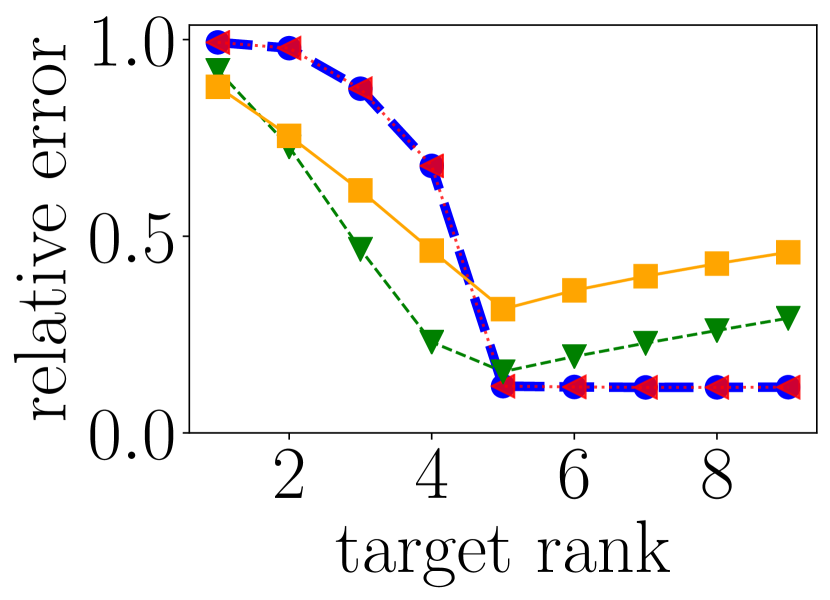
(a) Model A

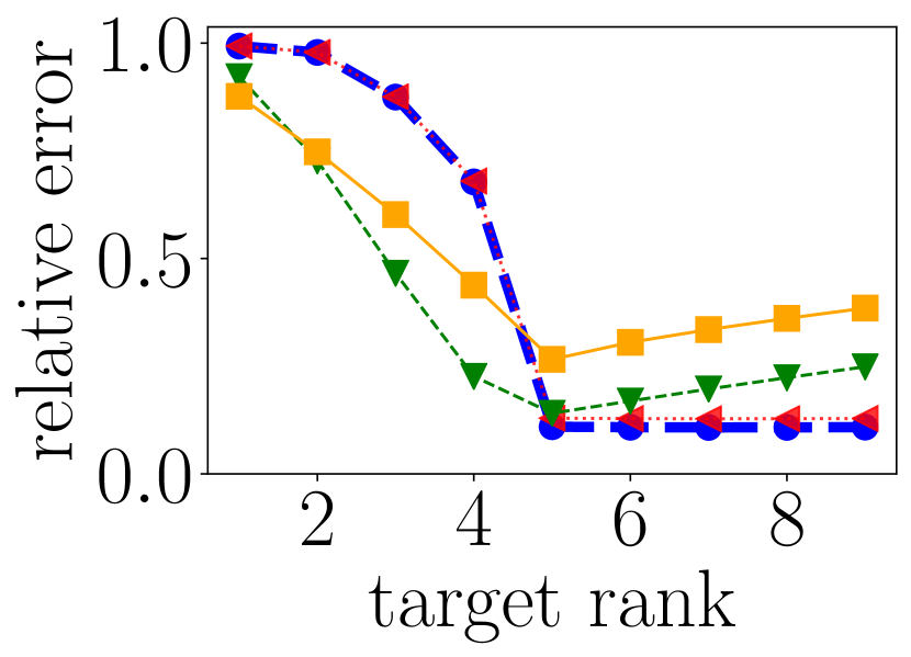
(b) Model B

Figure 4: Relative errors at different target ranks on the MNAR data from the third experiment. The true multilinear rank of the data tensor is 5 for each mode.

In Figure 4, we can see that both TenIPS and HOSVD_w are more stable at target ranks larger than the true rank, while RectUnfold and SqUnfold achieve smaller errors at smaller ranks. This shows that TenIPS and HOSVD_w are robust to large target ranks, which is the case when $r_{n}\geq r_{n}^{\mathrm{true}}$, for all $n\in[N]$.

6.2 Semi-synthetic data

We use the video from [MB18] and generate synthetic propensities. The video was taken by a camera mounted at a fixed position with a person walking by. We convert it to grayscale and discard the frames with severe vibration, which yields an order-3 data tensor $\mathscr{{B}}\in\mathbb{R}^{2200\times 1080\times 1920}$ that takes 102.0GB memory. To get an MNAR tensor $\mathscr{{B}}_{\mathrm{obs}}$, we generate the parameter tensor $\mathscr{{A}}$ by entrywise transformation $\mathscr{{A}}=(\mathscr{{B}}-128)/64$, which gives propensities in $[0.12,0.88]$ in $\mathscr{{P}}=\sigma(\mathscr{{A}})$. Finally we subsample $\mathscr{{B}}$ using propensities $\mathscr{{P}}$ to get $\mathscr{{B}}_{\mathrm{obs}}$.

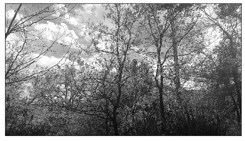
(a) original

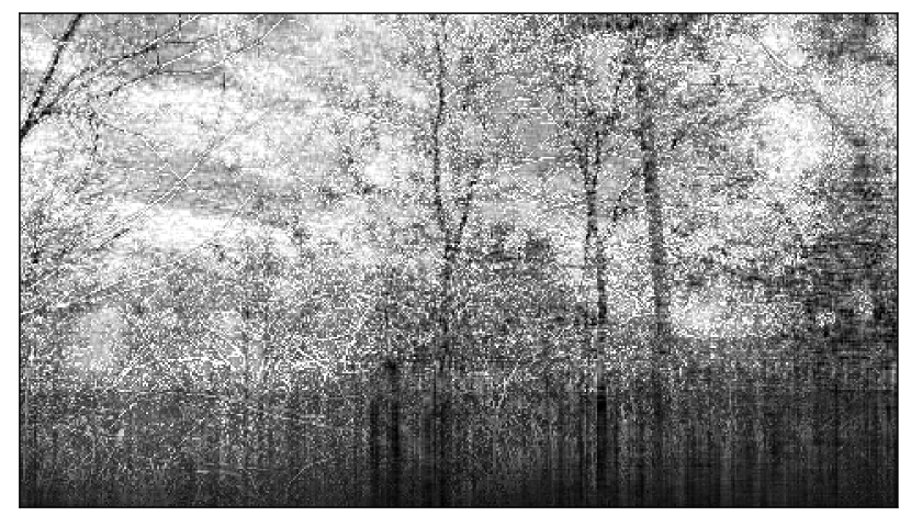
(b) TenIPS, assuming MCAR

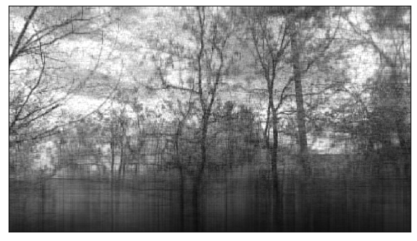
(c) TenIPS, assuming MNAR with true $\mathscr{{P}}$

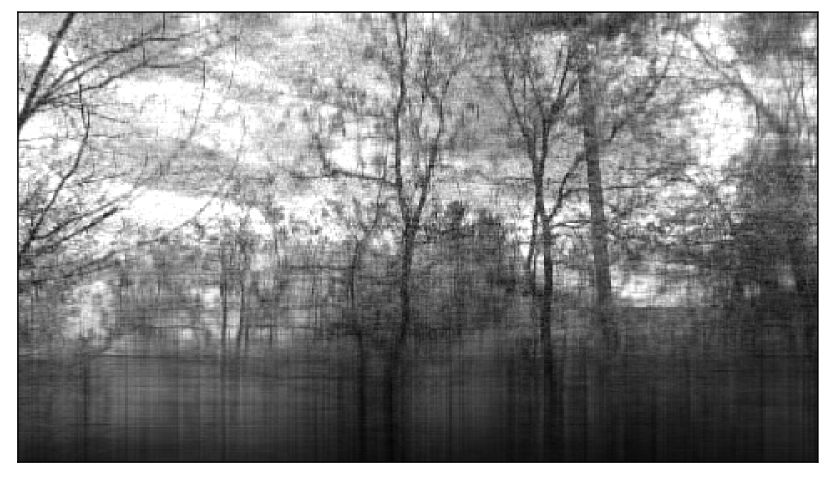
(d) TenIPS, assuming MNAR with estimated $\widehat{\mathscr{{P}}}$

Figure 5: Video recovery visualization on Frame 500 of the [MB18] video data. The missingness patterns in 5(b), 5(c) and 5(d) only refer to our assumption in tensor recovery; the partially observed data tensors we start from are the same and are MNAR.

We first compare the tensor completion performance of TenIPS with different sources of propensities. In Figure 5, we visualize the 500-th frame in three TenIPS experiments by fixed-rank approximation with target multilinear rank $(50,50,50)$: the original frame without missing pixels 5(a), the frame recovered under MCAR assumption (tensor recovery error 0.42) 5(b), the frame recovered by propensities under the MNAR assumption with the true propensity tensor $\mathscr{{P}}$ (tensor recovery error 0.28) 5(c), and the frame recovered by propensities under the MNAR assumption with the estimated propensity tensor $\widehat{\mathscr{{P}}}$ from ConvexPE (propensity estimation error 0.15, tensor recovery error 0.28) 5(d). We can see that:

1. With MNAR pixels, the image recovered from the naive MCAR assumption in Figure 5(b) is more noisy than that from MNAR in Figure 5(c) and 5(d), and misses more details.

2. There is no significant difference between the recovered video frames in 5(c) and 5(d), in terms of both the frame image itself and the tensor recovery error.

Table 3: Completion performance on the video task. The memory usages are those in Python 3. The bold number in each row indicates the best.

Setting	relative error (memory in GB)
	TenIPS	HOSVD_w	RectUnfold
I	0.28 (0.008)	0.44 (0.008)	0.14 (2.3)
II	0.20 (0.05)	0.31 (0.05)	0.25 (0.05)

We then compare TenIPS with HOSVD_w and RectUnfold on this video task; we omit SqUnfold and SO-HOSVD because SqUnfold and RectUnfold are equivalent on an order-3 tensor and SO-HOSVD cannot finish within a reasonable time. In Table 3 Setting I, TenIPS and HOSVD_w have target rank $(50,50,50)$, and RectUnfold has target rank $50$. We can see that RectUnfold has a smaller error in this setting but uses more than $250\times$ memory, because it does not seek low dimensional representations along the two dimensions of the video frame.

Another advantage of the tensor methods TenIPS and HOSVD_w compared to RectUnfold is that the target rank for different modes is not required to be the same. For example, if we limit memory usage to 0.05GB (Table 3, Setting II), TenIPS and HOSVD_w can afford a target rank $(5,500,500)$ and achieve smaller errors, while RectUnfold can only afford a target rank of $1$.

Also, with similar memory consumption in both settings, TenIPS achieves smaller errors than HOSVD_w.

7 Conclusion

This paper develops a provable two-step approach for MNAR tensor completion with unknown propensities. The square unfolding allows us to recover propensities with a smaller upper bound, and we then use HOSVD complete MNAR tensor with the estimated propensities. This method enjoys theoretical guarantee and fast running time in practice.

This paper is the first provable method for completing a general MNAR tensor. There are many avenues for improvement and extensions. For example, one could explore whether nonconvex matrix completion methods can be generalized to MNAR tensors, explore other observation models, and design provable algorithms that estimate the propensities even faster.

Acknowledgements

MU, CY, and LD gratefully acknowledge support from NSF Awards IIS-1943131 and CCF-1740822, the ONR Young Investigator Program, DARPA Award FA8750-17-2-0101, the Simons Institute, Canadian Institutes of Health Research, the Alfred P. Sloan Foundation, and Capital One. The authors thank Jicong Fan for helpful discussions, and thank several anonymous reviewers for useful comments.

Appendix A Error in tensor completion (ConvexPE and TenIPS): general case

We first state Theorem 5, the tensor completion error in the most general case. For brevity, we denote $\mathscr{{\widehat{X}}}(\mathscr{{P}})$ and $\bar{\mathscr{{X}}}(\mathscr{{P}})$ by $\mathscr{{\widehat{X}}}$ and $\bar{\mathscr{{X}}}$, respectively, in which $\mathscr{{P}}$ is the true propensity tensor.

Theorem 5.

Consider an order-$N$ tensor $\mathscr{{B}}\in\mathbb{R}^{I_{1}\times\cdots\times I_{N}}$, and two order-$N$ tensors $\mathscr{{P}}$ and $\mathscr{{A}}$ with the same shape as $\mathscr{{B}}$. Each entry $\mathscr{{B}}_{i_{1},\ldots,i_{N}}$ of $\mathscr{{B}}$ is observed with probability $\mathscr{{P}}_{i_{1},\ldots,i_{N}}$ from the corresponding entry of $\mathscr{{P}}$. Assume there exist constants $\psi,\alpha\in(0,\infty)$ such that $\|\mathscr{{A}}\|_{\infty}\leq\alpha$, $\|\mathscr{{B}}\|_{\infty}=\psi$. Denote the spikiness parameter $\alpha_{\mathrm{sp}}:=\psi\sqrt{I_{[N]}}/\|\mathscr{{B}}\|_{\mathrm{F}}$. Then under the conditions of Lemma 2, with probability at least $\displaystyle 1-\frac{C_{1}}{I_{\square}+I_{\square^{C}}}-\sum_{n=1}^{N}[I_{n}+I_{(-n)}]\exp\Big{[}-\frac{\epsilon^{2}\|\mathscr{{B}}\|_{\mathrm{F}}^{2}\sigma(-\alpha)/2}{I_{(-n)}\psi^{2}+\epsilon\psi\|\mathscr{{B}}\|_{\mathrm{F}}/3}\Big{]}$, in which $C_{1}>0$ is a universal constant, the fixed multilinear rank $(r_{1},r_{2},\cdots,r_{N})$ approximation $\widehat{\mathscr{{X}}}(\widehat{\mathscr{{P}}})$ computed from ConvexPE and TenIPS (Algorithms 1 and 3) with thresholds $\tau\geq\theta$ and $\gamma\geq\alpha$ satisfies

$$\frac{\|\widehat{\mathscr{{X}}}(\widehat{\mathscr{{P}}})-\mathscr{{B}}\|_{\mathrm{F}}^{2}}{\|\mathscr{{B}}\|_{\mathrm{F}}^{2}}\leq \min_{n\in[N]}\Bigg{\{}r_{n}\cdot\Big{[}\frac{\|\bar{\mathscr{{X}}}(\mathscr{{\widehat{P}}})-\bar{\mathscr{{X}}}\|_{\mathrm{F}}}{\|\mathscr{{B}}\|_{\mathrm{F}}}+\epsilon\Big{]}^{2}\Bigg{\}}$$ (6)

$$+\sum_{n=1}^{N}\frac{12r_{n}\sigma_{1}(\mathscr{{B}}^{(n)})^{2}}{\|\mathscr{{B}}\|_{\mathrm{F}}^{2}}\cdot\Bigg{\{}\frac{[2\sigma_{1}(\mathscr{{B}}^{(n)})+\|\bar{\mathscr{{X}}}(\mathscr{{\widehat{P}}})-\bar{\mathscr{{X}}}\|_{\mathrm{F}}+\epsilon\|\mathscr{{B}}\|_{\mathrm{F}}]^{2}}{[\sigma_{r_{n}}(\mathscr{{B}}^{(n)})+\sigma_{r_{n}+1}(\mathscr{{B}}^{(n)})]^{2}}\cdot\frac{[\|\bar{\mathscr{{X}}}(\mathscr{{\widehat{P}}})-\bar{\mathscr{{X}}}\|_{\mathrm{F}}+\epsilon\|\mathscr{{B}}\|_{\mathrm{F}}]^{2}}{[\sigma_{r_{n}}(\mathscr{{B}}^{(n)})-\sigma_{r_{n}+1}(\mathscr{{B}}^{(n)})]^{2}}\Bigg{\}}$$

$$+\frac{1}{\|\mathscr{{B}}\|_{\mathrm{F}}^{2}}\sum_{n=1}^{N}(\tau_{r_{n}}^{(n)})^{2},$$

in which:

1. $(\tau_{r_{n}}^{(n)})^{2}:=\sum_{i=r_{n}+1}^{I_{n}}\sigma_{i}^{2}(\mathscr{{B}}^{(n)})$ is the $r_{n}$-th tail energy for $\mathscr{{B}}^{(n)}$,

2. from Lemma 2, with $L_{\gamma}=\sup_{x\in[-\gamma,\gamma]}\frac{|\sigma^{\prime}(x)|}{\sigma(x)(1-\sigma(x))}$, and with probability at least $1-\frac{C_{1}}{I_{\square}+I_{\square^{C}}}$,

   $$\|\bar{\mathscr{{X}}}(\mathscr{{\widehat{P}}})-\bar{\mathscr{{X}}}\|_{\mathrm{F}}\leq\frac{\alpha_{\mathrm{sp}}\|\mathscr{{B}}\|_{\mathrm{F}}}{\sigma(-\gamma)\sigma(-\alpha)}\sqrt{4eL_{\gamma}\tau\Big{(}\frac{1}{\sqrt{I_{\square}}}+\frac{1}{\sqrt{I_{\square^{C}}}}\Big{)}}.$$ (7)

On the right-hand side of Equation 6, the first term comes from the error between $\bar{\mathscr{{X}}}(\mathscr{{P}})$ and $\mathscr{{B}}$ when projected onto the truncated column singular spaces in each mode $n\in[N]$; the second and third terms come from the projection error of $\mathscr{{B}}$ onto the above spaces.

Then, Theorem 4 is a corollary of the above Theorem 5 in the special case that the tensor is cubical and every unfolding has the same rank.

Appendix B Proof for Theorem 4 and 5

B.1 Proof for Theorem 5, the general case

We first show the proof for Theorem 5, the general case. This is the full version of the proof sketch in Section 5.2 of the main paper. We start with Lemma 6 on how the error in propensity estimates propagates to the error in the inverse propensity estimator $\bar{\mathscr{{X}}}(\widehat{\mathscr{{P}}})$, then bound the error between $\widehat{\mathscr{{X}}}(\widehat{\mathscr{{P}}})$ and $\mathscr{{B}}$.

Lemma 6.

Instate the conditions of Lemma 2 and further suppose $\|\mathscr{{B}}\|_{\infty}=\psi$. Then with probability at least $1-\frac{C_{1}}{I_{S}+I_{S^{C}}}$, in which $C_{1}>0$ is a universal constant,

$$\|\bar{\mathscr{{X}}}(\mathscr{{\widehat{P}}})-\bar{\mathscr{{X}}}\|_{\mathrm{F}}^{2}\leq\frac{4eL_{\gamma}\tau\psi^{2}}{\sigma(-\gamma)^{2}\sigma(-\alpha)^{2}}\Big{(}\frac{1}{\sqrt{I_{S}}}+\frac{1}{\sqrt{I_{S^{C}}}}\Big{)}I_{[N]}.$$ (8)

Proof.

Under the above conditions,

$$\|\bar{\mathscr{{X}}}(\mathscr{{\widehat{P}}})-\bar{\mathscr{{X}}}\|_{\mathrm{F}}^{2} =\sum_{({i_{1},i_{2},\dots,i_{N}})\in\Omega}\mathscr{{B}}_{i_{1}i_{2}\cdots i_{N}}^{2}(\frac{1}{\mathscr{{P}}_{i_{1}i_{2}\cdots i_{N}}}-\frac{1}{\mathscr{{\widehat{P}}}_{i_{1}i_{2}\cdots i_{N}}})^{2}$$

$$\leq\psi^{2}\sum_{({i_{1},i_{2},\dots,i_{N}})\in\Omega}\Big{(}\frac{\mathscr{{P}}_{i_{1}i_{2}\cdots i_{N}}-\mathscr{{\widehat{P}}}_{i_{1}i_{2}\cdots i_{N}}}{\mathscr{{P}}_{i_{1}i_{2}\cdots i_{N}}\mathscr{{\widehat{P}}}_{i_{1}i_{2}\cdots i_{N}}}\Big{)}^{2}$$

$$\leq\frac{\psi^{2}}{\sigma(-\gamma)^{2}\sigma(-\alpha)^{2}}\sum_{({i_{1},i_{2},\dots,i_{N}})\in\Omega}\Big{(}\mathscr{{P}}_{i_{1}i_{2}\cdots i_{N}}-\mathscr{{\widehat{P}}}_{i_{1}i_{2}\cdots i_{N}}\Big{)}^{2}$$

$$\leq\frac{4eL_{\gamma}\tau\psi^{2}}{\sigma(-\gamma)^{2}\sigma(-\alpha)^{2}}\Big{(}\frac{1}{\sqrt{I_{S}}}+\frac{1}{\sqrt{I_{S^{C}}}}\Big{)}I_{[N]}.$$

The second inequality comes from $\mathscr{{\widehat{P}}}_{i_{1}i_{2}\cdots i_{N}}\geq\sigma(-\gamma)$ and $\mathscr{{P}}_{i_{1}i_{2}\cdots i_{N}}\geq\sigma(-\alpha)$; the last inequality follows Lemma 2. ∎

We then state two lemmas that we will apply to tensor unfoldings. Lemma 7 is the matrix Bernstein inequality. Lemma 8 is a variant of the Davis-Kahan sin($\Theta$) Theorem [DK70].

Lemma 7 (Matrix Bernstein for real matrices [T⁺15, Theorem 1.6.2]).

Let $S_{1},\ldots,S_{k}$ be independent, centered random matrices with common dimension $m\times n$, and assume that each one is uniformly bounded

$$\operatorname{\mathbb{E}}S_{i}=0\quad\text{and}\quad\|S_{i}\|\leq L\quad\text{for each $i=1,\ldots,k$.}$$

Introduce the sum

$$Z=\sum_{i=1}^{k}S_{i},$$

and let $v(Z)$ denote the matrix variance statistic of the sum:

$$v(Z) =\max\big{\{}\|\smash{\operatorname{\mathbb{E}}(ZZ^{\top})}\|,\ \|\smash{\operatorname{\mathbb{E}}(Z^{\top}Z)}\|\big{\}}$$

$$=\max\left\{\|\sum_{i=1}^{k}\operatorname{\mathbb{E}}\big{(}S_{i}S_{i}^{\top}\big{)}\|,\ \|\sum_{i=1}^{k}\operatorname{\mathbb{E}}\big{(}S_{i}^{\top}S_{i}\big{)}\|\right\}.$$

Then

$$\mathbb{P}\left\{\|Z\|\geq t\right\}\leq(m+n)\cdot\exp\left(\frac{-t^{2}/2}{v(Z)+Lt/3}\right)\quad\text{for all $t\geq 0$.}$$

Lemma 8 (Variant of the Davis-Kahan sin($\Theta$) Theorem [Wed72], [YWS15, Theorem 4]).

Let $A,\smash{\widehat{A}}\in\mathbb{R}^{p\times q}$ have singular values $\sigma_{1}\geq\ldots\geq\sigma_{\min(p,q)}$ and $\widehat{\sigma}_{1}\geq\ldots\geq\widehat{\sigma}_{\min(p,q)}$ respectively, and have singular vectors $\{u_{i}\}_{i=1}^{n}$, $\{v_{i}\}_{i=1}^{n}$ and $\{\smash{\widehat{u}}_{i}\}_{i=1}^{n}$, $\{\smash{\widehat{v}}_{i}\}_{i=1}^{n}$, respectively. Let $V=(v_{1},\cdots,v_{r})\in\mathbb{R}^{n\times r}$, $\smash{\widehat{V}}=(\smash{\widehat{v}}_{1},\cdots,\smash{\widehat{v}}_{r})\in\mathbb{R}^{n\times r}$, $V_{\perp}=(v_{r+1},\cdots,v_{n})\in\mathbb{R}^{n\times(n-r)}$ and $\smash{\widehat{V}}_{\perp}=(\smash{\widehat{v}}_{r+1},\cdots,\smash{\widehat{v}}_{n})\in\mathbb{R}^{n\times(n-r)}$. Assume that $\sigma_{r}^{2}-\sigma_{r+1}^{2}>0$, then

$$\|\smash{\widehat{V}}_{\perp}^{\top}V\|_{\mathrm{F}}=\|V_{\perp}^{\top}\smash{\widehat{V}}\|_{\mathrm{F}}=\|\smash{\widehat{V}}\smash{\widehat{V}}^{\top}-VV^{\top}\|_{\mathrm{F}}\leq\frac{2(2\sigma_{1}+\|\smash{\widehat{A}}-A\|)\min(r^{1/2}\|\smash{\widehat{A}}-A\|,\|\smash{\widehat{A}}-A\|_{\mathrm{F}})}{\sigma_{r}^{2}-\sigma_{r+1}^{2}}.$$

Identical bounds also hold if $V$ and $\smash{\widehat{V}}$ are replaced with the matrices of left singular vectors $U$ and $\smash{\widehat{U}}$, where $U=(u_{r},u_{r+1},\ldots,u_{s})\in\mathbb{R}^{p\times d}$ and $\smash{\widehat{U}}=(\smash{\widehat{u}}_{r},\smash{\widehat{u}}_{r+1},\ldots,\smash{\widehat{u}}_{s})\in\mathbb{R}^{p\times d}$ have orthonormal columns satisfying $A^{\top}u_{j}=\sigma_{j}v_{j}$ and $\smash{\widehat{A}}^{\top}\hat{u}_{j}=\widehat{\sigma}_{j}\smash{\widehat{v}}_{j}$ for $j=r,r+1,\ldots,s$.

Upper bound on $\|\bar{\mathscr{{X}}}^{(n)}(\mathscr{{\widehat{P}}})-\mathscr{{B}}^{(n)}\|$:

We decompose it into the error between $\bar{\mathscr{{X}}}^{(n)}(\mathscr{{\widehat{P}}})$ and $\bar{\mathscr{{X}}}^{(n)}(\mathscr{{P}})$, and the error between $\bar{\mathscr{{X}}}^{(n)}(\mathscr{{P}})$ and $\mathscr{{B}}$, and independently bound these two terms:

$$\|\bar{\mathscr{{X}}}^{(n)}(\mathscr{{\widehat{P}}})-\mathscr{{B}}^{(n)}\| \leq\|\bar{\mathscr{{X}}}^{(n)}(\mathscr{{\widehat{P}}})-\bar{\mathscr{{X}}}^{(n)}\|+\|\bar{\mathscr{{X}}}^{(n)}-\mathscr{{B}}^{(n)}\|$$ (9)

$$\leq\|\bar{\mathscr{{X}}}^{(n)}(\mathscr{{\widehat{P}}})-\bar{\mathscr{{X}}}^{(n)}\|_{\mathrm{F}}+\|\bar{\mathscr{{X}}}^{(n)}-\mathscr{{B}}^{(n)}\|.$$

The first RHS term is bounded by Lemma 6, the error given by propensity estimation. Note that we can get a tighter bound if we can directly bound $\|\bar{\mathscr{{X}}}^{(n)}(\mathscr{{\widehat{P}}})-\bar{\mathscr{{X}}}^{(n)}\|$. The second RHS term can be bounded by Lemma 7, the matrix Bernstein inequality, as below.

For each $(i_{1},\dots,i_{N})$, define the random variable

$$\mathscr{{S}}_{i_{1}i_{2}\cdots i_{N}}:=\left\{\begin{aligned} &\Big{(}\frac{1}{\mathscr{{P}}_{i_{1}i_{2}\cdots i_{N}}}-1\Big{)}\mathscr{{B}}\odot\mathscr{{E}}(i_{1},i_{2},\dots,i_{N}),\quad&&\text{with probability $\mathscr{{P}}_{i_{1}i_{2}\cdots i_{N}}$}\\ &-\mathscr{{B}}\odot\mathscr{{E}}(i_{1},i_{2},\dots,i_{N}),\quad&&\text{with probability $1-\mathscr{{P}}_{i_{1}i_{2}\cdots i_{N}}$.}\end{aligned}\right.$$

With the assumptions in Theorem 5, $\operatorname{\mathbb{E}}\mathscr{{S}}_{i_{1}i_{2}\cdots i_{N}}=0$ and $\|\mathscr{{S}}_{i_{1}i_{2}\cdots i_{N}}^{(n)}\|\leq\frac{\psi}{\sigma(-\alpha)}$. Also, the per-mode second moment is bounded as

$$v_{n}(\mathscr{{X}}) =\max\{\|\sum_{i_{1}=1}^{I_{1}}\sum_{i_{2}=1}^{I_{2}}\cdots\sum_{i_{n}=1}^{I_{n}}\operatorname{\mathbb{E}}[\mathscr{{S}}_{i_{1}i_{2}\cdots i_{N}}^{(n)}(\mathscr{{S}}_{i_{1}i_{2}\cdots i_{N}}^{(n)})^{\top}]\|,\|\sum_{i_{1}=1}^{I_{1}}\sum_{i_{2}=1}^{I_{2}}\cdots\sum_{i_{n}=1}^{I_{n}}\operatorname{\mathbb{E}}[(\mathscr{{S}}_{i_{1}i_{2}\cdots i_{N}}^{(n)})^{\top}\mathscr{{S}}_{i_{1}i_{2}\cdots i_{N}}^{(n)}]\|\}$$

$$\leq\frac{\psi^{2}\cdot I_{(-n)}}{\sigma(-\alpha)}.$$

With probability at least $1-[I_{n}+I_{(-n)}]\exp\Big{[}-\frac{\epsilon^{2}\|\mathscr{{B}}\|_{\mathrm{F}}^{2}\sigma(-\alpha)/2}{I_{(-n)}\psi^{2}+\epsilon\psi\|\mathscr{{B}}\|_{\mathrm{F}}/3}\Big{]}$, the sum of random variables is bounded as $\displaystyle\|\sum_{i_{1}=1}^{I_{1}}\sum_{i_{2}=1}^{I_{2}}\cdots\sum_{i_{N}=1}^{I_{N}}\mathscr{{S}}_{i_{1}i_{2}\cdots i_{N}}\|\leq\epsilon\|\mathscr{{B}}\|_{\mathrm{F}}$. Notice the difference between the propensity-reweighted observed tensor $\bar{\mathscr{{X}}}(\mathscr{{P}})$ and the true tensor $\mathscr{{B}}$

$$\bar{\mathscr{{X}}}(\mathscr{{P}})-\mathscr{{B}} =\sum_{(i_{1},i_{2},\dots,i_{N})\in\Omega}\frac{1}{\mathscr{{P}}_{i_{1}i_{2}\cdots i_{N}}}\mathscr{{B}}_{\text{obs}}\odot\mathscr{{E}}(i_{1},i_{2},\dots,i_{N})-\mathscr{{B}}$$

$$=\sum_{(i_{1},i_{2},\dots,i_{N})\in\Omega}\Big{(}\frac{1}{\mathscr{{P}}_{i_{1}i_{2}\cdots i_{N}}}-1\Big{)}\mathscr{{B}}\odot\mathscr{{E}}(i_{1},i_{2},\dots,i_{N})-\sum_{(i_{1},i_{2},\dots,i_{N})\notin\Omega}\mathscr{{B}}\odot\mathscr{{E}}(i_{1},i_{2},\dots,i_{N})$$

is an instance of $\displaystyle\sum_{i_{1}=1}^{I_{1}}\sum_{i_{2}=1}^{I_{2}}\cdots\sum_{i_{N}=1}^{I_{N}}\mathscr{{S}}_{i_{1}i_{2}\cdots i_{N}}$ over the randomness of entry-wise observation, hence we can use the matrix Bernstein inequality (Lemma 7) to bound $\|\bar{\mathscr{{X}}}(\mathscr{{P}})-\mathscr{{B}}\|$. Together with Equations 8 and 9, we get the upper bound on $\|\bar{\mathscr{{X}}}^{(n)}(\mathscr{{\widehat{P}}})-\mathscr{{B}}^{(n)}\|$.

How $\|\bar{\mathscr{{X}}}^{(n)}(\mathscr{{\widehat{P}}})-\mathscr{{B}}^{(n)}\|$ propagates into the final error in TenIPS (Algorithm 3):

In TenIPS,

$$\mathscr{{\widehat{X}}}(\mathscr{{\widehat{P}}})=\underbrace{\left[\bar{\mathscr{{X}}}(\mathscr{{\widehat{P}}})\times Q_{1}^{\top}\times_{2}\cdots\times_{N}Q_{N}^{\top}\right]}_{\mathscr{{W}}(\mathscr{{\widehat{P}}})}\times_{1}Q_{1}\times_{2}\cdots\times_{N}Q_{N}=\bar{\mathscr{{X}}}(\mathscr{{\widehat{P}}})\times_{1}Q_{1}Q_{1}^{\top}\times_{2}\cdots\times_{N}Q_{N}Q_{N}^{\top}.$$

This projects each unfolding of $\bar{\mathscr{{X}}}(\mathscr{{\widehat{P}}})$ onto the space of its top left singular vectors. Thus by adding and subtracting $\mathscr{{B}}\times_{1}Q_{1}Q_{1}^{\top}\times_{2}\cdots\times_{N}Q_{N}Q_{N}^{\top}$ within the Frobenius norm, we decompose the error as

$$\|\mathscr{{\widehat{X}}}(\mathscr{{\widehat{P}}})-\mathscr{{B}}\|_{\mathrm{F}}^{2} =\|\bar{\mathscr{{X}}}(\mathscr{{\widehat{P}}})\times_{1}Q_{1}Q_{1}^{\top}\times_{2}\cdots\times_{N}Q_{N}Q_{N}^{\top}-\mathscr{{B}}\|_{\mathrm{F}}^{2}$$

$$=\|\bar{\mathscr{{X}}}(\mathscr{{\widehat{P}}})\times_{1}Q_{1}Q_{1}^{\top}\times_{2}\cdots\times_{N}Q_{N}Q_{N}^{\top}-\mathscr{{B}}\times_{1}Q_{1}Q_{1}^{\top}\times_{2}\cdots\times_{N}Q_{N}Q_{N}^{\top}$$

$$\quad+\mathscr{{B}}\times_{1}Q_{1}Q_{1}^{\top}\times_{2}\cdots\times_{N}Q_{N}Q_{N}^{\top}-\mathscr{{B}}\|_{\mathrm{F}}^{2}$$

$$=\underbrace{\|(\bar{\mathscr{{X}}}(\mathscr{{\widehat{P}}})-\mathscr{{B}})\times_{1}Q_{1}Q_{1}^{\top}\times_{2}\cdots\times_{N}Q_{N}Q_{N}^{\top}\|_{\mathrm{F}}^{2}}_{①}$$

$$+\underbrace{\|\mathscr{{B}}\times_{1}Q_{1}Q_{1}^{\top}\times_{2}\cdots\times_{N}Q_{N}Q_{N}^{\top}-\mathscr{{B}}\|_{\mathrm{F}}^{2}}_{②}$$

$$+\underbrace{2\langle(\bar{\mathscr{{X}}}(\mathscr{{\widehat{P}}})-\mathscr{{B}})\times_{1}Q_{1}Q_{1}^{\top}\times_{2}\cdots\times_{N}Q_{N}Q_{N}^{\top},\mathscr{{B}}\times_{1}Q_{1}Q_{1}^{\top}\times_{2}\cdots\times_{N}Q_{N}Q_{N}^{\top}-\mathscr{{B}}\rangle}_{③}.$$

First, we show that the cross term $③$ is zero, since it is the product of two terms in mutually orthogonal subspaces. For each $n\in[N]$,

$$[(\bar{\mathscr{{X}}}(\mathscr{{\widehat{P}}})-\mathscr{{B}})\times_{1}Q_{1}Q_{1}^{\top}\times_{2}\cdots\times_{N}Q_{N}Q_{N}^{\top}]^{(n)}=Q_{n}\mathscr{{C}}_{n}^{(n)},$$

where $\mathscr{{C}}_{n}^{(n)}$ is the mode-$n$ unfolding of the tensor $\mathscr{{C}}_{n}$, defined as

$$\mathscr{{C}}_{n}=[(\bar{\mathscr{{X}}}(\mathscr{{\widehat{P}}})-\mathscr{{B}})\times_{1}Q_{1}^{\top}\cdots\times_{N}Q_{N}^{\top}]\times_{1}Q_{1}\dots\times_{n-1}Q_{n-1}\times_{n+1}Q_{n+1}\dots\times_{N}Q_{N}.$$

Thus we have

$$③ =2\sum_{n=1}^{N}\langle\mathscr{{Y}}_{n}-\mathscr{{Y}}_{n-1},(\bar{\mathscr{{X}}}(\mathscr{{\widehat{P}}})-\mathscr{{B}})\times_{1}Q_{1}Q_{1}^{\top}\times_{2}\cdots\times_{N}Q_{N}Q_{N}^{\top}\rangle$$

$$=2\langle(Q_{n}Q^{\top}_{n}-I)\mathscr{{Y}}_{n-1}^{(n)},Q_{n}\mathscr{{C}}_{n}^{(n)}\rangle$$

$$=2\mathrm{tr}(\mathscr{{Y}}_{n-1}^{(n)}(Q_{n}Q^{\top}_{n}-I)Q_{n}\mathscr{{C}}_{n}^{(n)})=0.$$

Next, for Terms $①$ and $②$, we introduce more notation before we analyze the error. Define $\mathscr{{Y}}_{0}=\mathscr{{B}}$, and for each $n\in[N]$ let

$$\mathscr{{Y}}_{n}=\mathscr{{B}}\times_{1}Q_{1}Q_{1}^{\top}\times_{2}\cdots\times_{n}Q_{n}Q_{n}^{\top}.$$

Thus $\mathscr{{B}}\times_{1}Q_{1}Q_{1}^{\top}\times_{2}\cdots\times_{N}Q_{N}Q_{N}^{\top}-\mathscr{{B}}=\mathscr{{Y}}_{N}-\mathscr{{Y}}_{0}=\sum_{n=1}^{N}(\mathscr{{Y}}_{n}-\mathscr{{Y}}_{n-1}).$ Each $n\in[N]$ in the sum satisfies

$$\mathscr{{Y}}_{n}-\mathscr{{Y}}_{n-1}=\mathscr{{Y}}_{n-1}\times_{n}(Q_{n}Q^{\top}_{n}-I).$$

This allows us to analyze each mode individually.

For Term $①$, for any $n\in[N]$, we have

$$① \leq\min_{n\in[N]}\Big{\{}\|Q_{n}Q_{n}^{\top}(\bar{\mathscr{{X}}}(\mathscr{{\widehat{P}}})^{(n)}-\mathscr{{B}}^{(n)})\|_{\mathrm{F}}^{2}\Big{\}}$$

$$\leq\min_{n\in[N]}\Big{\{}r_{n}\cdot\|\bar{\mathscr{{X}}}(\mathscr{{\widehat{P}}})^{(n)}-\mathscr{{B}}^{(n)}\|^{2}\Big{\}},$$

the RHS of which can be bounded from Section B.1.

As for Term $②$, it can be bounded using a technique similar to [SGL⁺19, Lemma B.1]. For each $n\in[N]$,

$$\|\mathscr{{Y}}_{n}-\mathscr{{Y}}_{n-1}\|_{\mathrm{F}}^{2} =\|\mathscr{{B}}\times_{n}(I-Q_{n}Q_{n}^{\top})\times_{1}Q_{1}Q_{1}^{\top}\dots\times_{n}Q_{n-1}Q_{n-1}^{\top}\|_{\mathrm{F}}^{2}$$

$$\leq\|\mathscr{{B}}\times_{n}(I-Q_{n}Q_{n}^{\top})\|_{\mathrm{F}}^{2}$$

$$=\|(I-Q_{n}Q_{n}^{\top})\mathscr{{B}}^{(n)}\|_{\mathrm{F}}^{2}$$

$$=\|(U_{n}U_{n}^{\top}-Q_{n}Q_{n}^{\top})\mathscr{{B}}^{(n)}+(U_{n})_{\perp}(U_{n})_{\perp}^{\top}\mathscr{{B}}^{(n)}\|_{\mathrm{F}}^{2}$$

$$=\underbrace{\|(U_{n}U_{n}^{\top}-Q_{n}Q_{n}^{\top})\mathscr{{B}}^{(n)}\|_{\mathrm{F}}^{2}}_{④}+\underbrace{\|(U_{n})_{\perp}(U_{n})_{\perp}^{\top}\mathscr{{B}}^{(n)}\|_{\mathrm{F}}^{2}}_{⑤}+\underbrace{2\mathrm{tr}\big{(}(\mathscr{{B}}^{(n)})^{\top}Q_{n}Q_{n}^{\top}(U_{n})_{\perp}(U_{n})_{\perp}^{\top}\mathscr{{B}}^{(n)}\big{)}}_{⑥},$$

in which $⑤$ and $⑥$ vanish when $r_{n}^{\mathrm{true}}\leq r_{n}$, since $(U_{n})_{\perp}=0$.

In the general case:

• The error between projections of $\mathscr{{B}}^{(n)}$ onto $U_{n}$ and $Q_{n}$ is

  $$④ \leq\sigma_{1}(\mathscr{{B}}^{(n)})^{2}\|U_{n}U_{n}^{\top}-Q_{n}Q_{n}^{\top}\|_{\mathrm{F}}^{2}$$

  $$\leq 4\sigma_{1}(B^{(n)})^{2}r_{n}\cdot\frac{[2\sigma_{1}(\mathscr{{B}}^{(n)})+\|\bar{\mathscr{{X}}}^{(n)}(\mathscr{{\widehat{P}}})-\mathscr{{B}}^{(n)}\|]^{2}\cdot\|\bar{\mathscr{{X}}}^{(n)}(\mathscr{{\widehat{P}}})-\mathscr{{B}}^{(n)}\|^{2}}{[\sigma_{r_{n}}^{2}(\mathscr{{B}}^{(n)})-\sigma_{r_{n}+1}^{2}(\mathscr{{B}}^{(n)})]^{2}},$$

  in which the last inequality comes from Lemma 8.

• The residual $⑤=\sum_{i=r_{n}+1}^{I_{n}}\sigma_{i}^{2}(\mathscr{{B}}^{(n)})=(\tau_{r_{n}}^{(n)})^{2}$ is the $r_{n}$-th tail energy for $\mathscr{{B}}^{(n)}$.

• The inner product of projections is

  $$⑥ \leq 2\|(\mathscr{{B}}^{(n)})^{\top}\mathscr{{B}}^{(n)}\|_{2}\cdot\mathrm{tr}\Big{[}[Q_{n}^{\top}(U_{n})_{\perp}]^{\top}Q_{n}^{\top}(U_{n})_{\perp}\Big{]}$$

  $$\leq 2\sigma_{1}(\mathscr{{B}}^{(n)})^{2}\cdot\|Q_{n}^{\top}(U_{n})_{\perp}\|_{\mathrm{F}}^{2}$$

  $$\leq 2\sigma_{1}(\mathscr{{B}}^{(n)})^{2}\cdot\Big{\{}\frac{2[2\sigma_{1}(\mathscr{{B}}^{(n)})+\|\bar{\mathscr{{X}}}^{(n)}(\mathscr{{\widehat{P}}})-\mathscr{{B}}^{(n)}\|]\min(r_{n}^{1/2}\|\bar{\mathscr{{X}}}^{(n)}(\mathscr{{\widehat{P}}})-\mathscr{{B}}^{(n)}\|,\|\bar{\mathscr{{X}}}^{(n)}(\mathscr{{\widehat{P}}})-\mathscr{{B}}^{(n)}\|_{\mathrm{F}})}{\sigma_{r_{n}}^{2}(\mathscr{{B}}^{(n)})-\sigma_{r_{n}+1}^{2}(\mathscr{{B}}^{(n)})}\Big{\}}^{2}$$

  $$\leq 8\sigma_{1}(\mathscr{{B}}^{(n)})^{2}r_{n}\cdot\frac{[2\sigma_{1}(\mathscr{{B}}^{(n)})+\|\bar{\mathscr{{X}}}^{(n)}(\mathscr{{\widehat{P}}})-\mathscr{{B}}^{(n)}\|]^{2}\cdot\|\bar{\mathscr{{X}}}^{(n)}(\mathscr{{\widehat{P}}})-\mathscr{{B}}^{(n)}\|^{2}}{[\sigma_{r_{n}}^{2}(\mathscr{{B}}^{(n)})-\sigma_{r_{n}+1}^{2}(\mathscr{{B}}^{(n)})]^{2}},$$

  in which the first inequality comes from $\mathrm{tr}(AB)\leq\lambda_{1}(A)\mathrm{tr}(B)$ for positive semidefinite matrices $A$, $B$, and the second from last inequality comes from Lemma 8.

Together, the above conclude the proof for Theorem 5.

B.2 Proof for Theorem 4, the special case

Recall the high-probability upper bound of Theorem 5, Equation 6 is

$$\frac{\|\widehat{\mathscr{{X}}}(\widehat{\mathscr{{P}}})-\mathscr{{B}}\|_{\mathrm{F}}^{2}}{\|\mathscr{{B}}\|_{\mathrm{F}}^{2}}\leq \min_{n\in[N]}\Bigg{\{}r_{n}\cdot\Big{[}\frac{\|\bar{\mathscr{{X}}}(\mathscr{{\widehat{P}}})-\bar{\mathscr{{X}}}\|_{\mathrm{F}}}{\|\mathscr{{B}}\|_{\mathrm{F}}}+\epsilon\Big{]}^{2}\Bigg{\}}$$

$$+\sum_{n=1}^{N}\frac{12r_{n}\sigma_{1}(\mathscr{{B}}^{(n)})^{2}}{\|\mathscr{{B}}\|_{\mathrm{F}}^{2}}\cdot\Bigg{\{}\frac{[2\sigma_{1}(\mathscr{{B}}^{(n)})+\|\bar{\mathscr{{X}}}(\mathscr{{\widehat{P}}})-\bar{\mathscr{{X}}}\|_{\mathrm{F}}+\epsilon\|\mathscr{{B}}\|_{\mathrm{F}}]^{2}}{[\sigma_{r_{n}}(\mathscr{{B}}^{(n)})+\sigma_{r_{n}+1}(\mathscr{{B}}^{(n)})]^{2}}\cdot\frac{[\|\bar{\mathscr{{X}}}(\mathscr{{\widehat{P}}})-\bar{\mathscr{{X}}}\|_{\mathrm{F}}+\epsilon\|\mathscr{{B}}\|_{\mathrm{F}}]^{2}}{[\sigma_{r_{n}}(\mathscr{{B}}^{(n)})-\sigma_{r_{n}+1}(\mathscr{{B}}^{(n)})]^{2}}\Bigg{\}}$$

$$+\frac{1}{\|\mathscr{{B}}\|_{\mathrm{F}}^{2}}\sum_{n=1}^{N}(\tau_{r_{n}}^{(n)})^{2}.$$

We denote $f(n)\sim g(n)$ if there exist universal constants $C_{1},C_{2}$ and $N_{0}$ such that $C_{1}g(n)\leq f(n)\leq C_{2}g(n)$ for each $n>N_{0}$.

For an order-$N$ cubical tensor $\mathscr{{B}}$ with size $I_{1}=\cdots=I_{N}=I$, multilinear rank $r_{1}^{\mathrm{true}}=\cdots=r_{N}^{\mathrm{true}}=r<I$, and target multilinear rank $(r,r,\ldots,r)$, we choose $\epsilon\sim\sqrt{\frac{N\log I}{I}}$. In this scenario:

• From Lemma 6, we have

  $$\frac{\|\bar{\mathscr{{X}}}(\mathscr{{\widehat{P}}})-\bar{\mathscr{{X}}}\|_{\mathrm{F}}}{\|\mathscr{{B}}\|_{\mathrm{F}}}\leq\frac{\alpha_{\mathrm{sp}}}{\sigma(-\gamma)\sigma(-\alpha)}\sqrt{4eL_{\gamma}\tau\Big{(}\frac{1}{\sqrt{I_{\square}}}+\frac{1}{\sqrt{I_{\square^{C}}}}\Big{)}}\sim I^{-N/8}=O(\epsilon).$$

• When $I\geq rN\log I$, $\epsilon\|\mathscr{{B}}^{(n)}\|_{\mathrm{F}}=O(\frac{1}{\sqrt{r}}\|\mathscr{{B}}^{(n)}\|_{\mathrm{F}})=O(\sigma_{1}(\mathscr{{B}}^{(n)}))$ for every $n\in[N]$.

• For every $n\in[N]$, the tail singular values $\sigma_{j}(\mathscr{{B}}^{(n)})=0$ for $j=r+1,\ldots,I$.

Thus in the upper bound of Theorem 5, Equation 6 above:

• The first term

  $$\min_{n\in[N]}\Bigg{\{}r_{n}\cdot\Big{[}\frac{\|\bar{\mathscr{{X}}}(\mathscr{{\widehat{P}}})-\bar{\mathscr{{X}}}\|_{\mathrm{F}}}{\|\mathscr{{B}}\|_{\mathrm{F}}}+\epsilon\Big{]}^{2}\Bigg{\}}=O(4r\epsilon^{2}).$$

• In the proof of Theorem 5, Term $⑤$ and $⑥$ vanish when $r_{n}^{\mathrm{true}}\leq r_{n}$, since $(U_{n})_{\perp}=0$. Together with $\frac{\sigma_{1}(\mathscr{{B}}^{(n)})}{\sigma_{r}(\mathscr{{B}}^{(n)})}\leq\kappa$ for every $n\in[N]$, the second term in the upper bound of Equation 6

  $$\sum_{n=1}^{N}\frac{4r_{n}\sigma_{1}(\mathscr{{B}}^{(n)})^{2}}{\|\mathscr{{B}}\|_{\mathrm{F}}^{2}}\cdot\Bigg{\{}\frac{[2\sigma_{1}(\mathscr{{B}}^{(n)})+\|\bar{\mathscr{{X}}}(\mathscr{{\widehat{P}}})-\bar{\mathscr{{X}}}\|_{\mathrm{F}}+\epsilon\|\mathscr{{B}}\|_{\mathrm{F}}]^{2}}{[\sigma_{r_{n}}(\mathscr{{B}}^{(n)})+\sigma_{r_{n}+1}(\mathscr{{B}}^{(n)})]^{2}}\cdot\frac{[\|\bar{\mathscr{{X}}}(\mathscr{{\widehat{P}}})-\bar{\mathscr{{X}}}\|_{\mathrm{F}}+\epsilon\|\mathscr{{B}}\|_{\mathrm{F}}]^{2}}{[\sigma_{r_{n}}(\mathscr{{B}}^{(n)})-\sigma_{r_{n}+1}(\mathscr{{B}}^{(n)})]^{2}}\Bigg{\}}$$

  $$\leq\sum_{n=1}^{N}\frac{4r\sigma_{1}(\mathscr{{B}}^{(n)})^{2}}{\|\mathscr{{B}}\|_{\mathrm{F}}^{2}}\cdot\Bigg{\{}\frac{[4\sigma_{1}(\mathscr{{B}}^{(n)})]^{2}}{\sigma_{r_{n}}^{2}(\mathscr{{B}}^{(n)})}\cdot\frac{(2\epsilon\|\mathscr{{B}}\|_{\mathrm{F}})^{2}}{\sigma_{r_{n}}^{2}(\mathscr{{B}}^{(n)})}\Bigg{\}}$$

  $$\leq 256Nr\kappa^{4}\epsilon^{2}.$$

• The third term $\frac{1}{\|\mathscr{{B}}\|_{\mathrm{F}}^{2}}\sum_{n=1}^{N}(\tau_{r_{n}}^{(n)})^{2}=0$.

Together, we have the simplified high-probability upper bound

$$\frac{\|\widehat{\mathscr{{X}}}(\widehat{\mathscr{{P}}})-\mathscr{{B}}\|_{\mathrm{F}}}{\|\mathscr{{B}}\|_{\mathrm{F}}}\leq\epsilon\sqrt{4r+256Nr\kappa^{4}}=O\Big{(}N\sqrt{\frac{r\log I}{I}}\Big{)}.$$

As for the probability lower bound $\displaystyle 1-\frac{C_{1}}{I_{\square}+I_{\square^{C}}}-\sum_{n=1}^{N}[I_{n}+I_{(-n)}]\exp\Big{[}-\frac{\epsilon^{2}\|\mathscr{{B}}\|_{\mathrm{F}}^{2}\sigma(-\alpha)/2}{I_{(-n)}\psi^{2}+\epsilon\psi\|\mathscr{{B}}\|_{\mathrm{F}}/3}\Big{]}$:

• With the universal constant $C_{1}>0$, we have $\frac{C_{1}}{I_{\square}+I_{\square}^{C}}=O(I^{-1})$.

• The sum of probabilities from the matrix Bernstein inequality

  $$\sum_{n=1}^{N}[I_{n}+I_{(-n)}]\exp\Big{[}-\frac{\epsilon^{2}\|\mathscr{{B}}\|_{\mathrm{F}}^{2}\sigma(-\alpha)/2}{I_{(-n)}\psi^{2}+\epsilon\psi\|\mathscr{{B}}\|_{\mathrm{F}}/3}\Big{]} =O(NI^{N-1}\cdot\exp\Big{[}-\frac{\epsilon^{2}\|\mathscr{{B}}\|_{\mathrm{F}}^{2}}{I^{N-1}}\Big{]})$$

  $$=O(NI^{N-1}\cdot\exp(-2\epsilon^{2}I))$$

  $$=O(NI^{N-1}\cdot I^{-2N})$$

  $$=O(I^{-1}).$$

Thus the probability is at least $1-I^{-1}$. This concludes the proof for Theorem 4.

Appendix C Gradient computation for NonconvexPE (Algorithm 2)

For any $y\in\mathbb{R}$ and $X\in\mathbb{R}^{m\times n}$, we define the scalar-to-matrix derivative $\partial y/\partial X$ as a matrix of the same size as $X$, with the $(i,j)$-th entry $[\partial y/\partial X]_{ij}=\partial y/\partial X_{ij}$ for every $i\in[m]$, $j\in[n]$.

Recall that in NonconvexPE, we are using the gradient descent algorithm to minimize

$$f(\mathscr{{G}}^{\mathscr{{A}}},\{U_{n}^{\mathscr{{A}}}\}_{n\in[N]})=\sum_{i_{1}}^{I_{1}}\cdots\sum_{i_{N}}^{I_{N}} -\Upomega_{i_{1}\cdots i_{N}}\log\sigma[(\mathscr{{G}}^{\mathscr{{A}}}\times_{1}U_{1}^{\mathscr{{A}}}\times_{2}\cdots\times_{N}U_{N}^{\mathscr{{A}}})_{i_{1}\cdots i_{N}}]$$ (10)

$$-(1-\Upomega_{i_{1}\cdots i_{N}})\log\{1-\sigma[(\mathscr{{G}}^{\mathscr{{A}}}\times_{1}U_{1}^{\mathscr{{A}}}\times_{2}\cdots\times_{N}U_{N}^{\mathscr{{A}}})_{i_{1}\cdots i_{N}}]\},$$

in which $\sigma$ is the link function. Denote $\widehat{\mathscr{{A}}}:=\mathscr{{G}}^{\mathscr{{A}}}\times_{1}U_{1}^{\mathscr{{A}}}\times_{2}\cdots\times_{N}U_{N}^{\mathscr{{A}}}$. When we use the logistic link function $\sigma(x)=1/(1+e^{-x})$, $f$ is the sum of entry-wise logistic losses between the true binary mask tensor $\Upomega$ and the observation probability tensor $\sigma(\widehat{\mathscr{{A}}})$.

We first show the gradient of the logistic loss, and we omit the calculations.

Lemma 9.

(Gradient of the logistic loss) For the logistic loss $\ell(x,y)=-y\log\sigma(x)-(1-y)\log(1-\sigma(x))$, we have $\partial\ell/\partial x=\sigma(x)-y$.

We then show Lemma 10 for the chain rule of gradients of real-valued functions over matrices.

Lemma 10.

(Chain rule of scalar-to-matrix derivatives) Let $A$ be a matrix of size $m\times n$, and $g:\mathbb{R}\rightarrow\mathbb{R}$ be a continuously differentiable function. Define the real-valued function $\tilde{G}:\mathbb{R}^{m\times n}\rightarrow\mathbb{R}$ as

$$\tilde{G}(A)=\sum_{i=1}^{m}\sum_{j=1}^{n}g(A_{ij}).$$

Then:

1. If $X,Y$ are matrices of size $m\times p$ and $p\times n$, respectively, and $A=XY$, then

   $$\frac{\partial\tilde{G}(A)}{\partial X}=\frac{\partial\tilde{G}(A)}{\partial A}Y^{\top}.$$

2. If $X,Y,Z$ are matrices of size $m\times p$, $p\times q$ and $q\times n$, respectively, and $A=XYZ$, then

   $$\frac{\partial\tilde{G}(A)}{\partial Y}=X^{\top}\frac{\partial\tilde{G}(A)}{\partial A}Z^{\top}.$$

Proof.

We show our proof in a similar fashion as [HKD20, Lemma 2]. In Case 1,

$$\frac{\partial A_{kl}}{\partial X_{ij}}=\left\{\begin{aligned} &Y_{jl},\quad&&\mathrm{if}\;k=i\\ &0,\quad&&\mathrm{if}\;k\neq i\\ \end{aligned}\right.$$

for every $k,i\in[m]$, $l\in[n]$, $j\in[p]$. Thus

$$\frac{\partial\tilde{G}(A)}{\partial X_{ij}} =\sum_{k=1}^{m}\sum_{l=1}^{n}\frac{\partial\tilde{G}(A)}{\partial A_{kl}}\frac{\partial A_{kl}}{\partial X_{ij}}$$

$$=\sum_{l=1}^{n}\frac{\partial\tilde{G}(A)}{\partial A_{il}}Y_{jl}=\Big{(}\frac{\partial\tilde{G}(A)}{\partial A}Y^{\top}\Big{)}_{ij}.$$

In Case 2, since $\displaystyle A_{kl}=\sum_{i=1}^{m}\sum_{j=1}^{n}X_{ki}Y_{ij}Z_{jl}$, we have $\displaystyle\frac{\partial A_{kl}}{\partial Y_{ij}}=X_{ki}Z_{jl}$. Thus

$$\frac{\partial\tilde{G}(A)}{\partial Y_{ij}} =\sum_{k=1}^{m}\sum_{l=1}^{n}\frac{\partial\tilde{G}(A)}{\partial A_{kl}}\frac{\partial A_{kl}}{\partial Y_{ij}}$$

$$=\sum_{k=1}^{m}\sum_{l=1}^{n}X_{ki}\frac{\partial\tilde{G}(A)}{\partial A_{kl}}Z_{jl}$$

$$=\sum_{k=1}^{m}\sum_{l=1}^{n}(X^{\top})_{ik}\frac{\partial\tilde{G}(A)}{\partial A_{kl}}(Z^{\top})_{lj}$$

$$=\Big{(}X^{\top}\frac{\partial\tilde{G}(A)}{\partial A}Z^{\top}\Big{)}_{ij}.$$

These conclude the proof for Lemma 10 based on the definition of scalar-to-matrix derivatives. ∎

Finally, we show the gradients $\{\partial f/\partial U_{n}\}_{n\in[N]}$ and $\partial f/\partial\mathscr{{G}}$ in Theorem 11.

Theorem 11.

(Gradients of the objective function in NonconvexPE) For each $n\in[N]$, with

$$f(\mathscr{{G}}^{\mathscr{{A}}},\{U_{n}^{\mathscr{{A}}}\}_{n\in[N]})=\sum_{i_{1}}^{I_{1}}\sum_{i_{2}}^{I_{2}}\cdots\sum_{i_{N}}^{I_{N}} -\Upomega_{i_{1}\cdots i_{N}}\log\sigma[(\mathscr{{G}}^{\mathscr{{A}}}\times_{1}U_{1}^{\mathscr{{A}}}\times_{2}\cdots\times_{N}U_{N}^{\mathscr{{A}}})_{i_{1}\cdots i_{N}}]$$

$$-(1-\Upomega_{i_{1}\cdots i_{N}})\log\{1-\sigma[(\mathscr{{G}}^{\mathscr{{A}}}\times_{1}U_{1}^{\mathscr{{A}}}\times_{2}\cdots\times_{N}U_{N}^{\mathscr{{A}}})_{i_{1}\cdots i_{N}}]\},$$

and $\widehat{\mathscr{{A}}}=\mathscr{{G}}^{\mathscr{{A}}}\times_{1}U_{1}^{\mathscr{{A}}}\times_{2}\cdots\times_{N}U_{N}^{\mathscr{{A}}}$, we have:

1. The gradient with respect to the factor matrix $U_{n}$

   $$\frac{\partial f}{\partial U_{n}^{\mathscr{{A}}}}=\frac{\partial f}{\partial\widehat{\mathscr{{A}}}^{(n)}}\cdot\big{(}U_{n+1}^{\mathscr{{A}}}\otimes U_{n+2}^{\mathscr{{A}}}\otimes\cdots\otimes U_{N}^{\mathscr{{A}}}\otimes U_{1}^{\mathscr{{A}}}\otimes U_{2}^{\mathscr{{A}}}\otimes\cdots\otimes U_{n-1}^{\mathscr{{A}}}\big{)}\cdot[(\mathscr{{G}}^{\mathscr{{A}}})^{(n)}]^{\top}.$$

2. The gradient with respect to the unfolded core tensor $(\mathscr{{G}}^{\mathscr{{A}}})^{(n)}$

   $$\frac{\partial f}{\partial(\mathscr{{G}}^{\mathscr{{A}}})^{(n)}}=(U_{n}^{\mathscr{{A}}})^{\top}\cdot\frac{\partial f}{\partial\widehat{\mathscr{{A}}}^{(n)}}\cdot\big{(}U_{n+1}^{\mathscr{{A}}}\otimes U_{n+2}^{\mathscr{{A}}}\otimes\cdots\otimes U_{N}^{\mathscr{{A}}}\otimes U_{1}^{\mathscr{{A}}}\otimes U_{2}^{\mathscr{{A}}}\otimes\cdots\otimes U_{n-1}^{\mathscr{{A}}}\big{)}.$$

Proof.

With the Tucker decomposition of $\widehat{\mathscr{{A}}}$, we have $\widehat{\mathscr{{A}}}^{(n)}=U_{n}^{\mathscr{{A}}}\cdot(\mathscr{{G}}^{\mathscr{{A}}})^{(n)}\cdot\big{(}U_{n+1}^{\mathscr{{A}}}\otimes U_{n+2}^{\mathscr{{A}}}\otimes\cdots\otimes U_{N}^{\mathscr{{A}}}\otimes U_{1}^{\mathscr{{A}}}\otimes U_{2}^{\mathscr{{A}}}\otimes\cdots\otimes U_{n-1}^{\mathscr{{A}}}\big{)}^{\top}$ for the unfolding in each of the $n\in[N]$ [DLDMV00]. Thus we can apply each case of Lemma 10 to the corresponding case here, with $A$ to be $\widehat{\mathscr{{A}}}^{(n)}$. ∎

With Lemma 9, we have $\partial f/\partial\widehat{\mathscr{{A}}}=\sigma(\widehat{\mathscr{{A}}})-\Upomega$ for the logistic link function $\sigma$. This can be inserted into Theorem 11 for the gradients $\{\partial f/\partial U_{n}\}_{n\in[N]}$ and $\partial f/\partial\mathscr{{G}}$, but note that Theorem 11 does not rely on this result.

Appendix D Sensitivity of propensity estimation algorithms to hyperparameters

We study the sensitivities of ConvexPE (Algorithm 1) and NonconvexPE (Algorithm 2) to their respective hyperparameters.

The most important hyperparameters in ConvexPE are $\tau$ and $\gamma$. Ideally, we want to set $\tau=\theta$ and $\gamma=\alpha$; this is not possible in practice, though, since we do not know the $\theta$ and $\alpha$ of the true parameter tensor $\mathscr{{A}}$. In the setting of the third experiment in Section 6.1 of the main paper, we study the relationship between relative errors of propensity estimates and the ratios $\tau/\theta$ and $\gamma/\alpha$ in Figure 6. We can see that the performance is much more sensitive to $\tau$ than $\gamma$, and a slight deviation of $\tau/\theta$ from 1 results in a much larger propensity estimation error.

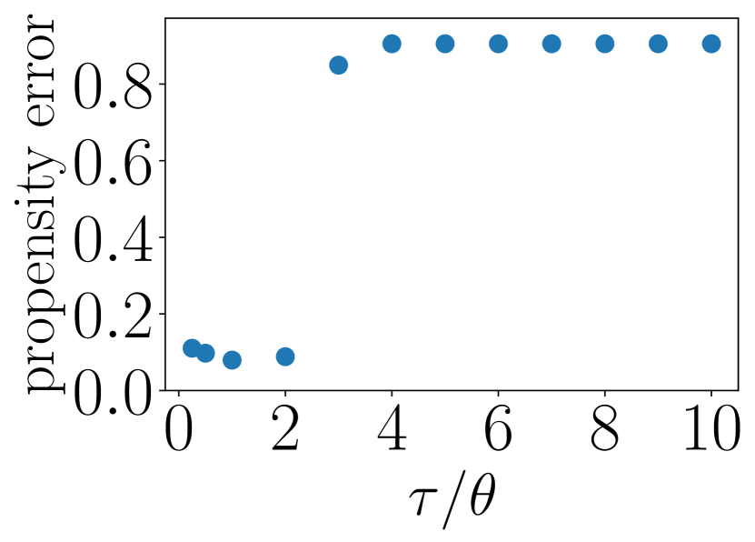
(a) sensitivity to $\tau$ when $\gamma/\alpha=1$

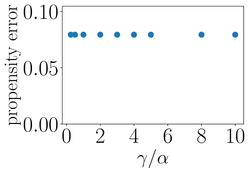
(b) sensitivity to $\gamma$ when $\tau/\theta=1$

Figure 6: Sensitivity of ConvexPE (Algorithm 1) to hyperparameters $\tau$ and $\gamma$.

The most important hyperparameter in NonconvexPE is the step size $t$. We show both the convergence and the change of propensity relative errors of NonconvexPE at several step sizes in Figure 7. We can see that the relative errors of propensity estimates steadily decrease at all step sizes at which the gradient descent converges. Also, the respective rankings of relative losses and propensity errors at different step sizes are the same across all iterations, indicating that the relative loss is a good surrogate metric for us to seek a good propensity estimate. Thus practitioners can select the largest step size at which NonconvexPE converges; it is $5\times 10^{-6}$ in our practice. This is much easier than the selection of $\tau$ in ConvexPE.

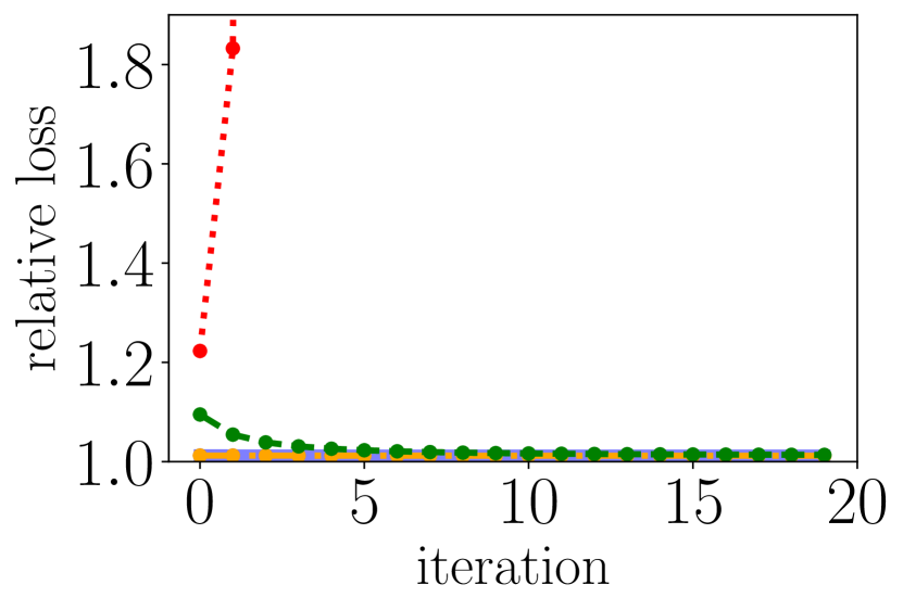
(a) change of relative loss

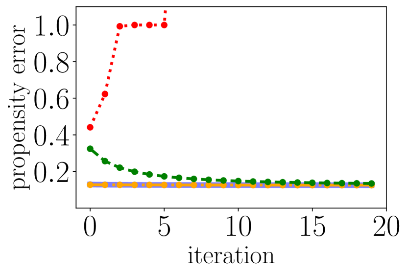
(b) change of propensity estimation error

[1pt]

Figure 7: Sensitivity of NonconvexPE (Algorithm 2) to step size $t$. Since the objective function is the logistic loss between the mask tensor $\Upomega$ and the parameter tensor $\mathscr{{A}}$, the relative loss in Figure 7(a) is the ratio of actual logistic loss to the best logistic loss computed from the true parameter tensor. Propensity error in Figure 7(b) is $\|\widehat{\mathscr{{P}}}-\mathscr{{P}}\|_{\mathrm{F}}/\|\mathscr{{P}}\|_{\mathrm{F}}$, the same as in the main paper.

References

- [ATT18] Anastasia Aidini, Grigorios Tsagkatakis, and Panagiotis Tsakalides. 1-bit tensor completion. Electronic Imaging, 2018(13):261–1, 2018.
- [AW17] Morteza Ashraphijuo and Xiaodong Wang. Fundamental conditions for low-cp-rank tensor completion. The Journal of Machine Learning Research, 18(1):2116–2145, 2017.
- [BM16] Boaz Barak and Ankur Moitra. Noisy tensor completion via the sum-of-squares hierarchy. In Conference on Learning Theory, pages 417–445, 2016.
- [CC70] J Douglas Carroll and Jih-Jie Chang. Analysis of individual differences in multidimensional scaling via an N-way generalization of “Eckart-Young” decomposition. Psychometrika, 35(3):283–319, 1970.
- [CT10] Emmanuel J Candès and Terence Tao. The power of convex relaxation: Near-optimal matrix completion. IEEE Transactions on Information Theory, 56(5):2053–2080, 2010.
- [CZ13] Tony Cai and Wen-Xin Zhou. A max-norm constrained minimization approach to 1-bit matrix completion. The Journal of Machine Learning Research, 14(1):3619–3647, 2013.
- [DK70] Chandler Davis and William Morton Kahan. The rotation of eigenvectors by a perturbation. iii. SIAM Journal on Numerical Analysis, 7(1):1–46, 1970.
- [DLDMV00] Lieven De Lathauwer, Bart De Moor, and Joos Vandewalle. A multilinear singular value decomposition. SIAM journal on Matrix Analysis and Applications, 21(4):1253–1278, 2000.
- [DPVDBW14] Mark A Davenport, Yaniv Plan, Ewout Van Den Berg, and Mary Wootters. 1-bit matrix completion. Information and Inference: A Journal of the IMA, 3(3):189–223, 2014.
- [GPY18] Navid Ghadermarzy, Yaniv Plan, and Ozgur Yilmaz. Learning tensors from partial binary measurements. IEEE Transactions on Signal Processing, 67(1):29–40, 2018.
- [GRY11] Silvia Gandy, Benjamin Recht, and Isao Yamada. Tensor completion and low-n-rank tensor recovery via convex optimization. Inverse Problems, 27(2):025010, 2011.
- [H+70] Richard A Harshman et al. Foundations of the PARAFAC procedure: Models and conditions for an “explanatory” multimodal factor analysis. 1970.
- [HKD20] David Hong, Tamara G Kolda, and Jed A Duersch. Generalized canonical polyadic tensor decomposition. SIAM Review, 62(1):133–163, 2020.
- [HN20] Longxiu Huang and Deanna Needell. Hosvd-based algorithm for weighted tensor completion. arXiv preprint arXiv:2003.08537, 2020.
- [JO14] Prateek Jain and Sewoong Oh. Provable tensor factorization with missing data. In Advances in Neural Information Processing Systems, pages 1431–1439, 2014.
- [KS13] Akshay Krishnamurthy and Aarti Singh. Low-rank matrix and tensor completion via adaptive sampling. In Advances in Neural Information Processing Systems, pages 836–844, 2013.
- [LM20] Allen Liu and Ankur Moitra. Tensor completion made practical. arXiv preprint arXiv:2006.03134, 2020.
- [MB18] Osman Asif Malik and Stephen Becker. Low-rank tucker decomposition of large tensors using tensorsketch. In Advances in Neural Information Processing Systems, pages 10096–10106, 2018.
- [MC19] Wei Ma and George H Chen. Missing not at random in matrix completion: The effectiveness of estimating missingness probabilities under a low nuclear norm assumption. In Advances in Neural Information Processing Systems, pages 14871–14880, 2019.
- [MHWG14] Cun Mu, Bo Huang, John Wright, and Donald Goldfarb. Square deal: Lower bounds and improved relaxations for tensor recovery. In International Conference on Machine Learning, pages 73–81, 2014.
- [NW12] Sahand Negahban and Martin J Wainwright. Restricted strong convexity and weighted matrix completion: Optimal bounds with noise. Journal of Machine Learning Research, 13(May):1665–1697, 2012.
- [Ose11] Ivan V Oseledets. Tensor-train decomposition. SIAM Journal on Scientific Computing, 33(5):2295–2317, 2011.
- [RY17] Ernest K Ryu and Wotao Yin. Proximal-proximal-gradient method. arXiv preprint arXiv:1708.06908, 2017.
- [SGL+19] Yiming Sun, Yang Guo, Charlene Luo, Joel Tropp, and Madeleine Udell. Low-rank tucker approximation of a tensor from streaming data. arXiv preprint arXiv:1904.10951, 2019.
- [T+15] Joel A Tropp et al. An introduction to matrix concentration inequalities. Foundations and Trends® in Machine Learning, 8(1-2):1–230, 2015.
- [THK10] Ryota Tomioka, Kohei Hayashi, and Hisashi Kashima. Estimation of low-rank tensors via convex optimization. arXiv preprint arXiv:1010.0789, 2010.
- [Tuc66] Ledyard R Tucker. Some mathematical notes on three-mode factor analysis. Psychometrika, 31(3):279–311, 1966.
- [WAA16] Wenqi Wang, Vaneet Aggarwal, and Shuchin Aeron. Tensor completion by alternating minimization under the tensor train (TT) model. arXiv preprint arXiv:1609.05587, 2016.
- [Wed72] Per-Åke Wedin. Perturbation bounds in connection with singular value decomposition. BIT Numerical Mathematics, 12(1):99–111, 1972.
- [XYZ17] Dong Xia, Ming Yuan, and Cun-Hui Zhang. Statistically optimal and computationally efficient low rank tensor completion from noisy entries. arXiv preprint arXiv:1711.04934, 2017.
- [YEG+18] Tatsuya Yokota, Burak Erem, Seyhmus Guler, Simon K Warfield, and Hidekata Hontani. Missing slice recovery for tensors using a low-rank model in embedded space. In Proceedings of the IEEE Conference on Computer Vision and Pattern Recognition, pages 8251–8259, 2018.
- [YWS15] Yi Yu, Tengyao Wang, and Richard J Samworth. A useful variant of the davis–kahan theorem for statisticians. Biometrika, 102(2):315–323, 2015.
- [YZGC18] Longhao Yuan, Qibin Zhao, Lihua Gui, and Jianting Cao. High-dimension tensor completion via gradient-based optimization under tensor-train format. arXiv preprint arXiv:1804.01983, 2018.
- [Z+19] Anru Zhang et al. Cross: Efficient low-rank tensor completion. The Annals of Statistics, 47(2):936–964, 2019.