Quantum quench dynamics in XY spin chain with ferromagnetic and antiferromagnetic interactions

Abstract

In this manuscript we investigate the one-dimensional anisotropic XY model with ferromagnetic and antiferromagnetic interactions, which gives more interesting phase diagrams and dynamic critical behaviors. By using quantum renormalization-group method, we find that there are three phases in the system: antiferromagnetic Ising phase ordered in “$x$ direction”, spin-fluid phase and ferromagnetic Ising phase ordered in “$y$ direction”. In order to study the dynamical critical behaviors of the system, two quantum quenching methods are used. In both cases, the concurrence, a measure of entanglement, oscillates periodically over time. We show that the periods are the same and can be used as a new order parameter for quantum phase transitions. For further discussion, we derive the scaling exponent, $\theta$, and correlation length exponent, $\nu$, from the scaling behavior of the evolution period.

I INTRODUCTION

As a kind of nonlocal correlation, quantum entanglement has attracted extensive attention in many study fields. In quantum information theory, it can be regarded as an essential resource for processing information that is impossible to achieve in classical information theory1 ; 2 ; 3 ; 4 . In condensed matter physics, it plays a key role in the study of quantum phase transition(QPT) which occurs at zero temperature and is induced by the changing of parameters in the Hamiltonian 5 ; 6 ; 7 .

In the past few years, the static properties between entanglement and the QPT in quantum many-body spin systems are studied widely. For example, the Ising, XY, and XXZ models are investigated by using quantum renormalization group(QRG) method. In these studies it was shown that the entanglement can be used as an order parameter to QPT and the critical exponents can be derived from its scaling behavior8 ; 9 ; 10 ; 11 ; 12 ; 13 ; 14 .

Recently as the advance in ultracold atomic, molecule experiments, and the development of ultrafast pulsed lasers15 ; 16 ; 17 ; 18 , there is a growing savor for studying the dynamics of quantum many-body spin systems19 ; 20 ; 21 ; 22 ; 23 . Among them, Jafari study the dynamics of the one-dimensional Ising model in transverse field by QRG method, and find that the characteristic time(at which the entanglement reaches its 1th maximum) can used to define the critical point19 . Hazzard et al. investigate XXZ spin system following a quantum quench which is easily to achieve experimentally and reveal that time evolution of correlation function manifests a nonperturbative dynamic singularity21 . Meng Qin et al. discuss the non-equilibrium evolution of quantum coherence in one-dimensional anisotropic XY model by giving an initial state arbitrarily and find that quantum coherence periodically fluctuates over time23 .

However, there are some open questions still need to answer. Can we study the dynamic critical behaviors of the quantum many-body spin systems deeply by quantum quench? Can we find a new order parameter for quantum phase transition? If there are new order parameters, what critical information can we derive from it? Based on these questions, we study the dynamics of quantum entanglement for one-dimensional ferromagnetic-antiferromagnetic spin-$1/2$ XY system. The organization of this manuscript is as follows. In Sec. II the phase diagram of the system is discussed by QRG method. In Sec. III the dynamic evolution of the system by two quantum quenching methods is studied. The relation between the evolution period of entanglement and the QPT is investigated in sec. IV and the summary is given in the last section.

II QRG METHOD AND PHASE DIAGRAM

The XY model was initially studied by E. Lieb and since then it was widely investigated10 ; 11 ; 23 ; 24 ; 25 ; 26 ; 27 . In this manuscript we go on to study the XY spin chain with ferromagnetic and antiferromagnetic interactions. The Hamiltonian of the system on a periodic chain with $N$ sites reads

$$H=\frac{1}{4}\underset{i=1}{\overset{N}{\sum}}\left(J_{x}\sigma_{i}^{x}\sigma_{i+1}^{x}-J_{y}\sigma_{i}^{y}\sigma_{i+1}^{y}\right),$$ (1)

where $\sigma_{i}^{\alpha}\left(\alpha=x,y\right)$ are Pauli operators at site $i$,$\ J_{x}=$ $J\left(1+\gamma\right)$ and $J_{y}=J\left(1-\gamma\right)\left(J>0\right)$ are exchange coupling constants, in which $-1\leq\gamma\leq 1$ is the anisotropy parameter.

QRG method is well suited to solve many-body systems, and they are conceptually easy to be extended to the higher dimensions. Next, we study the phase diagram of this system by Kadanoff’s block QRG method28 ; 29 ; 30 ; 31 . Its main idea is to reduce the degrees of freedom until a manageable situation is reached. A brief introduction to the steps of QRG is follows8 ; 9 ; 10 ; 11 . First and foremost is that the lattice are divided into blocks in a reasonable way. Secondly, the block Hamiltonian is diagonalized exactly. After that, the low-lying eigenstates of all the blocks are used to construct projection operatorscons. By it the full Hamiltonian is projected onto these eigenstates, which gives the effective Hamiltonian. Final, the QRG equations are obtained by calculating and comparing between previous Hamiltonian and the effective one. The advantage of the QRG method is not only to simplify the system but also to keep the low energy spectrum of the system invariant, which is very important to explore quantum issues with zero temperature.

Above one has briefly introduced the steps of QRG, and will apply it to our system. One find that three sites as a block is most reasonable, and based on Kadanoff’s block approach we write the Eq. (1) as

$$H=H^{\text{B}}+H^{\text{BB}},$$ (2)

where $H^{\text{B}}$ is block Hamiltonian and $H^{\text{BB}}$ is interblock Hamiltonian. The specific forms of $H^{\text{B}}$ and $H^{\text{BB}}$ are

$$H^{\text{B}}=\sum_{I=1}^{N\diagup 3}h_{I}^{\text{B}},$$ (3)

in which

$$h_{I}^{\text{B}}=\left[J_{x}\left(\sigma_{I,1}^{x}\sigma_{I,2}^{x}+\sigma_{I,2}^{x}\sigma_{I,3}^{x}\right)-J_{y}\left(\sigma_{I,1}^{y}\sigma_{I,2}^{y}+\sigma_{I,2}^{y}\sigma_{I,3}^{y}\right)\right]/4,$$ (4)

$$H^{\text{BB}}=\sum_{I=1}^{N\diagup 3}\left(J_{x}\sigma_{I,3}^{x}\sigma_{I+1,1}-J_{y}\sigma_{I,3}^{y}\sigma_{I+1,1}^{y}\right)/4,$$ (5)

where $\sigma_{I,j}^{\alpha}\left(\alpha=x,y\right)$ refer to the Pauli matrix at site $j$ of the block labeled by $I.$

In the space spanned by $\left\{\left|\uparrow\uparrow\uparrow\right\rangle,\left|\uparrow\uparrow\downarrow\right\rangle,\left|\uparrow\downarrow\uparrow\right\rangle,\left|\uparrow\downarrow\downarrow\right\rangle,\left|\downarrow\uparrow\uparrow\right\rangle,\left|\downarrow\uparrow\downarrow\right\rangle,\left|\downarrow\downarrow\uparrow\right\rangle,\left|\downarrow\downarrow\downarrow\right\rangle\right\}$ $\left(\text{where }\left|\uparrow\right\rangle\ \text{and }\left|\downarrow\right\rangle\text{\ represent the eigenstates of }\sigma^{z}\right),$ the block Hamiltonian can be exactly diagonalized and the degenerate ground states can be obtained as

$$\left|\Phi_{0}\right\rangle=\frac{1}{2\sqrt{1+\gamma^{2}}}\left(-\sqrt{1+\gamma^{2}}\left|\uparrow\uparrow\downarrow\right\rangle+\sqrt{2}\gamma\left|\uparrow\downarrow\uparrow\right\rangle-\sqrt{1+\gamma^{2}}\left|\downarrow\uparrow\uparrow\right\rangle+\sqrt{2}\left|\downarrow\downarrow\downarrow\right\rangle\right),$$ (6)

$$\left|\Phi_{0}^{{\acute{}}}\right\rangle=\frac{1}{2\sqrt{1+\gamma^{2}}}\left(-\sqrt{2}\left|\uparrow\uparrow\uparrow\right\rangle-\sqrt{2}\gamma\left|\downarrow\uparrow\downarrow\right\rangle+\sqrt{1+\gamma^{2}}\left|\uparrow\downarrow\downarrow\right\rangle+\sqrt{1+\gamma^{2}}\left|\downarrow\downarrow\uparrow\right\rangle\right).$$ (7)

The degenerate ground states of all blocks are used to build projection operator $T_{0}$ where $T_{0}=\mathop{\textstyle\prod}\nolimits_{I=1}^{N/3}T_{0}^{I},$ and specific form of $T_{0}^{I}$ is

$$T_{0}^{I}=\left|\Uparrow\right\rangle_{I}\left\langle\Phi_{0}\right|+\left|\Downarrow\right\rangle_{I}\left\langle\Phi{\acute{}}_{0}\right|,$$ (8)

in which $\left|\Uparrow\right\rangle_{I}$ and $\left|\Downarrow\right\rangle_{I}$ are renamed base kets in the effective subspace. Projection operators can be used to associate effective Hamiltonian with initial one in the following form

$$H^{\text{eff}}=T^{{\dagger}}H^{\text{B}}T+T^{{\dagger}}H^{\text{BB}}T.$$ (9)

By calculating and comparing with Eq. (1), we get the effective one as

$$H^{\text{eff}}=\underset{I=1}{\overset{N/3}{\sum}}\left[J_{x}^{{}^{\prime}}\sigma_{I}^{x}\sigma_{I+1}^{x}-J_{y}^{\prime}\sigma_{I}^{y}\sigma_{I+1}^{y}\right]/4$$ (10)

with

$$J_{x}^{{}^{\prime}}=J^{\prime}\left(1+\gamma^{{}^{\prime}}\right),J_{y}^{\prime}=J^{\prime}\left(1-\gamma^{{}^{\prime}}\right),$$ (11)

in which

$$J^{{}^{\prime}}=J\frac{3\gamma^{2}+1}{2\left(1+\gamma^{2}\right)},\gamma^{{}^{\prime}}=\frac{\gamma^{3}+3\gamma}{3\gamma^{2}+1}.$$ (12)

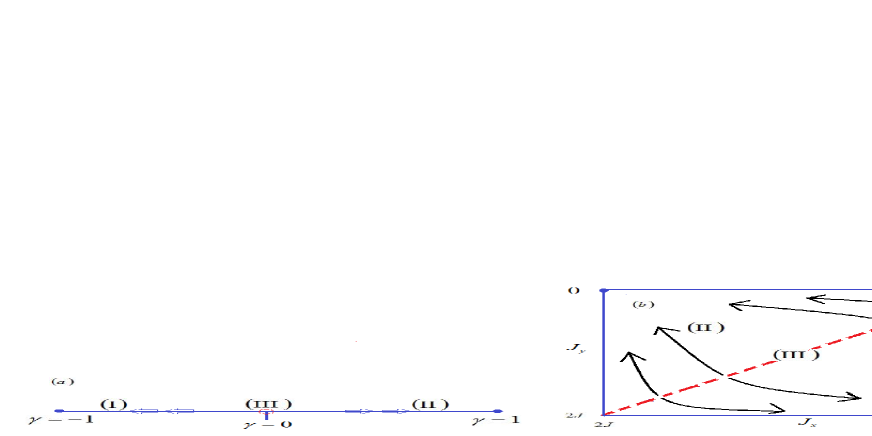
Figure 1: $\left(\text{Coloronline}\right)$ Phase diagram of the one-dimensional ferromagnetic-antiferromagnetic spin-1/2 XY system. Arrows show running of couplings under QRG. Filled circles represent stable fixed points and open circle is unstable fixed point and the red dotted line corresponds to the open circle.  Phase$\left(\text{I}\right)$ is ferromagnetic Ising phase ordered in “y direction”, $\left(\text{II}\right)$ represents antiferromagnetic Ising phase ordered in “x direction”, and $\left(\text{III}\right)$ is spin-fluid phase.

Above equation is the ultimate results of QRG and from it we can get a lot of information of the system. Based on it, we plot the the phase diagrams of the system in Fig. 1 and we will give a simple explanation following. At zero temperature, a phase transition occurs upon relative variation of the parameters in the Hamiltonian32 . In this system the exchange coupling constant $J_{x}$ makes the spins staggered arrangement along the “x direction” i.e., makes the system in antiferromagnetic Ising phase. The exchange coupling constant $-J_{y}$ makes all spins in the “positive or negative direction of y” i.e., makes the system in ferromagnetic Ising phase. The competition between $J_{x}$ and $J_{y}$ leads to the QPT between antiferromagnetic Ising phase and ferromagnetic one. An advantage of this model is that the competition can be also described by a single $\gamma$. From Eq. (1) we can see that when $\gamma$ determined $J_{x}$ and $J_{y}$ can be determined simultaneously. So the QPT can be described by $J_{x}$ and $J_{y}$ or $\gamma.$

For simplicity, let’s analyze the phase diagram of the system with a single gama, and correspond to a two-dimensional parameter space. By solving $\gamma^{{}^{\prime}}=\gamma$, we get the fixed points in which the stable one are $\gamma=\pm 1$ and the unstable one is $\gamma=0.$ At $\gamma=1,$ the system is in the antiferromagnetic Ising phase ordered in “x direction”. The $\gamma=-1$ corresponds to ferromagnetic Ising phase ordered in “$y$ direction”. At $\gamma=0,$ the spins can point to either “x directions” or “y directions” due to the competition between $J_{x}$ and $J_{y}$ is the same. For this point,the system is in the spin-fluid phase, because the most disordered state but largest entanglement which will show in in the Sec.III33 . Other points flow to corresponding stable fixed point at the thermodynamic limit, which tells us that the $\gamma_{c}=0$ is the transition point from ferromagnetic Ising phase $\left(0>\gamma\geqslant-1\right)$ to the spin-fluid phase $\left(\gamma=0\right)$ or from spin-fluid phase to the antiferromagnetic Ising phase $\left(1\geq\gamma>0\right).$

III QUENCH DYNAMICS

There are many interesting and unknown things in dynamic critical properties of quantum many-body spin systems. Exploring these things is important to understand the nature of quantum systems. In this section, we study the dynamic critical behaviors of entanglement in ferromagnetic-antiferromagnetic spin-1/2 XY system by two quantum quenching methods(1. closing the external field suddenly; 2. changing the coupling constant suddenly) and we use concurrence to measure entanglement 34 ; 35 ; 36 ; 37 .

Quench 1: From the experimental point of view, one can make the system with Hamiltonian

$$H_{1}=\sum_{i=1}^{N}\left(J_{x}\sigma_{i}^{x}\sigma_{i+1}^{x}-J_{y}\sigma_{i}^{y}\sigma_{i+1}^{y}+h\sigma_{i}^{z}\right)/4$$

in the ground state by low temperature. When the system is in the ground state, we can realize quench by removing transverse field, $h$, abruptly at time $t=0$. In short, the system with Hamiltonian $H$ begins to evolve from ground state of the Hamiltonian $H_{1}$. All in all, this method is easy to implement.

In the process of dynamics, it is difficult to calculate the concurrence of large system directly. Next we first calculate the concurrence of the three-site system and then investigate it in a large one by QRG method. The calculation process is as follows. The density matrix of the three-site system before quenching needs to be given first by $\rho_{1}\left(0\right)=\left|\varphi_{{}_{1}}\right\rangle\left\langle\varphi_{{}_{1}}\right|$ in which $\left|\varphi_{{}_{1}}\right\rangle$ =$\left|\downarrow\downarrow\downarrow\right\rangle$˙Then the density matrix at time $t$ can be gotten by $\rho\left(t\right)=U\left(t\right)\rho\left(0\right)U^{{\dagger}}\left(t\right)$ where $U\left(t\right)=e^{-iHt}$ is unitary operator. In the space which has been given in Sec. II, the unitary operator is obtained as

$$U\left(t\right)=\left(\begin{array}[]{cccccccc}a&0&0&b&0&c&b&0\\ 0&d&e&0&f&0&0&b\\ 0&e&g&0&e&0&0&c\\ b&0&0&d&0&b&f&0\\ 0&f&e&0&d&0&0&b\\ c&0&0&b&0&g&e&0\\ b&0&0&f&0&e&d&0\\ 0&b&c&0&b&0&0&a\end{array}\right),$$ (13)

in which we consider $J$=1 and the specific values are as follows

$$a = \frac{\gamma^{2}+\cos\omega t}{1+\gamma^{2}},b=-\frac{i\sin\omega t}{\sqrt{2\left(1+\gamma^{2}\right)}},$$

$$c = \frac{\gamma\left(-1+\cos\omega t\right)}{1+\gamma^{2}},d=\left(\cos\frac{\omega t}{2}\right)^{2},$$

$$e = -\frac{i\gamma\sin\omega t}{\sqrt{2\left(1+\gamma^{2}\right)}},f=\frac{1}{2}\left(-1+\cos\omega t\right),$$

$$g = \frac{1+\gamma^{2}\cos\omega t}{1+\gamma^{2}},\omega=\frac{\sqrt{1+\gamma^{2}}}{\sqrt{2}}.$$

After get the density matrix at time t, we can get pairwise concurrence by tracing the degrees of freedom of one site. Without loss generality, we trace site 2 and the reduced density matrix for sites 1 and 3 at time $t$ can be obtained as

$$\rho_{1}\left(\gamma,t\right)=\left(\begin{array}[]{cccc}k&0&0&q\\ 0&m&m&0\\ 0&m^{\ast}&m&0\\ q^{\ast}&0&0&p\end{array}\right),$$ (14)

where

$$k = \frac{\left(\gamma^{2}+\cos\omega t\right)^{2}}{\left(1+\gamma^{2}\right)^{2}},$$

$$q = \frac{\gamma\left(-1+\cos\omega t\right)\left(\gamma^{2}+\cos\omega t\right)}{\left(1+\gamma^{2}\right)^{2}},$$

$$m = \frac{\left(\sin\omega t\right)^{2}}{2+2\gamma^{2}},$$

$$p = \frac{\gamma^{2}\left(-1+\cos\omega t\right)^{2}}{\left(1+\gamma^{2}\right)^{2}}.$$

The reduced density matrix has X-state formation due to $k+2m+p=1,$ $m^{\ast}=m,$ and $q^{\ast}=q$. Based on this, we get the concurrence as38

$$C_{1}\left(\gamma,t\right)=2\max\left\{0,m-\sqrt{kp},\left|q\right|-m\right\}.$$ (15)

Quench 2: The system is initially in the ground state of the Hamiltonian $H_{2}=\sum_{i=1}^{N}\left[J_{x}\sigma_{i}^{x}\sigma_{i+1}^{x}+J_{y}\sigma_{i}^{y}\sigma_{i+1}^{y}\right]/4$ and then the $J_{y}$ is changed suddenly to $-J_{y}$ at $t=0$. The initial state is $\left|\varphi_{2}\right\rangle=\frac{1}{2}\left(-\left|\uparrow\uparrow\downarrow\right\rangle+\frac{\sqrt{2}}{\sqrt{1+\gamma^{2}}}\left|\uparrow\downarrow\uparrow\right\rangle-\frac{1}{\sqrt{2}}\left|\downarrow\uparrow\uparrow\right\rangle+\frac{\sqrt{2}\gamma}{\sqrt{1+\gamma^{2}}}\left|\downarrow\downarrow\downarrow\right\rangle\right).$ Similarly, the reduced density matrix for sites 1 and 3 can be gotten as

$$\rho_{2}\left(\gamma,t\right)=\left(\begin{array}[]{cccc}x&0&0&s\\ 0&z&z&0\\ 0&z^{\ast}&z&0\\ s^{\ast}&0&0&y\end{array}\right),$$ (16)

where

$$s = -\frac{\gamma-10\gamma^{3}+\gamma^{5}-4\gamma\left(-1+\gamma^{2}\right)\cos\omega t+\gamma\left(-1+\gamma^{2}\right)^{2}\cos 2\omega t-2i\left(-1+\gamma^{2}\right)\left(1+\gamma^{2}\right)^{2}\sin\omega t}{4\left(1+\gamma^{2}\right)^{3}},$$

$$x \frac{2-3\gamma^{2}+8\gamma^{4}+\gamma^{6}+\gamma^{2}\left(-1+\gamma^{2}\right)\left(-8\cos\omega t-\left(-1+\gamma^{2}\right)\cos 2\omega t\right)}{4\left(1+\gamma^{2}\right)^{3}},$$ =

$$y = \frac{1+8\gamma^{2}-3\gamma^{4}+2\gamma^{6}+8\gamma^{2}\left(-1+\gamma^{2}\right)\cos\omega t-\left(-1+\gamma^{2}\right)^{2}\cos 2\omega t}{4\left(1+\gamma^{2}\right)^{3}},$$

$$z = \frac{1+6\gamma^{2}+\gamma^{4}+\left(-1+\gamma^{2}\right)\cos 2\omega t}{8\left(1+\gamma^{2}\right)^{2}},$$

and the concurrence can be obtained as

$$C_{2}\left(\gamma,t\right)=\text{2Max}\left\{0,z-\sqrt{xy},\left|s\right|-z\right\}.$$ (17)

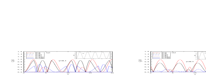
Figure 2: $\left(\text{Coloronline}\right)$ Evolution of concurrences over the time under different QRG steps at $\gamma=0.1$. $\left(\text{a}\right)$ and $\left(\text{b}\right)$ correspond to the first and second kind of quantum quench respectively. Inset: Concurrences of different size of the system coincide with each other at the critical$\ \left(\gamma=0\right).$

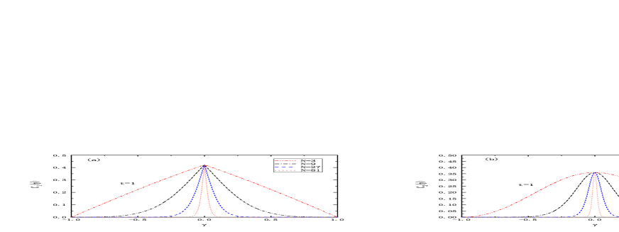
Figure 3: $\left(\text{Coloronline}\right)$ Variation of the concurrences versus $\gamma$ after both kinds of quantum quench at $t=1.$ As the size of the system increases, the concurrences show singular behavior at $\gamma=0$ which shows that the QPT occurs here.

For more intuitive analysis, we first show the evolution of concurrences over the time under QRG steps in the Fig. 2. (a) describes the first quench method, (b) describes the second one. From Fig. 2$\left(\text{a}\right),$ we find that the concurrence periodically oscillates from zero. This may be caused by the constant fluctuation between the ground state of the system before quenching and after quenching. As the size of the system increases, the concurrence decreases gradually and disappears in a large system. The reason for this is that any points except the critical point flow to a stable fixed point $\left(\text{after\ enough\ iterations}\right)$ and the state corresponding to it can be separated into the product of subsystems. Moreover, the concurrence of different-length chains coincide with each other at the critical point $\left(\text{Fig. 2, inset}\right)$, because that the correlation length diverges at this point. From Fig. 2$\left(\text{b}\right)$, we can see that the concurrence periodically oscillates from no-zero values, which indicates that the initial state is entangled. Comparing the two figures,we can see that the performance of concurrence are different when system is finite,but the characteristic is consistent under the thermodynamic limit.In other words,different quenching methods do not affect the critical phenomenon,which can also be shown by the scaling behavior of the same period later.

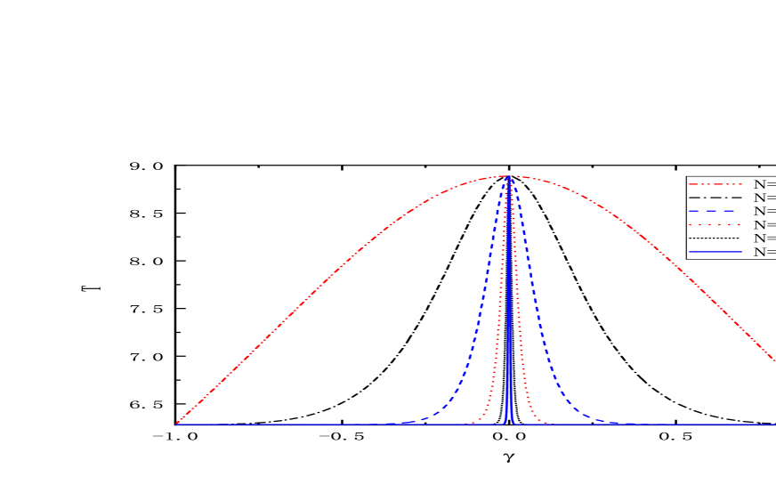
Figure 4: $\left(\text{Coloronline}\right)$ Evolution period $T$ as a function of $\gamma$ for different QRG steps. Similar to concurrence, the period $T$ shows singular behavior at $\gamma=0.$

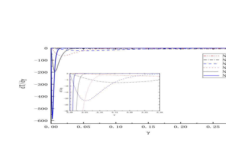
Figure 5: $\left(\text{Coloronline}\right)$ First derivation of the evolution period $T$ with respect to the $\gamma$ for different size of the system. In the figure, we only give the $\gamma\geq 0$, because the $T$ is an even function of $\gamma.$

Figure 6: Scaling behavior of the system, ln$\left|\left(dT/d\gamma\right)_{\min}\right|$ with the logarithm of the system size $N.$ Inset: Scaling of the position $\left(\gamma_{m}\right)$ of $\left(dT/d\gamma\right)_{\min}$ for different-length chains.

When time is given the concurrences versus $\gamma$ are plotted in Fig. 3. For the both kinds of quantum quench, it is found that the plots under different QRG steps cross each other at the critical point which is due to that this point is fixed point. In the thermodynamic limit, the concurrences develop two saturated values, one is non-zero corresponding to the ordered phase and one is zero corresponding to the disordered phase.

IV EVOLUTION PERIOD AND QPT

Above we find that the concurrences periodically oscillate over the time for both kinds of quantum quench and we deduce that the periods is the same from Eq. $\left(15\right)$ and Eq. $\left(17\right).$The evolution period, $T,$ of three-site system is given as

$$T=2\sqrt{2}\pi/\left(\sqrt{1+\gamma^{2}}\right),$$ (18)

and we will study it in a large system with renormalized coupling constants.

We expect that the evolution period is a new order parameter, because it does not depend on the quench methods. $T$ with $\gamma$ for different system sizes, $N,$ is plotted in Fig. 4. Similar to concurrence, the period $T$ tends to two different values in the thermodynamic corresponding to the ordered phase and disordered phase respectively.

For further discussion, we plot the first derivative of the evolution period, $dT/d\gamma,$ in Fig. 5. The derivative of the $T$ diverges at $\gamma_{c}=0$ under the thermodynamic limit, which shows that a second-order QPT occurs at this point, which can also be proven by the scaling behavior of $\left|\left(dT/d\gamma\right)_{\min}\right|$ . We have derived the scaling behavior of $\left|\left(dT/d\gamma\right)_{\min}\right|$ versus N and displayed it in Fig. 6 which shows a linear behavior of ln$\left|\left(dT/d\gamma\right)_{\min}\right|$ versus lnN. The scaling behavior is $\left|\left(dT/d\gamma\right)_{\min}\right|\sim N^{\theta},$ with exponent $\theta=1$. The exponent $\theta$ is related to the correlation length exponent closed to the critical point and we can give a simple derivation process here. In the vicinity of $\gamma_{c}=0$, the correlation length exponent, $\nu,$ gives the behavior of correlation length, that is $\xi\sim\left|\gamma-\gamma_{c}\right|^{-\nu}.$ Under the $n$th QRG steps, the correlation length can be written as $\xi_{\left(n\right)}=\xi/3^{n}\sim\left|\gamma_{\left(n\right)}-\gamma_{c}\right|^{-\nu}$ where $\gamma_{\left(n\right)}$ is renormalized anisotropy parameter and dividing it to $\xi\sim\left|\gamma-\gamma_{c}\right|^{-\nu}$ gives $\left|\left(d\gamma_{n}/d\gamma\right)\right|_{\gamma_{c}}\sim N^{1/\nu}.$ We can give $\left|\left(dT/d\gamma\right)\right|_{\min}\sim\left|\left(d\gamma_{n}/d\gamma\right)\right|_{\gamma_{c}}$ since the position of the minimum $\left(\gamma_{\min}\right)$ tends toward the $\gamma_{c}$ as $\gamma_{\min}=\gamma_{c}+N^{-1}$ (Fig. 6, inset). To summarize the above derivation, we can get $\left|\left(dT/d\gamma\right)\right|_{\min}\sim N^{\theta}\sim\left|\left(d\gamma_{n}/d\gamma\right)\right|_{\gamma_{c}}\sim N^{1/\nu}$ which implies that $\nu=1/\theta$8 . The correlation length can be given as $\xi\sim\left(\gamma-\gamma_{c}\right)^{-1},$ which shows that the correlation length diverges at $\gamma_{c}=0.$

V
SUMMARY

The phase diagram and the dynamic critical behaviors of the concurrence in one-dimensional ferromagnetic-antiferromagnetic spin-1/2 XY system are studied in this manuscript. By the competition analysis between $J_{x}$ and $J_{y},$ the phases at the fixed points are obtained. The phase diagram of the system is given base on renormalization equation. We discuss the dynamics of the concurrences by both kinds of quantum quench which is easy to achieve experimentally and we find that the concurrences periodically oscillate over the time. The periods are the same and can be seen as order parameter to QPT. Finally, we get the correlation length exponent by analyzing the scaling behavior of the evolution period. The correlation length exponent equals to one, which indicates that the correlation length diverges at $\gamma_{c}=0$.

ACKNOWLEDGMENTS

This work is supported by the National Natural Science Foundation of China under Grants NO. 11675090, NO. 11505103, and NO. 11847086. Z.W. would like to thank Zhong-Qiang Liu, Yong-Yang Liu, Xiao-Hui Jiang, Qi-Ming Wang, Li-Yuan Wang, and Pan-Pan Zhang for fruitful discussions and useful comments.

References

- (1) M. A. Nielsen and I. L. Chuang, Quantum Computation and Quantum Communication(Cambridge University Press, Cambridge, 2000).
- (2) J. Preskill, “Lecture notes for ph219/cs219”, (2001).
- (3) V. Vedral, Rev. Mod. Phys. 74, 197 (2002).
- (4) T. Nishioka, Rev. Mod. Phys. 90, 035007 (2018).
- (5) G. Vidal, J. I. Latorre, E. Rico, and A. Kitaev, Phys. Rev. Lett. 90, 227902 (2003).
- (6) A. Kitaev, and J. Preskill, Phys. Rev. Lett. 96, 110404 (2006).
- (7) S. Sachdev, Quantum Phase Transitions(Cambridge University Press, Cambridge, 2000).
- (8) M. Kargarian, R. Jafari, and A. Langari, Phys. Rev. A 76, 060304(R) (2007).
- (9) R. Jafari, M. Kargarian, A. Langari, and M. Siahatgar, Phys. Rev. B 78, 214414 (2008).
- (10) F. W. Ma, S. X. Liu, and X. M. Kong, Phys. Rev. A 83, 062309 (2011).
- (11) F. W. Ma, S. X. Liu, and X. M. Kong, Phys. Rev. A 84, 042302 (2011).
- (12) M. Kargarian, R. Jafari, and A. Langari, Phys. Rev. A 77, 032346 (2008).
- (13) M. Kargarian, R. Jafari, and A. Langari, Phys. Rev. A 79, 042319 (2009).
- (14) Y. L. Xu, X. M. Kong, Z. Q. Liu, and C. C. Yin, Rev. A 95, 042327 (2017).
- (15) M. Greiner, O. Mandel, T. Esslinger, T. W. Hansch, and I. Bloch, Nature (London) 415, 39 (2002).
- (16) C. Regal, Ph.D. thesis (University of Colorado, Boulder, 2006).
- (17) I. Bloch, J. Dalibard, and W. Zwerger, Rev. Mod. Phys. 80, 885 (2008).
- (18) N. Gedik, D. S. Yang, G. Logvenov, I. Bozovic, and A. H. Zewail, Science 316, 425 (2007).
- (19) R. Jafari, Phys. Rev. A 82, 052317 (2010).
- (20) C. Karrasch, and D. Schuricht, Phys. Rev. B 87, 195104 (2013).
- (21) K. R. A. Hazzard, M. van den Worm, M. Foss-Feig, S. R. Manmana, E. G. Dalla Torre, T. Pfau, M. Kastner, and A. M. Rey, Phys. Rev. A 90, 063622 (2014).
- (22) S. Campbell, Phys. Rev. B 94, 184403 (2016).
- (23) M. Qin, Z. Z. Ren, and X. Zhang, Phys. Rev. A 98, 012303 (2018).
- (24) E. Lieb, T. Schultz, and D. Mattis, Ann. Phys. (NY) 16, 407 (1961).
- (25) R. Gupta, J. Delapp, G. G. Batrouni, G. C. Fox, C. F. Baillie, and J. Apostolakis, Phys. Rev. Lett. 61, 1996 (1988).
- (26) P. Olsson, PhyS. Rev. Lett. 75, 2758 (1995).
- (27) A. Langari, Rev. B 69, 100402 (2004).
- (28) K. G. Wilson, and J. Kogut, Phys. Rep. 12, 75 (1974).
- (29) J. Polchinski, Nucl. Phys. B. 231, 269 (1984).
- (30) O. J. Rosten, Phys. Rep. 511, 177 (2012).
- (31) U. C. Tauber, Nucl. Phys. B 228, 7 (2012).
- (32) G. J. Jin, D. Fen, Progress. In. Physics 29, 1000-0542 (2009).
- (33) L. Balents, Nature (London) 464, 199 (2010).
- (34) W. K. Wootters, Phys. Rev. Lett. 80, 2245 (1998).
- (35) A. Polkovnikov, K. Sengupta, A. Silva, and M. Vengalattore, Rev. Mod. Phys. 83, 863 (2011).
- (36) R. Dorner, J. Goold, C. Cormick, M. Paternostro, and V. Vedral, Phys. Rev. Lett. 109, 160601 (2012).
- (37) M. Heyl, Phys. Rev. Lett. 110, 135704 (2013).
- (38) T. Yu, and J. H. Eberly, Quantum. Inf. Comput. 7, 459 (2007).