The Sun: light dark matter and sterile neutrinos

Abstract

Next-generation experiments allow for the possibility to testing the neutrino flavor oscillation model to very high levels of accuracy. Here, we explore the possibility that the dark matter in the current universe is made of two particles, a sterile neutrino and a very light dark matter particle. By using a 3+1 neutrino flavor oscillation model, we study how such a type of dark matter imprints the solar neutrino fluxes, spectra, and survival probabilities of electron neutrinos. The current solar neutrino measurements allow us to define an upper limit for the ratio of the mass of a light dark matter particle $m_{\phi}$ and the Fermi constant $G_{\phi}$, such that $G_{\phi}/m_{\phi}$ must be smaller than $10^{30}\;G_{\rm F}eV^{-1}$ to be in agreement with current solar neutrino data from the Borexino, Sudbury Neutrino Observatory, and Super-Kamiokande detectors. Moreover, for models with a very small Fermi constant, the amplitude of the time variability must be lower than $3\%$ to be consistent with current solar neutrino data. We also found that solar neutrino detectors like Darwin, able to measure neutrino fluxes in the low energy-range with high accuracy, will provide additional constraints to this class of models that complement the ones obtained from the current solar neutrino detectors.

1. Introduction

The origin of dark matter has been a fundamental problem in physics for almost six decades, during which most of the proposed solutions assumed that a single massive particle that interacts weakly with baryons makes all the dark matter observed in the universe (e.g., Wang et al., 2016). Recently, research has emerged where more sophisticated solutions have been proposed to solve the dark matter problem. One of these is the possibility of the dark matter being a composite of two light particles: a light dark matter (LDM) particle $\phi$ and a sterile neutrino $\nu_{s}$.

The existence of such an LDM field can by identified with a dilation field of an extradimensional extension of the Standard Model or/and a CP-violating pseudo-Goldstone boson of a spontaneously broken global symmetry. For some of these models, $\phi$ couples to the Standard Model fields, and as such it induces periodic time variation in particle masses and couplings. In such theories the gauge invariance suggests that the $\phi$ should possess an identical coupling constant to charged leptons, in which case scalar interactions with the electrons provide a good opportunity for detection through atomic clocks (e.g., Arvanitaki et al., 2016), accelerometers (e.g., Arvanitaki et al., 2018), and gravitational wave detectors (e.g., Lopes and Silk, 2014; Graham et al., 2016).

Similarly, this $\phi$ field can couple to neutrinos. Once again, these types of interactions generically result in time-varying corrections to the neutrino masses, neutrino mass differences, and mixing angles, which can be searched for in the neutrino flux signals on present and future experimental neutrino detectors (Aharmim et al., 2013; Abe et al., 2016; Borexino Collaboration et al., 2018; Aalbers et al., 2020). If $\phi$ couples weakly to the neutrinos, over a large range of masses, it can significantly modify the neutrino oscillations probabilities leading to a distorted survival electron neutrino probability function (Berlin, 2016; Krnjaic et al., 2018).

The motivation for such a model comes from the possibility of this composite particle physics model resolving two observational problems:

1. The classical cold dark matter model leads to several inconsistencies with the cosmological observational data, such as the missing satellite problem and the cusp problem (e.g., Primack, 2009). Light dark matter resolves such problems if dark matter is totally or partially made of light scalar particles with a mass of the order of $10^{-22}{\rm eV}$ (Hu et al., 2000; Peebles, 2000). In hierarchical models of structure formation, such type of dark matter is able to explain the flatness observed on the profiles of the distribution of gas and stars in halos and filaments (Mocz et al., 2019).

2. Although the standard three neutrino flavor model produces a reasonable good global fit to all the neutrino data (Esteban et al., 2019), there are now many hints that point out to the possibility of the existence of a fourth neutrino. This one does not have any other interaction than gravity and for that reason is known as a sterile neutrino (Diaz et al., 2019). It was found that a flavor oscillation model made of the 3 active neutrinos plus a sterile neutrino could explain some of the observed anomalies found on the Short baseline neutrino oscillation experiments (Giunti et al., 2012, 2013), Liquid Scintillator Neutrino Detector (Aguilar et al., 2001), and MiniBooNE Short-Baseline Neutrino Experiment (MiniBooNE Collaboration et al., 2018), as well as the anomalies related with GALLEX and SAGE solar-neutrino detectors – the so-called Gallium anomalies (Kostensalo et al., 2019). For instance, Kostensalo et al. (2019) found that the data favour a $3+1$ neutrino flavor model with $m_{4}=\;1.1eV$ and mixing matrix element $U_{e4}=0.11$.

One possibility to resolve both problems (neutrino anomalies and structure formation) is to consider that dark matter is made of a light scalar field that couples to a sterile neutrino (e.g., Farzan, 2019). The interactions of $\phi$ and $\nu_{s}$ could impede the oscillations in the universe and thereby improve the agreement between the structure formation and cosmological observations (e.g., Dasgupta and Kopp, 2014; Hannestad et al., 2014).

If such $\phi$ and $\nu_{s}$ particles exist today, they were produced abundantly in the early universe. For instance, sterile neutrinos can be produced via mixing with active neutrinos (Dodelson and Widrow, 1994), in some scenarios such neutrino production is being enhanced by the oscillations between active and sterile neutrinos (Bezrukov et al., 2019, 2020; de Gouvêa et al., 2020) or by the lepton asymmetry (Shi and Fuller, 1999). The production of light dark matter can take many forms, such as vector bosons by parametric resonance production (Dror et al., 2019). For instance, some models predict a sterile neutrino abundance of $\Omega_{s}^{2}h^{2}=0.12\left({\sin^{2}{(2\theta_{s})}}/{3.5\times 10^{-9}}\right)\left({m_{\nu_{s}}}/{7keV}\right)$ where $m_{\nu_{s}}$ and $\theta_{s}$ is the sterile neutrino mass and mixing angle (Kusenko, 2009). For the light dark matter field some authors obtained $\Omega_{\phi}^{2}=0.1\left({a_{o}}/{10^{17}\;{\rm GeV}}\right)^{2}\left({m_{a}}/{10^{-22}\;{\rm eV}}\right)^{1/2}$, where $a_{o}$ is a parameter that relates to the initial misalignment angle of the axion, and $m_{a}$ is the axion mass (Hui et al., 2017; Niemeyer, 2019). Conveniently, we will assume that in the present-day universe the total dark matter abundance is given by

$$\Omega_{\rm DM}h^{2}=\Omega_{\phi}^{2}h^{2}+\Omega_{\nu_{s}}^{2}h^{2}$$ (1)

where the $\Omega_{\phi}^{2}h^{2}$ and $\Omega_{s}^{2}h^{2}$ are the total $\phi$ and $\nu_{s}$ densities in the present universe, respectively. For future reference, we assume that the present-day total dark matter abundance $\Omega_{\rm DM}h^{2}=0.12$ (Planck Collaboration et al., 2018), and the dark matter density in the solar neighborhood is $\rho^{\odot}_{\rm DM}=0.39\;GeV\;cm^{-3}$ (Catena and Ullio, 2010).

In this paper, we study the impact that this light dark matter field has in the 3+1 neutrino flavor model. Specifically, we discuss how the light dark matter field modifies the neutrino flavor oscillations, and by using the current sets of solar neutrino data, we also put constraints in the parameters of such models and make predictions for the future neutrino experiments.

The article is organized as follows. In section 2, we discuss how the light dark matter drives the 3+1 neutrino flavor oscillations. In section 3, we present the neutrino flavor oscillation model in the presence of a cosmic light dark matter field. In section 4, we compute the survival electron neutrino probabilities for the electron neutrinos produced in the proton-proton (PP) chain and carbon-nitrogen-oxygen (CNO) cycle solar nuclear reactions. In section 5, we discuss the results in relation to current experiments and future ones. Finally, in section 6, we present the conclusion and a summary of our results.

If not stated otherwise, we work in natural units in which $c=\hbar=1$. In these units all quantities are measured in GeV, and we make use of the conversion rules $1m=5.068\times 10^{15}GeV^{-1}$, $1kg=5.610\times 10^{26}GeV$ and $1sec=1.519\times 10^{24}GeV^{-1}$.

2. Light Dark Matter and Sterile Neutrinos in the Universe

We assume that in the present universe, the dark matter is composed of two fundamental particles: a light scalar boson $\phi$ and sterile neutrinos $\nu_{s}$, where $m_{\phi}$ and $m_{\nu_{s}}$ are their respective masses (Hannestad et al., 2014). The LDM field $\phi$ couples with the active neutrinos and the sterile neutrino by a Yukawa interaction $g_{\phi}\phi\nu_{s}\nu_{s}$ where $g_{\phi}$ is a dimensionless coupling (Farzan, 2019). To illustrate this effect, consider an LDM scalar $\phi$ with a Yukawa coupling to active neutrinos. Then the relevant part of the Lagrangian reads

$${\cal L}\supset-(m_{\nu}+g\phi)\nu\nu+H.c.,$$ (2)

where for convenience of representation the flavor indices have been suppressed. We also assume that the dimensionless coupling is very small ($g\ll 1$). From the Euler-Lagrange equations of $\nu$ and $\phi$, it is possible to show that the effect of $\phi$ on the propagation of the neutrino is equivalent to changing the neutrino mass from $m_{\nu}$ to $m_{\nu}+\delta m_{\nu}$. As we will see later, this $\delta m_{\nu}$ perturbation will induce time variations in the mass-squared differences and mixing angles of all neutrino flavors through $\phi$. In principle the Yukawa couplings can have any structure in the neutrino flavor space. In this work, we will focus on two convenient scenarios of great interest to neutrino detectors: mass-square differences and mixing angles (e.g., Ding and Feruglio , 2020). Moreover, we will also assume that $\delta m_{\nu}=g_{\phi}\phi$ (e.g., Smirnov and Xu, 2019).

2.1. Dark Matter Time-dependent Variation

The hypothesis that dark matter in the local universe is made of very light particles leads to the following description: the LDM field $\phi$ in the dark matter halo of the Milky Way is represented by a group of plane waves with frequency $\omega_{\phi}$, such that $\omega_{\phi}=m_{\phi}(1+v_{\phi}^{2}/2)$ where $v_{\phi}$ is the virial velocity of the particles in the dark halo. A population of such light particles will smooth inhomogeneities in the dark matter distribution on scales smaller than the de Broglie wavelength $\lambda_{\rm dB}$ of these LDM particles. For any particle, we compute $\lambda_{\rm dB}$ using the relation $\lambda_{\rm dB}=1.24\times 10^{22}\left(10^{-23}{\rm eV}/m_{\phi}\right)\left(10^{-3}/v_{\phi}\right)\;{\rm cm}$.

We notice that the kinetic term on $\omega_{\phi}$ is neglected once the virial velocity $v_{\phi}\sim 10^{-3}$ is very small (e.g., Blas et al., 2017). Therefore, we dropped the corrections related with $v_{\phi}$ for the equation 2. Accordingly, the general form of this LDM field reads

$$\phi(\vec{r},t)=\phi_{o}\cos{(m_{\phi}t+\epsilon_{o})}\approx\phi_{o}\cos{(m_{\phi}t)},$$ (3)

where $\phi_{o}$ and $\epsilon_{o}=\vec{v}_{\phi}\cdot\vec{r}$ are the amplitude and phase of the wave $\phi(t)$, respectively. In this work we consider $\epsilon_{o}\approx 0$. Moreover, the energy momentum of a free massive oscillating field has a density given by $\rho_{\phi}=\phi_{o}m_{\phi}/2$ and a pressure given by $p_{\phi}=-\rho_{\phi}\cos{(2m_{\phi}t)}$. Although formally $\rho_{\phi}$ has an oscillating part proportional to $\phi(t)$, because this component is very small we neglected its contribution in this analysis (Khmelnitsky and Rubakov, 2014).

The quantity $\phi_{o}$ is a slowly varying function of the position. Conveniently, the amplitude of $\phi(t)$ can be written as $\phi_{o}=\sqrt{2\rho_{\phi}(r)}/m_{\phi}$ where $\rho_{\phi}(r)=\rho^{\odot}_{\rm DM}\left(\Omega_{\phi}/\Omega_{\rm DM}\right)$ is the fraction of dark matter density in $\phi$ particles at the space-time coordinate $\vec{r}$. Accordingly, the Sun immersed in this light dark matter halo will experience a periodic perturbation due to the action of the $\phi(\vec{r},t)$, which by the presence of a Yukawa coupling $g_{\phi}$ will exert a temporal variation on the propagation of all neutrinos. We estimate the dark matter density number $n_{\phi}$ in the solar neighborhood as follows: if we consider that the main contribution arises from a single dark matter particle with mass $m_{\phi}$, then the relevant density in our case will take the value $n_{\phi}=\rho_{\phi}/m_{\phi}$. If we assume that all dark matter is made of $\phi$ bosons, we have $\rho_{\phi}=\rho^{\odot}_{\rm DM}=0.39\;GeV\;cm^{-3}$ (Catena and Ullio, 2010) and $m_{\phi}=10^{-22}\;{\rm eV}$ then $n_{\phi}=3.9\times 10^{30}\;cm^{-3}$ (particles per centimeter cubed). This value is only 2 orders of magnitude smaller than the density of electrons in the Sun’s core, $n_{e}\sim 6\;10^{31}\;cm^{-3}$ (Lopes and Turck-Chièze, 2013). Since these particles are very light, we assume that there is no accretion of these particles in the Sun’s core during its evolution in the main sequence until the present age.

2.2. Neutrino Time-dependent Dark-matter-induced Oscillations

In the presence of the LDM field $\phi$, the neutrino mass $m_{\nu}$, according to equation 2 (Ding and Feruglio , 2020), will receive a contribution $\delta m_{\nu}=g\phi$, such that from equation 3, we obtain

$$\frac{\delta m_{\nu}}{m_{\nu}}=\epsilon_{\phi}\cos{(m_{\phi}t)},$$ (4)

where $\epsilon_{\phi}$ is the amplitude

$$\epsilon_{\phi}=\frac{g_{\phi}\sqrt{2\rho_{\phi}}}{m_{\phi}m_{\nu}}=\frac{g_{\phi}\sqrt{2\rho^{\odot}_{\rm DM}}}{m_{\phi}m_{\nu}}\;\left(\frac{\Omega_{\phi}}{\Omega_{\rm DM}}\right)^{1/2}.$$ (5)

If not stated otherwise, we will assume that all dark matter in the present universe is made of only LDM particles such that $\Omega_{\phi}=\Omega_{\rm DM}$. We observe that $\epsilon_{\phi}$ is a relevant factor even if $\phi$ is a small fraction of the dark matter halo. In particular, $\phi$ will affect the oscillation parameters of all neutrino flavors, including the sterile sterline neutrinos. If we only take into account the first order perturbation, thus, the neutrino mass-squared difference can be written as

$$\Delta m_{ij}^{2}(t)=m_{i}^{2}-m_{j}^{2}\approx\Delta m^{2}_{ij,o}[1+2\epsilon_{\phi}\cos{(m_{\phi}t)}]$$ (6)

where $\Delta m^{2}_{ij,o}$ is the standard (undistorted) value and $\Delta m^{2}(t)$ evolves through $\phi(t)$ (see Equation 3), with an amplitude $\epsilon_{\phi}$ (see Equation 5), and a frequency $m_{\phi}$. The mass-squared difference $\Delta m^{2}_{ij}$ between neutrinos of different flavors follows the usual convection (e.g., Lopes, 2017) such that $\Delta m^{2}_{i1}=m^{2}_{i}-m^{2}_{1}$ ($i=$2, $3$, $4$). In particular for the sterile neutrino, we have $\Delta m^{2}_{41}=m^{2}_{4}-m^{2}_{1}$ where $m_{4}$ is the mass of the sterile neutrino. Similarly, the mixing angles variation is written as

$$\theta_{ij}(t)\approx\theta_{ij,o}+\epsilon_{\phi}\cos{(m_{\phi}t)},$$ (7)

where $\theta_{ij,o}$ is the standard (undistorted) mixing angle. The indexes $i$ and $j$ in $\theta_{ij}$ follow a convention identical but not equal for the mass-squared differences (see Lopes , 2018a, and references therein). Therefore, as first suggested by Krnjaic et al. (2018), the LDM $\phi(t)$ impacts the neutrino flavor oscillations through the modified expressions for the mass-squared differences (Equation 6) and mixing angles (Equation 7).

3. Light Dark Matter and the Sterile Neutrino Model

In the following section, we consider a 3+1 neutrino flavor oscillation model to describe the propagation of active neutrinos ($\nu_{e}$, $\nu_{\tau}$, $\nu_{\mu}$) plus a sterile neutrino $\nu_{s}$ through the solar plasma. Following the usual notation $(\nu_{e},\nu_{\tau},\nu_{\mu},\nu_{s})$ corresponds to the neutrino flavors, ($\nu_{1}$, $\nu_{2}$, $\nu_{3}$, $\nu_{4}$) are the mass neutrino eigenstates, and ($m_{1}$, $m_{2}$, $m_{3}$, $m_{4}$) are the neutrino masses. The evolution of neutrinos propagating in matter is described by the see

$$i\frac{d\Psi}{dr}={\cal H}\Psi=\frac{1}{2E}\left(\mathbf{U}M^{2}\mathbf{U}^{\dagger}+2E{\cal V}\right)\Psi,$$ (8)

where ${\cal H}$ is the Hamiltonian and $\Psi=(\nu_{e},\nu_{\tau},\nu_{\mu},\nu_{s})^{T}$. $M^{2}$ is a neutrino mass matrix, $\mathbf{U}$ is a ($4\times 4$) unitary matrix describing the mixing of neutrinos and ${\cal V}$ is the diagonal matrix of Wolfenstein potentials (Kuo and Pantaleone, 1989). $M^{2}$ is defined as $M^{2}=\mathrm{{diag}}\{0,\Delta m^{2}_{21},\Delta m^{2}_{31},\Delta m^{2}_{41}\}$. The first term of the Hamiltonian describes the neutrino propagation through vacuum and the second term incorporates the matter effects or Mikheyev-Smirnov-Wolfenstein (MSW) effects (Wolfenstein, 1978; Mikheyev and Smirnov, 1985). In general, the Hamiltonian ${\cal H}$ that drives the evolution of neutrino flavor must include the Wolfenstein potentials related with $\phi(t)$ (Brdar et al., 2018).

In most studies of three-neutrino flavor models, the authors are solely interested in the modulation coming from the square mass differences $\Delta m^{2}_{ij}(t)$ (by Equation 6) and mixing angles $\theta_{ij}(t)$ (by Equation 7). For that reason, all neutrinos are assumed to couple $\phi(t)$. As a consequence, their contribution to ${\cal V}$ cancels out. Hence, it is correct to neglect the contribution of $\phi(t)$ to the Wolfenstein potential (Dev et al., 2020). Nevertheless, here in this 3+1 neutrino flavor model, as we will discuss later, we include the contribution of $\phi(t)$ in ${\cal V}$.

This 3+1 neutrino flavor model with dark matter is identical to the standard (undistorted) three-neutrino flavor model (see Equation 8). However, in this model we included a sterile neutrino, and the Wolfenstein potentials in ${\cal V}$ are modified to take into account the new LDM field $\phi$ (Miranda et al., 2015).

3.1. Neutrino Matter-induced Oscillations

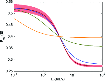
Figure 1.— The survival probability electron neutrinos $P_{ee}(E,\phi)$ and $\langle P_{ee}(E)\rangle$ in a 3+1 neutrino flavor oscillation model in which neutrino couple to the light dark matter field $\phi$ with fixed value of $m_{\phi}$ and $\epsilon_{\phi}$ (see main text). The figure shows $\langle P_{ee}(E)\rangle$ (with $\epsilon_{\phi}\approx 0\%$) for the following LDM models with $G_{\phi}/m_{\phi}$ ratios: $10^{29}\;{\rm G_{\rm F}\,eV^{-1}}$ (blue curve), $10^{30}\;{\rm G_{\rm F}\,eV^{-1}}$ (green curve), $10^{31}\;{\rm G_{\rm F}\,eV^{-1}}$ (orange curve). The figure also shows a model with $G_{\phi}\approx 0$ (red curve) and an ensemble of $P_{ee}(E,\phi)$ corresponding to different time-varying mass-square differences and angles for $\epsilon_{\phi}=1.5\%$ (pink band). See main text for details.

In the standard three-neutrino flavor model, the matter potential ${\cal V}$ takes into account the interaction of active neutrinos ($\nu_{e},\nu_{\mu},\nu_{\tau}$) with the ordinary fermions of the solar plasma, for which the ${\cal V}=\mathrm{{diag}}\{V_{cc}+V_{\rm nc},V_{\rm nc},V_{\rm nc}\}$ where $V_{\rm cc}$ corresponds to the weak charged current ($\rm cc$) that takes into account the forward scattering of $\nu_{e}$ with electrons, and $V_{\rm nc}$ is the weak neutral current ($\rm nc$) that corresponds to the scattering of the active neutrinos with the ordinary fermions of the solar plasma (e.g., Xing, 2020). $V_{\rm nc}$ can be expressed as $V_{\rm nc}=V^{e}_{\rm nc}+V^{p}_{\rm nc}+V^{n}_{\rm nc}$ where $V^{j}_{\rm nc}$ with $j=$ $e$, $p$, $n$ are the contributions coming from electrons, protons, and neutrons, respectively. However due to the electrical neutrality of the solar plasma, the contribution of $V^{e}_{\rm nc}$ and $V^{p}_{\rm nc}$ canceled out such that $V_{\rm nc}=V^{n}_{\rm nc}$. Accordingly, $V_{\rm cc}=\sqrt{2}G_{\rm F}\;n_{e}(r)$ and $V_{\rm nc}=V^{n}_{\rm nc}=G_{\rm F}/\sqrt{2}\;n_{n}(r)$. Here $G_{\rm F}$ is the Fermi constant and $n_{e}(r)$ and $n_{n}(r)$ are the number density of electrons and neutrons inside the Sun. Nevertheless, since $V_{\rm nc}$ is an universal term for all active neutrino flavors, and as such does not change the flavor oscillations pattern, conveniently we write ${\cal V}=\mathrm{{diag}}\{V_{\rm cc}+0,0,0\}$. Now, the inclusion of sterile neutrinos in the neutrino flavor model alters ${\cal V}$ (from Equation 8) by incorporating a new degree of freedom, as a consequence ${\cal V}=\mathrm{{diag}}\{V_{\rm cc}+V_{\rm nc},V_{\rm nc},V_{\rm nc},0\}$ (e.g., Giunti and Li, 2009; Maltoni and Smirnov, 2016; Xing, 2020).

Finally, in our 3+1 neutrino flavor model, we include the interaction of active and sterile neutrinos with the dark matter field $\phi$ by means of an intermediate heavy boson $I$. These interactions result from the forward scattering of these neutrinos through the LDM field $\phi$, thus ${\cal V}=\mathrm{{diag}}\{V_{\rm cc}+V_{\rm nc}+V_{\nu_{e}\phi},V_{\rm nc}+V_{\nu_{\mu}\phi},V_{\rm nc}+V_{\nu_{\tau}\phi},V_{\rm nc}+V_{\nu_{s}\phi}\}$, where $V_{\nu_{i}\phi}$ (with $\nu_{i}=\nu_{e},\nu_{\mu},\nu_{\tau},\nu_{s}$) relates to the neutrino $\nu_{i}$. This ${\cal V}$ corresponds to a generalization of the Wolfenstein potentials found in the literature, for which most neutrino flavor models only take into account the scattering of the sterile neutrinos on heavy dark matter (Capozzi et al., 2017; Lopes , 2018a; Lopes and Silk, 2019).

In our model, we opt to assume that all active neutrinos experience the same interaction with the LDM field $\phi$, such that their dark matter potentials are the same, such that $V_{\nu_{j}\phi}=V_{\nu_{a}\phi}$ (with $j=e,\mu,\tau$), it follows ${\cal V}=\mathrm{{diag}}\{V_{\rm cc}+V_{\rm nc}+V_{\nu_{a}\phi},V_{\rm nc}+V_{\nu_{a}\phi},V_{\rm nc}+V_{\nu_{a}\phi},V_{\rm nc}+V_{\nu_{s}\phi}\}$. Now, if we subtract the common term $V_{\rm nc}+V_{\nu_{a}\phi}$ to the diagonal matrix ${\cal V}$, the latter takes the simple form: ${\cal V}=\mathrm{{diag}}\{V_{\rm cc},0,0,V_{\nu_{s}\phi}-V_{\nu_{a}\phi}-V_{\rm nc}\}$.

The potential $V_{\nu_{i}\phi}$ (with $i=a,s$) is given by $V_{\nu_{i}\phi}=G_{\nu_{i}\phi}n_{\phi}$ where $G_{\nu_{i}\phi}$ is the equivalent of the Fermi constant and $n_{\phi}$ is the distribution of dark matter inside the Sun (Smirnov and Xu, 2019). Equally, $V_{\nu_{i}\phi}$ relates directly with the local density of dark matter $\rho^{\odot}_{\rm DM}$ by the expression: $V_{\nu_{s}\phi}=\left(G_{\nu_{s}\phi}/m_{\phi}\right)\left(\rho^{\odot}_{\rm DM}\Omega_{\phi}/\Omega_{\rm DM}\right)$, where we assume the ratio $G_{\nu_{s}\phi}/m_{\phi}$ is a free parameter of the LDM model. The generalized Fermi constant is defined as $G_{\nu_{i}\phi}=g_{\nu_{i}}g_{\phi}/m_{I}^{2}$ where $g_{\nu_{i}}$ represents the coupling constant of the corresponding neutrino $\nu_{i}$, and $m_{I}$ is the mass of the intermediate boson $I$ (Miranda et al., 2015). This expression for the potential $V_{\nu_{i}\phi}$ is valid since we assume that $m_{I}^{-1}\ll R_{\odot}$ where $R_{\odot}$ is the solar radius (Smirnov and Xu, 2019). In general, we could expect that the contribution of $\phi(t)$ to $V_{\nu_{i}\phi}$ could lead to a time-dependent relation, however, as discussed previously (in section 2.1) and mentioned for the first time by Khmelnitsky and Rubakov (2014), this is because the oscillatory component on the local density relates with $v_{\phi}^{2}$. This term is minimal, and therefore we neglected it.

In this preliminary study, without loss of generality, we choose to simplify ${\cal V}$ further: since the term $V_{\nu_{s}\phi}-V_{\nu_{a}\phi}-V_{\rm nc}$ has two Wolfenstein potentials ( $V_{\nu_{a}\phi}$ and $V_{\nu_{s}\phi}$) that effectively correspond to two new degrees of freedom, both of these have an identical impact on the neutrino flavor oscillation model. We choose to simplify the model by assuming that $V_{\nu_{a}\phi}$ is much smaller than $V_{\rm nc}$. Consequently, ${\cal V}$ takes the simplified form: ${\cal V}\approx\mathrm{{diag}}\{V_{\rm cc},0,0,V_{\nu_{s}\phi}-V_{\rm nc}\}$. For reference, we note that in the Sun’s core $V_{\rm nc}$ is always smaller than $V_{\rm cc}$, once $n_{e}$ is more than twice as lager as $n_{n}$ (e.g. Lopes, 2018b). This potential is identical to others found in the literature, for instance in Capozzi et al. (2017) and Lopes (2018a). Therefore, the matter potential $V_{\nu_{s}\phi}$ reads $V_{\nu_{s}\phi}=G_{\nu_{s}\phi}n_{\phi}$ where for convenience of analysis, we choose to define the generalized Fermi constant as $G_{\nu_{s}\phi}=4\sqrt{2}G_{\phi}G_{\rm F}$ where $G_{\phi}$ is our free parameter. Since these dark matter particles have a mass much smaller than $4\;{\rm GeV}$, the solar plasma conditions do not allow the accretion of dark matter by the Sun (e.g., Lopes and Lopes, 2019), therefore we will assume that the distribution of dark matter inside the star is equal to the value measured for the solar neighborhood $n_{\phi}$ (see section 2.1).

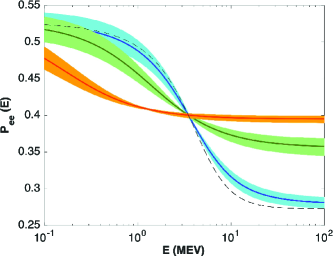
Figure 2.— The survival probability electron neutrinos $P_{ee}(E,\phi)$ and the corresponding $\langle P_{ee}(E)\rangle$ for some of the models shown in figure 1 for which $\epsilon_{\phi}=1.5\%$ : $G_{\phi}=10^{20}\;G_{\rm F}$ (blue band and dark blue curve), $G_{\phi}=10^{21}\;G_{\rm F}$ (green band and dark green curve) and $G_{\phi}=10^{22}\;G_{\rm F}$ (orange band and dark red curve). The figure also shows $\langle P_{ee}(E)\rangle$ for the 3+1 model with no time dependence ($G_{\chi}\approx 0$) and $\epsilon_{\phi}\approx 0$) as a thin dashed black curve. The latter curve corresponds to the red curve in figure 1.

3.2. Neutrino Flavor Oscillation Model and the Survival Probability of Electron Neutrinos

If we adopt as reference the current experimental set of parameters for the active neutrinos (e.g., Esteban et al., 2019), the propagation neutrinos in the solar interior are completely adiabatic. The same is valid for the 3+1 neutrino flavor oscillation model coupled to an LDM field $\phi$ considered in this study. Conveniently, the propagation of neutrinos away from resonances is well represented by a two neutrino flavor oscillation model. The motivation for such approximation can be found in Lopes (2018b) and references therein. In such a case, the electron neutrino flavor oscillation is dominated by the $(\nu_{1},\nu_{2})$ mass eigenstates and is only slightly affected by the decoupled $(\nu_{3},\nu_{4})$ eigenstates, since the associated mixing angles for the latter pair are very small (Kuo and Pantaleone, 1986). Moreover, $\nu_{3}$ and $\nu_{4}$ evolve independent of each other and are completely independent of the doublet $(\nu_{1},\nu_{2})$. In this limit, as proposed by several authors (e.g, Palazzo, 2011; Blennow and Smirnov, 2013), the split of the 3+1 neutrino flavor model into a dominant two neutrino flavor model ($\nu_{e},\nu_{\mu}$) with additional corrections for $\nu_{\tau}$ and $\nu_{s}$ significantly simplified the calculation and allowed us to obtain an analytical solution (e.g., Kuo and Pantaleone, 1989).

Among the many expressions available in the literature to compute the survival probability of electron neutrinos $P_{e}$ (e.g., Lunardini and Smirnov, 2000; Miranda et al., 2015) in a 3+1 neutrino flavor model developed in the approximate scenario of a two-flavor neutrino model (e.g., Kuo and Pantaleone, 1989), we opted to choose the expression obtained by Capozzi et al. (2017) for the case in which $V_{\rm cc}E/\Delta m_{31}^{2}\ll 1$ (and $s_{34}=0$) which has a better numerical accuracy than others. In that case the survival probability of electron neutrinos, i.e., $P_{e}$ $[\equiv P(\nu_{e}\rightarrow\nu_{e}]]$, reads

$$P_{ee}(E,\phi)=s_{13}^{4}+c_{13}^{4}c_{24}^{4}c_{14}^{4}+a_{m}+b_{m},$$ (9)

where $c_{ij}=\cos{\theta_{ij}}$ and $s_{ij}=\sin{\theta_{ij}}$. The functions $a_{m}$ and $b_{m}$ are dependent on the internal structure of the Sun and are given by the expressions:

$$a_{m}=C_{1}(s_{m}c_{14}-c_{m}s_{14}s_{24})^{2}$$ (10)

and

$$b_{m}=C_{2}(c_{m}c_{14}+s_{m}s_{14}s_{24})^{2}$$ (11)

where $c_{m}=\cos{\theta_{m}}$, $s_{m}=\sin{\theta_{m}}$, $C_{1}=c_{13}^{4}(c_{14}s_{12}-c_{12}s_{14}s_{24})^{2}$ and $C_{2}=c_{13}^{4}(c_{12}c_{14}+s_{12}s_{14}s_{24})^{2}$. The angle $\theta_{m}$ is obtained for the present-day Sun (i.e., the standard solar model, see details of this model in Lopes and Silk, 2013) using the expression (Capozzi et al., 2017): $\cos{(2\theta_{m})}={\cal M}_{x}({\cal M}_{y}^{2}+{\cal M}_{x}^{2})^{-1/2},$ where ${\cal M}_{x}\equiv\cos{(2\theta_{12})}-\eta_{\nu}V_{x}$ and ${\cal M}_{y}\equiv|\sin{(2\theta_{12})}+\eta_{\nu}V_{y}|$. $\eta_{\nu}$ is the ratio of the energy of the neutrino $E$ in relation to $\Delta m^{2}_{21}$ given by $\eta_{\nu}(E)=4E/\Delta m_{21}^{2}$. The functions $V_{x}$ and $V_{y}$ are given by

$$V_{x}=\frac{1}{2}\left[V_{\rm cc}c^{2}_{13}(c^{2}_{14}-s_{14}^{2}s_{24}^{2})+V_{s}(s_{14}^{2}-c_{14}^{2}s_{24}^{2})\right],$$ (12)

$$V_{y}=(V_{s}-V_{\rm cc}c_{13}^{2})c_{14}s_{14}s_{24}$$ (13)

and

$$V_{s}=V_{\nu_{s}\phi}-V_{\rm nc}.$$ (14)

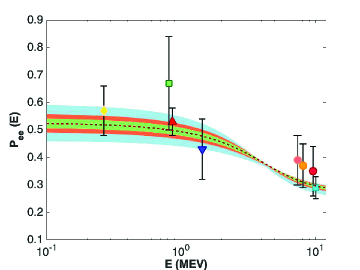
Figure 3.— The survival probability of the electron neutrinos for several solar nuclear reactions: $pp$ (yellow diamond), ${}^{7}Be$ (green square), ⁷Be (red upward triangle), $pep$ (blue downward triangle) and ⁸B HER (salmon circle), ⁸B HER-I (orange circle), ${}^{8}B$ HER-II (magenta circle) and ${}^{8}B$ (cyan square). The diamond, triangle, and circles points use data from the Borexino (Borexino Collaboration et al. , 2020; Agostini et al., 2019; Borexino Collaboration et al., 2018; Bellini et al., 2010) and the two square data points correspond to data obtained from SNO (Aharmim et al., 2013) and Super-Kamiokande (Abe et al., 2016; Cravens et al., 2008) detectors. Each color band corresponds to an ensemble of $P_{ee}(E,\phi)$ (Equation 9) in a 3+1 neutrino model with $G_{\phi}\approx 0$ and $\epsilon_{\phi}\approx 0$ (dashed curve), 1.5% (green), 3.0% (orange) and 6.0% (light blue). These survival probabilities are computed using an high-Z SSM (see the main text) and the experimental values from the different neutrino experiments.

3.3. Light Dark Matter Impact on Solar Neutrinos

The survival probability of electron neutrinos (Equation 9) is a time-dependent function through equations (6), (7) and (3). Conveniently we define an effective oscillation probability $\langle P_{ee}(E)\rangle$ that corresponds to an ensemble average of all the $P_{ee,}(E,\phi)$ (Equation 9), as such

$$\langle P_{ee}(E)\rangle=\int_{0}^{\tau_{\phi}}P_{ee}(E,\phi)\frac{dt}{\tau_{\phi}},$$ (15)

where $\tau_{\phi}=2\pi/m_{\phi}$ is the period of the LDM field $\phi(t)$.

The ability of a solar neutrino detector to measure the impact of the time-dependent LDM field $\phi(t)$ on the survival probability $P_{ee}(E,\phi)$ (Equation 9) depends on three characteristic time scales: the neutrino flight time $\tau_{\nu}$, the time between two consecutive neutrino detections $\tau_{ev}$, and the total run time of the experiment $\tau_{ex}$. The neutrino flight time is proportional to the Earth-Sun distance $d_{\earth}$ such that $\tau_{\nu}=d_{\earth}/c\approx 8.2\;{\rm min}$ where $c$ is the speed of light. The number of events measured by a detector varies strongly from one to another.

The next generation of experiments will have $\tau_{ev}$ much larger than the pioneer Homestake experiment that only detects a few events per year (Bahcall and Davis, 1976). The forthcoming Jiangmen Underground Neutrino Observatory (JUNO; Adam et al., 2015) experiment expects to measure a few tens of neutrinos per day (for instance 200 events per day or $\tau_{ev}\approx{\rm 7\;min}$). The total experimental run time for most solar neutrino detectors is of the order of a few decades (for instance $\tau_{ex}\approx{\rm 10\;yr}$), and future experiments will also have significant running times. Hence for all models considered in this study, we assume that solar neutrino detectors will run for long periods and will collect a large number of events, therefore we assume that $\tau_{ev}$ and $\tau_{ex}$ have sufficient small and large values, respectively.

In such conditions, the solar neutrino spectra time modulation by $\phi(t)$ depends on the period $\tau_{\phi}$ of the LDM field in comparison to the flight time of solar neutrinos $\tau_{\nu}$. Since these neutrinos have a $\tau_{\nu}\approx 8.2\;{\rm min}$, it is possible to find the value of $m_{\phi}$ for which $\tau_{\nu}=\tau_{\phi}$ which occurs for $m_{\phi,c}=8.3\;10^{-18}\;{\rm eV}$. Accordingly, we can define two regimes for the time modulation of survival probability of electron neutrinos :

1. For $\tau_{\phi}\geq\tau_{\nu}$ (low-frequency regime or low LDM mass), the time modulation of $P_{ee}(E,\phi)$ occurs when the period of $\phi(t)$ is larger than $\tau_{\nu}$. In this case a temporal variation of the neutrino signal may be observed. This corresponds to a LDM field with a mass such that $m_{\phi}\leq m_{\phi,c}$. Therefore, the LDM field can induce an observable time variation in neutrino oscillation measurements as periodicity in the solar neutrino fluxes (Berlin, 2016). Obviously, if $\tau_{\phi}$ becomes very large, the modulation of $P_{ee}(E,\phi)$ becomes indistinguishable from the standard scenario (undistorted case), since the running time of the experiment is not sufficient to observe this phenomena. Nevertheless, in our study, the LDM field has always an $m_{\phi}\geq 10^{-23}\;{\rm eV}$ or a period $\tau_{\phi}\geq 13\;{\rm yr}$. Therefore, it is always possible to probe such a model with current experimental running times.

2. For $\tau_{\phi}\leq\tau_{\nu}$ (high-frequency regime or high LDM mass), the change of $P_{ee}(E,\phi)$ due to $\phi(t)$ is too fast to be observed as a modulating signal like in the previous case. This regime occurs for LDM fields with a mass such that $m_{\phi}\geq m_{\phi,c}$. Nevertheless, the time average of the ensemble of oscillation probability $P_{ee}(E,\phi)$ can be distorted in such a regime, hence the effect can be detected as $\langle P_{ee}(E)\rangle$ which will deviate from the standard scenario (Krnjaic et al., 2018). The net effect of averaging over time induces a shift in the observed values of $P_{ee}(E,\phi)$ relative to its undistorted value.

Therefore, we can expect to study both regimes in a quite reasonable range of LDM masses using data from the present and future solar neutrino experiments. In fact, some of the current solar neutrino detectors have already large statistics and high event rates that we can use to look for time modulations in solar neutrinos. Some of these neutrino collaborations have already searched for regular phenomena with periods varying from 10 minutes to 10 yr (e.g., Yoo et al., 2003; Aharmim et al., 2010).

In this work, we will study models that will fall in these two regimes of time modulation. Therefore to satisfy the conditions mentioned above, we decided to analyze the impact of the LDM field in solar neutrino fluxes for $\phi(t)$ with a period $\tau_{\phi}$ varying from $4\;\mu{\rm s}$ to $13\;{\rm yr}$ or equivalently with a $m_{\phi}$ varying from $10^{-9}\;{\rm eV}$ to $10^{-23}\;{\rm eV}$, which is a range possible to be scanned by future detectors like Deep Underground Neutrino Experiment (DUNE Collaboration et al., 2015) and JUNO (An et al., 2016).

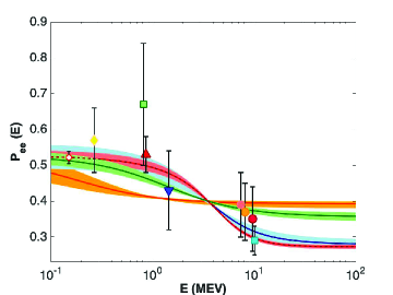
Figure 4.— The survival probability of the electron neutrinos for several LDM models (see the main text and caption of figure 3 and 2 for details). The LDM models are identical to the ones presented in Figure 2, with the following changes: (i) $G_{\phi}=0$ and $\epsilon_{\phi}=1.5\%$ (red band); (ii) $G_{\phi}=10^{20}G_{\rm F}$ and $\epsilon_{\phi}=3.0\%$ (light-blue band); (iii) $G_{\phi}=10^{21}G_{\rm F}$ and $\epsilon_{\phi}=1.5\%$ (green band); (iv) $G_{\phi}=10^{22}G_{\rm F}$ and $\epsilon_{\phi}=3.0\%$ (orange band). The data points correspond to the same ones displayed in figure 3. However, the data with the lowest energy corresponds to the expected precision to be attained by the Darwin experiment in measuring $P_{ee}\pm\Delta P_{ee}$, for which $\Delta P_{ee}$ could be as low as $\Delta P_{ee}=0.017$ (Aalbers et al., 2020). The continuous dashed curve corresponds to a 3+1 neutrino model with $G_{\phi}\approx 0$ and $\epsilon=0\%$.

4. Light Dark Matter Impact on Electron Neutrino Spectra

Inside the Sun, the flux variation of neutrinos with different flavors due to matter (including LDM) is strongly dependent of the local distributions of electrons and neutrons, but also on the population of dark matter particles in the solar neighbourhood. This new flavor mechanism (sterile neutrinos and LDM field $\phi$) affects all electron neutrinos produced in the Sun’s core. A detailed discussion about the neutrino sources inside the Sun, and their specific solar properties, can be found in Lopes (2013, 2017). The average survival probability of electron neutrinos for each nuclear reaction in the solar interior, i.e., $P_{e,i}(E,\phi)$ is computed by

$$P_{ee,i}(E,\phi)=C_{i}\int_{0}^{R_{\odot}}P_{e}(E,\phi,r)S_{i}(r)4\pi\rho(r)r^{2}dr,$$ (16)

where $C_{i}$ $\left(=\left[\int_{0}^{R_{\odot}}S_{i}(r)4\pi\rho(r)r^{2}\;dr\right]^{-1}\right)$ is a normalization constant and $S_{i}(r)$ is the electron neutrino emission function for the $i$ solar nuclear reaction. $i$ corresponds to the following solar neutrino sources (from the PP chain and CNO cycle nuclear reactions): $pp$, $pep$, ⁸B, ⁷Be, ¹³N, ¹⁵O and ¹⁷F.

Moreover, since the survival probabilities $P_{ee,i}(E,\phi)$ (Equation 16) are time dependent through $\phi$, these quantities also vary with time. Therefore, the oscillation probability $\langle P_{ee}(E)\rangle$ (Equation 15) is generalized for each specific nuclear reaction $i$:

$$\langle P_{ee,i}(E)\rangle=\int_{0}^{\tau_{\phi}}P_{e,i}(E,\phi)\frac{dt}{\tau_{\phi}}.$$ (17)

The LDM field $\phi$ can lead to different temporal imprints on the neutrino oscillation measurements. The specific impact depends on the mass of the LDM particle. In the following, we compute the spectra of neutrinos from any specific nuclear reaction that we know to be essentially independent of the properties surrounding solar plasma. Since in the 3+1 neutrino flavor model new processes exist to change the survival probability of electron neutrinos, this will modify the solar neutrino spectra measured on Earth. These new processes will alter the conversion rates of $\nu_{e}$ to other flavors ($\nu_{\mu}$, $\nu_{\tau}$ and $\nu_{s}$) and vice versa. Accordingly, the electron neutrino spectrum of the nuclear reaction $i$ inside the core is defined as $\Phi_{i}$, and $\Phi_{i\odot}$ is the electron neutrino spectrum arriving on Earth (Lopes, 2018b) such that:

$$\Phi_{i,\odot}(E)=P_{ee,i}(E,\phi)\Phi_{i}(E)$$ (18)

where $P_{ee,i}(E)$ is the average survival probability of electron neutrinos for reactions in the solar interior as given by equation 16. Equally if we take the time average of equation 18, we obtain the following averaged spectrum for each nuclear reaction $i$:

$$\Phi_{i,\odot}(E)=\langle P_{ee,i}(E)\rangle\Phi_{i}(E),$$ (19)

where $\langle P_{ee,i}(E)\rangle$ is the average survival probability of electron neutrinos as given by equation 17.

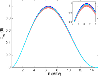
Figure 5.— The ${}^{8}B$ solar electron neutrino spectra measured on Earth detectors. The blue curve corresponds to the standard (undistorted) neutrino spectra, the cyan curve to the averaged (distorted) electron spectra, and the red band corresponds to the ensemble of spectra related with the time-dependent flavor parameters. This LDM model has a $G_{\phi}\approx 0$ and an $\epsilon_{\phi}=3.0\%$. In the calculation of the ⁸B spectrum we use a high-Z SSM (see the main text).

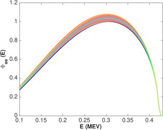
Figure 6.— The $pp$ solar electron neutrino spectra measured on Earth detectors. The LDM model and color scheme is the same one as in Figure 5. The error bar curves (yellow curves) on the averaged (distorted) electron spectra (cyan curve) corresponds to the expected precision to be attained by the Darwin experiment (Aalbers et al., 2020). See Figure 4 and main the text.

5. The Sun: Light Dark Matter and Sterile Neutrinos

Here, we will study the impact of the theoretical model presented in the previous sections, specifically we compute the survival probability of electron neutrinos (as given by equations (9), (15), (16) and (17)) in the case of a standard solar model with low-Z (e.g., Lopes and Silk, 2013; Capelo and Lopes, 2020).

In the parameterization for the 3+1 neutrino flavor oscillation model, we opt to adopt the recent values obtained in the data analysis of the standard three-neutrino flavor oscillation model obtained by de Salas et al. (2020), and for the sterile neutrino additional fiducial parameters we used the values obtained by Gariazzo et al. (2015). Accordingly, for a parameterisation with a normal ordering of neutrino masses, the mass-square difference and the mixing angles have the following values: $\Delta m^{2}_{21}=7.50^{+0.22}_{-0.20}\times 10^{-5}{\rm eV^{2}}$, $\sin^{2}{\theta_{12}}=0.318\pm 0.016$, and $\sin^{2}{\theta_{13}}=0.02250^{+0.00055}_{-0.00078}$. Although, $\Delta m^{2}_{31}=2.56^{+0.0003}_{-0.0004}\times 10^{-3}{\rm eV^{2}}$ and $\sin^{2}{\theta_{23}}=0.56^{+0.016}_{-0.022}$, we mention them here for reference (de Salas et al., 2020). These new parameters are consistent with previous estimations (Esteban et al., 2019; Gonzalez-Garcia et al., 2016). For the sterile neutrino, we choose the following fiducial values for the mass-square difference and mixing angles  (Gariazzo et al., 2015, 2016; Capozzi et al., 2017): $\Delta m^{2}_{41}=1.6\ {\rm eV^{2}}$, $\sin^{2}{\theta_{14}}=0.027$, $\sin^{2}{\theta_{42}}=0.014$ and the other mixing angle for the sterile neutrinos are fixed to zero. Moreover, we assume that all phases ($\delta_{13,14,34}$) and other angles related to the sterile neutrino are equal to zero.

The present-day internal structure of the Sun corresponds to an up-to-date standard solar model (SSM) that has a better agreement with neutrino fluxes and helioseismic data sets. This solar model was obtained from a one-dimensional stellar evolution code allowed to evolve in time until the present-day solar age, $4.57$ Gyr, having been calibrated to the values of luminosity and effective temperature of the present Sun, of $3.8418\times 10^{33}$ erg s^-1 and $5777$ K, respectively, as well as the observed abundance ratio at the Sun’s surface: ($Z_{\text{s}}/X_{\text{s}}$)${}_{\odot}=0.0181$, where $Z_{s}$ and $X_{s}$ are the metal and hydrogen abundances at the surface of the star (Turck-Chieze and Lopes, 1993; Bahcall et al., 1995, 2006). This stellar model was computed with the release version 12115 of the stellar evolution code MESA (Paxton et al., 2011, 2019). The details about the physics of this standard solar model in which we use the AGSS09 (low-Z) solar abundances (Asplund et al., 2009) are described in Lopes and Silk (2013) and Capelo and Lopes (2020).

Figures 1 and 2 show the impact of the time-dependent mass-square difference (Equation 6) and mixing angles (Equation 7) on the averaged electron survival probability $\langle P_{ee}(E)\rangle$ (Equation 15) for which the LDM field $\phi$ has a fixed amplitude (Equation 5): $\epsilon_{\phi}=0$ or $\epsilon_{\phi}=1.5\%$. We also show LDM models for which the sterile neutrino couples to $\phi$ with strength $G_{\phi}$.

The overall shape of the curve $\langle P_{ee}(E)\rangle$ depends on $G_{\phi}$ times $n_{\phi}$ in the potential $V_{\nu_{s}\phi}$ or the ratio $G_{\phi}/m_{\phi}$ as previously mentioned. For instance, in a LDM model in which we fix $m_{\phi}=10^{-9}\;{\rm eV}$ (or $n_{\phi}$), an increase of $G_{\phi}$ from $10^{20}$ to $10^{22}\;G_{\rm F}$ leads $\langle P_{ee}(E)\rangle$ to vary significantly, as shown in Figure 1. As expected this change in $\langle P_{ee}(E)\rangle$ is more pronounced for high energy neutrinos where the MSW effect is more significant. If we choose higher values of $m_{\phi}$ the results will somehow be similar (see Figure 1).

Evidently, for an LDM model in which $m_{\phi}$ decreases by a certain amount ($n_{\phi}=\rho_{\phi}/m_{\phi}$), the constancy of $G_{\phi}/m_{\phi}$ in $V_{\nu_{s}\phi}$ implies that $G_{\phi}$ can increase by the same order of magnitude to obtain the same MSW effect on the $\langle P_{ee}(E)\rangle$ curve (see Figure 1). For instance, an LDM model with $m_{\phi}=10^{-23}\;{\rm eV}$ and $G_{\phi}=10^{7}G_{\rm F}$ will have $\langle P_{ee}(E)\rangle$ identical to an LDM model with $m_{\phi}=10^{-9}\;{\rm eV}$ and $G_{\phi}=10^{21}G_{\rm F}$ , since in both LDM models we have the same ratio: $G_{\phi}/m_{\phi}\approx 10^{30}$. The same argument explains the reason why the coupling constant between sterile neutrinos and more massive dark matter particles is much smaller in those models than in the present study. For instance, this is the case for particles captured from the dark matter halo by the Sun. Since over time, the star accreted a significant amount of dark matter (e.g., Lopes , 2018a), for these models $G_{\phi}$ is significantly smaller than the value found for the present study.

The most important feature of such a class of LDM models is the time dependence of the dark matter field $\phi(t)$ and its imprint in the flavor oscillation parameters’ mass-square differences (Equation 6) and mixing angles (Equation 7). As predicted by equation 9, there are many $P_{ee}(E,\phi)$ with near similar behavior. Figure 1 shows an ensemble of time-dependent $P_{ee}(E,\phi)$ as a pink band. The difference between curves relates to the dependence of the oscillation parameters on time. In this LDM model it is assumed there is a very negligible interaction between sterile neutrinos and $\phi$ (for which $G_{\phi}\approx 0$). The figure also shows $\langle P_{ee}(E)\rangle$ (red curve) the time-averaged of the ensemble of $P_{ee}(E,\phi)$ curves that we compute using equation 15.

Although there are several parameters that contribute for the time variability of $P_{ee}(E,\phi)$ (Equation 9), the main contributions come from $\theta_{21}$ and $\theta_{13}$. The variability related $\theta_{24}$ is relevant for the high energies. We notice that the contributions coming from $\Delta m^{2}_{21}$ and $\theta_{32}$ are much smaller than all the parameters mentioned above. The amplitude of the $P_{ee}(E,\phi)$ pink band is defined by the value of $\epsilon_{\phi}$ for which we adopt the fiducial value of $\epsilon_{\phi}=1.5\%$. It is worth pointing out that the $P_{ee}(E,\phi)$ band is much larger for low-energy than for higher-energy values. Moreover, the averaged value of this ensemble given by $\langle P_{ee}(E)\rangle$ is identical to $\langle P_{ee}(E)\rangle$ with $\epsilon_{\phi}\approx 0$. Figure 2 shows the variability of $P_{ee}(E,\phi)$ for a LDM with different $G_{\phi}$ values. These results are identical to the model in figure 1. Nevertheless, the LDM model with the largest $G_{\phi}$ has (an orange) band with a smaller amplitude around $\langle P_{ee}(E)\rangle$. Once again, the band thickness decreases for neutrinos with higher energy for all these models.

Figures 3 and 4 compare our predictions with current solar neutrino data (e.g., Aalbers et al., 2020). These figures show that LDM models with relatively low values of $\epsilon_{\phi}$ and $G_{\phi}$ are compatible overall with current solar neutrino data coming from Borexino, Super-Kamiokande, and SNO. Clearly, this analysis has also shown that the precision of our current solar neutrino experiments is not able to distinguish between some of these LDM models. Nevertheless, it is already possible to put some constraints on these LDM models. For instance, we found that LDM models with $G_{\phi}\approx 0$ must have a $\epsilon_{\phi}$ smaller than $3\%$ to be consistent with all data, including $pp$ measurements of the Borexino detector (Borexino Collaboration et al. , 2020) (see Figure 3); and any LDM models must have a ratio $G_{\phi}/m_{\phi}$ smaller than $10^{30}$, otherwise they become inconsistent with $pp$ and ⁷Be measurements for several solar detectors (Borexino Collaboration et al. , 2020; Agostini et al., 2019; Borexino Collaboration et al., 2018; Bellini et al., 2010) (see figure 4). Figure 4 shows a LDM model with a $m_{\phi}=10^{-9}\;{\rm eV}$ and $G_{\phi}=10^{22}\;G_{\rm F}$ with a ratio $G_{\phi}/m_{\phi}$ of the order of $10^{31}\;G_{\rm F}$ (see Figure 4); This ratio is one order of magnitude larger than the critical $G_{\phi}/m_{\phi}$ value of $10^{30}$ discussed in the previous section. Figure 4 also shows that the variability related with time dependence on $P_{ee}(E,\phi)$ decreases for large values of $G_{\phi}$.

There is another important effect that also contributes to the time variability of $P_{ee}(E,\phi)$. The PP chain and CNO cycle, nuclear reactions occur at different distances from the center of the Sun and each nuclear reaction emits neutrinos in a well-defined energy range. As a consequence, the electron neutrinos produced in each specific nuclear reaction will be affected differently by the MSW effect. As such, this effect will also contribute to the overall variability of electron neutrinos $P_{ee,i}(E,\phi)$ (see Equation 16) and their time-averaged $\langle P_{ee,i}(E,\phi)\rangle$ (see Equation 17).

The time-dependent electron neutrino survival probability will have a significant impact on the neutrino spectra of the different nuclear reactions. Accordingly, figures 5 and 6 show the spectra correspond to two neutrino types: $pp$ and ${}^{8}B$ neutrinos. An essential difference between these two spectra relates to the thickness of the $\epsilon_{\phi}$ band for a fixed value since thickness decreases with neutrino energy. Therefore the $\epsilon_{\phi}$ band is more significant for a $pp$ spectrum than for a ${}^{8}B$ neutrino spectrum. This is an effect identical to the one discussed previously for the $P_{ee}(E,\phi)$ functions. Therefore, the measurement of solar neutrino fluxes and solar neutrino spectrum in the energy range below $0.2\;MeV$ will provide the strongest constraint for such a class of dark matter models. Figure 5 and 6 show the spectra of ⁸B and $pp$, if we assume the precision expected to be attained by the Darwin experiment (Aalbers et al., 2020). Figure 6 also shows the precision expected for the Darwin experiment.

6. Conclusion

This article focuses on the impact of LDM on solar neutrino fluxes, spectra, and survival probabilities of electron neutrinos, specifically a dark matter model made of two particles: a sterile neutrino and an LDM particle. In particular, we describe how the 3+1 neutrino flavor model is affected by this type of LDM particles, with an emphasis on how the LDM affects the Wolfenstein potentials. We also study how the dark matter models affect the survival probability functions of electron neutrinos related to the different nuclear reactions occurring in the solar interior, and we compute the spectra of two relevant solar neutrino sources: $pp$ and ${}^{8}B$ neutrino nuclear reactions.

By studying a large range of dark matter particle masses (from $10^{-9}$ to $10^{-23}\;{\rm eV}$) we found that depending on the mass of these LDM particles and the value of the generalized Fermi constant, the shape of electron neutrino survival probability and their spectra can vary with time. We establish that for LDM particles with low masses (low-frequency regime), the solar neutrino detectors can observe the electron neutrino survival probability changing with time. Conversely, for dark matter particles with higher masses (high-frequency regime), this impact can be determined by measuring the time-averaged electron neutrino survival probability.

It was possible to establish, using data of current solar neutrino measurements, that those models with a $G_{\phi}/m_{\phi}$ ratio smaller than $10^{30}\;G_{\rm F}eV^{-1}$ agree with current solar neutrino data from the Borexino, SNO and Super-Kamiokande detectors. We also found that for models with a near-zero constant, the time-variability amplitude must be smaller than 3%. Such a constraint is equivalent to the condition ${g_{\phi}\sqrt{2\rho^{\odot}_{\rm DM}}}/{(m_{\phi}m_{\nu})}\;\left({\Omega_{\phi}}/{\Omega_{\rm DM}}\right)^{1/2}\leq 0.03$.

Finally, we also found that the precision expected in the measurements to be made by the Darwin detector will allow us to put powerful constraints to this class of models.

References

- Aalbers et al. (2020) Aalbers, J., and 166 colleagues 2020, ”Solar Neutrino Detection Sensitivity in DARWIN via Electron Scattering”, arXiv e-prints, arXiv:2006.03114.
- Abe et al. (2016) Abe, K., and 169 colleagues 2016, ”Solar neutrino measurements in Super-Kamiokande-IV”, Phys. Rev. D, 94, 052010.
- Adam et al. (2015) Adam, T., and 396 colleagues 2015, ”JUNO Conceptual Design Report”, arXiv e-prints, arXiv:1508.07166.
- Agostini et al. (2019) Agostini, M., and 107 colleagues 2019, ”Simultaneous precision spectroscopy of p p , 7Be, and p e p solar neutrinos with Borexino Phase-II”, Phys. Rev. D, 100, 082004.
- Aharmim et al. (2010) Aharmim, B., and 124 colleagues 2010, ”Searches for High-frequency Variations in the 8B Solar Neutrino Flux at the Sudbury Neutrino Observatory”, ApJ, 710, 540-548.
- Aharmim et al. (2013) Aharmim, B., and 122 colleagues 2013, ”Combined analysis of all three phases of solar neutrino data from the Sudbury Neutrino Observatory”, Phys. Rev. C, 88, 025501.
- Aguilar et al. (2001) Aguilar, A., and 25 colleagues 2001, ”Evidence for neutrino oscillations from the observation of appearance in a beam”, Phys. Rev. D, 64, 112007.
- Arvanitaki et al. (2016) Arvanitaki, A., S. Dimopoulos, and K. Van Tilburg 2016, ”Sound of Dark Matter: Searching for Light Scalars with Resonant-Mass Detectors”, Phys. Rev. Lett., 116, 031102.
- Arvanitaki et al. (2018) Arvanitaki, A., P. W. Graham, J. M. Hogan, S. Rajendran, and K. Van Tilburg 2018, ”Search for light scalar dark matter with atomic gravitational wave detectors”, Phys. Rev. D, 97, 075020.
- Asplund et al. (2009) Asplund, M., N. Grevesse, A. J. Sauval, and P. Scott 2009, ”The Chemical Composition of the Sun”, ARA&A, 47, 481-522.
- An et al. (2016) An, F., and 227 colleagues 2016, ”Neutrino physics with JUNO”, Journal of Physics G Nuclear Physics, 43, 030401.
- Bahcall and Davis (1976) Bahcall, J. N. and R. Davis 1976, ”Solar Neutrinos: A Scientific Puzzle”, Science, 191, 264-267.
- Bahcall et al. (1995) Bahcall, J. N., M. H. Pinsonneault, and G. J. Wasserburg 1995, ”Solar models with helium and heavy-element diffusion”, Reviews of Modern Physics, 67, 781-808.
- Bahcall et al. (2006) Bahcall, J. N., A. M. Serenelli, and S. Basu 2006, ”10,000 Standard Solar Models: A Monte Carlo Simulation”, ApJS, 165, 400-431.
- Bellini et al. (2010) Bellini, G., and 86 colleagues 2010, ”Measurement of the solar B8 neutrino rate with a liquid scintillator target and 3 MeV energy threshold in the Borexino detector”, Phys. Rev. D, 82, 033006.
- Berlin (2016) Berlin, A. 2016, ”Neutrino Oscillations as a Probe of Light Scalar Dark Matter”, Phys. Rev. Lett., 117, 231801.
- Bezrukov et al. (2019) Bezrukov, F., A. Chudaykin, and D. Gorbunov 2019, ”Induced resonance makes light sterile neutrino dark matter cool”, Phys. Rev. D, 99, 083507.
- Bezrukov et al. (2020) Bezrukov, F., A. Chudaykin, and D. Gorbunov 2020, ”Scalar induced resonant sterile neutrino production in the early Universe”, Phys. Rev. D, 101, 103516.
- Blas et al. (2017) Blas, D., D. L. Nacir, and S. Sibiryakov 2017, ”Ultralight Dark Matter Resonates with Binary Pulsars”, Phys. Rev. Lett., 118, 261102.
- Blennow and Smirnov (2013) Blennow, M. and A. Y. Smirnov 2013, ”Neutrino Propagation in Matter”, arXiv e-prints, arXiv:1306.2903.
- Borexino Collaboration et al. (2020) Borexino Collaboration et al., Agostini, M., and 98 colleagues 2020, ”Improved measurement of 8B solar neutrinos with 1.5 kt .y of Borexino exposure”, Phys. Rev. D, 101, article id.062001.
- Borexino Collaboration et al. (2018) Borexino Collaboration, M. Agostini, and 108 colleagues 2018, ”Comprehensive measurement of pp-chain solar neutrinos”, Nature, 562, 505-510.
- Brdar et al. (2018) Brdar, V., J. Kopp, J. Liu, P. Prass, and X.-P. Wang 2018, ”Fuzzy dark matter and nonstandard neutrino interactions”, Phys. Rev. D, 97, 043001.
- Catena and Ullio (2010) Catena, R. and P. Ullio 2010, ”A novel determination of the local dark matter density”, Journal of Cosmology and Astroparticle Physics, 2010, 004.
- Capelo and Lopes (2020) Capelo, D. and I. Lopes 2020, ”The impact of composition choices on solar evolution: age, helio- and asteroseismology, and neutrinos”, MNRAS, 498, 1992-2000.
- Capozzi et al. (2017) Capozzi, F., I. M. Shoemaker, and L. Vecchi 2017, ”Solar neutrinos as a probe of dark matter-neutrino interactions”, Journal of Cosmology and Astroparticle Physics, 2017, 021.
- Cravens et al. (2008) Cravens, J. P., and 144 colleagues 2008, ”Solar neutrino measurements in Super-Kamiokande-II”, Phys. Rev. D, 78, 032002.
- Dasgupta and Kopp (2014) Dasgupta, B. and J. Kopp 2014, ”Cosmologically Safe eV-Scale Sterile Neutrinos and Improved Dark Matter Structure”, Phys. Rev. Lett., 112, 031803.
- de Gouvêa et al. (2020) de Gouvêa, A., M. Sen, W. Tangarife, and Y. Zhang 2020, ”Dodelson-Widrow Mechanism in the Presence of Self-Interacting Neutrinos”, Phys. Rev. Lett., 124, 081802.
- Dev et al. (2020) Dev, A., P. A. N. Machado, and P. Martínez-Miravé 2020, ”Signatures of Ultralight Dark Matter in Neutrino Oscillation Experiments”, arXiv e-prints, arXiv:2007.03590.
- de Salas et al. (2020) de Salas, P. F., D. V. Forero, S. Gariazzo, P. Martínez-Miravé, O. Mena, C. A. Ternes, M. Tórtola, and J. W. F. Valle 2020, ”2020 Global reassessment of the neutrino oscillation picture”, arXiv e-prints, arXiv:2006.11237.
- Diaz et al. (2019) Diaz, A., C. A. Argüelles, G. H. Collin, J. M. Conrad, and M. H. Shaevitz 2019, Where Are We With Light Sterile Neutrinos?, arXiv e-prints, arXiv:1906.00045.
- Ding and Feruglio (2020) Ding , G-J., F. Feruglio Testing Moduli and Flavon Dynamics with Neutrino Oscillations, arXiv e-prints, arXiv:2003.13448.
- Dodelson and Widrow (1994) Dodelson, S. and L. M. Widrow 1994, ”Sterile neutrinos as dark matter”, Phys. Rev. Lett., 72, 17-20.
- Dror et al. (2019) Dror, J. A., K. Harigaya, and V. Narayan 2019, ”Parametric resonance production of ultralight vector dark matter”, Phys. Rev. D, 99, 035036.
- DUNE Collaboration et al. (2015) DUNE Collaboration, R. Acciarri, and 804 colleagues 2015, ”Long-Baseline Neutrino Facility (LBNF) and Deep Underground Neutrino Experiment (DUNE) Conceptual Design Report Volume 2: The Physics Program for DUNE at LBNF”, arXiv e-prints, arXiv:1512.06148.
- Esteban et al. (2019) Esteban, I., M. C. Gonzalez-Garcia, A. Hernandez-Cabezudo, M. Maltoni, and T. Schwetz 2019, ”Global analysis of three-flavour neutrino oscillations: synergies and tensions in the determination of 23, CP, and the mass ordering”, Journal of High Energy Physics, 2019, 106.
- Farzan (2019) Farzan, Y. 2019, ”Ultra-light scalar saving the 3 + 1 neutrino scheme from the cosmological bounds”, Physics Letters B, 797, 134911.
- Graham et al. (2016) Graham, P. W., D. E. Kaplan, J. Mardon, S. Rajendran, and W. A. Terrano 2016, ”Dark matter direct detection with accelerometers”, Phys. Rev. D, 93, 075029.
- Gariazzo et al. (2016) Gariazzo, S., C. Giunti, M. Laveder, Y. F. Li, and E. M. Zavanin 2016, ”Light sterile neutrinos”, Journal of Physics G Nuclear Physics, 43, 033001.
- Gariazzo et al. (2015) Gariazzo, S., C. Giunti, M. Laveder, Y. F. Li, and E. M. Zavanin 2015, ”Light sterile neutrinos”, Journal of Physics G Nuclear Physics, 43, 033001.
- Gonzalez-Garcia et al. (2016) Gonzalez-Garcia, M. C., M. Maltoni, and T. Schwetz 2016, ”Global analyses of neutrino oscillation experiments”, Nuclear Physics B, 908, 199-217.
- Giunti and Li (2009) Giunti, C. and Y. F. Li 2009, ”Matter effects in active-sterile solar neutrino oscillations”, Phys. Rev. D, 80, 113007.
- Giunti et al. (2012) Giunti, C., M. Laveder, Y. F. Li, Q. Y. Liu, and H. W. Long 2012, ”Update of short-baseline electron neutrino and antineutrino disappearance”, Phys. Rev. D, 86, 113014.
- Giunti et al. (2013) Giunti, C., M. Laveder, Y. F. Li, and H. W. Long 2013, ”Short-baseline electron neutrino oscillation length after the Troitsk experiment”, Phys. Rev. D, 87, 013004.
- Hannestad et al. (2014) Hannestad, S., R. S. Hansen, and T. Tram 2014, ”How Self-Interactions can Reconcile Sterile Neutrinos with Cosmology”, Phys. Rev. Lett., 112, 031802.
- Hu et al. (2000) Hu, W., R. Barkana, and A. Gruzinov 2000, ”Fuzzy Cold Dark Matter: The Wave Properties of Ultralight Particles”, Phys. Rev. Lett., 85, 1158-1161.
- Hui et al. (2017) Hui, L., J. P. Ostriker, S. Tremaine, and E. Witten 2017, ”Ultralight scalars as cosmological dark matter”, Phys. Rev. D, 95, 043541.
- Khmelnitsky and Rubakov (2014) Khmelnitsky, A. and V. Rubakov 2014, ”Pulsar timing signal from ultralight scalar dark matter”, Journal of Cosmology and Astroparticle Physics, 2014, 019.
- Krnjaic et al. (2018) Krnjaic, G., P. A. N. Machado, and L. Necib 2018, ”Distorted neutrino oscillations from time varying cosmic fields”, Phys. Rev. D, 97, 075017.
- Kuo and Pantaleone (1986) Kuo, T. K. and J. Pantaleone 1986, ”Solar-neutrino problem and three-neutrino oscillations.”, Phys. Rev. Lett., 57, 1805-1808.
- Lopes (2013) Lopes, I. 2013, ”Probing the Sun’s inner core using solar neutrinos: A new diagnostic method”, Phys. Rev. D, 88, 045006.
- Lopes (2017) Lopes, I. 2017, ”New neutrino physics and the altered shapes of solar neutrino spectra”, Phys. Rev. D, 95, 015023.
- Lopes (2018a) Lopes, I. 2018, ”The Sterile-Active Neutrino Flavor Model: The Imprint of Dark Matter on the Electron Neutrino Spectra”, ApJ, 869, 112.
- Lopes (2018b) Lopes, I. 2018, ”The spectroscopy of solar sterile neutrinos”, European Physical Journal C, 78, 327.
- Lopes and Lopes (2019) Lopes, J. and I. Lopes 2019, ”Asymmetric Dark Matter Imprint on Low-mass Main-sequence Stars in the Milky Way Nuclear Star Cluster”, ApJ, 879, 50.
- Lopes and Silk (2019) Lopes, I. and J. Silk 2019, ”Dark matter imprint on 8B neutrino spectrum”, Phys. Rev. D, 99, 023008.
- Lopes and Silk (2014) Lopes, I. and J. Silk 2014, ”Helioseismology and Asteroseismology: Looking for Gravitational Waves in Acoustic Oscillations”, ApJ, 794, 32.
- Lopes and Turck-Chièze (2013) Lopes, I. and S. Turck-Chièze 2013, ”Solar Neutrino Physics Oscillations: Sensitivity to the Electronic Density in the Sun’s Core”, ApJ, 765, 14.
- Lopes and Silk (2013) Lopes, I. and J. Silk 2013, ”Planetary influence on the young Sun’s evolution: the solar neutrino probe”, MNRAS, 435, 2109-2115.
- Lunardini and Smirnov (2000) Lunardini, C. and A. Y. Smirnov 2000, ”The minimum width condition for neutrino conversion in matter”, Nuclear Physics B, 583, 260-290.
- Kuo and Pantaleone (1989) Kuo, T. K. and J. Pantaleone 1989, ”Neutrino oscillations in matter”, Reviews of Modern Physics, 61, 937-980.
- Kostensalo et al. (2019) Kostensalo, J., J. Suhonen, C. Giunti, and P. C. Srivastava 2019, ”The gallium anomaly revisited”, Physics Letters B, 795, 542-547.
- Kusenko (2009) Kusenko, A. 2009, ”Sterile neutrinos: The dark side of the light fermions”, Phys. Rep., 481, 1-28.
- Maltoni and Smirnov (2016) Maltoni, M. and A. Y. Smirnov 2016, ”Solar neutrinos and neutrino physics”, European Physical Journal A, 52, 87.
- Mikheyev and Smirnov (1985) Mikheyev, S. P. and A. Y. Smirnov 1985, ”Resonance enhancement of oscillations in matter and solar neutrino spectroscopy”, Yadernaya Fizika, 42, 1441-1448.
- MiniBooNE Collaboration et al. (2018) MiniBooNE Collaboration, A. A. Aguilar-Arevalo, and 47 colleagues 2018, arXiv e-prints, arXiv:1805.12028.
- Miranda et al. (2015) Miranda, O. G., C. A. Moura, and A. Parada 2015, ”Sterile neutrinos, dark matter, and resonant effects in ultra high energy regimes”, Physics Letters B, 744, 55-58.
- Mocz et al. (2019) Mocz, P., and 12 colleagues 2019, ”First Star-Forming Structures in Fuzzy Cosmic Filaments”, Phys. Rev. Lett., 123, 141301.
- Niemeyer (2019) Niemeyer, J. C. 2019, ”Small-scale structure of fuzzy and axion-like dark matter”, arXiv e-prints, arXiv:1912.07064.
- Palazzo (2011) Palazzo, A. 2011, ”Testing the very-short-baseline neutrino anomalies at the solar sector”, Phys. Rev. D, 83, 113013.
- Paxton et al. (2011) Paxton, B., L. Bildsten, A. Dotter, F. Herwig, P. Lesaffre, and F. Timmes 2011, ”Modules for Experiments in Stellar Astrophysics (MESA)”, ApJS, 192, 3.
- Paxton et al. (2019) Paxton, B., and 16 colleagues 2019, ”Modules for Experiments in Stellar Astrophysics (MESA): Pulsating Variable Stars, Rotation, Convective Boundaries, and Energy Conservation”, ApJS, 243, 10.
- Planck Collaboration et al. (2018) Planck Collaboration, N. Aghanim, and 181 colleagues 2018, ”Planck 2018 results. VI. Cosmological parameters”, arXiv e-prints, arXiv:1807.06209.
- Peebles (2000) Peebles, P. J. E. 2000, ”Fluid Dark Matter”, ApJ, 534, L127-L129.
- Primack (2009) Primack, J. R. 2009, ”Cosmology: small-scale issues”, New Journal of Physics, 11, 105029.
- Smirnov and Xu (2019) Smirnov, A. Y. and X.-J. Xu 2019, ”Wolfenstein potentials for neutrinos induced by ultra-light mediators”, Journal of High Energy Physics, 2019, 46.
- Shi and Fuller (1999) Shi, X. and G. M. Fuller 1999, ”New Dark Matter Candidate: Nonthermal Sterile Neutrinos”, Phys. Rev. Lett., 82, 2832-2835.
- Turck-Chieze and Lopes (1993) Turck-Chieze, S. and I. Lopes 1993, ”Toward a Unified Classical Model of the Sun: On the Sensitivity of Neutrinos and Helioseismology to the Microscopic Physics”, ApJ, 408, 347.
- Wang et al. (2016) Wang, B., E. Abdalla, F. Atrio-Barandela, and D. Pavón 2016, ”Dark matter and dark energy interactions: theoretical challenges, cosmological implications and observational signatures”, Reports on Progress in Physics, 79, 096901.
- Wolfenstein (1978) Wolfenstein, L. 1978, ”Neutrino oscillations in matter”, Phys. Rev. D, 17, 2369-2374.
- Yoo et al. (2003) Yoo, J., and 130 colleagues 2003, ”Search for periodic modulations of the solar neutrino flux in Super-Kamiokande-I”, Phys. Rev. D, 68, 092002.
- Xing (2020) Xing, Z.-. zhong . 2020, ”Flavor structures of charged fermions and massive neutrinos”, Phys. Rep., 854, 1-147.