On Explaining Your Explanations of BERT:
An Empirical Study with Sequence Classification

Abstract

BERT, as one of the pretrianed language models, attracts the most attention in recent years for creating new benchmarks across GLUE tasks via fine-tuning. One pressing issue is to open up the blackbox and explain the decision makings of BERT. A number of attribution techniques have been proposed to explain BERT models, but are often limited to sequence to sequence tasks. In this paper, we adapt existing attribution methods on explaining decision makings of BERT in sequence classification tasks. We conduct extensive analyses of four existing attribution methods by applying them to four different datasets in sentiment analysis. We compare the reliability and robustness of each method via various ablation studies. Furthermore, we test whether attribution methods explain generalized semantics across semantically similar tasks. Our work provides solid guidance for using attribution methods to explain decision makings of BERT for downstream classification tasks.

1 Introduction

BERT, as one of the pretrained masked language models, can be fine-tuned to outperform many existing benchmarks in NLP community Devlin et al. (2019). Fine-tuning with pretrained BERT often becomes the the de facto go-to way for establishing benchmarks in NLP. Additionally, more advanced BERT-variants have been developed since the debut of BERT, such as RoBERTa Liu et al. (2019), ELECTRA Clark et al. (2020) and XLNet Yang et al. (2019).

While creating new benchmarks remains the most practical problem to solve, explaining weights learnt by powerful models such as BERT becomes another pressing issue. More importantly, understanding these models increases transparency of deep neural networks. This further benefits in solving real-world problems such as feature importance analyses for diseases diagnoses with medical images Yang et al. (2018); Böhle et al. (2019).

Recently, a variety of efforts have been tried to explain BERT. Previous works suggested that local attention weights within heads encode syntactic information Tenney et al. (2019) such as anaphora Voita et al. (2018); Goldberg (2019), Parts-of-Speech Vig and Belinkov (2019) and dependencies Raganato and Tiedemann (2018); Hewitt and Manning (2019); Clark et al. (2019). In parallel, various attribution methods were adapted to explain BERT, such as analyzing head importance Voita et al. (2019), and probing structural properties learnt for sequence-to-sequence tasks Hao et al. (2020). A number of studies also proposed methods to explain self-attention models via learnt attention weights directly Wu et al. (2020); Abnar and Zuidema (2020).

However, a majority of previous works focus on explaining BERT with sequence-to-sequence tasks Voita et al. (2019). The validity of these studies is hard to justify due to the lack of verifiable ground truth. Here, we aim to close the gap by investigating the validity of different attribution methods through the lens of sequence classification tasks in sentiment analysis. One benefits of this approach is its face validity, where human has strong intuitions about semantics in sentiment understandings.

In this paper, we first introduce four widely used attribution methods, and adapt them to BERT with a classification head. Then, we apply these methods to analyze BERT models trained with four sentiment analysis tasks with similar semantics. Our contributions are two-fold: first, we study the validity and robustness of four widely used attribution methods with BERT models in classification tasks. Second, we provide extensive evidences on whether these attribution methods produce generalizable explanations over semantics across tasks.

2 Attribution Methods

Given our neural classifier (i.e., BERT with a classification head) parameterized by $f_{c}(x)$ to predict probability of a input sequence being class $c$, attribution methods produce a relevance score $\mathbf{R}(x)$ of a token $x$ denotes the relevancy of this token w.r.t. our class of interest $c$ . Furthermore, $\mathbf{R}_{i}(x)$ represents the relevancy of $i$-th dimension of the token embedding. In other words, attribution methods can quantify whether a feature of a token is important in our classifier’s decisions to predict class $c$. Note that $f_{c}(x)$ often only contains non-zero entries for the class $c$, which is either positive for binary classification or very positive for five class classification .

2.1 Gradient Sensitivity

Gradient-based attribution methods such as Gradient Sensitivity (GS) relies on gradients over inputs Li et al. (2016):

$$\mathbf{R}^{\text{GS}}_{i}(x)=\frac{\partial f_{c}(x)}{\partial x_{i}}$$ (1)

where the left-hand side represents the derivative of the output w.r.t. a $i$-th dimension of $x$.

2.2 Gradient $\times$ Input

Building on top of GS, gradient $\times$ Input (GI) adds a element-wise product in Eqn. 1 with $x_{i}$ Kindermans et al. (2017):

$$\mathbf{R}^{\text{GI}}_{i}(x)=x_{i}\cdot\mathbf{R}^{\text{GS}}_{i}(x)$$ (2)

Intuitively, gradients measure how significantly the output will change when a feature is perturbed.

2.3 Layerwise Relevance Propagation

To derive Layerwise Relevance Propagation (LRP) for BERT, we start with the simplest case where the neural network contains only linear layers with non-linear activation functions $g(\cdot)$:

$$z_{ij}^{l+1}=x_{i}^{l}w_{ij}^{l}\quad z_{j}^{l+1}=\sum_{i}z_{ij}^{l+1}+b_{i}$$ (3)

$$x_{j}^{l+1} =g(z_{j}^{l+1})$$ (4)

where $w_{ij}$ is the weight edge connection neurons between layers $i$ and $j$ where $j>i$. LRP for such network can then be derived as:

$$\mathbf{R}^{\text{LRP}}_{i}(x) =f_{c}(x)(\frac{\mathbf{w}^{l}x^{l}}{\mathbf{z}^{l+1}})g^{\prime}(z_{j}^{l+1})$$ (5)

$$\quad\cdots(\frac{\mathbf{w}^{0}x}{\mathbf{z}^{1}})g^{\prime}(z_{j}^{1})$$ (6)

$$=f_{c}(x)(\prod_{l}\frac{\mathbf{w}^{l}x^{l}}{\mathbf{z}^{l+1}})(\prod_{l}g^{\prime}(z_{j}^{l+1}))$$ (7)

$$\approx f_{c}(x)(\prod_{l}\frac{z^{l}}{\mathbf{z}^{l+1}})$$ (8)

where $\mathbf{z}^{l}$ is column matrix of hidden states in layer $l$, and derivatives of non-linear activation functions $g^{\prime}(\cdot)$ are ignored as proposed in Bach et al. (2015). See Appendix A for justifications.

To deduct full LRP for BERT, we need to derive $z^{l}$ for non-linear layers such as the self-attention layer and the residual layer. we use the first term in the Taylor expansion to approximate $z^{l}$ as proved in Bach et al. (2015):

$$z^{l} \approx\frac{\partial f_{\psi}({x_{i}^{l-1}})}{\partial x_{i}^{l-1}}(\mathbf{x}^{l-1}-\mathbf{x}^{l-1}_{0})$$ (9)

where $\hat{\mathbf{x}}^{l-1}$ often assumes to be all zeros for simplicity. The partial derivatives can then be obtained via Jacobian matrices. Note that besides vanilla LRP, there are other popular variants including LRP-$\epsilon$ and LRP-$\alpha\beta$ Bach et al. (2015). They only differ in the way of scaling $z^{l}$. We use LRP-$\alpha\beta$ for our analysis. As noted in Shrikumar et al. (2017), LRP is equivalent to GI if the neural network only contains linear layers with monotonic non-linear gates (i.e., ReLU). See Appendix B for explanations.

2.4 Layerwise Attention Tracing

Recent works propose token-level Layerwise Attention Tracing (LAT) to track relevance scores $\mathbf{R}_{\text{LAT}}$ of tokens using only attention weights Abnar and Zuidema (2020); Wu et al. (2020). Similar to $\mathbf{R}_{\text{LRP}}$, it obeys the conservation law. It starts with an unit relevance score for a sequence and redistribute the score across tokens using self-attention weights by ignoring all other connections. Formally, the redistribution rule is defined as:

$$\mathbf{R}_{\text{LAT}}^{i\leftarrow j}=\sum_{h}\mathbf{A}_{\text{Self-Attn}}^{(h)}\mathbf{R}_{\text{LAT}}^{j(h)}$$ (10)

where $h$ is the head index, $\mathbf{A}_{\text{Self-Attn}}^{(h)}$ is the learnt softmax attention weights .

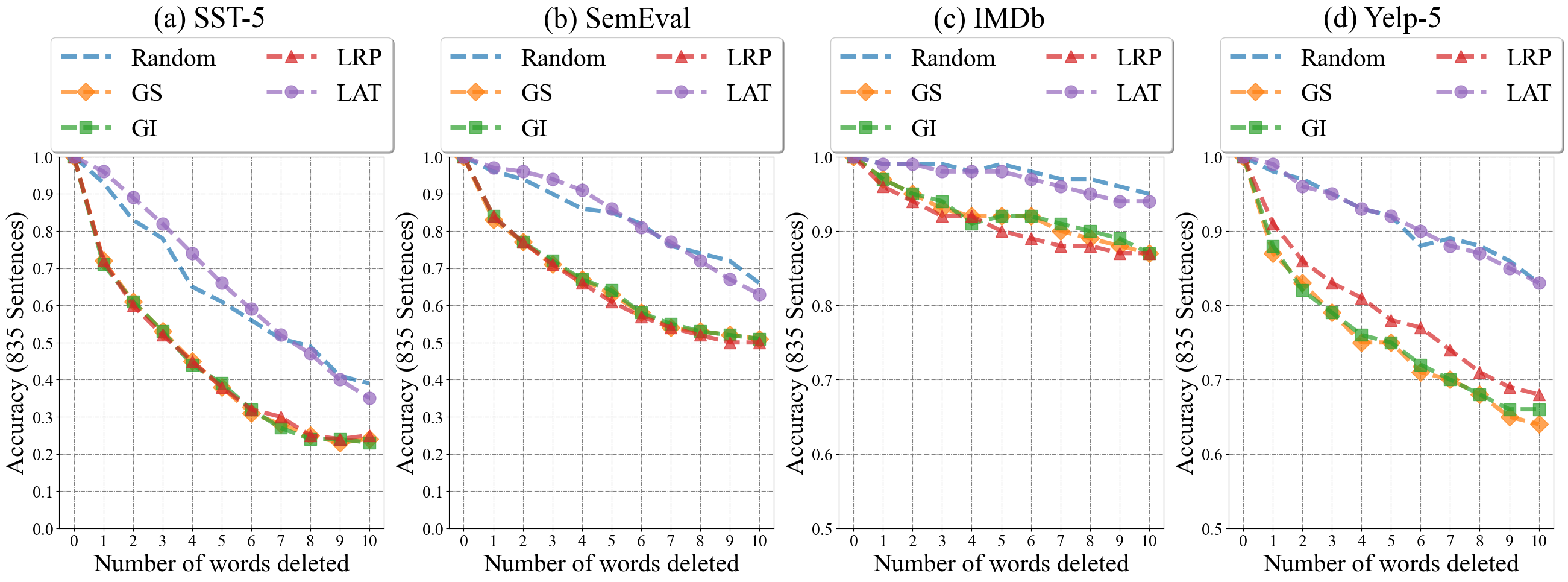
Figure 1: Accuracy v.s. Number of words deleted on initially correctly classified sentences in test sets for all datasets, using attribution methods including Gradient Sensitivity (GS), Gradient $\times$ Input (GI), Layerwise Relevance Propagation (LRP) and Layerwise Attention Tracing (LAT). We also include random word deletion as a baseline.

Dataset	GS	GI	LRP	LAT
SST-5	0.91	0.91	0.89	0.85
SemEval	0.89	0.88	0.83	0.81
IMDb	0.81	0.82	0.81	0.79
Yelp-5	0.83	0.86	0.79	0.73

Table 1: Correlations of relevance scores across two models trained with different initializations.

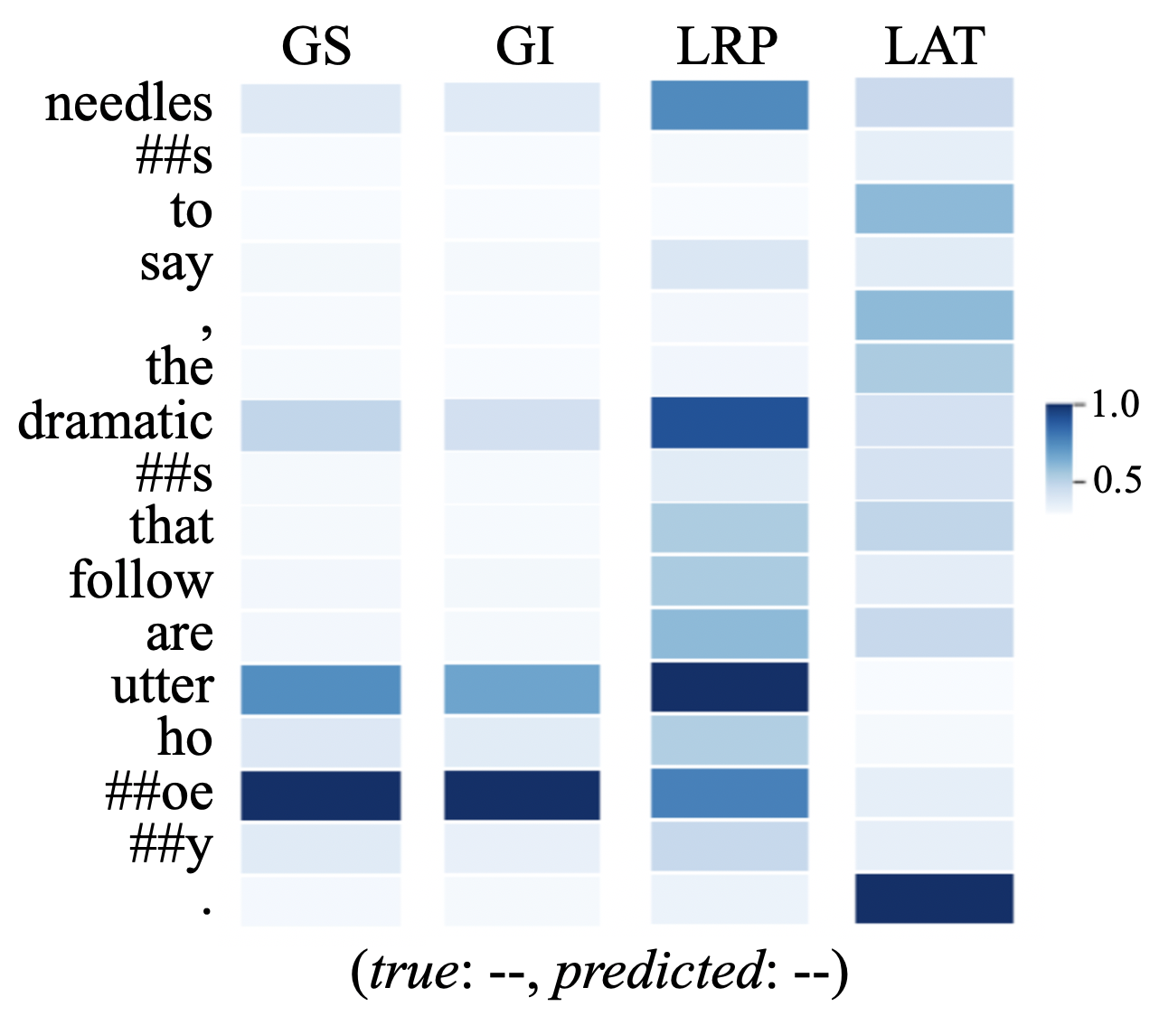
Figure 2: Examples of relevance scores generated using four introduced methods. The model predicts correctly, where the true label of this sentence is very negative (–).

3 Models

We first fine-tuned a BERT model with a classification head for each sentiment analysis dataset from a distinct domain: SST-5 (short sequence movie reviews) Socher et al. (2013), SemEval Rosenthal et al. (2017) (short sequence tweets), IMDb Review Maas et al. (2011) (long sequence movie reviews) and Yelp Review (long sequence restaurant reviews) Zhang et al. (2015). For additional details on set-ups, see Appendix C.

4 Experiment

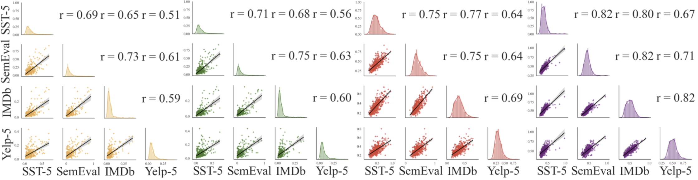
Figure 3: Correlations of relevance scores derived from four attribution methods across four datasets.

4.1 Performance and Relevance Scores

We first used each attribution method to calculate relevance scores tokens of sentences in each test set. Fig. 2 presents a sentence with token-level relevance scores. Our results suggest that LRP shows richer variance in terms of relevance scores, and encodes richer semantic properties (i.e., all words with strong emotional semantics are highlighted). GS and GI show similar patterns but with more pin-pointed focuses. On the other hand, LAT seems to distract to irrelevant words. Table 2 presents top 5 words and bottom 5 words ranked by their relevance scores for each attribution method. For details on other datasets, see Appendix D.

We further quantified the validity of each attribution methods via an ablation study where we successively remove words in the descending order of relevance scores with in sequence. Fig. 1 shows model accuracy drops consistently by removing important words across each dataset. Our results suggest that GS, GI and LRP present similar trends in changes of performance, whereas LAT is close to the trend of random word dropping. This further suggests that LAT may be ineffective in retrieving relevance scores within a sequence.

GS	GI	LRP	LAT
mess	mess	repetitive	repetitive
disturbing	slick	lacks	in
slick	disturbing	anything	disturbing
fine	fine	hilarious	lacks
laugh	miss	thriller	stupid
ka	create	post	el
create	ka	close	des
were	were	el	lo
ni	the	ga	ka
michael	michael	ca	ho

Table 2: Top and bottom 5 words ranked by averaged relevance scores derived from each method for SST-5 test. Each words appear at least 5 times.

4.2 Robustness with Random Initialization

Recent works suggest that fine-tuning is susceptible to random initializations, where model performances may vary significantly. In this vein, we tested whether relevance scores are susceptible with random initializations. We retrained our model with different initialization, and correlate relevance scores. Table 1 shows Pearson Correlations Benesty et al. (2009) of relevance scores under two different initializations of our fine-tuning process. Our results suggest that random initializations affect our results but only to a limited extend. Furthermore, consistencies in results of longer sentences seem to suffer more from random initializations comparing to shorter ones.

4.3 Consistency across Datasets

We then tested whether attribution methods can explain generalizable semantics through relevance scores across multiple datasets that share similar semantics. We first took a common vocabulary across four datasets, and calculated Pearson Correlations Benesty et al. (2009) of relevance scores for shared words in the vocabulary. Fig. 3 presents correlation matrices across four datasets for each attribution methods. Surprisingly, four methods show strong correlations across four datasets, even for LAT which performs poorly in our ablation tests. This suggests that learnt weights in BERT may be generalizable across tasks with similar semantics.

5 Related Works

Attribution methods were used to explain BERT in sequence to sequence modelings. For instance, previous works showed that heads can be ranked and pruned via importance scores derived using LRP Voita et al. (2019). In parallel, recent works used LRP to explain linguistic properties learnt by BERT for machine translation tasks Voita et al. (2020). Others applied gradient-based methods and attention weights-based methods to study linguistic properties encoded in self-attention layers Hao et al. (2020); Wu et al. (2020). Attribution methods are also widely used for explaining other neural networks such as MLP Li et al. (2016) and LSTM Arras et al. (2017).

6 Conclusions

In this paper, we adapt four existing attribution methods with BERT models for four sequence classification tasks that share similar semantics. Furthermore, we both qualitatively and quantitatively compare the validity and robustness for these four different methods across our datasets. More importantly, we show that attribution methods generalize well across tasks with shared semantics. Our works provide an initial guidance in selecting attribution methods for BERT-based models for downstream probing tests on classification tasks.

Appendix

Appendix A Non-linear Activations

Point-wise monotonic activation functions are ignored by LRP as the estimated gradients for these layer are not changed for a given $x$. We are aware that the GeLU activations Hendrycks and Gimpel (2016) in BERT is not strictly monotonically increasing, and we leave this for the future to investigate potential drawbacks of ignoring this in BERT. We split the test set evenly if the original dataset does not come with a dev set.

Appendix B Gradient-based methods and LRP

In this section, we present connections between gradient-based attribution methods (e.g., GS or GI) and LRP. First, let us rewrite our Eqn. 1 using chain-rule as Bach et al. (2015):

$$\mathbf{R}^{\text{GS}}_{i}(x)=\frac{\partial f_{c}(x)}{\partial x_{i}^{l}}\frac{\partial x_{i}^{l}}{\partial x_{i}^{l-1}}\cdots\frac{\partial x_{i}^{1}}{\partial x_{i}}$$ (11)

where $x_{i}^{l}$ are intermediate hidden states in different layers. Let us consider the simplest case where the neural network contains only linear layers with non-linear activation functions $g(\cdot)$ as in Eqn. 3 to  4. We can then rewrite Eqn. 11 as:

$$\mathbf{R}^{\text{GS}}_{i}(x) =\mathbf{w}^{l}g^{\prime}(z_{j}^{l+1})\cdots\mathbf{w}^{0}g^{\prime}(z_{j}^{1})$$ (12)

$$=(\prod_{l}\mathbf{w}^{l})(\prod_{l}g^{\prime}(z_{j}^{l+1}))$$ (13)

where $g^{\prime}(\cdot)$ is the derivatives of non-linear activation functions. For GI, we need to append the input features to the front as in Eqn. 2:

$$\mathbf{R}^{\text{GI}}_{i}(x) =x_{i}(\prod_{l}\mathbf{w}^{l})(\prod_{l}g^{\prime}(z_{j}^{l+1}))$$ (14)

To reiterate our formulation for LRP as in Eqn. 7:

$$\mathbf{R}^{\text{LRP}}_{i}(x) =f_{c}(x)(\prod_{l}\frac{\mathbf{w}^{l}x^{l}}{z^{l+1}})(\prod_{l}g^{\prime}(\mathbf{z}_{j}^{l+1}))$$ (15)

where, if we ignore non-linear activation functions, Shrikumar et al. (2017) showed that absent modifications for numerical stability, vanilla LRP rules were equivalent within a scaling factor of GS. See Shrikumar et al. (2017) for a comprehensive proof.

Appendix C Datasets and Models

We fine-tuned BERT with four datasets separately. Table 3 presents statistics of our datasets. Table 3 shows model performance for each dataset. Our results show that all of our models achieved the state-of-the-art performance Wang et al. (2018).

Our fine-tune begins with the uncased BERT-base parameters  and adds a n-way sentiment classifier head. During fine-tuning, BERT-base is trained for 3 epochs where the best model is recorded. As in the original BERT-base model (Liu et al., 2019), our model consists 12 heads and 12 layers, with hidden layer size 768. The model uses the default BERT WordPiece tokenizer, with a maximum sequence length of 512. The initial learning rate is $2e^{-5}$ for all trainable parameters, with a batch size of 8 per device (i.e., GPU). We fine-tuned for 3 epochs with a dropout probability of 0.1 for both attention weights and hidden states. The Best model is chosen based on performance on the respective dev set.

We used 6 $\times$ GeForce RTX 2080 Ti GPU each with 11GB memory to fine-tune. The fine-tuning process takes from 1 hour to 10 hours to finish from the smallest dataset to the largest one.

Dataset	Train	Dev	Test	Acc /%
SST-5	156,817	1,101	2,210	56.9
SemEval	39,656	2,478	2,478	74.2
IMDb	24,999	12,500	12,499	89.0
Yelp-5	649,999	25,000	24,999	66.0

Table 3: Datasets with model performances.

Appendix D Word Rankings

These tokens are from randomly sampled 2000 sentences from SST-5, and at least appear five times. The reason to filter words based on frequency is that we want to have more stable results by taking the average relevance score across many occurrences. We also exclude punctuation marks in the Table 2 by focusing on words which are linguistically interesting. Table 4 to  6 provide tables with top 5 and bottom 5 words ranked by relevance scores for other three datasets for comparison.

GS	GI	LRP	LAT
weird	weird	excited	in
sad	nice	awesome	undertaker
nice	sad	jurassic	to
sweet	sweet	amazing	fleetwood
excellent	excellent	happy	excited
co	29	green	sy
29	co	return	wo
30	30	stream	mi
48	48	fr	je
ar	21	en	ac

Table 4: Top 5 words followed by bottom 5 words with ranked by averaged relevance scores based on different attribution methods for SemEval test. Each words appear at least 5 times. Punctuation marks are skipped.

GS	GI	LRP	LAT
succeeds	succeeds	simpsons	mtv
nightmare	perfection	emotionally	countless
joke	nightmare	mtv	emotionally
creep	joke	animated	everyday
perfection	creep	immensely	include
passed	passed	fist	br
rave	rose	semi	mon
rose	ernest	stu	ac
ernest	rave	mon	mar
pac	feet	cad	hal

Table 5: Top 5 words followed by bottom 5 words with ranked by averaged relevance scores based on different attribution methods for IMDb test. Each words appear at least 5 times. Punctuation marks are skipped.

GS	GI	LRP	LAT
tooth	tooth	waitress	email
edible	edible	amazing	amazing
superb	superb	disappointing	dessert
thrilled	grade	detail	convenience
pink	odd	disgusting	upset
tar	tar	tar	lu
tree	tree	rico	ha
lu	lu	nr	ni
keeping	national	trees	z
ke	keeping	nun	ke

Table 6: Top 5 words followed by bottom 5 words with ranked by averaged relevance scores based on different attribution methods for Yelp-5 test. Each words appear at least 5 times. Punctuation marks are skipped.

References

- Abnar and Zuidema (2020) Samira Abnar and Willem Zuidema. 2020. Quantifying attention flow in transformers. In Proceedings of the 58th Annual Meeting of the Association for Computational Linguistics, pages 4190–4197, Online. Association for Computational Linguistics.
- Arras et al. (2017) Leila Arras, Grégoire Montavon, Klaus-Robert Müller, and Wojciech Samek. 2017. Explaining recurrent neural network predictions in sentiment analysis. In Proceedings of the 8th Workshop on Computational Approaches to Subjectivity, Sentiment and Social Media Analysis, pages 159–168.
- Bach et al. (2015) Sebastian Bach, Alexander Binder, Grégoire Montavon, Frederick Klauschen, Klaus-Robert Müller, and Wojciech Samek. 2015. On pixel-wise explanations for non-linear classifier decisions by layer-wise relevance propagation. PloS one, 10(7).
- Benesty et al. (2009) Jacob Benesty, Jingdong Chen, Yiteng Huang, and Israel Cohen. 2009. Pearson correlation coefficient. In Noise reduction in speech processing, pages 1–4. Springer.
- Böhle et al. (2019) Moritz Böhle, Fabian Eitel, Martin Weygandt, and Kerstin Ritter. 2019. Layer-wise relevance propagation for explaining deep neural network decisions in mri-based alzheimer’s disease classification. Frontiers in aging neuroscience, 11:194.
- Clark et al. (2019) Kevin Clark, Urvashi Khandelwal, Omer Levy, and Christopher D Manning. 2019. What does BERT look at? An analysis of BERT’s attention. In Proceedings of the 2019 ACL Workshop BlackBoxNLP: Analyzing and Interpreting Neural Networks for NLP, pages 276–286.
- Clark et al. (2020) Kevin Clark, Minh-Thang Luong, Quoc V Le, and Christopher D Manning. 2020. Electra: Pre-training text encoders as discriminators rather than generators. arXiv preprint arXiv:2003.10555.
- Devlin et al. (2019) Jacob Devlin, Ming-Wei Chang, Kenton Lee, and Kristina Toutanova. 2019. BERT: Pre-training of deep bidirectional transformers for language understanding. In Proceedings of the 2019 Conference of the North American Chapter of the Association for Computational Linguistics: Human Language Technologies.
- Goldberg (2019) Yoav Goldberg. 2019. Assessing BERT’s syntactic abilities. arXiv preprint arXiv:1901.05287.
- Hao et al. (2020) Yaru Hao, Li Dong, Furu Wei, and Ke Xu. 2020. Self-attention attribution: Interpreting information interactions inside transformer. arXiv preprint arXiv:2004.11207.
- Hendrycks and Gimpel (2016) Dan Hendrycks and Kevin Gimpel. 2016. Gaussian error linear units (gelus). arXiv preprint arXiv:1606.08415.
- Hewitt and Manning (2019) John Hewitt and Christopher D Manning. 2019. A structural probe for finding syntax in word representations. In Proceedings of the 2019 Conference of the North American Chapter of the Association for Computational Linguistics: Human Language Technologies, Volume 1 (Long and Short Papers), pages 4129–4138.
- Kindermans et al. (2017) Pieter-Jan Kindermans, Sara Hooker, Julius Adebayo, Maximilian Alber, Kristof T Schütt, Sven Dähne, Dumitru Erhan, and Been Kim. 2017. The (un) reliability of saliency methods. arXiv preprint arXiv:1711.00867.
- Li et al. (2016) Jiwei Li, Xinlei Chen, Eduard Hovy, and Dan Jurafsky. 2016. Visualizing and understanding neural models in NLP. In Proceedings of the 2016 Conference of the North American Chapter of the Association for Computational Linguistics: Human Language Technologies.
- Liu et al. (2019) Yinhan Liu, Myle Ott, Naman Goyal, Jingfei Du, Mandar Joshi, Danqi Chen, Omer Levy, Mike Lewis, Luke Zettlemoyer, and Veselin Stoyanov. 2019. Roberta: A robustly optimized bert pretraining approach. arXiv preprint arXiv:1907.11692.
- Maas et al. (2011) Andrew Maas, Raymond E Daly, Peter T Pham, Dan Huang, Andrew Y Ng, and Christopher Potts. 2011. Learning word vectors for sentiment analysis. In Proceedings of the 49th annual meeting of the association for computational linguistics: Human language technologies, pages 142–150.
- Raganato and Tiedemann (2018) Alessandro Raganato and Jörg Tiedemann. 2018. An analysis of encoder representations in Transformer-based machine translation. In Proceedings of the 2018 EMNLP Workshop BlackboxNLP: Analyzing and Interpreting Neural Networks for NLP, pages 287–297.
- Rosenthal et al. (2017) Sara Rosenthal, Noura Farra, and Preslav Nakov. 2017. SemEval-2017 task 4: Sentiment analysis in Twitter. In Proceedings of the 11th International Workshop on Semantic Evaluation (SemEval-2017), pages 502–518, Vancouver, Canada. Association for Computational Linguistics.
- Shrikumar et al. (2017) Avanti Shrikumar, Peyton Greenside, and Anshul Kundaje. 2017. Learning important features through propagating activation differences. In Proceedings of the 34th International Conference on Machine Learning, volume 70 of Proceedings of Machine Learning Research, pages 3145–3153, International Convention Centre, Sydney, Australia. PMLR.
- Socher et al. (2013) Richard Socher, Alex Perelygin, Jean Wu, Jason Chuang, Christopher D Manning, Andrew Y Ng, and Christopher Potts. 2013. Recursive deep models for semantic compositionality over a sentiment treebank. In Proceedings of the 2013 Conference on Empirical Methods in Natural Language Processing, pages 1631–1642.
- Tenney et al. (2019) Ian Tenney, Dipanjan Das, and Ellie Pavlick. 2019. Bert rediscovers the classical nlp pipeline. In Proceedings of the 57th Annual Meeting of the Association for Computational Linguistics, pages 4593–4601.
- Vig and Belinkov (2019) Jesse Vig and Yonatan Belinkov. 2019. Analyzing the structure of attention in a transformer language model. In Proceedings of the 2019 ACL Workshop BlackboxNLP: Analyzing and Interpreting Neural Networks for NLP, pages 63–76.
- Voita et al. (2020) Elena Voita, Rico Sennrich, and Ivan Titov. 2020. Analyzing the source and target contributions to predictions in neural machine translation. arXiv preprint arXiv:2010.10907.
- Voita et al. (2018) Elena Voita, Pavel Serdyukov, Rico Sennrich, and Ivan Titov. 2018. Context-aware neural machine translation learns anaphora resolution. In Proceedings of the 56th Annual Meeting of the Association for Computational Linguistics, pages 1264–1274.
- Voita et al. (2019) Elena Voita, David Talbot, Fedor Moiseev, Rico Sennrich, and Ivan Titov. 2019. Analyzing multi-head self-attention: Specialized heads do the heavy lifting, the rest can be pruned. In Proceedings of the 57th Annual Meeting of the Association for Computational Linguistics, pages 5797–5808, Florence, Italy. Association for Computational Linguistics.
- Wang et al. (2018) Alex Wang, Amanpreet Singh, Julian Michael, Felix Hill, Omer Levy, and Samuel Bowman. 2018. Glue: A multi-task benchmark and analysis platform for natural language understanding. In Proceedings of the 2018 EMNLP Workshop BlackboxNLP: Analyzing and Interpreting Neural Networks for NLP, pages 353–355.
- Wu et al. (2020) Zhengxuan Wu, Thanh-Son Nguyen, and Desmond Ong. 2020. Structured self-AttentionWeights encode semantics in sentiment analysis. In Proceedings of the Third BlackboxNLP Workshop on Analyzing and Interpreting Neural Networks for NLP, pages 255–264, Online. Association for Computational Linguistics.
- Yang et al. (2018) Yinchong Yang, Volker Tresp, Marius Wunderle, and Peter A Fasching. 2018. Explaining therapy predictions with layer-wise relevance propagation in neural networks. In 2018 IEEE International Conference on Healthcare Informatics (ICHI), pages 152–162. IEEE.
- Yang et al. (2019) Zhilin Yang, Zihang Dai, Yiming Yang, Jaime Carbonell, Russ R Salakhutdinov, and Quoc V Le. 2019. Xlnet: Generalized autoregressive pretraining for language understanding. In Advances in neural information processing systems, pages 5753–5763.
- Zhang et al. (2015) Xiang Zhang, Junbo Zhao, and Yann LeCun. 2015. Character-level convolutional networks for text classification. Advances in neural information processing systems, 28:649–657.