Abstract

We have analyzed the Barrow holographic dark energy (BHDE) in the framework of the flat FLRW Universe by considering the various estimations  of Barrow exponent $\triangle$. Here we define BHDE, by applying the usual holographic principle at a cosmological system, for utilizing  the Barrow entropy rather than the standard Bekenstein-Hawking. To understand the recent accelerated expansion of the universe, considering  the Hubble horizon as the IR cut-off. The cosmological parameters, especially the density parameter ($\Omega_{{}_{D}}$), the equation of the state  parameter ($\omega_{{}_{D}}$), energy density ($\rho_{{}_{D}}$) and the deceleration parameter($q$) are studied in this manuscript and found  the satisfactory behaviors. Moreover, we additionally focus on the two geometric diagnostics, the statefinder $(r,s)$ and $O_{m}(z)$ to discriminant  BHDE model from the $\Lambda CDM$ model. Here we determined  and plotted the trajectories of evolution for statefinder $(r,s)$, $(r,q)$ and  $O_{m}(z)$ diagnostic plane to understand the geometrical behavior of the BHDE model by utilizing Planck 2018 observational information. Finally, we have explored the new Barrow exponent $\triangle$, which strongly affect the  dark energy equation of state that can lead it to lie in the quintessence regime, phantom regime, and exhibits the phantom-divide line during the cosmological evolution.

Keywords: FLRW universe, Barrow HDE, Hubble horizon, Statefinder diagnostic
PACS: 98.80.-k, 98.80.Jk,

1 Introduction

The well-proven accelerated expansion of the universe is the greatest achievement of $20^{th}$ century [1, 2]. The dark energy (DE) with immense negative pressure is considered one of the mysterious reasons behind the accelerated expansion of the universe. The WMAP experiment also suggests that the Universe is made up of $4\%$ of the Baryonic matter, $23\%$ DM and $73\%$ DE [3]. In the path of expansion, the universe passes through different phases of DE/matter. The DE is typically defined by the EoS parameter $(\omega)$  and the ranges include $-1/3<\omega<-1$ for quintessence, $\omega<-1$ for phantom and $(\omega=1)$ for the cosmological constant.

Recently, researchers show a great interest in HDE models, since these HDE models developed as applications of DE by following holographic principle [4]. The holographic principle derives from the thermodynamics of the black hole. String theory provides a relation between the IR cutoff of quantum field theory linked to vacuum energy  [4]-[7]. This concept has been utilized widely in cosmological contemplations, especially in the late-time period of the Universe, at present known as, holographic dark energy models [8]-[22]. During this phase, we would like to mention that  Nojiri-Odintsov cut-off [8] gave the most general holographic dark energy and it is intriguing that it might be applied to covariant hypotheses [23]. So for solving the dark energy puzzle, (HDE) speculation is a promising approach [16]-[18]. The new HDE models can be proposed by utilizing holographic speculation and a generalized entropy. In addition to the dark energy model, it is also found that the HDE is important to analyze the early evolution of the Universe, such as the inflationary evolution [24]-[29]. It is worth mentioned here some latest papers [30]-[35] and their references on HDE in various scenarios.

In this present work, we consider a spatially flat, homogeneous, and isotropic spacetime as the underlying geometry. Here we study the behavior of different cosmological parameters (the deceleration parameter, the energy density parameter, and the equation of state parameter ) during the cosmic evolution by assuming the Hubble horizon as the infrared (IR) cut-off. The Hubble horizon as an IR cut-off is suitable to clarify the ongoing accelerated expansion of the DE models.

In this direction, many cosmologists have presented mathematical diagnostics ${r,s}$, known as statefinder parameters. For observing the nature of DE models, statefinder parameters are the most important parameter [36]-[37]. In order to discriminate the various DE models, the trajectories can be represented graphically in $r-s$ and $r-q$ planes. The state finder parameters are also analyzed [38, 39]. DE models like Chaplygin gas models, quintessence model, cosmological constant and braneworld model as explored in [40] -[44].

Barrow holographic dark energy (BHDE) is also a fascinating alternative scenario for the quantitative description of DE which is based on the holographic hypothesis [45]-[49]  and applying the recently proposed Barrow entropy [50] instead of the normal Bekenstein-Hawking [51, 52]. Saridakis [53] have shown that the BHDE includes basic HDE as a sub-case in the limit where Barrow entropy becomes the usual Bekenstein-Hawking. Anagnostopoulos et al. [54] have shown that the BHDE is an agreement with observational data, and it can serve as a good candidate for the description of DE. Barrow holographic dark energy models have been studied by several authors [55] -[60] in different contexts.

On the other hand, concerning various cosmological theories, where DE interacts with DM has extended much attention in the literature [61].

The essential aspect in holographic principle in the cosmological level, is that the universe Horizon entropy is proportional to its area, as similar to the Bekenstein-Hawking entropy, with a black hole. The entropy of the black hole shown by Barrow can be modified as [50]

$$S_{B}=\left(\frac{B}{B_{0}}\right)^{1+\frac{\triangle}{2}}~{}~{}~{}~{}~{}0\leq\triangle\leq 1,$$ (1)

where $B_{0}$ is the Planck area and $B$ is the normal horizon area.

There is a quantum-gravitational deformation which enumerated by the parameter $\triangle$ , for $\triangle=0$  related to the Bekenstein-Hawking standard entropy and $\triangle=1$ corresponding to the most complex and fractal structure.  The aim of the present manuscript is to examine the BHDE model by taking the Hubble radius as an IR cutoff and analyzing the  behavior of cosmological parameters for a flat FRW universe. We extend our analysis to BHDE, inspired by the works [53] with a similar  IR cut-off which gives the ongoing stage progress of the Universe. We get the statefinder parameters for BHDE which accomplish the  worth of $\Lambda CDM$  model and show consistency with the quintessence model for appropriate estimation of parameters. The plan of  this manuscript is as follow: In section $2$, we introduce the BHDE model proposed in [53] with a general interaction term between  the dark components (BHDE and DM) of the universe and also study its cosmological evolution by considering the basic field equations.  The behavior of state finder pair for BHDE has been discussed in section $3$, we explore the $O_{m}$ diagnostic in section $4$. Finally,  section $5$ is devoted to conclusions.

2 Basic field Equations

In this section we develop the scenario of Barrow holographic dark energy, where the inequality $\rho_{{}_{D}}L^{4}\leqslant S$, is given by the standard HDE. Here $L$ is the horizon length under the assumption $S\propto A\propto L^{2}$ [9] by using the Barrow entropy (1) obtain as lead to

$$\rho_{{}_{D}}=CL^{\triangle-2},$$ (2)

where $C$ is a parameter with dimensions $[L]^{-2-\triangle}$ and $L$ denotes the IR cutoff. In the case where $\triangle=0$ as expected, the above expression provides the standard holographic dark energy $\rho_{D}=3c^{2}M_{p}^{2}L^{-2}$ (here $M_{p}$ is the Plank mass), where $C=3c^{2}M_{p}^{2}$ and with the model parameter $c^{2}$. The above relation leads to some interesting results in the holographic and cosmological setups [53, 54]. In [62, 56], Barrow entropy was added in the structure of “gravity-thermodynamics” conjecture, according to which the first law of thermodynamics can be applied on the universe apparent horizon. As a result, one obtains a modified cosmology, with extra terms in the Friedmann equations depending on the new exponent $\triangle$, which disappear in the case $\triangle=0$, i.e when Barrow entropy becomes the standard Bekenstein-Hawking one. Although this framework is defined in a very effective way in the universe of late time. It should be noted here that the value $\triangle=1$ corresponds to the maximal deformation, while the value $\triangle=0$ corresponds to the simplest horizon structure, and the normal Bekenstein entropy [51, 52] can be recovered in this case. It is essential to note here that the entropy in equation (1), is close to Tsallis’ non-extensive entropy [63, 64]. In the case where the deformation effects are quantified with $\triangle$, Barrow holographic dark energy will leave the regular one, leading to numerous cosmological variations. Recently, Barrow et al. [62] have used Big Bang Nucleosynthesis (BBN) data in order to impose constraints on the exponent of Barrow entropy. They have shown that the Barrow exponent should be inside the bound $\triangle\lesssim 1.4\times 10^{-4}$ in order not to spoil the BBN epoch.

Therefore, the BHDE is surely a more general structure than the standard HDE scenario. Here we concentrate on the general case of $(\triangle>0)$. If we assumed that the Hubble horizon $H^{-1}$ as the IR cutoff $(L)$, we can write the energy density of BHDE as

$$\rho_{{}_{D}}=CH^{2-\triangle}$$ (3)

Let us consider a spatially flat, homogeneous and isotropic, FLRW universe the standard metric is given by

$$ds^{2}=-dt^{2}+a^{2}(t)(dr^{2}+r^{2}d\Omega^{2})$$ (4)

In a flat FLRW Universe, the field equations for BHDE are given as :

$$H^{2}=\frac{1}{3}8\pi G(\rho_{{}_{D}}+\rho_{m})\\$$ (5)

where $\rho_{{}_{D}}$ is the energy density of BHDE and $\rho_{m}$ is the energy

density of matter respectively. The energy density parameter of BHDE and matter can be given as $\Omega_{m}=\frac{8\pi\rho_{m}G}{3H^{2}}$ and $\Omega_{{}_{D}}=\frac{8\pi\rho_{{}_{D}}G}{3H^{2}}$.

We know that the relation

$$\Omega_{{}_{BD}}+\Omega_{m}=1$$ (6)

The conservation law BHDE and matter are defined as :

$$\dot{\rho}_{m}+3H\rho_{m}=0$$ (7)

$$\dot{\rho}_{{}_{D}}+3H(p_{{}_{D}}+\rho_{{}_{D}})=0$$ (8)

From Eq. (3), we get

$$\dot{\rho}_{{}_{D}}=\frac{3C}{2}(2-\triangle)H^{2-\triangle}\left(\frac{\Delta\Omega_{D}}{(\Delta-2)\Omega_{D}+2}-1\right)$$ (9)

Now, Eqs. (5), (7) and (8) and combining the outcome with the Eq. (6), we obtained

$$\frac{\dot{H}}{H^{2}}=\frac{3}{2}\left(\frac{\Delta\Omega_{D}}{(\Delta-2)\Omega_{D}+2}-1\right)$$ (10)

The deceleration parameter $q$ is written as

$$q=-1-\frac{\dot{H}}{H^{2}}$$ (11)

By using Eq. (10), the deceleration parameter $q$ is also written as

$$q=\frac{1-(\Delta+1)\Omega_{D}}{(\Delta-2)\Omega_{D}+2}.$$ (12)

By utilizing the Eq. (8) with Eqs. (9) and (10), we get the expression for the EoS parameter derived as:

$$\omega_{D}=-\frac{\Delta}{(\Delta-2)\left(1-\frac{(z+1)^{3}\Omega_{\text{m0}}}{-\Omega_{\text{m0}}+(z+1)^{3}\Omega_{\text{m0}}+1}\right)+2},$$ (13)

where dash is the derivative, here we differentiate the EoS parameter $\omega_{{}_{D}}$ with respect to $lna$ then we get $\omega_{{}_{D}}^{{}^{\prime}}$. By using the Eqs. (9) and (10), we find

$$\omega^{{}^{\prime}}_{D}=-\frac{3\Delta^{3}\left(\Omega_{D}-1\right)\Omega_{D}}{\left((\Delta-2)\Omega_{D}+2\right){}^{3}}.$$ (14)

Similarly by using the Eqs. (9) and (10), we obtained $\Omega_{{}_{D}}$ as:

$$\Omega^{{}^{\prime}}_{D}=-\frac{3\Delta\Omega_{D}\left(\Omega_{D}-1\right)}{(\Delta-2)\Omega_{D}+2}$$ (15)

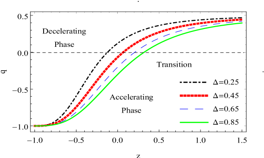
Figure 1: Plot of deceleration parameter $(q)$ with redshift $z$

The evolution of $q$ has been plotted in Fig. $1$. As we observed from Fig. $1$, the BHDE model can explain the universe’s history very well, with the sequence of an early matter-dominated era. Here we plot the  $q$ versus $z$ for a various choice of Barrow exponent $\triangle$. Which explains that the model is stable in the era of matter dominance.  Moreover, we analyzed that in the high redshift phase, we have $q\to-1$, while at $z\to-1$. It is worth mentioning that, cosmos may cross the phantom line ($q<-1$) for $z<-1$ depending on the value of $\triangle$. The decelerating parameter approaches positive to negative values when the universe is overcome by dark energy. However, our findings based on the different values of the $\triangle$. If we take $\triangle=0.25,0.45,0.65,0.85$ the decelerating parameter $q$ is deceleration   to accelerating for the present time. Additionally, the transition redshift $z_{t}=0$ occurs within the interval $-0.25<z_{t}<0.25$, which are in good compatibility with different  recent studies (see Refs. [65]-[71] for more details  about the models and cosmological datasets used). It has also been observed that the parameter $z_{t}$ depends on  the values of $\triangle$ in such a way that, as  $\triangle$  increases, the  parameter $z_{t}$ also increases. According to the Planck measurement of $\Omega_{D}$, the value of $r$ is $0.445\pm 0.010$.

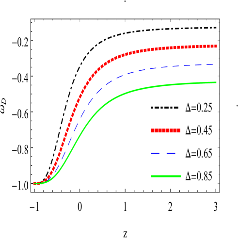
Figure 2: Plot of EoS parameter ($\omega_{{}_{D}}$) with redshift $z$

Next, we have shown the evolution of the EoS parameter $\omega_{{}_{D}}$ in Fig. $2$ by considering different values of $\triangle$ with respect to redshift $z$. The expression for equation of state parameter $\omega_{{}_{D}}$ represents in Eq. (13). One of the main efforts in observational cosmology is the measurement of EoS for dark energy (DE). Interestingly, we observed that for different values of $\triangle$, the EoS parameter $\omega_{{}_{D}}$ lies in the quintessence regime $(\omega_{{}_{D}}>-1)$ at the present epoch, however it enters in the phantom regime $(\omega_{{}_{D}}<-1)$  in the far future (i.e.,$z\to-1$). On the other hand, we also observed from the figure that the EoS parameter was very close to zero at high redshift and attains some $-ve$ value in between the region $-1$ to $-1/3$ at low redshift and further settles to a value very close to $-1$ in the far future. In this way, we see,  according to the value of $\triangle$, Barrow holographic dark energy can lie in the quintessence or in the the phantom regime, or exhibit the phantom-divide crossing during the cosmological evolution.

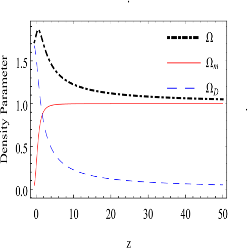
Figure 3: Plot of density parameter ($\Omega_{{}_{D}}$) with redshift $z$

In this segment, we discuss cosmological development in the scenario of Barrow holographic dark energy. Figure $3$ shows the evolution of the BHDE density parameter $\Omega_{{}_{D}}$ as a function of the redshift parameter $z$. From Fig. $2$, it is evident that $\Omega$ approaches unity as the universe evolves to high redshift, and Where $\Omega_{{}_{D}}$  is the density parameter for BHDE, and the $\Omega_{m}$ represents the density parameter of matter. By the assumption, [72], it has been seen that the current universe is near a spatially at geometry  ($\Omega\approx 1$). This really is a characteristic outcome from inflation in the early universe [73]. Our figure depicts  that as $z\to 0$, $\Omega>1$ or $\Omega<1$ and when $z\to\infty$, $\Omega=1$.

3 Statefinder

In order to get a vigorous investigation to separate among DE models, many authors [36, 37] have presented a new mathematical diagnostic pair ${(r,s)}$, known as statefinder parameter, which is developed from the scale factor. These parameters ${(r,s)}$ is geometrical in the behavior and it is developed from the space-time metric directly.

The dynamics of the universe are comprehensively described by statefinder $(r,s)$. These are determined as

$$r=\frac{\dddot{a}}{aH^{3}}$$ (16)

$$s=\frac{(r-1)}{3(q-\frac{1}{2})}$$ (17)

The relation between the statefinder parameters $r$ and $s$ in terms of energy density can be expressed as

$$r=\frac{(\Delta(\Delta(\Delta+12)-6)-8)\Omega_{D}^{3}+3(\Delta(4-7\Delta)+8)\Omega_{D}^{2}+3(\Delta-2)(3\Delta+4)\Omega_{D}+8}{\left((\Delta-2)\Omega_{D}+2\right){}^{3}}$$ (18)

$$s=-\frac{2\left(\Omega_{D}-1\right)\left(2(\Delta-1)\Omega_{D}-\Delta+2\right)}{\left((\Delta-2)\Omega_{D}+2\right){}^{2}}$$ (19)

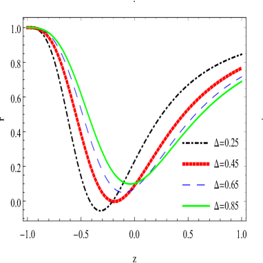
(a) (b)

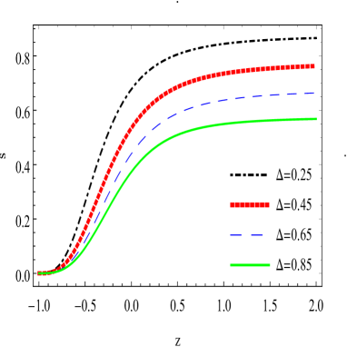
Figure 4: (a) Plot of $r$ with redshift $z$ (b) Plot of $s$ with redshift $z$

The evolution of $r$ and $s$ with redshift $z$ for FLRW universe has been analyzed in Figs. $4a$ and $4b$ [74]. The primary parameter $r$ of Oscillating dark energy (ODE), at high redshift, approaches standard $\Lambda CDM$ behavior while at low redshift it goes deviates significantly from the standard behavior and the second parameter $s$ shows opposite in behavior [75]. Figures $4a$ and $4b$ portray evaluation of $r$ and $s$ for different values of Barrow parameter $\triangle$ and approaches to the $\Lambda CDM$, by taking the value (for $\Omega_{m_{0}}$ = $0.27$ and $H_{0}$= $69.5$) are in good arrangement with recent observations. As expected, for $\triangle=0$ the above modified Friedmann equations reduce to $\Lambda CDM$ scenario.  The study of the statefinder provides a very useful method to split the conceivable depravity of different cosmological models by  determining the parameters $r$, and $s$ for the higher order of the scale factor.

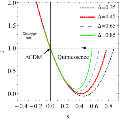
(a) (b)

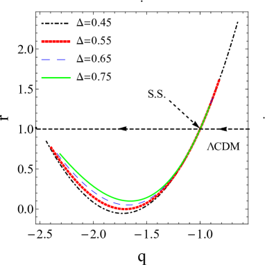
Figure 5: (a) Plot of $(r-s)$ with $z$ (b) Plot of $(r-q)$ with $z$

In Fig. $5a$, we plot  $r-s$ trajectories which divided into two regions. The region $r>1$, $s<0$ in the $r-s$ plane, shows a behaviour similar to a Chaplygin gas (CG) model [76] whereas the region $r<1$,  $s>0$ shows a behaviour similar to the quintessence model (Q- model) [36, 37]. However, the model shows a behavior of CG at early time for $\triangle=0.25,0.45,0.65,0.85$ and approaches $\Lambda CDM$  at late times. The trajectories in both region coincide for all different values of $\triangle$. The statefinder ${r,s}$ of BHDE model approaches to the $\Lambda CDM$. In addition, we also plot the evolution trajectory in the $r-q$ plane in figure $5b$. The $(r-q)$ trajectories are divided into two regions through the point $(r,q)=(1,-1)$. The region $r>1$, $q<-1$ in the $r-q$ plane shows a behaviour similar to the phantom model, while the region $r<1$ $q>-1$ shows a behaviour similar to quintessence (Q-model). In this figure, the arrow represents the fixed points at ${r,q}={1,-1}$ of the steady-state (SS) model. As exhibited in [42]-[54] the statefinder can effectively separate between a wide assortment of DE models including the quintessence, phantom, quintom,  cosmological constant, braneworld models, Chaplygin gas, and interacting DE models.

4 $O_{m}(z)$ Diagnostics

The Om diagnostic analysis is also a very useful geometrical diagnosis that can be used for such analysis. In the investigation of the statefinder parameter $(r,s)$ the higher order derivative of $a(t)$ are utilized. The Ist order derivative are used in $O_{m}$ diagnostic analysis because it contains only the Hubble parameter.

The $O_{m}$ diagnostic can be considered as an easier diagnostic [77]. It might be noticed that the $O_{m}$ diagnostic has been additionally applied to [78]-[80]. This arrangement of parameters can be written as:

$$Om(z)=\frac{\frac{H^{2}(z)}{H_{0}}-1}{(1+z)^{3}-1}$$ (20)

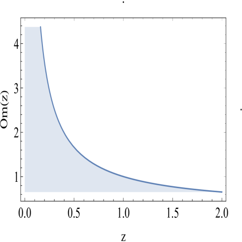
Figure 6: Plot of $O_{m}(z)$ with redshift $z$

In figure $6$, we plot the $O_{m}(z)$ evolution with redshift. The positive curve of the $O_{m}(z)$ trajectories shows the phantom behaviour $(\omega<-1)$ whereas the negative curve implies that DE behaves like quintessence $(\omega>-1)$. We noticed in our figure, when the redshift z is expanding inside the stretch $0<z<2.0$, the $O_{m}(z)$ is diminishing monotonically and the curve lies in phantom region. The new diagnostic of dark energy $O_{m}$ is acquainted with separate $\Lambda CDM$ from other DE models. Where $H_{0}$ is the current estimation of the Hubble parameter. Here we demonstrated that the slope of $O_{m}(z)$ can recognize dynamical DE from the cosmological consistent in a robust way.

5 Conclusion

In this model, we have discussed the BHDE, by considering the typical holographic principle at a cosmological system, by utilizing the Barrow entropy, rather than the standard Bekenstein-Hawking. Here we have also discussed the evolution of a spatially flat FLRW universe composed of pressure less dark matter and Barrow holographic dark energy. By considering the Hubble horizon as the infrared cut-off, we have found the exact solution and the calculated cosmological parameters like the behavior of the density parameter, the EoS parameter, the deceleration parameter, statefinder, and $O_{m}$ diagnostic parameters, etc. We also plotted the trajectories in $(r-s),(r-q)$, and $O_{m}$  to discriminate the various DE model from the existing BHDE models during the cosmic evolution.

The main highlights of the models are as per the following:

• It has been found that the BHDE model exhibits a   smooth transition from early deceleration era $(q>0)$ to   the present acceleration $(q<0)$  era of the universe in Fig. $1$.  Also,   the value of this transition redshift is in good accordance   with the current cosmological observations and obtained for the different values of the $\triangle$.

• It has  been  observed in Fig. $2$ that the new Barrow exponent $\triangle$ essentially influences the dark energy equation   of state and as per its worth it lies in the quintessence regime $(\omega_{D}>-1)$, at the current era, however it enters in   the phantom regime $(\omega_{D}<-1)$  in the far future (i.e.,$z\to-1$)   by using different values of $\triangle$.

• The energy density parameter is also discussed and shown in Fig. $3$. We found that in the cosmic evaluation of BHDE $\Omega$, approaches unity.   which is a good agreement with recent observations.

• We have also discussed the statefinder $(r,s)$  in terms of the dimensionless density parameters and Barrow exponent $\triangle$.   We have plotted  $r$ verses $z$ in Fig. $4a$. The  $r(z)$ parameter of oscillating dark energy (ODE) depicts in  high red shift region   and  approaches to standard $\Lambda CDM$. Similarly we have obtained $s(z)$  in Fig. $4b$, where $s(z)$ parameter shows opposite behaviour   to the primary parameter $r$.

• The excellent diagnostics of DE is shown in Figs. $5a$ and $5b$ which are ${(r,s)}$ and ${(r,q)}$.  Here we take the value     $\Omega_{m_{0}}=0.27$, $H_{0}=69.5$ and  using the different values of $(\triangle=0.25,0.45,0.65,0.85)$, then the   averaged-over-redshift statefinder pair ${(r,s)}$ and ${(r,q)}$ obtained the Chaplygin gas (CG) model, steady state (SS) model,   quintessences (Q-model) etc. Now we observe that the statefinders play a very important role in the FLRW universe with BHDE.

• The $O_{m}$-diagnostic technique is used to check the stability of the model and various periods of the Universe. We plot   the trajectory in Om(z)plane to separate the conduct of the DE models in Fig. $6$. The positive inclination  of the curve shows   the phantom-like behavior of the model

In summary, in the manuscript, the physical behavior of the cosmological parameters are studied through their graphical representation.  This BHDE model is in a good agreement with cosmological informations, and it can fill in as a decent possibility for the graphical representation.

6 Acknowledgments

The author (AP) thanks the IUCAA, Pune, India for providing the facility under visiting associateship. The authors are also thankful to the anonymous referee for his/her constructive comments which helped to improve the quality of paper in present form.

References

- [1] A. G. Riess, et al., Observational evidence from supernovae for an accelerating universe and cosmological constant, Astron. J. 116, (1998) 1009.
- [2] S. Perlmutter, et al., Measurements of omega and lambda from 42 high-redshift supernovae, Astrophys. J. 517, (1999) 565.
- [3] C. Bennett, First-Year Wilkinson Microwave Anisotropy Probe (WMAP) Observations: Foreground Emission, Astrophys. J. Suppl. Ser. 148, (2003) 1.
- [4] L. Susskind, The world as a hologram, J. Math. Phys. 36, (1995) 6377.
- [5] G. ’t Hooft, Dimensional reduction in quantum gravity, Conf. Proc. C 284, (1993) 930308, gr-qc/9310026.
- [6] E. Witten, Anti-de Sitter space and holography, Adv. Theor. Math. Phys. 253, (1998), hep-th/9802150.
- [7] R. Bousso, The holographic principle, Rev. Mod. Phys. 74 , (2002) 825.
- [8] S. Nojiri, S. D. Odintsov, Unifying phantom inflation with late-time acceleration: scalar phantom–non-phantom transition model and generalized holographic dark energy, Gen. Rel. Grav. 38, (2006) 1285.
- [9] S. Wang, Y.Wang, M. Li, Holographic dark energy, Phys. Rept. 696, (2017) 1.
- [10] M. Li, A model of holographic dark energy, Phys. Lett. B 603, (2004) 1.
- [11] E. N. Saridakis, Restoring holographic dark energy in brane cosmology, Phys. Lett. B 660, (2008) 138.
- [12] D. Pavon, W. Zimdahl, Holographic dark energy and cosmic coincidence, Phys. Lett. B 628, (2005) 206.
- [13] X. Zhang, Statefinder diagnostic for holographic dark energy model, Int. J. Mod. Phys. D 14, (2005) 1597.
- [14] E. Elizalde, S. Nojiri, S. D. Odintsov, P. Wang, Dark energy: vacuum fluctuations, the effective phantom phase, and holography, Phys. Rev. D 71, (2005) 103504.
- [15] M. Li, C. Lin, Y. Wang, Some issues concerning holographic dark energy, JCAP 0805, (2008) 023.
- [16] M. Bouhmadi-Lopez, A. Errahmani, T. Ouali, Cosmology of a holographic induced gravity model with curvature effects, Phys. Rev. D 84, (2011) 083508.
- [17] Y.G. Gong, B. Wang, Y.Z. Zhang, Holographic dark energy reexamined, Phys. Rev. D 72, (2005) 043510.
- [18] Y. Gong, T. Li, A modified holographic dark energy model with infrared infinite extra dimension (s), Phys. Lett. B 683, (2010) 241.
- [19] M. Malekjani, Generalized holographic dark energy model in the Hubble length, Astrophys. Space Sci. 347 (2013) 405.
- [20] R. C. G. Landim, Holographic dark energy from minimal supergravity, Int. J. Mod. Phys. D 25, (2016) 1650050.
- [21] M. Khurshudyan, J. Sadeghi, R. Myrzakulov, A. Pasqua, H. Farahani, Interacting quintessence dark energy models in Lyra manifold, Adv. High Energy Phys. 2014, (2014) 878092.
- [22] C. Gao, F. Wu, X. Chen, Y. G. Shen, Holographic dark energy model from Ricci scalar curvature, Phys. Rev. D 79, (2009) 043511.
- [23] S. Nojiri, S. Odintsov, Covariant generalized holographic dark energy and accelerating universe, Eur. Phys. J. C 77, (2017) 528.
- [24] S. Nojiri, S.D. Odintsov, E. N. Saridakis, Holographic inflation, Phys. Lett. B 797, (2019) 134829.
- [25] T. Paul, Holographic correspondence of gravity with/without matter fields, Europhys. Lett. 127, (2019) 20004.
- [26] A. Bargach, F. Bargach, A. Errahmani, T. Ouali, Induced gravity effect on inflationary parameters in a holographic cosmology, Int. J. Mod. Phys. D 29, (2020) 2050010.
- [27] R. Horvat, Holographic bounds and Higgs inflation, Phys. Lett. B, 699, (2011) 174.
- [28] E. Elizalde, A. Timoshkin, Viscous fluid holographic inflation, Eur. Phys. J. C 79, (2019) 732.
- [29] A. Oliveros, M. A. Acero, Inflation driven by a holographic energy density, Europhys. Lett. 128, (2019) 59001.
- [30] S. Ghaffari, Holographic dark energy model in the DGP brane world with time varying holographic parameter, New Astron. 67, (2019) 76.
- [31] S. Ghaffari, A. A. Mamon, H. Moradpour, A. H. Ziaie, Holographic dark energy in Rastall theory, Mod. Phys. Lett. A 35, (2020) 2050276.
- [32] V. Srivastava, U. K. Sharma, Statefinder hierarchy for Tsallis holographic dark energy, New Astron. 78, (2020) 101380.
- [33] U. K. Sharma, V. C. Dubey, Statefinder diagnostic for the Renyi holographic dark energy, New Astron. 80, (2020) 101419.
- [34] S. H. Shekh, S. D. Katore, V. R. Chirde, S. V. Raut, Signature flipping of isotropic homogeneous space-time with holographic dark energy in gravity, New Astron. 84, (2021) 101535.
- [35] U. K. Sharma, V. Srivastava, Tsallis HDE with an IR cutoff as Ricci horizon in a flat FLRW universe, New Astron. 84, (2021) 101519.
- [36] V. Sahni, T. D. Saini, A. A. Starobinsky, U. Alam, Statefinder-a new geometrical diagnostic of dark energy, J. Exp. Theo. Phy. Lett. 77 , (2003) 201, arXiv:astro-ph/0201498.
- [37] U. Alam, V. Sahni, T. D. Saini, A. A. Starobinsky, Exploring the expanding universe and dark energy using the statefinder diagnostic, Mon. Not. R. Astron. Soc. 344 (2003) 1057, arXiv: astro-ph/0303009.
- [38] M. Malekjani, A. Khodam-Mohammadi, N. Nazari-pooya, Cosmological evolution and statefinder diagnostic for new holographic dark energy model in non flat universe, Astrophys. Space Sci. 332 (2011) 515, arXiv:1011.4805[gr-qc].
- [39] U. Debnath, S. Chattopadhyay, Statefinder and diagnostics for interacting new holographic dark energy model and generalized second law of thermodynamics, Int. J. Theo. Phy. 52, (2013) 1250.
- [40] M. R. Setare, J. Zhang, X. Zhang, Statefinder diagnosis in non-flat universe and the holographic model of dark energy, JCAP 03, (2007) 007.
- [41] M. Malekjani, A. Khodam-Mohammadi, Statefinder diagnosis and the interacting ghost model of dark energy, Astrophys. Space Sci. 343, (2013) 451.
- [42] A. Dixit, U. K. Sharma, A. Pradhan, Tsallis holographic dark energy in FRW universe with time varying deceleration parameter, New Astron. 73, (2019) 101281.
- [43] V. C. Dubey, U. K. Sharma, A. Beesham, Tsallis holographic model of dark energy: cosmic behaviour, statefinder analysis and pair in the non-flat universe, Int. J. Mod. Phys. D 28, (2019) 1950164.
- [44] C. J. Feng, Statefinder diagnosis for Ricci dark energy, Phys. Lett. B 670, (2008) 231.
- [45] R. Bousso, The holographic principle for general backgrounds, Class. Quantum Grav. 17, (2000) 997.
- [46] H. Kim, H. W. Lee, Y. S. M. Kim, Equation of state for an interacting holographic dark energy model, Phys. Lett. B 632, (2006) 605.
- [47] W. Fischler, L. Susskind, Holography and cosmology, arXiv: hep-th/9806039 (1998).
- [48] A. Cohen, D. Kaplan, A. Nelson, Effective field theory, black holes, and the cosmological constant, Phys. Rev. Lett. 82, (1999) 4971.
- [49] P. Horava, D. Minic, Probable values of the cosmological constant in a holographic theory, Phys. Rev. Lett. 85, (2000) 1610.
- [50] J. D. Barrow, The area of a rough black hole, Phys. Lett. B 808, (2020) 135643.
- [51] J. D. Bekenstein, Black holes and the second law, Lett. Nuovo Cimento 4, (1972) 737.
- [52] J. D. Bekenstein, Black holes and entropy, Phys. Rev. D 7, (1973) 2333.
- [53] E. N. Saridakis, Barrow holographic dark energy, arXiv: 2005.04115 (2020).
- [54] F. K. Anagnostopoulos, S. Basilakos, E. N. Saridakis, Observational constraints on Barrow holographic dark energy, arXiv: 2005.10302 (2020).
- [55] S. Srivastava, U. K. Sharma, Barrow holographic dark energy with Hubble horizon as IR cutoff, New Astron. arXiv: 2010.09439[physics.gn-ph] (2020).
- [56] E. N. Saridakis, Modified cosmology through spacetime thermodynamics and Barrow horizon entropy, arXiv: 2006.01105[gr-qc] (2000).
- [57] A. A. Mamon, A. Paliathanasis, S. Saha, Dynamics of an Interacting Barrow Holographic Dark Energy Model and its Thermodynamic Implications, arXiv: 2007.16020[gr-qc] (2000).
- [58] E. M. C. Abreu, J. A. Neto, Barrow black hole corrected-entropy model and Tsallis nonextensivity, Phys. Lett. B 810, (2020), 135805.
- [59] S. N. Saridakis, S. Basilakas, The generalized second law of thermodynamics with Barrow entropy, arXiv: 2005.08258[gr-qc] (2000).
- [60] E. M. C. Abreu, J. A. Neto, Barrow fractal entropy and the black hole quasinormal modes, Phys. Lett. B 807, (2020), 135602.
- [61] Y. L. Bolotin, A. Kostenko, O. A. Lemets, D. A.Yerokhin, Cosmological evolution with interaction between dark energy and dark matter, Int. J. Mod. Phys. D 24, (2015) 1530007.
- [62] J. D. Barrow, S. Basilakos and E. N. Saridakis, Big Bang Nucleosynthesis constraints on Barrow entropy, arXiv: 2010.00986v1 [gr-qc] (2020)
- [63] C. Tsallis, Possible generalization of Boltzmann-Gibbs statistics, J. Statist. Phys. 52, (1988) 479.
- [64] C. Tsallis and L. J. L. Cirto, Black hole thermodynamical entropy, Eur. Phys. J. C 73, (2013) 2487.
- [65] O. Farooq, B. Ratra, Hubble parameter measurement constraints on the cosmological deceleration-acceleration transition redshift, The Astroph. J. Lett. 766, (2013) L7.
- [66] O. Farooq, F. R. Madiyar, S. Crandall, B. Ratra, Hubble parameter measurement constraints on the redshift of the deceleration-acceleration transition, dynamical dark energy, and space curvature, Astro. J. 835, (2017) 26.
- [67] A. A. Mamon, Constraints on a generalized deceleration parameter from cosmic chronometers, Mod. Phys. Lett. A 33, (2018) 1850056.
- [68] A. A. Mamon, K. Bamba, Observational constraints on the jerk parameter with the data of the Hubble parameter, Eur. Phys. J. C 78, (862) (2018) 1.
- [69] A. A. Mamon, S. Das, A divergence-free parametrization of deceleration parameter for scalar field dark energy, Int. J. Mod. Phys. D. 25, (2016) 1650032.
- [70] A. A. Mamon, S. Das, A parametric reconstruction of the deceleration parameter, Eur. Phys. J. C 77, (2017) 495.
- [71] J. Magana, V. H. Cardenas, V. Motta, Cosmic slowing down of acceleration for several dark energy parametrizations, J. Cosmol. Astropart. Phys. 2014, (2014) 017, arXiv:1407.1632[astro-ph.CO].
- [72] D. N. Spergel, et al. [WMAP Collaboration], Wilkinson microwave anisotropy probe (WMAP) three year results: Implications for cosmology, Astrophys. J. Suppl. 170, (2007) 377.
- [73] A. R. Lindle, D. H. Lyth, Cosmological in ation and large scale structure, Cambridge University Press (2000).
- [74] S. L. Cao, Song Li, Hao-Ran Yu, Tong-Jie Zhang, Statefinder diagnostic and constraints on the palatini gravity theories, Res. Astron. Astrophys. 18 , (2018) 026.
- [75] G. Panotopoulos, A. Rincon, Growth index and statefinder diagnostic of oscillating dark energy, Phys. Rev. D 97, (2018) 103509.
- [76] Y. B. Wu, S. Li, M. Hui Fu, Jing He, A modified Chaplygin gas model with interaction, Gen. Rel. Grav. 39, (2007) 653.
- [77] M. Shahalam, S. Sami, A. Agarwal, diagnostic applied to scalar field models and slowing down of cosmic acceleration, Mon. Not. Roy. Astron. Soc. 448, (2015) 2948.
- [78] M. Jamil, D. Momeni, R. Myrzakulov, Observational constraints on non-minimally coupled Galileon model, Eur. Phys. J. C 73, (2013) 2347.
- [79] Paul De Fromont, Claudia De Rham, Lavinia Heisenberg, Andrew Matas, Superluminality in the bi-and multi-Galileon, J. High Energy Phys. 2013, (2013) 67.
- [80] V. Sahni, A. Shafieloo, A. A.Starobinsky, Two new diagnostics of dark energy, Phys. Rev. D 78, (2008)103502.