Task Offloading and Resource Allocation with Multiple CAPs and Selfish Users

Abstract

In this work, we consider a multi-user mobile edge computing system with multiple computing access points (CAPs). Each mobile user has multiple dependent tasks that must be processed in a round-by-round schedule. In every round, a user may process their individual task locally, or choose to offload their task to one of the $M$ CAPs or the remote cloud server, in order to possibly reduce their processing cost. We aim to jointly optimize the offloading decisions of the users and the resource allocation decisions for each CAP over a global objective function, defined as a weighted sum of total energy consumption and the round time. We first present a centralized heuristic solution, termed MCAP, where the original problem is relaxed to a semi-definite program (SDP) to probabilistically generate the offloading decision. Then, recognizing that the users often exhibit selfish behavior to reduce their individual cost, we propose a game-theoretical approach, termed MCAP-NE, which allows us to compute a Nash Equilibrium (NE) through a finite improvement method starting from the previous SDP solution. This approach leads to a solution from which the users have no incentive to deviate, with substantially reduced NE computation time. In simulation, we compare the system cost of the NE solution with those of MCAP, MCAP-NE, a random mapping, and the optimal solution, showing that our NE solution attains near optimal performance under a wide set of parameter settings, as well as demonstrating the advantages of using MCAP to produce the initial point for MCAP-NE.

I Introduction

With the ever-increasing demand for computational resources by mobile applications, from a variety of tasks including machine learning, virtual reality, and natural language processing, there is a growing need for accessible computational resources in mobile networks that are available for task offloading [2]. Mobile Cloud Computing (MCC) would allow mobile devices to offload tasks to large remote data centres in the cloud, such as Amazon EC2 [3]. This promises to improve the performance of demanding mobile applications and expand the computational capabilities of mobile devices for future applications.

However, MCC systems may cause high latency for these mobile users, due to the transmission delays required to wirelessly offloading tasks through long distances in order to reach the remote server. This can prove fatal in providing adequate quality of service of many applications, especially computationally-intensive real-time ones such as virtual reality. One means of resolving this is by providing additional wireless and/or computational resources at the edge of the mobile system, such as the wireless base station, thus giving the users faster access to the necessary resources [4], [5], [6]. Because base stations have high-speed connections to the Internet and thus the various cloud servers, offloading through these edge hosts could substantially reduce the transmission time and energy required to access these servers. Additionally, base stations may hold their own servers, providing mobile users with an additional site for possible task offloading. When computational resources are installed at or near radio access networks, the system paradigm is known as Mobile Edge Computing (MEC), as defined by the European Telecommunications Standards Institute (ETSI) [6]. However, other similar systems, such as micro cloud centers, [7], cloudlets [8], and fog computing [9], use similar methods to reduce the communication latency that result from MCC.

When these computing resources are built into a wireless access point or cellular base station, we refer to it as a computing access point (CAP) [10], [11], [12], [13]. The CAP performs two functions—it serves as a link between the individual mobile devices and the remote cloud server, whereby the application can be forwarded through a high-speed connection, and it serves as an additional site for the computation of the task itself, if doing so is more beneficial than local or remote processing.

One research problem that arises from MCC and MEC systems is that of the offloading decision—how to determine whether a task should be executed on the user’s mobile device, or offloaded to the available edge or cloud servers [5]. Additionally, the available bandwidth and computational resources are limited, especially at the CAP—thus good system performance would require a judicious distribution of these resources between the users. Ideally, the offloading decision and the resource allocation would be jointly optimized in order to maximize the overall quality of service provided by the system to the users. However, this is a difficult problem due to the multiple tiers of offloading available, the heterogeneous resources that must be assigned, the asymmetrical nature of the system, and the need to optimize over a set of binary offloading decisions, resulting in a mixed-integer programming problem that is non-convex and difficult to solve.

In [10], a single CAP and remote cloud server system were considered, with multiple users and one atomic task per user to be offloaded. A centralized controller was designed to jointly optimize the offloading decisions and resource allocations to minimize a weighted sum of total energy consumption and the time required to process all of the tasks (i.e. the round time). The problem was formulated as a mixed-integer optimization problem, and using semidefinite relaxation (SDR) techniques from [14], a heuristic solution was presented and shown through simulation to perform near optimally under a wide range of system parameters.

However, in practical systems often multiple CAPs are simultaneously available to the users. This added dimension in the solution space adds significant complexity to the offloading decision and resource allocation decisions, especially since the computational capability of different CAPs, as well as the quality of wireless access to them, can substantially differ. Furthermore, the centralized optimization model does not account for any agency of the users in making these offloading decisions, who often exhibit selfish behaviour in reality, where each individual user would choose the offloading site that minimizes their own individual cost. In such cases, individual users would not have an incentive to follow the decisions of the central controller, limiting the scope of [10].

In this work, we consider a multi-user system with a remote cloud server and multiple CAPs. Each user has a single task per round, which may be processed at the user’s mobile device, or offloaded it to one of the CAPs, where it may be processed either directly or further offloaded to the remote cloud server. The goal is to choose a set of offloading and resource allocation decisions that minimize the system cost or objective, which we define as a weighted sum of energy consumption and the round time, as in [10] and [11]. We further aim to ensure that selfish users have no incentive to deviate from their prescribed offloading decisions.

The contributions of our work are as follows:

• We develop the MCAP heuristic by modelling the above optimization problem as a quadratically-constrained quadratic program (QCQP), extending the single-CAP formulation in [10] to multiple CAPs. To do so, we must make significant changes to the formulation in [10], particularly through new objective variables and constraints to accommodate the additional offloading possibilities. We also accommodate for the addition of placement constraints, which prevent user from offloading their task through some CAPs. We then relax the problem to produce a semidefinite program (SDP), and use those results to probabilistically produce a series of offloading decisions, following the work in [14]. We choose the decisions among those trials that minimizes the system cost.

• We then consider the phenomenon of selfish users, where individual users in the system may deviate from the centralized decisions in order to minimize their individual costs. Utilizing game theory, we show that the multi-CAP system with selfish users can be modeled as a strategic finite game with an ordinal potential function, which allows us to compute a Nash Equilibrium (NE) through the finite improvement method [15]. While a game-theoretic approach may suffer from an additional price of anarchy, the NE provides overall system performance that is close to the optimal solution.

• However, due to the combinatorial nature of the finite improvement method, solving for the NE may require substantial computational time. To reduce the number of iterations required, we propose using a starting point that is closer to the optimal solution than a randomly chosen one. We use MCAP to obtain such a starting point, which is then combined with the finite improvement method to construct the MCAP-NE solution. Thus, MCAP-NE improves on MCAP by further reducing the system cost and accounting for the agency of selfish users. Simulation results demonstrate the superiority of the SDR approach in MCAP over a random set of offloading decisions, the further improvements from the game-theoretic approach in MCAP-NE, the close proximity of these solutions to the optimal solution of the system, and the computational improvements due to the MCAP starting point, under a wide range of parameter settings.

Our paper is organized as follows. Section 2 reviews related works in solving the offloading problem in MEC systems. Section 3 formulates the problem and system model, culminating in a centralized optimization problem. Section 4 reformulates the system as a QCQP, which is then optimized heuristically through an SDR approach, to be used as the initial starting point for our NE solution method. Section 5 then reformulates the problem as a strategic form game, proves the existence of an ordinal potential function and NE, and presents an algorithm to find the NE. Section 6 presents our numerical results. Finally, Section 7 concludes the paper.

II Related Works

While there are many existing works that study the offloading problem in two-tier cloud systems, including [16], [17], [18], [19] and [20], among others, fewer works have studied three tier offloading networks. Such works include [10], [11], [12], [13], [21], [22], [23], and [24]. However, [21], [22], [23], and [24] only consider the offloading decision and do not attempt to optimize the resource allocation. Joint optimization over the offloading decisions and the resource allocation is studied in [10] (and its extension in [11]) and [12] (and its extension in [13]) where a multi-user, single CAP system with a remote cloud server is considered. These works present a heuristic centralized solution using SDR for the offloading of one and multiple tasks per round respectively, with delay constraints also being considered in [11]. As stated above, in this work we consider the more complex problem of multiple CAPs and add the assumption of selfish users to solve the problem using both SDR and game theory.

Game-theoretic approaches to analyzing mobile offloading networks have been presented in [24], [25], [26], [27], [28], [29], [30], [31], and [32]. All of these works except [24] and [25] consider a single atomic task per user, which is similar to our work, while [24] and [25] stand apart for considering a Poisson generation of user tasks and a queueing system for offloading. All of these works except [26] study systems with potential functions and utilize that fact in the computation of an NE. While the system in [26] is not a potential game, their proof of the existence of an NE relies on the fact that a subgame within their system is a potential game, and they utilize that fact to modify the finite improvement method in order to produce an algorithm that could find the NE of the overall game.

In [27] and [28], the finite improvement method from [15] is directly adopted. These works however do not consider the practical implementation of the finite improvement method, which is expressly considered in [29] and [30], where a decentralized solution was presented. In these works, each user computes their improvements locally, using a pilot signal to determine the the interference at the wireless channel (which entails all of the necessary information to the user), and a base station that coordinates the transmission of this signal between the users. A similar method is proposed in [31], where the computation of the improvements are computed by the individual users, with a central controller coordinating these computations between the users and disclosing the relevant information to them. The finite improvement method is further improved in [31] by demonstrating theoretical limits to the available strategies for each user that may result in an improvement. Another decentralized approach is considered in [32], where each user first adopts a mixed strategy, then uses reinforcement learning to converge to a pure strategy NE. Thus, [32] does not use the finite improvement method utilized by the other above works to compute the NE—however, [32] still relies on the existence of an ordinal potential function to demonstrate the convergence of their solution method to the NE.

In this work, we adopt a centralized approach to computing the NE, which allows the system to compute an initial starting point to reduce the overall computational time. Furthermore, we demonstrate that our system is strategy-proof, thus ensuring that users have no incentive to provide false information to the controller, which guarantees the viability of a centralized approach. More importantly, none of these works considers a three-tier computing systems. In particular, in the offloading systems of [27] and [29] (with a single wireless access point), or [26], [28], [30], [31], and [32] (with multiple wireless access points), the wireless access points serve only to forward the offloaded tasks to the cloud. Therefore, their offloading and resource allocation solutions are not applicable to our problem.

III System Model and Centralized Optimization

In this section, we develop the system model in question, denoting all the relevant variables and modeling the cost of processing at every offloading site. From this, we arrive at a mixed-integer programming problem to minimize the overall cost of the system.

Consider a cloud access network consisting of one remote cloud server, $M$ CAPs denoted by the set $\mathcal{M}\in\{1,\ldots,M\}$, and $N$ mobile users denoted by the set $\mathcal{N}\in\{1,\ldots,N\}$, as shown in Fig. 1. Each mobile user may have multiple tasks to be processed, and we consider a round-by-round schedule where one task from each user is processed in each round. No task in the next round may begin processing until all the tasks of the current round have been processed in the system. Because of this condition, it suffices to optimize the offloading decisions and resources allocation for mobile users in a single round. This will be the focus of the remainder of the work, and without loss of generality we assume there are $N$ tasks in this round.

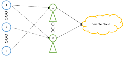
Figure 1: A mobile cloud system with CAPs.

III-A Offloading Decision

In each round, a user may process their task locally, or offload it to one of the $M$ CAPs. Each user $i$ has a possibly empty set of $\mathcal{K}_{i}\subset\mathcal{M}$ CAPs to which they may not offload their task to. If a task is offloaded to a CAP, it may be processed there or further offloaded to the remote cloud server. Denote the offloading decision of user $i$ by

$$\mathbf{x}_{i}=[x_{i0},x_{i1},\ldots,x_{iM}] \in\{0,1\}^{M+1},$$ (1)

$$\theta_{i} \in\{0,1\},$$ (2)

where $x_{i0}=1$ if its task is locally processed locally at the user’s own device, $x_{ij}=1,j>0$ if the task is offloaded to CAP $j$ , and $\theta_{i}=1$ if the task that is offloaded to a CAP is processed at the cloud. We assume that the tasks are atomic and cannot be placed in multiple locations, only one of $x_{i0},x_{i1},\ldots,x_{iM}$ can be active — this can be expressed through the following constraint:

$$\sum_{j=0}^{M}x_{ij}=1,\forall i\in\mathcal{N}.$$ (3)

Additionally, processing at the cloud can only happen through transmission from one of the CAPs—thus $\theta_{i}\neq 1$ if $x_{i0}=1$. Alternately,

$$\theta_{i}\leq\sum_{j=1}^{M}x_{ij},\quad\forall i\in\mathcal{N}.$$ (4)

Finally, the placement constraints of each user are expressed as follows:

$$x_{ik}=0,\quad\forall k\in\mathcal{K}_{i},i\in\mathcal{N}.$$ (5)

III-B Cost of Local Processing

The input data size, output data size, and required number of processing cycles of user $i$’s task are denoted by $D_{{\text{in}}}(i)$, $D_{{\textrm{\text{out}}}}(i)$, and $Y(i)$, respectively. For local computation, the processing time required is $T_{i}^{L}$, and the energy consumption for the user is $E_{i}^{L}$.

III-C Cost of CAP Processing

For tasks processed at a CAP, the bandwidth and processing rate that is allocated to each user must be determined in order to compute the energy and time required to complete a task. Each CAP has its own wireless channel where users may offload their tasks to. The uplink transmission time is given as

$$T_{ij}^{t}=\frac{D_{\text{in}}(i)}{\eta_{ij}^{u}c_{ij}^{u}},$$ (6)

where $c_{ij}^{u}$ is the uplink bandwidth to CAP $j$ assigned to user $i$, and $\eta_{ij}^{u}$ is the spectral efficiency of the uplink transmission from user $i$ to CAP $j$. The downlink transmission time is given as

$$T_{ij}^{r}=\frac{D_{\text{out}}(i)}{\eta_{ij}^{d}c_{ij}^{d}},$$ (7)

where $c_{ij}^{d}$ and $\eta_{ij}^{d}$ is the respective downlink bandwidth and spectral efficiency. The bandwidths $c_{ij}^{u}$ and $c_{ij}^{d}$ are further limited by bandwidth capacities as follows:

$$\sum_{i=1}^{N}c_{ij}^{u}\leq C_{j}^{\text{UL}},\quad\forall j\in\mathcal{M},$$ (8)

$$\sum_{i=1}^{N}c_{ij}^{d}\leq C_{j}^{\text{DL}},\quad\forall j\in\mathcal{M},$$ (9)

$$\sum_{i=1}^{N}(c_{ij}^{u}+c_{ij}^{d})\leq C_{j}^{\text{Total}},\quad\forall j\in\mathcal{M}.$$ (10)

Furthermore, a task is processed at the CAP with processing time $T_{ij}^{a}=Y(i)/f_{ij}^{a}$, where $f_{ij}^{a}$ is the processing rate at CAP $j$ assigned to user $i$, and constrained by the total processing rate of the CAP:

$$\sum_{i=1}^{N}f_{ij}^{a}\leq f_{j}^{A},\quad\forall j\in\mathcal{M}.$$ (11)

The total time required for processing task $i$ on CAP $j$ can then be expressed as

$$T_{ij}^{A}=T_{ij}^{t}+T_{ij}^{r}+T_{ij}^{a}.$$ (12)

The energy consumption required for CAP processing can be expressed as

$$E_{ij}^{A}=E_{ij}^{t}+E_{ij}^{r},$$ (13)

where $E_{ij}^{t}$ and $E_{ij}^{r}$ represent the uplink and downlink transmission energy costs required by the user, respectively.

III-D Cost of Cloud Processing

For cloud processing, the uplink and downlink transmission energies and times are identical to the CAP processing case. However, there is now further transmission time between the CAP and the cloud, expressed as $T_{i}^{ac}=(D_{\text{in}}(i)+D_{\text{out}}(i))/r_{ac}$, where $r_{ac}$ is a predetermined wired transmission rate between the CAPs and the cloud. The computation time is $T_{i}^{c}=Y(i)/f_{i}^{C}$, where $f_{i}^{C}$ is a predetermined processing rate assigned to each user at the cloud. Thus, the total cloud processing time can be expressed as

$$T_{ij}^{C}=T_{ij}^{t}+T_{ij}^{r}+T_{i}^{ac}+T_{i}^{c}.$$ (14)

The energy consumption can be expressed as

$$E_{ij}^{C}=E_{ij}^{t}+E_{ij}^{r}+\beta_{i}C_{i}^{C},$$ (15)

where $C_{C_{i}}$ is the cloud utility cost, and $\beta_{i}$ is the relative weight.

TABLE I: Parameters and Respective Descriptions.

Parameter	Description
$E_{i}^{L}$	local processing energy of user $i$’s task
$E_{ij}^{t}$, $E_{ij}^{r}$	uplink transmitting energy and downlink
	receiving energy of user $i$’s task to and
	from CAP $j$, respectively
$T_{i}^{L}$, $T_{i}^{C}$	local processing time and cloud processing
	time of user $i$’s task, respectively
$T_{ij}^{t}$, $T_{ij}^{t}$	uplink transmission time and downlink
	transmission time of user $i$’s task between
	a mobile user and CAP $j$, respectively
$T_{i}^{ac}$	transmission time of user $i$’s task between
	CAP and cloud
$C^{\text{UL}}_{j}$, $C^{\text{DL}}_{j}$, $C^{\text{Total}}_{j}$	uplink, downlink, and total transmission
	capacity associated with CAP $j$, respectively
$c_{ij}^{u}$, $c_{ij}^{d}$	uplink and downlink bandwidth
	assigned to user $i$ from CAP $j$
$f_{ij}^{a}$	CAP processing rate assigned to user $i$ from
	CAP $j$
$\eta_{ij}^{u}$, $\eta_{ij}^{d}$	uplink and downlink spectral efficiency
	from user $i$ to CAP $j$
$C_{i}^{C}$	system utility cost of user $i$’s task
$r_{ac}$	transmission rate for each user
	between the CAP and cloud
$f_{i}^{C}$	cloud processing rate for each user

These various parameters are summarized in Table I.

III-E Optimization Problem Formulation

To maintain adequate quality of service for each user, we seek to minimize both the energy consumption and the processing time. Because of the round-by-round schedule, each user experiences the same processing delay between tasks, which is the total round time. Thus, our centralized optimization problem considers a weighted sum of the total energy consumption among the users and the round time, which is the maximum processing time among all of the tasks in the round. Our decision variables are the offloading decisions $\mathbf{x}_{i}$ and $\theta_{i}$, as well as the resource allocation decisions $\mathbf{c}_{i}^{u}=[c_{i1}^{u},\ldots,c_{iM}^{u}],\mathbf{c}_{i}^{d}=[c_{i1}^{d},\ldots,c_{iM}^{d}]$, and $\mathbf{f}_{i}^{a}=[f_{i1}^{a},\ldots,f_{iM}^{a}]$. Thus, the optimization problem is as follows:

$$\min_{\{\mathbf{x}_{i}\},\{\theta_{i}\}\{\mathbf{c}_{i}^{u}\},\{\mathbf{c}_{i}^{d}\},\{\mathbf{f}_{i}^{a}\}}\Bigg{\{} \sum_{i=1}^{N}\alpha_{i}(E_{L_{i}}+E_{A_{i}}+E_{C_{i}})$$

$$+\max_{i^{\prime}\in\mathcal{N}}\{T_{L_{i^{\prime}}}+T_{A_{i^{\prime}}}+T_{C_{i^{\prime}}}\}\Bigg{\}},$$ (16)

subject to $$\text{(\ref{eq:x_int})-(\ref{eq:placement}), (\ref{eq:C_UL})-(\ref{eq:f_A})},$$

$$c_{ij}^{u},c_{ij}^{d},f_{ij}^{a}\geq 0, \quad\forall i\in\mathcal{N},j\in\mathcal{M},$$ (17)

where

$$E_{L_{i}} =E_{i}^{L}x_{i0}, T_{L_{i}} =T_{i}^{l}x_{i0},$$

$$E_{A_{i}} =\sum_{j=1}^{M}E_{ij}^{A}x_{ij}(1-\theta_{i}), T_{A_{i}} =\sum_{j=1}^{M}T_{ij}^{A}x_{ij}(1-\theta_{i}),$$

$$E_{C_{i}} =\sum_{j=1}^{M}E_{ij}^{C}x_{ij}\theta_{i}, T_{C_{i}} =\sum_{j=1}^{M}T_{ij}^{C}x_{ij}\theta_{i},$$

$$\quad i\in\mathcal{N},$$

where $\alpha_{i}$ is a relative weight between the energy consumption and the round time.

III-F Selfish User Assumption

Since the optimization problem (16) does not address the actions of selfish users, we must also consider the individual objective function, defined as a weighted sum of individual energy consumption and round time,

$$u_{i}(a_{1},\ldots,a_{N}) =\alpha_{i}(E_{L_{i}}+E_{A_{i}}+E_{C_{i}})$$

$$+\max_{i^{\prime}\in\mathcal{N}}\{T_{L_{i^{\prime}}}+T_{A_{i^{\prime}}}+T_{C_{i^{\prime}}}\},$$ (18)

where $a_{i}=(\mathbf{x}_{i},\theta_{i})$ represents the offloading decision of user $i$.

Thus, the users may decide against choosing the offloading decision dictated by some centralized solution to the problem above. To account for this, we must arrive at a solution that is an NE, where no user has any incentive to deviate from their dictated solution given the behaviours of the other users.

IV MCAP Offloading Solution

The resultant centralized optimization problem is a non-convex mixed integer programming problem, and no known method exists for efficiently finding a global optimum. We therefore propose the MCAP method for finding a heuristic solution. In this method, we transform the original problem into a quadratically-constrained quadratic programming (QCQP) problem, then relax the integer constraints on the offloading variables in order to produce an SDP over real-valued offloading decisions variables, as explicated in [14]. This overall QCQP-SDP solution framework is generic and was used also in [10] and [12] for the case of a single CAP. However, because of the presence of multiple CAPs, there are new challenges in applying these methods to the current system, due to the substantial addition of objective variables and constraints that result. In particular, we must accommodate for the additional offloading variable $\theta$ and associated constraints (2) and (4), the additional dimensionality of offloading variables $\mathbf{x}_{i}$ and resource allocation variables $c_{ij}^{u}$, $c_{ij}^{d}$, and $f_{ij}^{a}$, as well as their associated constraints (8)-(11), and the addition of placement constraints (5).

Through the solution of the SDR, a probabilistic mapping method is used to recover a set of binary-valued offloading decisions. Once a set of offloading decisions have been recovered, we compute the optimal resource allocation problem for each one, which can be expressed as the following optimization problem:

$$\min_{\{\mathbf{c}_{i}^{u}\},\{\mathbf{c}_{i}^{d}\},\{\mathbf{f}_{i}^{a}\}}\Bigg{\{} \sum_{i=1}^{N}\alpha_{i}(E_{L_{i}}+E_{A_{i}}+E_{C_{i}})$$

$$+\max_{i^{\prime}\in\mathcal{N}}\{T_{L_{i^{\prime}}}+T_{A_{i^{\prime}}}+T_{C_{i^{\prime}}}\}\Bigg{\}},$$ (19)

s.t. (8)-(11), (17),

which is a convex problem, since it is a maximum of sums of positive reciprocal functions with linear constraints, and thus can be solved using any standard convex solver. From these solutions, we choose the one that minimizes the system objective (16).

IV-A QCQP Formulation

In order to reformulate (16) as a QCQP, we first replace the integer constraints (1) and (2) with the following quadratic constraints:

$$x_{ij}(x_{ij}-1) =0,\quad\forall i\in\mathcal{N},j\in\{0\}\cup\mathcal{M}$$ (20)

$$\theta_{i}(\theta_{i}-1) =0,\quad\forall i\in\mathcal{N}.$$ (21)

We then introduce an auxiliary variable $t$ in order to remove the maximum in the objective and re-express that condition as a constraint. The objective now becomes

$$\min_{\{\mathbf{x}_{i}\},\{\mathbf{c}_{i}^{u}\},\{\mathbf{c}_{i}^{d}\},\{\mathbf{f}_{i}^{a}\},t}\Bigg{\{} \sum_{i=1}^{N}\alpha_{i}(E_{L_{i}}+E_{A_{i}},+E_{C_{i}})+t\Bigg{\}},$$ (22)

with a new delay constraint:

$$T_{i}^{L}x_{i0} +\sum_{j=1}^{M}\Bigg{(}\frac{D_{\text{in}}(i)}{\eta_{ij}^{u}c_{ij}^{u}}+\frac{D_{\text{out}}(i)}{\eta_{ij}^{d}c_{ij}^{d}}+\frac{Y(i)}{f_{ij}^{a}}(1-\theta_{i})\Bigg{)}x_{ij}$$

$$+\big{(}T_{i}^{ac}+T_{i}^{c}\big{)}\theta_{i}\leq t,\quad\forall i\in\mathcal{N}.$$ (23)

We now introduce a set of auxiliary variables $D_{ij}^{u},D_{ij}^{d},$ and $D_{ij}^{a}$ for each set of users and CAPs, and replace the above delay constraint with the following:

$$\frac{D_{\text{in}}(i)}{\eta_{ij}^{u}c_{ij}^{u}}x_{ij} \leq D_{ij}^{u},\quad\forall i\in\mathcal{N},j\in\mathcal{M},$$ (24)

$$\frac{D_{\text{out}}(i)}{\eta_{ij}^{d}c_{ij}^{d}}x_{ij} \leq D_{ij}^{d},\quad\forall i\in\mathcal{N},j\in\mathcal{M},$$ (25)

$$\frac{Y(i)}{f_{ij}^{a}}x_{ij}(1-\theta_{i}) \leq D_{ij}^{a},\quad\forall i\in\mathcal{N},j\in\mathcal{M},$$ (26)

$$T_{i}^{L}x_{i0} +\sum_{j=1}^{M}(D_{ij}^{u}+D_{ij}^{d}+D_{ij}^{a})$$

$$+(T_{i}^{ac}+T_{i}^{C})\theta_{i}\leq t,\quad\forall i\in\mathcal{N}.$$ (27)

With $\mathbf{D}_{i}^{u}=[D_{i0}^{u},\ldots,D_{iM}^{u}]$, $\mathbf{D}_{i}^{d}=[D_{i0}^{d},\ldots,D_{iM}^{d}]$ and $\mathbf{D}_{i}^{a}=[D_{i0}^{a},\ldots,D_{iM}^{a}]$ we can then vectorize all of the variables and parameters into one vector $\mathbf{w}$, defined as

$$\mathbf{w}=[ \mathbf{x}_{1},\ldots,\mathbf{x}_{N},\theta_{1},\ldots,\theta_{N},\mathbf{c}_{1}^{u},\ldots,\mathbf{c}_{N}^{u},\mathbf{D}_{1}^{u},\ldots,\mathbf{D}_{N}^{u},$$

$$\mathbf{c}_{1}^{d},\ldots,\mathbf{c}_{N}^{d},\mathbf{D}_{1}^{d},\ldots,\mathbf{D}_{N}^{d}\mathbf{f}_{1}^{a},\ldots,\mathbf{f}_{N}^{a},\mathbf{D}_{1}^{a},\ldots,\mathbf{D}_{N}^{a},t]^{T}$$

$$\in\mathbb{R}^{7MN+2N+1}.$$ (28)

By doing so, we can rewrite our objective function as

$$\mathbf{b}_{0}^{T}\mathbf{w},$$ (29)

where

$$\mathbf{b}_{0}=[ \alpha_{1}E_{1}^{l},\alpha_{1}E_{1,1}^{A},\ldots,\alpha_{1}E_{1,M}^{A},\ldots,\alpha_{N}E_{N,M}^{A},$$

$$\alpha_{1}\beta_{1}C_{C_{1}},\ldots,\alpha_{1}\beta_{1}C_{C_{1}},\mathbf{0}_{1\times 6MN},1]^{T}.$$

Similarly, each of the constraints above can be rewritten in matrix form. The time constraint (27) can be expressed as

$$(\mathbf{b}_{i}^{c})^{T}\mathbf{w}\leq 0,\quad\forall i\in\mathcal{N},$$ (30)

where

$$\mathbf{b}_{i}^{c}=[ \mathbf{0}_{1\times(M+1)(i-1)+1},T_{i}^{L},$$

$$\mathbf{0}_{1\times(M+1)(N-i+M-1)},\mathbf{0}_{1\times(i-1)},T_{i}^{ac}+T_{i}^{C},$$

$$\mathbf{0}_{1\times(N-i)}\mathbf{0}_{1\times(MN+(i-1)N)},\mathbf{1}_{1\times{}N},\mathbf{0}_{1\times(N-i)M},$$

$$\mathbf{0}_{1\times(N-i)}\mathbf{0}_{1\times(MN+(i-1)N)},\mathbf{1}_{1\times{}N},\mathbf{0}_{1\times(N-i)M},$$

$$\mathbf{0}_{1\times(N-i)}\mathbf{0}_{1\times(MN+(i-1)N)},\mathbf{1}_{1\times{}N},\mathbf{0}_{1\times(N-i)M},-1]^{T}.$$

To express constraints (24)-(26), we rearrange their respective expressions to produce the following equivalent inequalities:

$$D_{\text{in}}(i)x_{ij}-\eta_{ij}^{u}c_{ij}^{u}D_{ij}^{u} \leq 0,$$

$$D_{\text{out}}(i)x_{ij}-\eta_{ij}^{u}c_{ij}^{u}D_{ij}^{d} \leq 0,$$

$$Y(i)x_{ij}-Y(i)x_{ij}\theta_{i}-f_{ij}^{a}D_{ij}^{a} \leq 0.$$

Equations (24)-(26) can now be expressed as

$$\mathbf{w}^{T}A_{ij}^{\mu}{}\mathbf{w}+(\mathbf{b}_{i}^{\mu})^{T}\mathbf{w}\leq 0,\mu\in\{u,d,a\},$$ (31)

$$\quad\forall i\in\mathcal{N},j\in\mathcal{M},$$

where $\mathbf{e}_{i}\text{ is a unit vector of size $MN$ of dimension $i$},$ and

$$\mathbf{A}_{ij}^{u^{\prime}}=-0.5\eta_{ij}^{u}\begin{bmatrix}\mathbf{0}_{MN\times{}MN}&\text{diag}(\mathbf{e}_{i})\\ \text{diag}(\mathbf{e}_{i})&\mathbf{0}_{MN\times{}MN}\end{bmatrix},$$

$$\mathbf{A}_{ij}^{d^{\prime}}=-0.5\eta_{ij}^{d}\begin{bmatrix}\mathbf{0}_{MN\times{}MN}&\text{diag}(\mathbf{e}_{i})\\ \text{diag}(\mathbf{e}_{i})&\mathbf{0}_{MN\times{}MN}\end{bmatrix},$$

$$\mathbf{A}_{ij}^{a_{1}^{\prime}}=-0.5\begin{bmatrix}\mathbf{0}_{MN\times{}MN}&\text{diag}(\mathbf{e}_{i})\\ \text{diag}(\mathbf{e}_{i})&\mathbf{0}_{MN\times{}MN}\end{bmatrix},$$

$$\mathbf{A}_{ij}^{a_{2}^{\prime}}\in\mathbb{R}^{(M+1)N\times(M+1)N}\text{such that}$$

$$\Big{\{}\mathbf{A}_{ij}^{a_{2}^{\prime}}\Big{\}}_{\alpha,\beta}=\begin{cases}-0.5Y(i),&\alpha=(M+1)N+j,\beta=(M+1)(i-1)+j\\ -0.5Y(i),&\alpha=(M+1)(i-1)+j,\beta=(M+1)N+j\\ 0,&\text{otherwise}\end{cases},$$

$$\mathbf{A}_{ij}^{u}=\begin{bmatrix}\mathbf{0}_{(M+2)N\times(M+2)N}&\mathbf{0}_{(M+2)N\times{}2MN}&\mathbf{0}_{(M+2)N\times{}4MN+1}\\ \mathbf{0}_{2MN\times(M+2)N}&\mathbf{A}_{ij}^{u^{\prime}}&\mathbf{0}_{2MN\times{}4MN+1},\\ \mathbf{0}_{4MN+1\times(M+2)N}&\mathbf{0}_{4MN+1\times{}2MN}&\mathbf{0}_{4MN+1\times{}4MN+1}\end{bmatrix},$$

$$\mathbf{A}_{ij}^{d}=\begin{bmatrix}\mathbf{0}_{(3M+2)N\times(3M+2)N}&\mathbf{0}_{(3M+2)N\times{}2MN}&\mathbf{0}_{(3M+2)N\times{}2MN+1}\\ \mathbf{0}_{2MN\times(3M+2)N}&\mathbf{A}_{ij}^{d^{\prime}}&\mathbf{0}_{2MN\times{}2MN+1}\\ \mathbf{0}_{2MN+1\times(3M+2)N}&\mathbf{0}_{2MN+1\times{}2MN}&\mathbf{0}_{2MN+1\times{}2MN+1}\end{bmatrix},$$

$$\mathbf{A}_{ij}^{a_{1}}=\begin{bmatrix}\mathbf{0}_{(5M+2)N\times(5M+2)N}&\mathbf{0}_{(5M+2)N\times{}2MN}&\mathbf{0}_{(5M+2)N\times{}1}\\ \mathbf{0}_{2MN\times(5M+2)N}&\mathbf{A}_{ij}^{a_{1}^{\prime}}&\mathbf{0}_{2MN\times{}1}\\ \mathbf{0}_{1\times(5M+2)N}&\mathbf{0}_{1\times{}2MN}&0\end{bmatrix},$$

$$\mathbf{A}_{ij}^{a_{2}}=\begin{bmatrix}\mathbf{A}_{ij}^{a_{2}^{\prime}}&\mathbf{0}_{(M+2)N\times{}6MN+1}\\ \mathbf{0}_{6MN+1\times{}(M+2)N}&\mathbf{0}_{6MN+1\times{}6MN+1}\end{bmatrix},$$

$$\mathbf{A}_{ij}^{a}=\mathbf{A}_{ij}^{a_{1}}+\mathbf{A}_{ij}^{a_{2}},$$

$$\mathbf{b}_{ij}^{u}=[\mathbf{0}_{1\times{}(M+1)(i-1)+j-1},D_{\text{in}}(i),\mathbf{0}_{1\times(7N-i+1)M+2N-i-j}]^{T},$$

$$\mathbf{b}_{ij}^{d}=[\mathbf{0}_{1\times{}(M+1)(i-1)+j-1},D_{\text{out}}(i),\mathbf{0}_{1\times(7N-i+1)M+2N-i-j}]^{T},$$

$$\mathbf{b}_{ij}^{a}=[\mathbf{0}_{1\times{}1\times{}(M+1)(i-1)+j-1},Y(i),\mathbf{0}_{1\times(7N-i+1)M+2N-i-j}]^{T}.$$

The offloading constraints (3) and (4) become

$$\mathbf{b}_{i}^{P}\mathbf{w} =1,\quad\forall i\in\mathcal{N},$$ (32)

$$\mathbf{b}_{i}^{Q}\mathbf{w} \leq 0,\quad\forall i\in\mathcal{N},$$ (33)

where

$$\mathbf{b}_{i}^{P} =[\mathbf{0}_{1\times(i-1)(M+1)},\mathbf{1}_{1\times{}M+1},\mathbf{0}_{1\times{}7MN+2N-iM-i+1}]^{T},$$

$$\mathbf{b}_{i}^{Q} =[\mathbf{0}_{1\times(i-1)(M+1)+1}-\mathbf{1}_{1\times{}M},$$

$$\mathbf{0}_{1\times{}(N-i)(M+1)+i-1},1,\mathbf{0}_{6MN+1-N+i}]^{T}.$$

The bandwidth and processing capacities constraints (8)-(11) become

$$\mathbf{b}_{j}^{U}\mathbf{w} \leq C_{j}^{\text{UL}},\quad\forall j\in\mathcal{M},$$ (34)

$$\mathbf{b}_{j}^{D}\mathbf{w} \leq C_{j}^{\text{DL}},\quad\forall j\in\mathcal{M},$$ (35)

$$\mathbf{b}_{j}^{S}\mathbf{w} \leq C_{j}^{\text{Total}},\quad\forall j\in\mathcal{M},$$ (36)

$$\mathbf{b}_{j}^{A}\mathbf{w} \leq f_{j}^{A},\quad\forall j\in\mathcal{M},$$ (37)

where

$$\mathbf{b}_{j}^{\prime} =[\mathbf{0}_{1\times{}j-1},1,\mathbf{0}_{1\times{}M-j}],$$

$$\mathbf{b}_{j}^{U} =[\mathbf{0}_{1\times{}(M+2)N},\{\mathbf{b}_{j}^{\prime}\}_{1\times{}N},\mathbf{0}_{1\times{}5MN+1}],$$

$$\mathbf{b}_{j}^{D} =[\mathbf{0}_{1\times{}(3M+2)N},\{\mathbf{b}_{j}^{\prime}\}_{1\times{}N},\mathbf{0}_{1\times{}3MN+1}],$$

$$\mathbf{b}_{j}^{S} =\mathbf{b}_{j}^{U}+\mathbf{b}_{j}^{D},$$

$$\mathbf{b}_{j}^{A} =[\mathbf{0}_{1\times{}(5M+2)N},\{\mathbf{b}_{j}^{\prime}\}_{1\times{}N},\mathbf{0}_{1\times{}MN+1}].$$

The nonnegative constraint (17) becomes

$$\mathbf{w}\succeq 0,$$ (38)

while the integer constraints (20)-(21) can be written as

$$\mathbf{w}^{T}\mathbf{e}_{p}\mathbf{w}-\mathbf{e}_{p}^{T}\mathbf{w}=0,\quad\forall p\in\{1,\ldots,(M+2)N\},$$ (39)

where $\mathbf{e}_{p}$ is a unit vector of size $7MN+2N+1$ of dimension $p$.

Finally, the placement constraints (5) can be expressed as

$$\mathbf{b}_{i}^{K}\mathbf{w}=0,\quad\forall i\in\mathcal{N},$$ (40)

where

$$\mathbf{b}_{i}^{K}=\sum_{k\in\mathcal{K}_{i}}\mathbf{e}_{(M+2)(i-1)+k}.$$

Hence, the QCQP formulation of (16) can be expressed equivalently as

$$\min_{\mathbf{w}}\mathbf{b}_{0}\mathbf{w},$$ (41)

$$\text{s.t. (\ref{eq:QCQPtime})-(\ref{eq:QCQPplacement})}.$$

IV-B SDP Solution

In order to arrive at the SDP formulation from (41), we must express the problem in matrix form. We begin by defining the vector $z=[\mathbf{w}\>1]^{T}$, and reformulate (41) in terms of $\mathbf{z}$. We denote $\mathbf{0}$ as the zero matrix of dimension $7MN+2N+1\times 7MN+2N+1$, and $\mathbf{e}_{p}$ is a unit vector of size $7MN+2N+1$ and dimension $p$.

The objective function from (29) now becomes

$$\min_{\mathbf{z}}\mathbf{z}^{T}\mathbf{G}_{0}\mathbf{z},$$ (42)

where

$$\mathbf{G}_{0}=\begin{bmatrix}\mathbf{0}&\frac{1}{2}\mathbf{b}_{0}\\ \frac{1}{2}\mathbf{b}_{0}^{T}&0\end{bmatrix}.$$

Constraint (30) is now expressed as

$$\mathbf{z}^{T}\mathbf{G}_{i}^{c}\mathbf{z}\leq 0,\quad\forall i\in\mathcal{N},$$ (43)

where

$$\mathbf{G}_{i}^{c} =\begin{bmatrix}\mathbf{0}&\frac{1}{2}\mathbf{b}_{i}^{c}\\ \frac{1}{2}(\mathbf{b}_{i}^{c})^{T}&0\end{bmatrix};$$

(31) is expressed as

$$\mathbf{z}^{T}\mathbf{G}_{ij}^{\mu}{}\mathbf{z}\leq 0,\quad\forall\mu\in\{u,d,a\},i\in\mathcal{N},j\in\mathcal{M}$$ (44)

where

$$\mathbf{G}_{ij}^{\mu} =\begin{bmatrix}\mathbf{A}_{ij}^{\mu}&\frac{1}{2}\mathbf{b}_{ij}^{\mu}\\ \frac{1}{2}(\mathbf{b}_{ij}^{\mu})^{T}&0\end{bmatrix},\quad\mu\in\{u,d,a\};$$

(32) and (33) are expressed as

$$\mathbf{z}^{T}\mathbf{G}_{i}^{P}\mathbf{z}=1,\quad\forall i\in\mathcal{N},$$ (45)

$$\mathbf{z}^{T}\mathbf{G}_{i}^{Q}\mathbf{z}\leq 0,\quad\forall i\in\mathcal{N},$$ (46)

where

$$\mathbf{G}_{i}^{P} =\begin{bmatrix}\mathbf{0}&\frac{1}{2}\mathbf{b}_{i}^{P}\\ \frac{1}{2}(\mathbf{b}_{i}^{P})^{T}&0\end{bmatrix},$$

$$\mathbf{G}_{i}^{Q} =\begin{bmatrix}\mathbf{0}&\frac{1}{2}\mathbf{b}_{i}^{Q}\\ \frac{1}{2}(\mathbf{b}_{i}^{Q})^{T}&0\end{bmatrix};$$

(34)-(37) are expressed as

$$\mathbf{z}^{T}\mathbf{G}_{j}^{U}\mathbf{z}\leq C_{j}^{\text{UL}},\quad\forall j\in\mathcal{M},$$ (47)

$$\mathbf{z}^{T}\mathbf{G}_{j}^{D}\mathbf{z}\leq C_{j}^{\text{DL}},\quad\forall j\in\mathcal{M},$$ (48)

$$\mathbf{z}^{T}\mathbf{G}_{j}^{S}\mathbf{z}\leq C_{j}^{\text{Total}},\quad\forall j\in\mathcal{M},$$ (49)

$$\mathbf{z}^{T}\mathbf{G}_{j}^{A}\mathbf{z}\leq f_{j}^{A},\quad\forall j\in\mathcal{M},$$ (50)

where

$$\mathbf{G}_{j}^{\pi} =\begin{bmatrix}\mathbf{0}&\frac{1}{2}\mathbf{b}_{j}^{\pi}\\ \frac{1}{2}(\mathbf{b}_{j}^{\pi})^{T}&0\end{bmatrix},\pi\in\{U,D,S,A\};$$

(38) is expressed as

$$\mathbf{z}\succeq 0;$$ (51)

(39) is expressed as

$$\mathbf{z}^{T}\mathbf{G}_{p}^{I}\mathbf{z}=0,\quad\forall p\in\{1,\ldots,(M+2)N\},$$ (52)

where

$$\mathbf{G}_{p}^{I} =\begin{bmatrix}\text{diag}(\mathbf{e}_{p})&-\frac{1}{2}\mathbf{e}_{p}\\ -\frac{1}{2}(\mathbf{e}_{p})^{T}&0\end{bmatrix};$$

and finally, (40) is expressed as

$$\mathbf{z}^{T}\mathbf{G}_{i}^{K}\mathbf{z}=0,\quad\forall i\in\mathcal{N},$$ (53)

where

$$\mathbf{G}_{i}^{K} =\begin{bmatrix}\mathbf{0}&\frac{1}{2}\mathbf{b}_{i}^{K}\\ \frac{1}{2}(\mathbf{b}_{i}^{K})^{T}&0\end{bmatrix}.$$

Problem (41) can now be equivalently transformed to:

$$\min_{\mathbf{z}}\mathbf{z}^{T}\mathbf{G}_{0}\mathbf{z},$$ (54)

$$\text{s.t. (\ref{z_c})-(\ref{z_K})}.$$

Define $\mathbf{Z}=\mathbf{zz}^{T}$. We can reformulate (54) as an SDP under $\mathbf{Z}$, subject to an additional rank constraint: rank$(\mathbf{Z})=1$. Note that because $\mathbf{z}\succeq 0$, $\mathbf{Z}$ must be both positive semidefinite and element-wise nonnegative in order for the above problems to be equivalent. By dropping the rank constraint, we have the following convex problem:

$$\min_{\mathbf{Z}} \operatorname{Tr}(\mathbf{G}_{0}\mathbf{Z}),$$ (55)

s.t. $$\operatorname{Tr}(\mathbf{G}_{i}^{c}\mathbf{Z})\leq 0,\quad\forall i\in\mathcal{N},$$ (56)

$$\operatorname{Tr}(\mathbf{G}_{ij}^{\mu}{}\mathbf{Z})\leq 0,\quad\forall\mu\in\{u,d,a\},i\in\mathcal{N},j\in\mathcal{M},$$ (57)

$$\operatorname{Tr}(\mathbf{G}_{i}^{P}\mathbf{Z})=1,\quad\forall i\in\mathcal{N},$$ (58)

$$\operatorname{Tr}(\mathbf{G}_{i}^{Q}\mathbf{Z})\leq 0,\quad\forall i\in\mathcal{N},$$ (59)

$$\operatorname{Tr}(\mathbf{G}_{j}^{U}\mathbf{Z})\leq C_{j}^{\text{UL}},\quad\forall j\in\mathcal{M},$$ (60)

$$\operatorname{Tr}(\mathbf{G}_{j}^{D}\mathbf{Z})\leq C_{j}^{\text{DL}},\quad\forall j\in\mathcal{M},$$ (61)

$$\operatorname{Tr}(\mathbf{G}_{j}^{S}\mathbf{Z})\leq C_{j}^{\text{Total}},\quad\forall j\in\mathcal{M},$$ (62)

$$\operatorname{Tr}(\mathbf{G}_{j}^{A}\mathbf{Z})\leq f_{j}^{A},\quad\forall j\in\mathcal{M},$$ (63)

$$\operatorname{Tr}(\mathbf{G}_{p}^{I}\mathbf{Z})=0,\quad\forall p\in\{1,\ldots,(M+2)N\},$$ (64)

$$\operatorname{Tr}(\mathbf{G}_{i}^{K}\mathbf{Z})=0,\quad\forall i\in\mathcal{N},$$ (65)

$$\mathbf{Z}\succeq 0\text{ (elementwise)},$$ (66)

$$\mathbf{Z}\in\mathbb{S}_{7MN+2N+2}^{+}.$$ (67)

This is a standard form SDP problem, and thus can be solved in polynomial time using an SDP solver. Denote the resultant solution as $\mathbf{Z^{*}}$. From this, we must recover a set of binary offloading decisions as a heuristic solution to the original problem (16). There are multiple means of recovering a rank-1 solution from a relaxed SDP, as detailed in [14]. One such method involves generating a set of vectors from a zero-mean, $\mathbf{Z^{*}}$ covariance Gaussian distribution and mapping each element to the set of possible decisions $\{0,1\}$. Such a method however would not guarantee that that constraints (3) and (4) would be satisfied. Given the parameters of our particular problem, we instead use a randomization method to recover our solution, adopted in [10].

Note that the elements $\mathbf{Z}(7MN+2N+2,1)$ to $\mathbf{Z}(7MN+2N+2,(M+1)N)$ correspond to the CAP decision vectors $\mathbf{x}_{1}$ to $\mathbf{x}_{N}$, while $\mathbf{Z}(7MN+2N+2,(M+1)N+1)$ to $\mathbf{Z}(7MN+2N+2,(M+2)N)$ correspond to the cloud decision variables $\theta_{1}$ to $\theta_{N}$. This arises from the fact that $\mathbf{Z}=\mathbf{zz}^{T}$ and $\mathbf{z}=[\mathbf{w}\>1]$, and therefore the last row of $Z$ correspond to the elements in $\mathbf{w}$, the first $(M+2)N$ of which are equal to $[\mathbf{x}_{1},\ldots,\mathbf{x}_{N},\theta_{1},\ldots,\theta_{N}]$. In order to use these results in our randomization method, we must prove the following lemma. Even though its is similar in form to Lemma 1 in [10], for the case of multiple CAPs we must reformulate the lemma for the dimensions of our $\mathbf{Z}$ matrix, as well as account for the additional offloading decision variable $\theta$ and associated constraint (4).

Lemma 1.

For the optimal solution $\mathbf{Z^{*}}$ of (55), $\mathbf{Z^{*}}(7MN+2N+2,p)\in[0,1],\forall p\in\{1,\ldots,(M+2)N\}$

Proof.

From (66), we are guaranteed that all elements of $\mathbf{Z^{*}}$ are nonnegative. For $p\in\{1,\ldots,(M+1)N\}$, constraint (58) requires that

$$\sum_{p=(M+1)(i-1)+1}^{(M+1)i} \mathbf{Z^{*}}(7MN+2N+2,p)=1$$

$$\quad\forall i\in\{1,\ldots,N\},$$

which ensures that each of the above elements individually are less than or equal to 1. For $p\in\{(M+1)N+1,\ldots,(M+2)N\}$, (59) requires that

$$\mathbf{Z^{*}} (7MN+2N+2,(M+1)N+i)\leq$$

$$\sum_{p=(M+1)(i-1)+2}^{(M+1)i} \mathbf{Z^{*}}(7MN+2N+2,p),$$

$$\quad\forall i\in\{1,\ldots,N\}.$$

This ensures that the above sum must be less than or equal to 1, which ensures that $\mathbf{Z^{*}}(7MN+2N+2,p)\leq 1$ for that range of $p$. ∎

Using Lemma 1, we interpret each element of $\mathbf{Z}(7MN+2N+2,p),p\in\{1,\ldots,(M+2)N\}$ as the marginal probability of offloading. Furthermore, we note that the combination of (65) and (66) guarantees that all placement constraints in the recovered probabilities are also met—thus the assigned probability of a user offloading to a forbidden CAP is $0$. We can recover these probabilities for each user and denote them through the following vectors:

$$\mathbf{p}_{i}^{x} =[p_{i0}\ldots p_{iM}],\quad\forall i\in\mathcal{N},$$

$$=[\mathbf{Z}(7MN+2N+2,(M+1)(i-1)+1),$$

$$\ldots,\mathbf{Z}(7MN+2N+2,(M+1)i)],$$

$$\mathbf{P}_{i}^{x} =[P_{i0}\ldots P_{iM}],$$

$$\text{s.t. }P_{ij} =\frac{p_{ij}}{\sum_{k=0}^{M}p_{ik}},\quad j\in\{0\}\cup\mathcal{M},$$

$$P_{i}^{\theta} =\frac{\mathbf{Z}(7MN+2N+2,(M+1)N+i)}{1-P_{i0}},$$

where $\mathbf{p}_{i}^{x}$ is the original vector of recovered probabilities, $\mathbf{P}_{i}^{x}$ is the normalized $\mathbf{p}_{i}^{x}$ (done in case of any numerical imprecisions such that the total sum may not exactly equal 1), and $P_{i}^{\theta}$ is the conditional probability of cloud offloading given that there is transmission to a CAP. The adjustment to $P_{i}^{\theta}$ is due to the fact that offloading to the cloud is impossible when local processing occurs.

The probabilistic mapping $\mathbf{P}_{i}^{x}$ is then used to produce the random vector $\mathbf{u}_{i}\in\{0,1\}^{M+1}$, which denotes a offloading decision:

$$\mathbf{u}_{i} =\mathbf{e}_{j}\text{ with probability }P_{ij},\quad\forall j\in\{0\}\cup\mathcal{M,}$$ (68)

$$\Theta_{i} =\begin{cases}0,&\text{ with probability }1\text{ if }P_{i0}=1,1-P_{i}^{\theta}\text{ otherwise}\\ 1,&\text{ with probability }0\text{ if }P_{i0}=1,P_{i}^{\theta}\text{ otherwise}\end{cases},$$ (69)

where $\mathbf{e}_{j}$ is the unit vector of size $M+1$ with dimension $j$.

Using this probability distribution, we generate $K$ i.i.d. trial solutions $\mathbf{x}_{i}^{(m)}$ and $\theta_{i}^{(m)}$ from the random vectors $\mathbf{u}_{i}$ and $\Theta_{i}$. We solve problem (19) in each one to obtain a set of offloading decisions the optimal set of offloading decisions from the trials. From this, we obtain a set of offloading decisions $\{\mathbf{x}_{i}^{*}\}$ and $\{\theta_{i}^{*}\}$ with a corresponding set of resource allocation decisions $\{\mathbf{c}_{i}^{u^{*}}\},\{\mathbf{c}_{i}^{d^{*}}\}$, and $\{\mathbf{f}_{i}^{a^{*}}\}$, from which we select the one that gives the minimal objective (19).

The process stated above is outlined in Algorithm 1. From observation, we have found that about $K=10$ random trials are sufficient to produce near optimal system performance.

Algorithm 1 MCAP Offloading Algorithm

1:Solve SDP problem (55) to obtain matrix $\mathbf{Z^{*}}$.

2:Recover $\mathbf{Z^{*}}$, and compute $\mathbf{P}_{i}^{x}$ and $P_{i}^{\theta}$

3:for $m=1$ to $M$ do

4:     Generate $\mathbf{x}_{i}^{(m)}$ and $\theta_{i}^{(m)}$ from $\mathbf{P}_{i}^{x}$ and $P_{i}^{\theta}$

5:     Solve (19) and record the system cost $J^{(m)}$ and resource allocation decisions $\mathbf{c}_{i}^{u^{(m)}},\mathbf{c}_{i}^{d^{(m)}}$, and $\mathbf{f}_{i}^{a^{(m)}}$

6:end for

7:Find trial that produces the lowest cost: $m^{*}$ = $\arg\min J^{(m)}$

8:Output: $\{\mathbf{x}_{i}^{*}\}=\{\mathbf{x}_{i}^{(m^{*})}\}$, $\{\theta_{i}^{*}\}=\{\theta_{i}^{(m^{*})}\}$ $\{\mathbf{c}_{i}^{u^{*}}\}=\{\mathbf{c}_{i}^{u^{(m*)}}\},\{\mathbf{c}_{i}^{d^{(m*)}}\}=\{\mathbf{c}_{i}^{d^{*}}\}$, and $\{\mathbf{f}_{i}^{a^{*}}\}=\{\mathbf{f}_{i}^{a^{(m*)}}\}$

V Multi-user Mobile Cloud Offloading Game

In this section, we model the interaction between mobile users and the CAP as a mobile cloud offloading game, allowing selfish users agency over their offloading decisions. We show that this game has an ordinal potential function, which implies that an NE exists and can be feasibly obtained. We further demonstrate that our game is strategy-proof, thus giving users no incentive to provide false information to the system controller, allowing centralized computation of the NE. We then propose the MCAP-NE algorithm, using the results from Section 4 and Algorithm 1 as an initial starting point in the computation of a NE, intuiting that a better starting point will yield an improvement in the number of iterations required to find the NE.

V-A Game Formulation

Consider a strategic form game

$$G_{\mathrm{MCO}}=(\mathcal{N},(\mathcal{A}_{i})_{i\in\mathcal{N}},(u_{i})_{i\in\mathcal{N}}),$$ (70)

where $\mathcal{N}=\{1,...,N\}$ is the player set containing all mobile users, $\mathcal{A}_{i}=\{a_{i}\}$ is the strategy set for user $i$, and $u_{i}$ is the corresponding cost function that user $i$ aims to minimize. Here, $u_{i}$ is a function of the strategy profile $\mathbf{a}=(a_{i},a_{-i})$, where $a_{i}\in\mathcal{A}_{i},\ a_{-i}=(a_{1},...,a_{i-1},...,a_{i+1},...,a_{N})\in\mathcal{A}_{-i}=\prod_{j\neq i}\mathcal{A}_{j}$. Recall the strategy set $\{a_{i}\}=\{(\mathbf{x_{i}},\theta_{i})\}$ and individual cost functions (18). By choosing their offloading site $a_{i}$, user $i$ can decide where to process their task to minimize their cost function $u_{i}$.

After receiving an offloading decision $a_{i}$ from all of the users, the CAP will assign communication and computation resources to each user to minimize the overall system cost by solving the convex resource allocation problem (19).

V-B Structure Properties

Given the selfish user assumption, we need to find an offloading decision that is stable, ensuring that users have no incentive to deviate from such a decision. To this end, we consider the Nash Equilibrium [33]:

Definition 1.

The strategy profile $\mathbf{a}^{*}$ is a Nash equilibrium if $u_{i}(a_{i}^{*},a_{-i}^{*})\leq u_{i}(a_{i},a_{-i}^{*})$, for any $a_{i}\in\mathcal{A}_{i},\ \forall i\in\mathcal{N}$.

Definition 1 implies that, by employing strategies corresponding to the NE, no player can decrease their cost by unilaterally changing their own strategy. However, the NE may not always exist, especially when the game is not carefully formulated. To ensure that our offloading game $G_{\text{MCO}}$ does have a NE, we demonstrate that it is an ordinal potential game [15]:

Definition 2.

A strategic form game $G$ is an ordinal potential game (OPG) if there exists an ordinal potential function $\phi:\prod_{i}\mathcal{A}_{i}\to\mathbb{R}$ such that

$$\mathrm{sgn}(u_{i}(a_{i},a_{-i}) -u_{i}(a_{i}^{\prime},a_{-i}))$$

$$=\mathrm{sgn}(\phi(a_{i},a_{-i})-\phi(a_{i}^{\prime},a_{-i})),\quad\forall i,$$ (71)

where $a_{i},a_{i}^{\prime}\in\mathcal{A}_{i},a_{-i}\in\mathcal{A}_{-i}.$

Definition 3 (Finite Improvement Property).

A path in $G$ is a sequence $(\mathbf{a}[0],\mathbf{a}[1],...)$ where for every $k\geq 1$ there exists a unique player $i$ such that $a_{i}[k]\neq a_{i}[k-1]\in\mathcal{A}_{i}$ while $a_{-i}[k]=a_{-i}[k-1]$. It is an improvement path if, for all $k\geq 1$, $u_{i}(\mathbf{a}[k])<u_{i}(\mathbf{a}[k-1])$, where player $i$ is the unique deviator at step $k$. $G$ has the finite improvement property (FIP) if every improvement path in $G$ is finite.

It is easy to see the following relationship between an OPG and the FIP and NE [12]:

Lemma 2.

Every OPG with finite strategy sets possesses at least one pure-strategy NE and has the FIP.

We now show that $G_{\mathrm{MCO}}$ is indeed an OPG.

Proposition 1.

The proposed mobile cloud offloading game $G_{\mathrm{MCO}}$ is an OPG and, therefore, it always has an NE and the FIP.

Proof.

We first construct the potential function

$$\phi(\mathbf{a})= \bigg{[}\sum_{i=1}^{N}\alpha_{i}(E_{l_{i}}x_{l_{i}}+E_{A_{i}}x_{a_{i}}+E_{C_{i}}x_{c_{i}})$$

$$+\max_{i}\{T_{L_{i}}+T_{A_{i}}+T_{C_{i}}\}\bigg{]},$$ (72)

and note that our potential function is equal to the system objective.

Define $\mathbf{E}_{i}\triangleq\alpha_{i}(E_{l_{i}}+E_{A_{i}}+E_{C_{i}})$ and $\mathbf{T}_{i}\triangleq T_{L_{i}}+T_{A_{i}}+T_{C_{i}}$. Given two different strategy profiles $\mathbf{a}=(a_{i},a_{-i})$ and $\mathbf{a}^{\prime}=(a_{i}^{\prime},a_{-i})$, where only user $i$ chooses different strategies $a_{i}$ and $a_{i}^{\prime}$, respectively, the difference between $\phi(\mathbf{a})$ and $\phi(\mathbf{a}^{\prime})$ is

$$\phi(\mathbf{a})-\phi(\mathbf{a}^{\prime}) =\ \mathbf{E}_{i}+\sum_{j\neq i}\mathbf{E}_{j}+\max\{\mathbf{T}_{i},\max_{j\neq i}\{\mathbf{T}_{j}\}\}$$

$$\ \ \ \ -\mathbf{E}_{i}^{\prime}-\sum_{j\neq i}\mathbf{E}_{j}-\max\{\mathbf{T}_{i}^{\prime},\max_{j\neq i}\{\mathbf{T}_{j}\}\},$$

$$=\ \mathbf{E}_{i}+\max\{\mathbf{T}_{i},\max_{j\neq i}\{\mathbf{T}_{j}\}\}$$

$$\ \ \ \ -\mathbf{E}_{i}^{\prime}-\max\{\mathbf{T}_{i}^{\prime},\max_{j\neq i}\{\mathbf{T}_{j}\}\},$$

$$=\ u_{i}(\mathbf{a})-u_{i}(\mathbf{a}^{\prime}).$$

Since $\phi(\mathbf{a})$ in (V-B) satisfies the condition of the potential function of an OPG defined in (2), it is a potential function of $G_{\mathrm{MCO}}$. Therefore, $G_{\mathrm{MCO}}$ is an OPG by Definition 2 ∎

V-C Strategy-Proofness

Note that the computation of an NE in $G_{\text{MCO}}$ requires accurate task information from all users. We thus must show that there is no incentive for any user to provide false task information (i.e. data sizes, required number of CPU cycles, and relative weight $\alpha_{i}$).

First, we note that if a user is found by the CAP to provide false information, it will be prohibited from participating in the system, so no user will both provide false information and offload its task to a CAP in the same round, when its deceit will be noticed by the CAP. Thus, the deceitful user’s strategy must be $x_{i0}=1$ in that round. Hence, at any NE, the delay of the round will be $\max\{T_{i}^{l^{\prime}},T_{-i}^{\prime}\}$, where $T_{i}^{l^{\prime}}$ is the false local processing time for user $i$, and $T_{i}^{l^{\prime}}$ is the maximum delay of all the other users tasks given the current strategy $\mathbf{a}^{\prime*}$. The system cost or potential function at this point is

$$\phi(\mathbf{a}^{\prime*})=\alpha_{i}^{\prime}E_{i}^{l^{\prime}}+\sum_{j\neq i}\alpha_{j}E_{j}^{\prime}+\max\{T_{i}^{l^{\prime}},T_{-i}^{\prime}\}.$$ (73)

where $E_{i}^{l^{\prime}}$ is the local processing energy for user $i$, and $E_{j}^{\prime}$ is the energy consumption for user $j$ at strategy $\mathbf{a}^{\prime*}$.

If user $i$ does not participate in the game however, the system cost for the remaining users at NE $a_{-i}^{*}$ is

$$\phi_{-i}(a_{-i}^{*})=\sum_{j\neq i}\alpha_{j}E_{j}+T_{-i},$$ (74)

with $T_{-i}$ being the delay for that round. Note that $\sum_{j\neq i}\alpha_{j}E_{j}^{\prime}+T_{-i}^{\prime}=\phi_{-i}(a_{-i}^{\prime*})\geq\phi_{-i}(a_{-i}^{*})=\sum_{j\neq i}\alpha_{j}E_{j}+T_{-i}$ where the equality holds when $a_{-i}^{\prime*}=a_{-i}^{*}$ (and thus $E_{j}^{\prime}=E_{j}$ and $T_{-i}^{\prime}=T_{-i}$.

We now show that $T_{-i}\leq\max\{T_{i}^{l^{\prime}},T_{-i}^{\prime}\}$ always. If $T_{-i}>T_{-i}^{\prime}\geq T_{i}^{l^{\prime}}$, then:

$$\phi(\mathbf{a}^{\prime*}) =\alpha_{i}^{\prime}E_{i}^{l^{\prime}}+\sum_{j\neq i}\alpha_{j}E_{j}^{\prime}+\max\{T_{i}^{l^{\prime}},T_{-i}^{\prime}\},$$

$$=\alpha_{i}^{\prime}E_{i}^{l^{\prime}}+\sum_{j\neq i}\alpha_{j}E_{j}^{\prime}+T_{-i}^{\prime},$$

$$>\alpha_{i}^{\prime}E_{i}^{l^{\prime}}+\sum_{j\neq i}\alpha_{j}E_{j}+T_{-i},$$

$$=\alpha_{i}^{\prime}E_{i}^{l^{\prime}}+\sum_{j\neq i}\alpha_{j}E_{j}+\max\{T_{i}^{l^{\prime}},T_{-i}\},$$

which is contradictory to (73). If $T_{-i}>T_{i}^{l^{\prime}}\geq T_{-i}^{\prime}$ then

$$\phi(\mathbf{a}^{\prime*}) =\alpha_{i}^{\prime}E_{i}^{l^{\prime}}+\sum_{j\neq i}\alpha_{j}E_{j}^{\prime}+\max\{T_{i}^{l^{\prime}},T_{-i}^{\prime}\},$$

$$=\alpha_{i}^{\prime}E_{i}^{l^{\prime}}+\sum_{j\neq i}\alpha_{j}E_{j}^{\prime}+T_{i}^{l^{\prime}},$$

$$>\alpha_{i}^{\prime}E_{i}^{l^{\prime}}+\sum_{j\neq i}\alpha_{j}E_{j}+T_{-i}^{\prime},$$

$$>\alpha_{i}^{\prime}E_{i}^{l^{\prime}}+\sum_{j\neq i}\alpha_{j}E_{j}+T_{-i},$$

$$=\alpha_{i}^{\prime}E_{i}^{l^{\prime}}+\sum_{j\neq i}\alpha_{j}E_{j}+\max\{T_{i}^{l^{\prime}},T_{-i}\},$$

which is also contradictory to (73). Thus, by providing false information and processing its tasks locally, user $i$ lengthens the round-time and incurs a higher cost compared with processing its task locally without participating in the game.

Therefore, no user participating in the game has any incentive not to be untruthful to the system controller.

V-D MCAP-NE Offloading Algorithm

Algorithm 2 MCAP-NE Offloading Algorithm

1:Obtain an initial strategy profile $\mathbf{a}[0]$ and corresponding resource allocation decisions $\{\mathbf{c}_{i}^{u}\},\{\mathbf{c}_{i}^{d}\}$, and $\{\mathbf{f}_{i}^{a}\}$ from Algorithm 1.

2:Set $\mathrm{NE}=\mathrm{False}$ and $k=0$.

3:while $\mathrm{NE}==\mathrm{False}$ do $\mathrm{flag}=0$ and $i=1$;

4:     while $flag==0$ and $i\leq N$ do

5:         Calculate $\{\mathbf{c}_{i}^{u^{*}}\},\{\mathbf{c}_{i}^{d^{*}}\}$, and $\{\mathbf{f}_{i}^{a^{*}}\}$ for $(a_{i}^{\prime},a_{-i}[k])$, for all $a_{i}^{\prime}\in\mathcal{A}_{i}$;

6:         if $u_{i}(\mathbf{a}[k])>u_{i}(a_{i}^{\prime},a_{-i}[k]),a_{i}^{\prime}\in\mathcal{A}_{i}$ then

7:              Set $a_{i}[k+1]=a_{i}^{\prime}$, $a_{-i}[k+1]=a_{-i}[k]$;

8:              Set $\mathbf{a}[k+1]=(a_{i}[k+1],a_{-i}[k+1])$, $\mathrm{flag}=1$;

9:              $k=k+1$;

10:         else if $i==N$ then

11:              Set $\mathrm{flag}=1$, $\mathrm{NE}=\mathrm{True}$;

12:         else

13:              $i=i+1$;

14:         end if

15:     end while

16:end while

17:Output: the NE $\mathbf{a}^{*}$ of $G_{\mathrm{MCO}}$ and the corresponding resource allocation $\{\mathbf{c}_{i}^{u^{*}}\},\{\mathbf{c}_{i}^{d^{*}}\}$, and $\{\mathbf{f}_{i}^{a^{*}}\}$.

In this section we propose a mobile cloud offloading algorithm based on FIP to find an NE of $G_{\text{MCO}}$. Since the CAP has all of the necessary information from the mobile users and needs to compute the communication and computational resources to the offloading users, we propose a centralized approach to computing the NE.

In our solution method, the CAP first initiates a starting strategy profile $\mathbf{a}[0]$ containing a set of hypothetical offloading decisions for all users. Based on $\mathbf{a}[0]$, it obtains the optimal resources allocation by solving (19). Then, the CAP takes an arbitrarily ordered list of the users and examines each user’s strategy set one-by-one. Once it finds a user $i$ who can reduce their individual cost by switching from strategy $a_{i}[0]$ to another strategy $a_{i}^{\prime}\in\mathcal{A}_{i}$ (with $a_{-i}[0]$ remaining constant), it updates the strategy profile from $\mathbf{a}[0]$ to $\mathbf{a}[1]$ where $a_{i}[1]=a_{i}^{\prime}$ and $a_{-i}[1]=a_{-i}[0]$ (subject to placement constraints). The CAP repeats the same procedure to find an improvement path $(\mathbf{a}[0],\mathbf{a}[1],\mathbf{a}[2],...)$ of $G_{\mathrm{MCO}}$. Because $G_{\text{MCO}}$ is an ordinal potential game, this improvement path is guaranteed to terminate at an NE.

While any initial starting point will eventually lead to a NE through an improvement path, the choice of initial point may have an effect on the length of the improvement path. Since each step of the improvement path method may require a nontrivial amount of time (due to the combinatorial nature of the finite improvement method), reducing the number of iterations of this method can greatly improve the computational time required to compute the NE. Thus, we propose using the result of the MCAP method detailed in Section 4 as our initial point. Because the result from the MCAP algorithm is substantially closer to optimal than a random starting point, we expect that using the MCAP solution as our initial point will reduce the number of iterations required to compute the NE, which we have confirmed in simulation.

The details of the proposed algorithm, which we term MCAP-NE, are given in Algorithm 2.

VI Simulation Results

In this section, we detail the simulation results of MCAP and MCAP-NE. We first consider a system without any user placement constraints, subjecting the system through a series of parameter changes. We observe the system cost and the number of iterations required using the different optimization methods. We then consider the addition of placement constraints in the system.

VI-A Default Parameters

TABLE II: Default Simulation Parameter Values

Parameter	Default Value
Processing cycles per byte	1900
Minimum input data size	10 MB
Maximum input data size	30 MB
Minimum output data size	1 MB
Maximum output data size	3 MB
Number of CAPS	2
$\alpha_{i}$	0.5 s/J, $\quad\forall i$
$\beta_{i}$	1.7 $\times 10^{-7}$
$C_{\text{UL}}^{j},C_{\text{DL}}^{j}$	20 MHz, $\quad\forall j$
$C_{\text{Total}}^{j}$	40 MHz, $\quad\forall j$
Minimum $\eta_{ij}^{u},\eta_{ij}^{d}$	2 b/s/Hz, $\quad\forall i,j$
Maximum $\eta_{ij}^{u},\eta_{ij}^{d}$	5 b/s/Hz, $\quad\forall i,j$
Local CPU speed	$2.39\times 10^{9}$ cycles/s
CAP CPU speed	$5\times 10^{9}$ s/bit
Cloud CPU speed	$7.5\times 10^{9}$ s/bit
Tx and Rx energy	$1.42\times 10^{-7}$ J/bit
CAP to cloud transmission rate	$R_{ac}=15$ Mpbs

We utilize the x264 CBR encoding application, which requires 1900 cycles/byte [34]. The input and output data sizes of each task are assumed to be uniformly distributed from $10$MB to $30$MB and from $1$MB to $3$MB, respectively. We set by default the number of users $N=10$, number of CAPs $M=2$, $\alpha=0.5$ s/J, and $\beta=1.7\times 10^{-7}$ J/bit. The bandwidths at each CAP are $C_{\text{UL}}^{j}=C_{\text{DL}}^{j}=20$ MHz, and $C_{\text{Total}}^{j}=40MHz$ for each CAP, and the spectral efficiencies $\eta_{ij}^{u}=\eta_{ij}^{d}$ are uniformly distributed between 2 and 5 b/s/Hz, which correspond to typical WiFi communication settings. We use an iPhone X mobile device with a CPU speed of $2.39\times 10^{9}$ cycles/s, leading to a local computation time of $9.93\times 10^{-8}$ s/bit [35], and adopt a CPU rate of $5\times 10^{9}$ cycles/s at the CAPs, and $7.5\times 10^{9}$ cycles/s at the cloud. The transmission and receiving energy per bit at each mobile device are both $1.42\times 10^{-7}$ J/bit as indicated in Table 2 in [34]. For offloading a task to the cloud, the transmission rate is $R_{ac}=15$ Mpbs. Also, we set the cloud utility cost $C_{c_{i}}$ to be the same as that of the input data size $D_{\textrm{\text{in}}}(i)$. These parameter values are listed in Table II.

VI-B Impact of Different Parameters

We run the simulation through 50 rounds, with the input and output data size of each task being independently and identically generated, and plot the averaged total system cost. We compare the performance of MCAP and MCAP-NE against the optimal solution (obtained through exhaustive search), a random mapping of offloading decisions, and the NE results with random mapping as the starting point.

We consider the above system settings while varying a single parameter, in order to demonstrate our solution’s superior performance under a variety of settings. We note that in each of these figures, both MCAP and MCAP-NE incur costs close to that of the optimal solution, despite the great strategy space available, while MCAP-NE consistently improves slightly upon MCAP. This shows that our solution is highly reliable in recovering near-optimal solutions to the multi-CAP optimization problem. By contrast, random mapping consistently performs far worse. Figure 2(a) shows that the cost decreases with the number of available CAPs, which is expected given the additional resources that each CAP provides to the users. Figure 3(a), shows that the system cost increases with the number of users, which is as expected given the added competition of resources these users produce. Figures 4(a) and 5(a) both show that the system cost increases with an increase in the cost weights $\alpha$ and $\beta$, though the increase levels off with $\beta$. This is because increasing $\beta$ would have no effect when it is already too high for the users to utilize cloud processing.

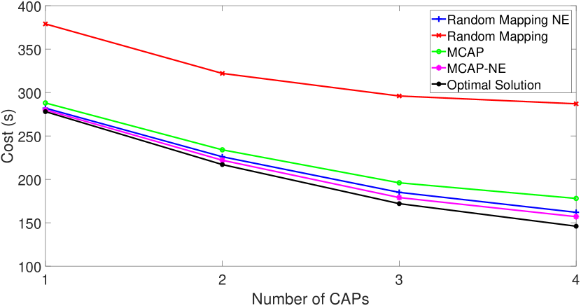
(a) Cost against number of CAPs.

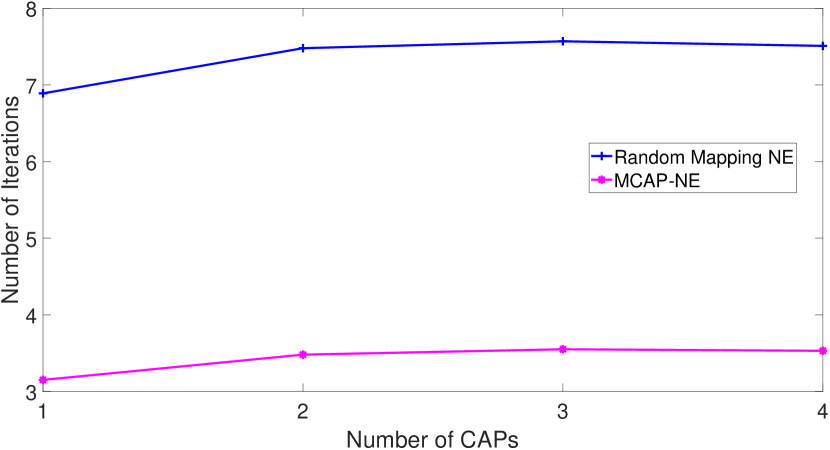
(b) Number of Iterations required against CAPs.

Figure 2: Impact of the Number of CAPs.

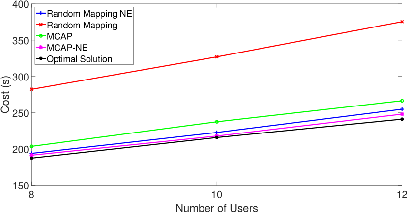
(a) Impact of the number of Users.

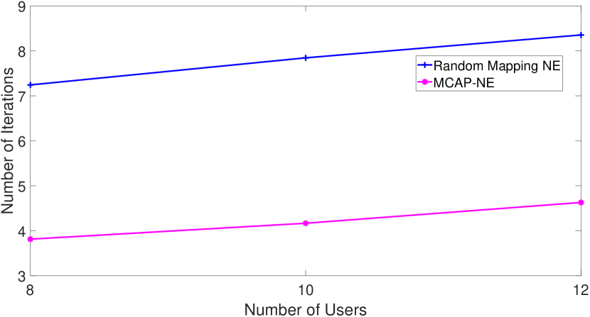
(b) Number of Iterations against the number of Users.

Figure 3: Impact of Number of Users.

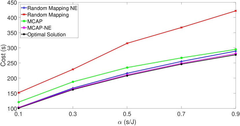
(a) Cost against $\alpha$

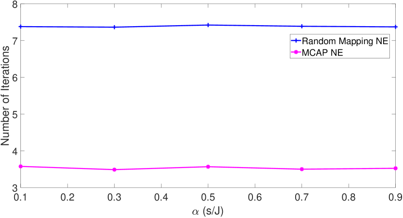
(b) Number of Iterations against $\alpha$.

Figure 4: Impact of $\alpha$.

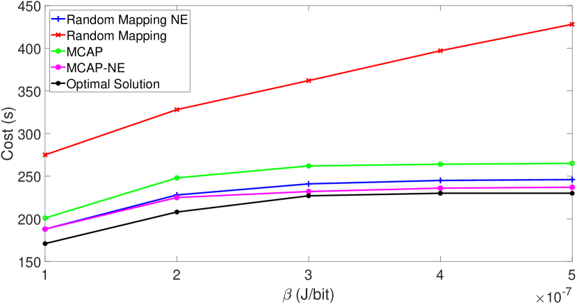
(a) Cost against $\beta$

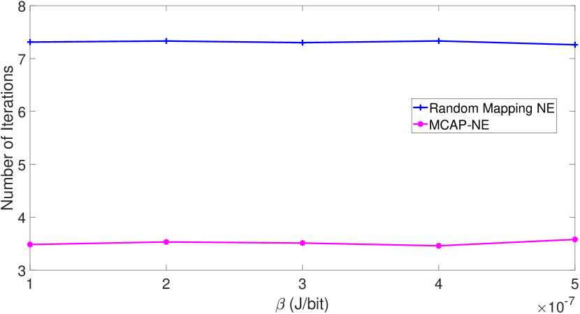
(b) Number of Iterations required $\beta$.

Figure 5: Impact of $\beta$.

Figures 2(b), 3(b), 4(b), and 5(b) show the number of iterations required to compute the NE against the number of CAPs, the number of users, $\alpha$, and $\beta$, respectively, with either a random starting point or an MCAP starting point. In all of these figures, we see that number of iterations required to obtain the NE is more than doubled when using a random starting point as opposed to the MCAP-NE, confirming the performance benefit of using MCAP for an initial starting point. While the addition of CAPs does not noticeably increase the number of iterations required, the number of users does have a discernible effect due to the additional number of possible users who may find an improvement. As expected, $\alpha$ and $\beta$ have no discernible effect as those parameters do not affect the size of the strategy space.

VI-C Placement Constraints

We now study a system in the presence of placement constraints. Here, we consider a system of 12 users by default, randomly assigning as a placement constraint either one of the CAPs or the empty set with equal probability. All of the other parameters of the system are the same as in Section 6.1.

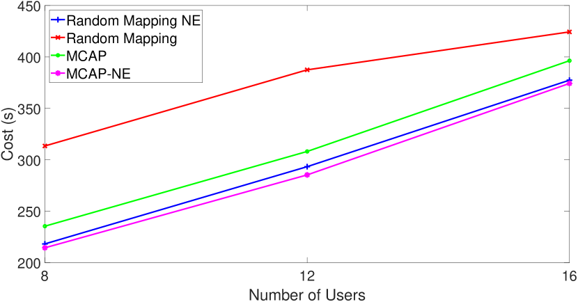
Figure 6: Cost against the number of users with placement constraints

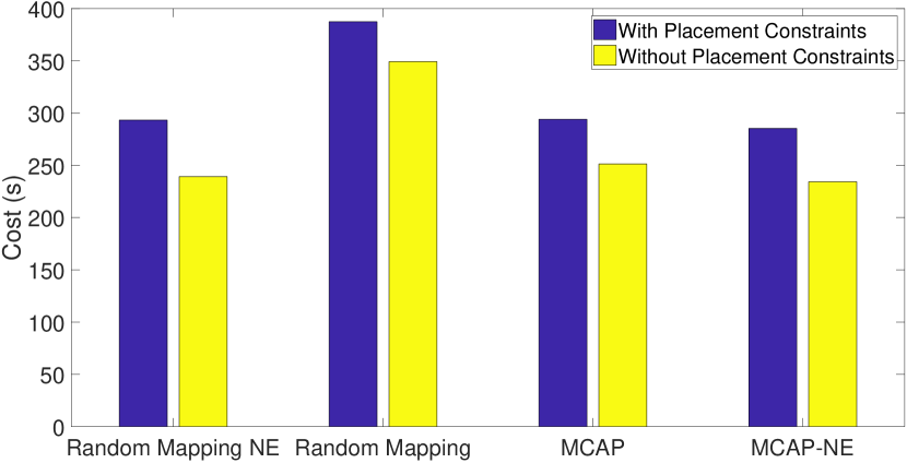
Figure 7: Cost with placement constraints and without placement constraints.

Figures 6 shows the system cost against the number of users under the system with placement constraints. We note that the behaviour here is similar to the behaviour in the system without placement constraints — the cost is increasing with respect to the number of users, and relative performance between offloading methods remain close to the original case. Figure 7 compares a system with placement constraints with a system without placement constraints. We observe that the system with placement constraints requires a higher cost, as beneficial offloading decisions that would otherwise be desirable cannot be made.

VII Conclusion

A multi-user mobile cloud computing system with multiple CAPs has been considered, in which each mobile user has a task to be processed either locally, at one of the CAPs, subject to the user’s placement constraint, or at a remote cloud. We solve the non-convex optimization problem through two approaches: in MCAP we formulate the problem as a QCQP and use an SDP relaxation to arrive at a heuristic solution; while in MCAP-NE, we accommodate selfish users by leveraging the finite improvement property of anordinal potential game to find an NE. Simulation results show near optimal performance of our methods as well as the utility of the SDP starting point in substantially reducing the number of iterations required to compute the NE.

References

• [1] M.-H. Chen, M. Dong, and B. Liang, “Multi-user mobile cloud offloading game with computing access point,” in Proc. IEEE International Conference on Cloud Networking (CLOUDNET), Oct. 2016.
• [2] K. Kumar, J. Liu, Y.-H. Lu, and B. Bhargava, “A survey of computation offloading for mobile systems,” Mobile Networks and Applications, vol. 18, no. 1, pp. 129–140, Feb. 2013.
• [3] “Amazon EC2,” https://aws.amazon.com/ec2/, [Online; accessed 05-2019].
• [4] Y. Mao, C. You, J. Zhang, K. Huang, and K. B. Letaief, “A survey on mobile edge computing: The communication perspective,” IEEE Commun. Surveys Tuts., vol. 19, no. 4, pp. 2322–2358, Aug. 2017.
• [5] B. Liang, “Mobile edge computing,” in Key Technologies for 5G Wireless Systems, V. Wong, R. Schober, D. Ng, and L. Wang, Eds.   Cambridge University Press, 2017.
• [6] ETSI Group Specification, “Mobile edge computing (MEC); framework and reference architecture,” ETSI GS MEC 003 V1.1.1, Mar. 2016.
• [7] A. Greenberg, J. Hamilton, D. A. Maltz, and P. Patel, “The cost of a cloud: Research problems in data center networks,” ACM SIGCOMM Computer Communication Review, vol. 39, no. 1, pp. 68–73, Dec. 2008.
• [8] M. Satyanarayanan, P. Bahl, R. Caceres, and N. Davies, “The case for vm-based cloudlets in mobile computing,” IEEE Pervasive Computing, vol. 8, no. 4, pp. 14–23, Oct. 2009.
• [9] F. Bonomi, R. Milito, J. Zhu, and S. Addepalli, “Fog computing and its role in the internet of things,” in Proc. ACM SIGCOMM Workship on Mobile Cloud Computing, Aug. 2012, pp. 13–16.
• [10] M.-H. Chen, M. Dong, and B. Liang, “Joint offloading decision and resource allocation for mobile cloud with computing access point,” in Proc. IEEE International Conference on Acoustics, Speech and Signal Processing (ICASSP), Mar. 2016, pp. 3516–3520.
• [11] M.-H. Chen, B. Liang, and M. Dong, “Resource sharing of a computing access point for multi-user mobile cloud offloading with delay constraints,” IEEE Transactions on Mobile Computing, vol. 17, no. 12, pp. 2868–2881, Mar. 2018.
• [12] ——, “Joint offloading and resource allocation for computation and communication in mobile cloud with computing access point,” in Proc. IEEE Conference on Computer Communications (INFOCOM), May 2017.
• [13] ——, “Multi-user multi-task offloading and resource allocation in mobile cloud systems,” IEEE Transactions on Wireless Communications, vol. 17, no. 10, pp. 6790–6805, Oct. 2018.
• [14] Z.-Q. Luo, W.-K. Ma, A.-C. So, Y. Ye, and S. Zhang, “Semidefinite relaxation of quadratic optimization problems,” IEEE Signal Processing Magazine, vol. 27, pp. 20–34, 2010.
• [15] D. Monderer and L. S. Shapley, “Potential games,” Games and Economic Behavior, vol. 14, no. 1, pp. 124–143, Jun. 1996.
• [16] W. Zhang, Y. Wen, K. Guan, D. Kilper, H. Luo, and D. Wu, “Energy-optimal mobile cloud computing under stochastic wireless channel,” IEEE Transactions on Wireless Communications, vol. 12, no. 9, pp. 4569–4581, Sep. 2013.
• [17] S. Barbarossa, S. Sardellitti, and P. Di Lorenzo, “Computation offloading for mobile cloud computing based on wide cross-layer optimization,” in Proc. Future Network and Mobile Summit, Jul. 2013.
• [18] W. Zhang, Y. Wen, and D. O. Wu, “Energy-efficient scheduling policy for collaborative execution in mobile cloud computing,” in Proc. IEEE International Conference on Computer Communications (INFOCOM), Apr. 2013.
• [19] M.-H. Chen, B. Liang, and M. Dong, “Joint offloading decision and resource allocation for multi-user multi-task mobile cloud,” in Proc. IEEE International Conference on Communications (ICC), May 2016.
• [20] O. Munoz, A. Pascual-Iserte, and J. Vidal, “Optimization of radio and computational resources for energy efficiency in latency-constrained application offloading,” IEEE Transactions on Vehicular Technology, vol. 64, no. 10, pp. 4738–4755, Nov. 2014.
• [21] R. M. R., N. Venkatasubramanian, S. Mehrotra, and A. V. Vasilakos, “Mapcloud: Mobile applications on an elastic and scalable 2-tier cloud architecture,” in Proc. IEEE/ACM International Conference on Utility and Cloud Computing, Nov. 2012.
• [22] R. M. R., N. Venkatasubramanian, and A. V. Vasilakos, ““music: Mobility-aware optimal service allocation in mobile cloud computing,” in Proc. IEEE International Conference on Cloud Computing, Jun. 2013.
• [23] J. Song, Y. Cui, M. Li, J. Qiu, and R. Buyya, ““energy-traffic tradeoff cooperative offloading for mobile cloud computing,” in Proc. IEEE International Symposium of Quality of Servous (IWQoS), May 2014.
• [24] V. Cardellini, V. D. N. Persone, V. D. Valerio, F. Facchinei, V. Grassi, F. L. Pressit, and V. Piccialli, “A game-theoretic approach to computation offloading in mobile cloud computing,” Mathematical Programming, pp. 1–29, Apr. 2015.
• [25] Y. Wang, X. Lin, and M. Pedram, “A nested two stage game-based optimization framework in mobile cloud computing system,” in Proc. IEEE International Symposium on Service Oriented System Engineering (SOSE), Mar. 2013.
• [26] S. Josilo and G. Dan, “A game theoretic analysis of selfish mobile computation offloading,” in Proc. IEEE Conference on Computer Communications (INFOCOM), May 2017.
• [27] E. Meskar, T. Todd, D. Zhao, and G. Karakostas, “Energy efficient offloading for competing users on a shared communication channel,” in Proc. IEEE International Conference on Communications (ICC), Jun. 2015.
• [28] X. Ma, C. Lin, X. Xiang, and C. Chen, “Game-theoretic analysis of computation offloading for cloudlet-based mobile cloud computing,” in Proc. of ACM MSWiM, Nov. 2015.
• [29] X. Chen, “Decentralized computation offloading game for mobile cloud computing,” IEEE Transactions on Parallel and Distributed Systems, vol. 26, no. 4, pp. 974–983, Apr. 2015.
• [30] X. Chen, L. Jiao, W. Li, and X. Fu, “Efficient multi-user computation offloading for mobile-edge cloud computing,” IEEE/ACM Transactions on Networking, vol. 24, no. 5, pp. 2795–2808, Oct. 2015.
• [31] S. Josilo and G. Dan, “Wireless and computing resource allocation for selfish computation offloading in edge computing,” in Proc. IEEE Conference on Computer Communications (INFOCOM), Apr. 2019.
• [32] H. Cao and J. Cai, “Distributed multi-user computation offloading for cloudlet based mobile cloud computing: A game-theoretic machine learning approach,” IEEE Transactions on Vehicular Technology, vol. 67, no. 1, pp. 752–764, Aug. 2017.
• [33] M. J. Osborne and A. Rubinstein, A Course in Game Theory.   The MIT press, 1994.
• [34] A. P. Miettinen and J. K. Nurminen, “Energy efficiency of mobile clients in cloud computing,” in Proc. USENIX Conference on Hot Topics in Cloud Computing (HotCloud), Jun. 2010.
• [35] ubergizmo.com, “Apple iphone x specifications,” 2017, accessed 2019-07-31. [Online]. Available: https://www.ubergizmo.com/products/lang/en_us/devices/iphone-x/