NT@UW-20-09
The Mystery of Bloom-Gilman Duality: A Light Front Holographic QCD Perspective

Abstract

Light front wave functions motivated by holographic constructions are used to study $\rm Bloom-Gilman\,duality$, a feature of deep inelastic scattering. Separate expressions for structure functions in terms of quark and hadronic degrees of freedom (involving transition form factors) are presented, with an ultimate goal of obtaining a relationship between the two expressions. A specific two-parton model is defined and resonance transition form factors are computed using previously derived light front wave functions. A new form of global duality (integral over all values of $x$ between 0 and 1) is derived from the valence quark-number sum rule. Using a complete set of hadronic states is necessary for this new global duality to be achieved, and the previous original work does not provide such a set. This feature is remedied by amending the model to include a longitudinal confining potential, and the resulting complete set is sufficient to carry out the study of $\rm Bloom-Gilman\,duality$. Specific expressions for transition form factors are obtained and all are shown to fall as $1/Q^{2}$, at asymptotically large values. This is because the Feynman mechanism dominates the asymptotic behavior of the model. These transition form factors are used to assess the validity of the global and local duality sum rules, with the result that both are not satisfied within the given model. Evaluations of the hadronic expression for $q(x,Q^{2})$ provide more details about this lack. This result is not a failure of the current model because it shows that the observed validity of both global and local forms of duality for deep inelastic scattering must be related to a feature of QCD that is deeper than completeness. Our simple present model suggests a prediction that $\rm Bloom-Gilman\,duality$ would not be observed if deep inelastic scattering experiments were to be made on the pion. The underlying origin of the duality phenomenon in deep inelastic scattering is deeply buried within the confinement aspects of QCD, and its origin remains a mystery.

I Introduction

Two distinct facets of QCD are known. At asymptotically high-energies and momentum transfers $Q^{2}$ many hadronic observables can be computed using quarks and gluons as degrees of freedom and applying perturbation theory. At low-momentum scales the theory is strongly coupled so that hadronic degrees of freedom and non-perturbative methods must be used. It has therefore been very surprising that examples in which the behavior of low-$Q^{2}$ cross sections can be related, through suitable averaging procedures to those at high $Q^{2}$ actually exist. This phenomenon became known as quark-hadron duality. See the review Melnitchouk et al. (2005).

Here we focus on deep-inelastic scattering from hadrons. Bloom and Gilman Bloom and Gilman (1970, 1971) studied data from the early DIS experiments at SLAC. They found that the inclusive structure function measured at low values of the hadronic final state mass, $W$, generally follows a curve that describes data at large values of $W$. In particular average values of the low $W$ cross sections were found to be approximately equal to that of the high $W$ cross section, which approximately obeys Bjorken scaling. Moreover, averages of low $Q^{2}$ data over specific kinematic regions were found to be equal to the high $W$ cross section.

Bloom-Gilman duality was later examined in terms of an operator product expansion of moments of structure functions De Rujula et al. (1976, 1977). This work found a systematic classification of terms responsible for duality, but did not describe how the physics of resonances transforms into the physics of scaling. The subject of Bloom-Gilman duality was largely ignored for about 20 years.

The availability of high-luminosity beams of electrons at Jefferson Laboratory allowed the subject to be studied in great detail. A striking finding was that Bloom-Gilman duality appears to work at values of $Q^{2}$ as low as about 1 GeV² or less Niculescu et al. (2000a, b); Ent et al. (2000).

Finding an elementary understanding of the origins of Bloom-Gilman duality has been elusive because it involves trying to build up structure function that is independent of $Q^{2}$ (except for the logarithmic corrections of QCD) entirely out of resonances, each of which is described by a form factor that falls rapidly with $Q^{2}$.

The description of Bjorken scaling in deep inelastic (DIS) structure functions is most simply formulated in terms of the quark-parton model, which is well understood in terms of a twist expansion, but the physical final state is composed of hadrons. The validity of both approaches indicates that describing DIS in terms of hadronic degrees of freedom should be possible. One of the central mysteries of strong-interaction physics is how scattering from confined bound states of quarks and gluons can be consistent with Bjorken scaling, a property associated with free quarks.

Previous approaches to understanding the origins of $\rm Bloom-Gilman\,duality$, reviewed in Melnitchouk et al. (2005), include QCD in 1 +1 dimensions Einhorn (1976), phenomenological approaches Domokos et al. (1971a, b) harmonic oscillator models Isgur et al. (2001); Jeschonnek and Van Orden (2004); Close and Zhao (2002); Harrington (2002) and other models  Close and Isgur (2001); Paris and Pandharipande (2001, 2002). Non-relativistic potential models can describe or represent confining systems with an infinite number of bound states, thereby indicating how it is that Bloom-Gilman scaling may arise, but are not properly relativistic. This means that none obtain Lorentz invariant quark distributions that have the correct support properties of being non-zero only in the region where Bjorken $x$ varies between 0 and 1. Understanding $\rm Bloom-Gilman\,duality$ requires models that are both confining and relativistic.

We aim to understand $\rm Bloom-Gilman\,duality$ by using relativistic light-front wave functions obtained from light front holographic QCD, an approach defined in the review Brodsky et al. (2015), that provides a relativistic treatment of confined systems. We briefly summarize following Ref. Brodsky et al. (2015). Light-front quantization is a relativistic, frame independent approach to describing the constituent structure of hadrons. The simple structure of the light-front (LF) vacuum allows an unambiguous definition of the partonic content of a hadron in QCD and of hadronic light-front wave functions, the underlying link between large distance hadronic states and the constituent degrees of freedom at short distances. The QCD light-front Hamiltonian $H_{LF}$ is constructed from the QCD Lagrangian using the standard methods of quantum field theory Brodsky et al. (1998). The spectrum and light-front wave functions of relativistic bound states are obtained from the eigenvalue equation $H_{LF}|\psi\rangle=M^{2}|\psi\rangle$. It becomes an infinite set of coupled integral equations for the LF components in a complete basis of non-interacting $n$-particle states, with an infinite number of components. This provides a quantum-mechanical probabilistic interpretation of the structure of hadronic states in terms of their constituents at the same light-front time $x^{+}=x^{0}+x^{3}$, the time marked by the front of a light wave Dirac (1949). The Hamiltonian eigenvalue equation in the light front is frame independent. The matrix diagonalization Brodsky et al. (1998) of the LF Hamiltonian eigenvalue equation in four-dimensional space-time has not yet been achieved because various technical and difficulties and because of a lack of understanding of the fundamental mechanism of confinement. Therefore other methods and approximations are needed to truly understand the nature of relativistic bound states in the strong-coupling regime of QCD.

To a first semiclassical approximation, where quantum loops and quark masses are not included, the relativistic bound-state equation for light hadrons can be reduced to an effective LF Schrödinger equation. The technique is to identify the invariant mass of the constituents as a key dynamical variable. The invariant mass measures the off-shellness in the LF kinetic energy, so that it is the natural variable to characterize the hadronic wave function. In conjugate position space, the relevant dynamical variable is an invariant impact kinematical variable $\zeta$, which measures the separation of the partons within the hadron at equal light-front time de Teramond and Brodsky (2009). Thus, the multi-parton problem in QCD is reduced, in a first semi-classical approximation, to an effective one dimensional quantum field theory by properly identifying the key dynamical variable. As a result, complexities of the strong interaction dynamics are hidden in an effective potential $U(\zeta)$, but the central question – how to derive the confining potential from QCD, remains open.

It is remarkable that in the semiclassical approximation described above, the light-front Hamiltonian has a structure which matches exactly the eigenvalue equations in AdS space Brodsky et al. (2015). This offers the possibility to explicitly connect the AdS wave function $\Phi(z)$ to the internal constituent structure of hadrons. In fact, one can obtain the AdS wave equations by starting from the semiclassical approximation to light-front QCD in physical space-time. This connection yields a relation between the coordinate $z$ of AdS space with the impact LF variable $\zeta$ de Teramond and Brodsky (2009), thus giving the holographic variable $z$ a precise definition and intuitive meaning in light-front QCD.

Light-front holographic methods were originally introduced Brodsky and de Teramond (2006, 2008a) by matching the electromagnetic current matrix elements in AdS space Polchinski and Strassler (2003) with the corresponding expression derived from light-front quantization in physical space-time Drell and Yan (1970a); West (1970). It was also shown that one obtains identical holographic mapping using the matrix elements of the energy-momentum tensor Brodsky and de Teramond (2008b) by perturbing the AdS metric around its static solution Abidin and Carlson (2008), thus establishing a precise relation between wave functions in AdS space and the light-front wave functions describing the internal structure of hadrons.

The light front wave functions that arise out of this light front holographic approach provide a new way to study old problems that require the use of relativistic-confining quark models. The study of $\rm Bloom-Gilman\,duality$ is an excellent example of such a problem.

The present treatment is outlined next. Sect. II is concerned with general definitions related to DIS for spin-less targets. Separate expressions for structure functions using both quark and hadronic degrees of freedom are presented, with the fundamental aim of the paper to relate the two. The global and local forms of $\rm Bloom-Gilman\,duality$ are reviewed briefly in Sect. III. The next Section, IV, is concerned with presenting the main features of light-front wave functions for two-parton systems that are obtained from the $z-\zeta$ connection. The valence quark number sum rule is discussed as a new global duality in Sect. V. This relation is satisfied in models that provide a complete set of wave functions. The existing light front wave functions, summarized in Ref. Brodsky et al. (2015), are found to be incomplete in Sect. VI. This is because excitations in the longitudinal degree of freedom are not incorporated. Completeness is implemented by including a longitudinal confining potential in Sect. VII. Evaluations of transition form factors are presented in Sec. VIII. The two-parton model is shown to violate both the global and local forms of $\rm Bloom-Gilman\,duality$ in Secs. IX and X. The model’s quark distributions are evaluated in Sec. XI. The results are summarized and discussed in Sec. XII.

II Deep Inelastic Scattering From a spin zero target -General Preliminaries

The hadronic tensor for a spin-less or spin-averaged target is given by

$$W^{\mu\nu}=(p^{\mu}-{p\cdot q\,q^{\mu}\over q^{2}})(p^{\nu}-{p\cdot q\,q^{\nu}\over q^{2}}){W_{2}\over M^{2}}+(g^{\mu\nu}-{q^{\mu}q^{\nu}\over q^{2}})W_{1},$$ (1)

with $p$ as the target four-momentum ($p^{2}=M^{2}$) and $q$ that of the virtual photon. The quantity $W^{\mu\nu}$ is the matrix element of a current-current correlation function:

$$W^{\mu\nu}={1\over 4\pi}\int d^{4}\xi e^{iq\cdot\xi}\langle p|j^{\mu}(\xi)j^{\nu}(0)|p\rangle,$$ (2)

with normalization $\langle p^{\prime}|p\rangle=2p^{+}\delta(p^{+}-{p^{\prime}}^{+})(2\pi)^{3}\delta({\bf p}-{\bf p}^{\prime})$. At large values of $Q^{2}$, the correlation is along the light cone. For space-like four momenta $q^{\mu}$ one may choose the $z$ axis such that $q^{+}=0$, for space-like values of $q^{\mu}$, This enables the use of the Drell-Yan formula Drell and Yan (1970b) for form factors. With this notation $q^{3}=-\nu$ , $|{\bf q}|=Q,\ {\bf q}^{2}=Q^{2},\,\vec{q}\,^{2}=\nu^{2}+Q^{2}$. Here bold-face indicates transverse vectors and $\vec{q}$ is the three-dimensional vector.

II.1 Quark Degrees of Freedom

The expression Eq. (2) can be handled by turning the product of currents into a commutator and then making the operator product expansion. The resulting leading-twist contribution to the quark distribution for a quark, $q(x)$ is given by

$$q(x)=\int{dx^{-}\over 4\pi}e^{ixP^{+}x^{-}}\langle p|\bar{\psi}(-x^{-}/2)\gamma^{+}\psi(x^{-}/2)|p\rangle,$$ (3)

where $\psi$ is a quark-field operator, the notation $x^{-}/2$ refers to $x^{\mu}=(0,-x^{-}/2,{\bf 0})$, and $x=Q^{2}/2p\cdot q$. Scale dependence due to QCD evolution is omitted in this paper. Eq. (3) is understood as involving wave functions evaluated at a given momentum scale. Thus the structure functions discussed reflect the intrinsic bound-state structure of the hadrons, and thus apply only at low resolution scales. Bloom & Gilman did not consider QCD evolution in their work. Accordingly such effect are not a part of the present initial modern analysis.

One extracts $W_{2}$ from $W^{\mu\nu}$ by using

$$W_{2}=W^{++}.$$ (4)

At leading twist

$$W_{2}=2M^{2}{x\over p\cdot q}W_{1},$$ (5)

where $M$ is the ground state mass.

II.2 Hadronic Degrees of Freedom

An expression for $W^{++}$ can be obtaining using hadrons by inserting a complete set of hadronic states $|X\rangle$ between the current operators in Eq. (2). The use of $\langle p|j^{\mu}(\xi)|X\rangle=e^{i(p-p_{X})\cdot\xi}\langle p|j^{\mu}(0)|X\rangle$, taking $\mu=+,\nu=+$ and integrating over $\xi^{+}$ yields

$$W^{++}=\sum_{X}{1\over 2E_{X}}\delta(p^{-}+q^{-}-p_{X}^{-})|\langle X,x|j^{+}(0)|p\rangle|^{2},$$ (6)

in which it is understood that $\vec{p}_{X}=\vec{p}+\vec{q}=\vec{q}$, in the lab frame. The notation $X,x$ is meant to include all degenerate states of the same angular momentum. The factor of $2E_{X}$ in the denominator comes from the relativistic normalization of states. The matrix elements of $j^{+}(0)$ are proportional to form factors:

$$|F_{X,0}|^{2}\equiv\sum_{x}|\langle X,x|{j^{+}(0)\over 2p^{+}}|p\rangle|^{2},$$ (7)

with $p_{X}^{+}=p^{+}+q^{+}=p^{+}$. The matrix element involves only internal coordinates of the wave functions, and 0 denotes the ground state in the lab frame with $\vec{p}=0$.

The argument of the delta function appearing in Eq. (6) can be expressed in more detail as

$$p^{-}+q^{-}-p_{X}^{-}=M+\nu-E_{X}(\vec{q})=E_{0}+\nu-\sqrt{M_{X}^{2}+Q^{2}+\nu^{2}},$$ (8)

where $M$ is the ground state energy Then using $W^{++}=W_{2}$, we find

$$W_{2}=4M^{2}\sum_{X}{1\over 2\sqrt{M_{X}^{2}+Q^{2}+\nu^{2}}}\delta(M+\nu-\sqrt{M_{X}^{2}+Q^{2}+\nu^{2}})|F_{X}|^{2}.$$ (9)

$$=4M^{2}\sum_{X}\delta\bigg{(}M^{2}-M_{X}^{2}+Q^{2}({1\over x}-1)\bigg{)}|F_{X}|^{2}.$$ (10)

The study of Bloom-Gilman duality involves relating the quark Eq. (3) and hadronic expressions Eq. (10).

III Bloom-Gilman Duality

Bloom and Gilman found that the structure function in the resonance region, $W<2$ GeV, was roughly equivalent on average to the scaling one, with averages obtained over the same region of the scaling variable:

$$\omega^{\prime}={2M\nu+M^{2}\over Q^{2}}=1+{W^{2}\over Q^{2}}={1\over x}+{M^{2}\over Q^{2}},$$ (11)

where the invariant energy, $W$, is given by $W^{2}=(p+q)^{2}=M^{2}+2M\nu-Q^{2},$ which is the square of the mass of a resonance that is excited. Application of Eq. (11) requires that $\omega^{\prime}>0$ and $x>0$, so that $Q^{2}>M^{2}$. Bloom & Gilman noted that their sum rule is not valid if $Q^{2}$ is much less than 1 GeV².

Bloom and Gilman found that the data from the resonance region at low $Q^{2}$ oscillate around the scaling curve, with averages that are equal to the scaling curve. Furthermore the resonances move to lower values of $\omega^{\prime}$ (higher values of $x$) with increasing $Q^{2}$. These observations were repeated at Jefferson Lab.

Bloom and Gilman quantified their studies by observing the validity of a sum rule:

$${2M\over Q^{2}}\int_{0}^{\nu_{m}}d\nu\,\nu W_{2}(\nu,Q^{2})=\int_{1}^{1+W_{m}^{2}/Q^{2}}d\omega^{\prime}\nu W_{2}(\omega^{\prime}),$$ (12)

where $W_{2}(\omega^{\prime})$ is scaling function obtained at large values of $Q^{2}$. The upper limit on the integration over $\nu$, $\nu_{m}=(W_{m}^{2}-M^{2}+Q^{2})/2M$ corresponds to the maximum value of $\omega^{\prime}=1+W_{m}^{2}/Q^{2}$, where $W_{m}\approx 2$ GeV. The validity of this equation is known as global duality.

Local duality is said to exist if the equality of the averaged resonance and scaling functions holds over restricted regions of $W$. BG obtained an explicit expression by taking the difference between two versions of Eq. (12) with different upper limits of integration.

$${2M\over Q^{2}}\int_{\nu_{a}}^{\nu_{b}}d\nu\,\nu W_{2}(\nu,Q^{2})=\int_{1+W_{b}^{2}/Q^{2}}^{1+W_{a}^{2}/Q^{2}}d\omega^{\prime}\nu W_{2}(\omega^{\prime}).$$ (13)

IV Soft-wall Light Front Wave Functions in Light Front Holographic QCD

Consider a hadronic bound state of two constituents, each of vanishing mass. We follow the argument of Brodsky et al. (2015). The eigenmasses are given by

$$M^{2}=\int_{0}^{1}\int\psi^{*}(x,\mathbf{k})\bigg{[}\dfrac{-\nabla^{2}_{\mathbf{k}}}{x(1-x)}\bigg{]}\psi(x,\mathbf{k})dx\ {d^{2}\mathbf{k}\over 16\pi^{3}}+\text{interactions},$$

$$=\int_{0}^{1}\int\psi^{*}(x,\mathbf{b})\bigg{[}\dfrac{-\nabla^{2}_{\mathbf{b}}}{x(1-x)}\bigg{]}\psi(x,\mathbf{b})dx\ {d^{2}\mathbf{b}\over 4\pi}+\text{interactions}$$ (14)

where the relative coordinates are the transverse separation ${\bf b}$ and the momentum fraction $x$. The invariant mass $M_{q\bar{q}}^{2}={{\bf k}^{2}\over x(1-x)}$. The canonically conjugate impact space variable is $\zeta^{2}=x(1-x){\bf b}^{2}$. To a first approximation light front (LF) dynamics depend only on $M_{q\bar{q}}^{2}$ or $\zeta$, and the dynamical properties are encoded in the hadronic wave function $\phi(\zeta)$. Following standard procedures solutions in the product form,

$$\psi(x,\zeta,\phi)=e^{iL_{z}\varphi}X(x){\phi(\zeta)\over\sqrt{2\pi\zeta}},$$ (15)

are sought. The quantity $L_{z}$ is the longitudinal component of the orbital angular momentum, an integer that can be positive of negative or 0.

One proceeds by writing the Laplacian operator in Eq. (14) in the polar coordinates $(\zeta,\phi)$;

$$\nabla_{\zeta}^{2}={1\over\zeta}{d\over d\zeta}\big{(}\zeta{d\over d\zeta}\big{)}+{1\over\zeta^{2}}{\partial^{2}\over\partial\varphi^{2}}$$ (16)

Then with the normalization

$$\langle X|X\rangle=\int_{0}^{1}{dx\over x(1-x)}X^{2}(x)=1$$ (17)

one finds that Eq. (14) becomes

$$M^{2}=\int d\zeta\phi^{*}(\zeta)\bigg{(}-{d^{2}\over d\zeta^{2}}-{1-4L^{2}\over 4\zeta^{2}}\bigg{)}\phi(\zeta)+\int d\zeta\phi^{*}(\zeta)U(\zeta)\phi(\zeta)$$ (18)

in which an effective potential $U(\zeta)$ has been introduced to enforce confinement at some infrared scale, and $L$ is the absolute value of $L_{z}$.

The resulting wave equation is

$$\bigg{(}-{d^{2}\over d\zeta^{2}}-{1-4L^{2}\over 4\zeta^{2}}+U(\zeta)\bigg{)}\phi(\zeta)=M^{2}\phi(\zeta)$$ (19)

The soft-wall model  Karch et al. (2006)

$$U(\zeta)=\kappa^{4}\zeta^{2}$$ (20)

where $\kappa$ is the strength of the confinement, is used here. This form was used in  de Téramond and Brodsky (2009). Later work de Téramond et al. (2015); Dosch et al. (2015) introduced a constant term that depends on $L$, and relations between the baryon and meson spectrum was obtained. These results were derived from super-conformal algebra. In line with our goal of examining Bloom-Gilman duality, the earlier form is used here to avoid a zero in the ground state mass.

The function $X(x)$ is to be determined. A popular choice has been to simply use $X(x)=\sqrt{x(1-x)}.$ This is followed here. We’ll show below that this choice does not yield a complete set of wave functions in three-dimensional space.

The associated eigenvalues are :

$$M^{2}_{nL}=\kappa^{2}(4n+2L+2).$$ (21)

The light-front wave function (Eq. (15)) is obtained by solving Eq. (19) with the soft-wall potential of Eq. (20), and using $\zeta^{2}=x(1-x)b^{2}$ with the result:

$$\psi_{nL_{z}}({\bf b},x)=A_{nL}\sqrt{x(1-x)}{e^{iL_{z}\varphi}\over\sqrt{2\pi}}e^{-\kappa^{2}b^{2}x(1-x)/2}(\sqrt{x(1-x)}b)^{L}L_{n}^{L}(\kappa^{2}b^{2}x(1-x)).$$ (22)

where $b$ is the transverse radius, $\varphi$ is the transverse angle, and $x$ is the plus-momentum ratio of one of the quarks. The factor normalizing the wave function to unity is: $A_{nL}={\sqrt{2}}\sqrt{n!\over(n+L)!}.$ The spin-dependence is taken be a simple delta function, setting the helicity of the anti-quark to the negative of the quark Lepage and Brodsky (1980); Brodsky and de Teramond (2008a). The action of the $\gamma^{+}$ operator in $j^{+}$ conserves the spin of the struck quark so that all of the states, $X$ entering in Eq. (10) have the same spin wave function.

The next step is to evaluate the transition form factors. For a quark-anti-quark system, of unit charge, with the given space and spin dependence, in the Drell-Yan frame, these are given by the expression:

$$F_{X0}({\bf q})\equiv F_{nL_{z}}({\bf q})=\int_{0}^{1}dx\int d^{2}{\bf b}\ \ \ e^{i{{\bf q}}\cdot{{\bf b}}(1-x)}\ \psi^{*}_{nL_{z}}(x,{{\bf b}})\ \psi_{00}(x,{\bf b}),$$ (23)

with the notation $({\bf q}\cdot{\bf q}=Q^{2})$. This form factor is the same as would be obtained if only a single quark of unit charge interacts electromagnetically.

V Valence Quark number sum Rule- a New Global Duality

In this two-parton model the quark and anti-quark have the same relative wave function and therefore the same quark distribution. The form factor can be obtained as if only a single quark of unit charge interacts electromagnetically. In this case the form factors of Eq. (7) contribute to the single flavor $q(x,Q^{2})$. This means that the sum over $X$ in Eq. (10) contributes only to $q(x)$, and we may take the quark distribution $q(x)$ as given by

$$q(x)=W_{1}={p\cdot q\over 2M^{2}x}W_{2}={\nu\over 2Mx}W_{2}.$$ (24)

An interesting sum rule may be derived from the valence quark number sum rule:

$$\int_{0}^{1}q(x)dx=1.$$ (25)

The integral over $x$ can be evaluated from the hadronic degrees of freedom, using Eq. (24) and Eq. (10) we examine the quark number sum rule to find

$$q(x,Q^{2})={Q^{2}\over x^{2}}\sum_{X}\delta\bigg{(}M^{2}-M_{X}^{2}+Q^{2}({1\over x}-1)\bigg{)}|F_{X}|^{2}$$ (26)

Noting that $F_{X}$ depends on $Q^{2}$, not on $x$, the integral over all values of $x$ yields

$$\int_{0}^{1}q(x)dx=\sum_{X}|F_{X}|^{2}.$$ (27)

Thus the quark number sum rule is satisfied if and only if the completeness relation

$$\sum_{X}|F_{X}|^{2}=1$$ (28)

is satisfied.

This result Eq. (27) amounts to a new form of global duality: At any given value of $Q^{2}$ the sum of the squares of all of the form factors, computed using hadron degrees of freedom, satisfies the quark number sum rule. The derivation presented here uses a single quark flavor and unit quark charge. The same global duality may be obtained in terms of the usual more general parton model conditions. It is a consequence of baryon number conservation.

VI Lack of Completeness

In the current model the sum appearing in Eq. (28) is given by

$$S(Q)=\sum_{n=0}^{\infty}\sum_{L_{z}=-\infty}^{\infty}\bigg{|}F_{nL_{z}}(Q)\bigg{|}^{2},$$ (29)

Satisfying the sum rule requires $S(Q)=1$.

Let’s evaluate this quantity. To see this more explicitly consider

$$S(Q)\equiv\sum_{n=0}^{\infty}\sum_{L_{z}=-\infty}^{\infty}\bigg{|}F_{nL_{z}}(Q)\bigg{|}^{2}$$ (30)

$$=\int dx\int d^{2}be^{i{\bf q}\cdot{\bf b}(1-x)}\psi_{n,L_{z}}^{*}(x,{\bf b})\psi_{00}(x,{\bf b})\int dx^{\prime}\int d^{2}r^{\prime}e^{-i{\bf q}\cdot{\bf b}^{\prime}(1-x^{\prime})}\psi_{n,L_{z}}(x^{\prime},{\bf b}^{\prime})\psi_{00}(x^{\prime},{\bf b}^{\prime})$$ (31)

Change variables to $\mbox{\boldmath$\zeta$}={\bf b}\sqrt{x(1-x)}$. Then use $d^{2}bx(1-x)=d^{2}\zeta$ and define

$$\phi_{nL_{z}}(\mbox{\boldmath$\zeta$})\equiv{\psi_{nL_{z}}(x,\mbox{\boldmath$\zeta$})\over\sqrt{x(1-x)}}.$$ (32)

The $\phi_{nL_{z}}(\mbox{\boldmath$\zeta$})$ are standard two-dimensional harmonic oscillator wave functions. Then

$$S(Q)=\sum_{n=0}^{\infty}\sum_{L_{z}=-\infty}^{\infty}\int dx\int d^{2}\zeta e^{i{\bf q}\cdot\mbox{\boldmath$\zeta$}\sqrt{1-x\over x}}\phi_{n,L_{z}}^{*}(\mbox{\boldmath$\zeta$})\phi_{00}(x,\mbox{\boldmath$\zeta$})\int dx^{\prime}\int d^{2}b^{\prime}e^{-i{\bf q}\cdot\mbox{\boldmath$\zeta$}^{\prime}\sqrt{1-x^{\prime}\over x^{\prime}}}\phi_{n,L_{z}}(\mbox{\boldmath$\zeta$}^{\prime})\phi_{00}(\mbox{\boldmath$\zeta$}^{\prime})$$ (33)

But standard 2D ho wfs obey

$$\sum_{n=0}^{\infty}\sum_{L_{z}=-\infty}^{\infty}\phi_{n,L_{z}}^{*}(\mbox{\boldmath$\zeta$})\phi_{n,L_{z}}(\mbox{\boldmath$\zeta$}^{\prime})=\delta(\mbox{\boldmath$\zeta$}-\mbox{\boldmath$\zeta$}^{\prime}),$$ (34)

so that

$$S(Q)=\int dx\int dx^{\prime}\int d^{2}\zeta e^{i{\bf q}\cdot\mbox{\boldmath$\zeta$}(\sqrt{1-x\over x}-\sqrt{1-x^{\prime}\over x^{\prime}})}|\phi_{00}(\mbox{\boldmath$\zeta$})|^{2}$$ (35)

The integral over $\zeta$ can be done so that

$$S(Q)=\int dx\int dx^{\prime}e^{-1/4Q^{2}(\sqrt{1-x\over x}-\sqrt{1-x^{\prime}\over x^{\prime}})^{2}}$$ (36)

The validity of the sum rule requires that $S(Q)=1$ for all values of $Q$. This is true only for $Q=0$. For all other values, it is manifest that $S(Q>0)<1$. Completeness is not satisfied. Numerical work shows that $\lim_{Q\to\infty}S(Q)\sim{1\over Q},$ and one can analytically show $\lim_{Q\to\infty}S(Q)\approx\frac{\pi^{3/2}}{8Q}$ by using the method of steepest descent. The net result is that instead of unity one gets 0 for large enough values of $Q$.

This study of $S(Q)$ shows that Eq. (29) is NOT satisfied in the current model. This is because the wave function given above in Eq. (22) are complete only in the two-dimensional $\zeta$ space, not in the $x$ space.

VII Implementing completeness

The functions of Eq. (22) do not form a complete set over the three-dimensional space space $x,{\bf r}$ because $X(x)=\sqrt{x(1-x)}$ is not a complete set of wave functions in $x$ space. The need to include excitations of longitudinal modes has noted in Ref. Li et al. (2016).

Here we construct a set of wave functions in $x$ space in which the given $X(x)$ corresponds to a ground state. This is done by generalizing the interaction to include a longitudinal potential

$$U_{\cal L}(x)=-\lambda\kappa^{2}{d\over dx}x(1-x){d\over dx}.$$ (37)

This interaction is approximately harmonic oscillator potential in the longitudinal variable $\tilde{z}$ of Miller and Brodsky (2020), with $\tilde{z}^{2}=-{\partial^{2}\over\partial x^{2}}$. The factor $x(1-x)$ appears here and in the transverse soft-wall potential of Eq. (20) when it is expressed in terms of light-front variables.

This added potential gives a contribution to the square of the mass, $M_{\cal L}^{2}$ given by

$$M^{2}_{\cal L}=-\lambda\kappa^{2}\int_{0}^{1}dx{X(x)\over\sqrt{x(1-x)}}{d\over dx}x(1-x){d\over dx}{X(x)\over\sqrt{x(1-x)}},$$ (38)

where $\lambda$ is a dimensionless number. The normalized solutions to the related differential equation are the functions

$${X(x)\over\sqrt{x(1-x)}}=\sqrt{2{\cal L}+1}P_{\cal L}(2x-1),$$ (39)

where $P_{\cal L}$ is a Legendre polynomial (with ${\cal L}$ an integer) with eigenvalues $M_{\cal L}^{2}=\lambda\kappa^{2}{\cal L}({\cal L}+1)$. For ${\cal L}=0,\,X(x)=\sqrt{x(1-x)}$ so previous results for the spectrum are preserved and correspond to modes with ${\cal L}=0$.

The value of $\lambda$ should be determined by an appropriate symmetry. We hope that the need to satisfy completeness will lead to future work on this topic and leave finding such a symmetry for future work and future workers. Our only purpose here is to study Bloom-Gilman duality. A complete set of states is needed to do that, as shown in Sect. V. Here we note that setting $\lambda=2$ means the low-energy part of the spectrum obtained in Refs. de Téramond et al. (2015); Dosch et al. (2015) is not changed.

The net result is that light-front wave functions that provide the necessary complete set are given by

$$\Psi_{nL_{z}{\cal L}}(x,\varphi,{\bf r})=\psi_{nL_{z}}({\bf r},x)\sqrt{x(1-x)}P_{\cal L}(2x-1)$$ (40)

Using $\Psi_{n,L_{z}{\cal L}}$ satisfies the completeness relation in the $(x,{\bf b})$ space because the Legendre polynomials form a complete set of orthogonal polynomials.

The spectrum is now given by

$$M^{2}_{nL{\cal L}}(\lambda)=\kappa^{2}(4n+2L+2{\cal L}({\cal L}+1)+2).$$ (41)

VIII Transition Form Factors

The transition form factors must be evaluated in preparation for calculating $W_{2}$ as given by the hadronic expression of Eq. (10). Specific expressions for these form factors have not been presented previously.

Let’s start with the ${\cal L}=0$ sector. The angular integral appearing in $d^{2}b$ can be done in closed form with the result:

$$F_{nL_{z}}({\bf q})=(-i)^{L_{z}}{2}\sqrt{n!\over(n+L)!}\int_{0}^{1}dx\int_{0}^{\infty}dz\,z^{L+1}e^{-z^{2}}L_{n}^{L}(z^{2})J_{L}\big{(}Qz\sqrt{1-x\over x}\big{)}$$ (42)

Evaluation leads to

$$F_{nL_{z}}(Q)={(-i)^{L_{z}}}\sqrt{\frac{1}{n!(n+L)!}}\ \int_{0}^{1}dx\ \bigg{(}\frac{Q}{2\kappa}\sqrt{\frac{1-x}{x}}\bigg{)}^{N}e^{-\frac{Q^{2}}{4\kappa^{2}}\frac{1-x}{x}},$$ (43)

in which $|{\bf q}|=Q$ is used and $N\equiv 2n+L$.

This integral is found analytically in terms of an incomplete Gamma function as

$$F_{nL_{z}}(Q)=(-i)^{L_{z}}\ \sqrt{\frac{1}{n!(n+L)!}}\frac{2^{-(N+1)}}{N}\Gamma\Big{(}\frac{N+2}{2}\Big{)}\Bigg{(}-2^{N}\frac{Q^{2}}{\kappa^{2}}\ +\ e^{Q^{2}/4\kappa^{2}}\Big{(}\frac{Q}{\kappa}\Big{)}^{N}\Big{(}\frac{q^{2}}{\kappa^{2}}+2N\Big{)}\ \Gamma\Big{(}\frac{2-N}{2},\frac{Q^{2}}{4\kappa^{2}}\Big{)}\Bigg{)}$$ (44)

An alternate evaluation of the integral that allows the asymptotic limit of the transition form factors to be obtained is given next.

Define

$$I_{N}\equiv\int_{0}^{1}dx\ \bigg{(}\frac{Q}{2\kappa}\sqrt{\frac{1-x}{x}}\bigg{)}^{N}e^{-\frac{Q^{2}}{4\kappa^{2}}\frac{1-x}{x}}$$ (45)

with

$$F_{nL_{z}}(Q)=(-i)^{L_{z}}\ \sqrt{\frac{1}{n!(n+L)!}}I_{N}(Q).$$ (46)

Let $K\equiv N/2$, $z\equiv{Q^{2}\over 4\kappa^{2}}$ and $u\equiv{1-x\over x}$. Then

$$I_{K}(z)=z^{K}\int_{0}^{\infty}{du\over(1+u)^{2}}u^{K}e^{-zu}=z\Gamma(K)\left(e^{z}(K+z)E_{K}(z)-1\right),K>0,$$ (47)

with

$$E_{K}(z)=\int_{1}^{\infty}{e^{-zt}\over t^{K}}dt,$$ (48)

and

$$I_{0}(z)=\int_{0}^{\infty}{du\over(1+u)^{2}}e^{-zu}=1-ze^{z}\int_{z}^{\infty}{e^{-t}\over t}dt$$ (49)

It is useful to consider the asymptotic values of the transition form factors for fixed values of $K$ and $z\gg K$. This is because Bloom & Gilman found that one of the requirements for local duality is that all of the transition form factors have the same dependence on $Q^{2}$. First note that for integer values of $K$ one may write

$$I_{K}(z)=z^{K}(-{\partial\over\partial z})^{K}I_{0}(z).$$ (50)

The asymptotic limit of $z\to\infty$ is obtained by integration by parts of the first of the expressions for $I_{0}(z)$:

$$I_{0}(z)={-1\over z}\int_{0}^{\infty}{du\over(1+u)^{2}}{d\over du}e^{-zu}={1\over z}+{\cal O}({1\over z^{2}}+\cdots)$$ (51)

Keeping the leading term and carrying out the derivatives of Eq. (50) gives

$$I_{K}(z)\sim{K!\over z}={K\Gamma(K)\over z},$$ (52)

which leads to the same result as taking the limit of Eq. (44). The latter expression works for half-integer values of $L$.

The net result is that as $Q^{2}$ approaches $\infty$ for $z=Q^{2}/4\kappa^{2}\gg K.$

$$\lim_{Q^{2}\to\infty}F_{nL_{z}}(Q^{2})={4(n+{L\over 2})!\over Q^{2}}i^{L_{z}}{1\over\sqrt{n!(n+L)!}}$$ (53)

This limit is not to be used in evaluating the form factors necessary to compute $q(x)$ because the assumption that $z\gg K$ is violated in doing the sum over states which goes in principle to infinite values of $K$.

The universal $1/Q^{2}$ behavior shown in Eq. (53) occurs because the integral of Eq. (49) is dominated by small values of $u$ which corresponds to large values of $x$. This model presents an example of the Feynman model Feynman (1972) of form factors in which the dominant contributions to the form factors occur when one quark, carrying nearly all of the momentum of the hadron is turned around by the virtual photon.

VIII.1 ${\cal L}>0$

We now need

$$I_{K,{\cal L}}(z)\equiv z^{L}\int_{0}^{\infty}{du\over(1+u)^{2}}u^{K}e^{-zu}P_{\cal L}({1-u\over 1+u})$$ (54)

Using the same arguments as before, we can show that

$$\lim_{z\to\infty}I_{K,{\cal L}}(z)={K\Gamma(K)\over z}.$$ (55)

This is because the Legendre polynomial in Eq. (54) is unity at $u=0$.

We have not been able to obtain a closed form expression for a general value of ${\cal L}$. Instead we evaluate term by term

$$I_{K,1}(z)=-z\Gamma(K)\left(e^{z}\left((K+z)^{2}+z\right)E_{K}(z)-K-z-1\right),\,K>0)$$ (56)

$$I_{0,1}(z)=z\left(e^{z}(z+1)\int_{z}^{\infty}dt{e^{-t}\over t}-1\right)$$ (57)

$$I_{K,2}(z)=z\Gamma(K)\left(e^{z}\left((K+z)\left((K+z)^{2}+3z\right)+z\right)E_{K}(z)-K^{2}-K(2z+1)-z(z+3)-1\right),\,K>0$$ (58)

$$I_{0,2}(z)=z(2+z-e^{z}(1+z(3+z))\int_{z}^{\infty}dt{e^{-t}\over t})$$ (59)

Similar expressions can be obtained for any value of ${\cal L}$. The net result is that

$$F_{nL_{z},{\cal L}}(Q)=(-i)^{L_{z}}\ \sqrt{\frac{1}{n!(n+L)!}}\sqrt{2{\cal L}+1}I_{K,{\cal L}}(Q),$$ (60)

with $K=n+L/2$.

IX Bloom-Gilman global duality is not satisfied by this model

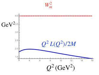
Figure 1: $Q^{2}L(Q^{2})/2M\,{\it vs.}\,W_{m}^{2}$

Prior to evaluating $q(x)$ it is useful and possible to see if the sum rule of Eq. (12) is satisfied. The right hand side of that equation is to be obtained by the high $Q^{2}$ expression for $q(x)$. This quantity is obtained from Eq. (3) by using the field expansion, in the standard expressions of the two-parton Fock-space component wave function. The result using the model of Sect. IV is that

$$q(x)=\int d^{2}b\big{|}\psi_{00}(b,x)\big{|}^{2}=1.$$ (61)

This expression involves an integral over all values of ${\bf b}$ and therefore is equivalent to an integral over all values of ${\bf k}$. This latter integral corresponds to an infinite momentum transfer scale Lepage and Brodsky (1980). Thus QCD evolution of the distributions is not discussed further. The $Q^{2}$ dependence of $q(x,Q^{2})$ of Eq. (26) arises from the $Q^{2}$ dependence of the resonance form factors.

The result $q(x)=1$ requires further comment because it displays the unrealistic nature of the present model. According to quark counting rules, see e.g. Brodsky et al. (1995), the structure function of a two-parton state should fall as $1-x$ for large values of $x$, with QCD-DGLAP evolution providing a faster fall-off. Bloom and Gilman Bloom and Gilman (1970, 1971) use quark counting rules in the form of the Drell-Yan-West Drell and Yan (1970a); West (1970) relations to understand their duality. As shown by Drell and Yan Drell and Yan (1970a), a quark structure function varies at large $x$ as $(1-x)^{2n-1}$ if the corresponding form factor $F(Q^{2})\sim(1/Q^{2})^{n}$ at large values of $Q^{2}$. The present model violates this relation because, as shown above, all of the form factors have the same asymptotic $1/Q^{2}$ behavior, but the structure function is constant. In the present model, the asymptotic nature of the form factor is determined by the Feynman mechanism. The quark counting rules are based on vector meson exchange between the quarks, so that the important region occurs when all of the partons are on top of each other. Feynman Feynman (1972) argued that is not realistic.

The validity of the Feynman vs quark-counting picture is one of the important issues related to color transparency Frankfurt et al. (1994), the interesting quantum invisibility predicted to occur as the result of vanishing of initial or final-state interactions. Color transparency cannot occur if the Feynman mechanism is dominant Frankfurt et al. (1993).

The purpose of the present paper is to investigate the stated model. Although simple it has the correct completeness and support properties that enable study of Bloom-Gilman duality. Therefore we investigate the sum rule Eq. (12) by using $q(x)=1$. This allows the right-hand-side $\equiv R(Q^{2})$ of Eq. (12) to be evaluated immediately:

$$R(Q^{2})\equiv\int_{1}^{1+W_{m}^{2}/Q^{2}}d\omega^{\prime}\nu W_{2}(\omega^{\prime})=2M\int_{1}^{1+W_{m}^{2}/Q^{2}}d\omega^{\prime}x,$$ (62)

with $x=1/(\omega^{\prime}-M^{2}/Q^{2})$. Evaluation yields

$$R(Q^{2})=2M\ln{Q^{2}+W_{m}^{2}-M^{2}\over Q^{2}-M^{2}},$$ (63)

and

$$\lim_{Q^{2}\to\infty}R(Q^{2})=2M{W_{m}^{2}\over Q^{2}}$$ (64)

This result of using the stated model is already in violation of the Bloom-Gilman condition that it be independent of $Q^{2}$. The independence could be obtained by taking $Q^{2}$ to infinity, so that $R\to 0$, and the violation of global duality is assured.

Next examine the left-hand side of Eq. (12) ($\equiv L(Q^{2})$). First that the lower limit on the integral over $\nu$ is determined by the largest value of $x\,(=1)$ for which $\nu W_{2}$ is non-zero. This is given by $Q^{2}/(2M)$. Converting the integral over $\nu$ to one over $x$ gives

$$L(Q^{2})={2M}\int^{1}_{Q^{2}\over(Q^{2}+W_{m}^{2}-M^{2})}{dx\over x}q(x,Q^{2})$$ (65)

in which $q(x,Q^{2})$ is to be obtained from the hadronic expression, Eq. (10) . Simplifying the argument of the delta function leads to:

$$q(x,Q^{2})=\sum_{X}|F_{X}(Q)|^{2}\delta(x-x_{X}),$$ (66)

where $X\equiv(n,L_{z},{\cal L})$ and $x_{X}={Q^{2}\over Q^{2}+2\kappa^{2}(2n+L+{\cal L}({\cal L}+1))}.$

Thus

$$L(Q^{2})=2M\sum_{n,L_{z},{\cal L}}{Q^{2}+2\kappa^{2}(2n+L+{\cal L}({\cal L}+1))\over Q^{2}}F^{2}_{nL_{z}{\cal L}}(Q^{2})\Theta(W_{m}^{2}-2\kappa^{2}(2n+L+{\cal L}({\cal L}+1))$$ (67)

If $R$ were equal to $L$ the sum appearing in Eq. (67) would need to vary as $1/Q^{2}$. This seems unlikely because for finite values of $M_{X}^{2}$, each form factor varies as $1/Q^{2}$, leading to an overall dependence varying approximately as $1/Q^{4}$. The asymptotic limit is not precisely accurate, but nevertheless $L(Q^{2})$ falls much faster than $1/Q^{2}$.

This dependence is shown in Fig. 1. To obtain this figure we take $M^{2}=2\kappa^{2}$, with $M$ the nucleon mass and $W_{m}=2$ GeV, so that $2n+L+2{\cal L}({\cal L}+1)\leq 4$. The result is shown in Fig. 1. Global duality would hold if $Q^{2}R(Q^{2})/2M=Q^{2}L(Q^{2})/2M$ i.e, if the blue and red curves were equal.

X Bloom Gilman Local Duality is not satisfied by the model

Local duality is studied through Eq. (13). If the upper and lower limits are taken to encompass one resonance, $X$, this equation leads to the relation

$${1\over x_{X}}F^{2}_{X}=\ln{W_{+}^{2}+Q^{2}-M^{2}\over W_{-}^{2}+Q^{2}-M^{2}},$$ (68)

with $W_{\pm}=M_{X}\pm\gamma/2$. Here the value of $\gamma$ can be any energy less than the minimum spacing between levels, $2\kappa^{2}$. A first glance indicates that the relation Eq. (68) is not generally satisfied because the right hand side depends on $\gamma$, but the left hand side does not. Moreover, the right-hand side falls as $1/Q^{2}$ for large values of $Q^{2}$, but the left-hand side falls as $1/Q^{4}$.

An explicit calculation is made by choosing the lowest energy resonance with $n=0,\,L=1.\,\,{\cal L}=0$ as an example. The results, shown in Fig. 2 are that indeed the local duality relation is not satisfied.

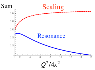
Figure 2: Left- (blue, dashed,Resonance) and right- (red,solid,Scaling) hand sides of Eq. (68) times $Q^{2}/4\kappa^{2}$, with $\gamma=0.125\kappa$.

XI Evaluate $q(x,Q^{2})$

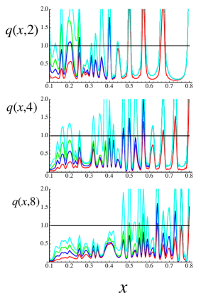
Figure 3: $q(x,z)$ for $z=Q^{2}/4\kappa^{2}\,=\,2,\,4,\,8$. The four curves in each figure are $q_{{\cal L}=0}(x),\,q_{{\cal L}=0}(x)+q_{{\cal L}=1}(x),q_{{\cal L}=0}(x)+q_{{\cal L}=1}(x)+q_{{\cal L}=2}(x),\,q_{{\cal L}=0}(x)+q_{{\cal L}=1}(x)+q_{{\cal L}=2}(x)+q_{{\cal L}=3}(x).$

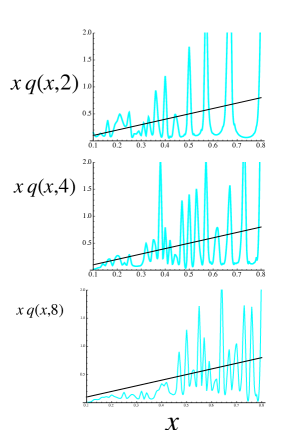
Figure 4: $x(q_{{\cal L}=0}(x,z)+q_{{\cal L}=1}(x)+q_{{\cal L}=2}(x)+q_{{\cal L}=3}(x))$ for $z=Q^{2}/4\kappa^{2}\,=\,2,\,4,\,8$. The lines are drawn to guide the eye.

The quantity to evaluate is $q(x,Q^{2})$ of Eq. (26). The need to include a non-zero width of the excited states in studying duality has been noted in Isgur et al. (2001); Jeschonnek and Van Orden (2004). Moreover, excited states do have non-zero widths. This is addressed next using a Breit-Wigner form.

The starting point is the function $\delta(M^{2}-M_{X}^{2}+Q^{2}(1/x-1)=\delta(M_{X}^{2}-W^{2}),$ where $W^{2}=(p+q)^{2}$. The value of $x$ that yields a vanishing argument is defined to be $x_{X}$ with

$$x_{X}(Q^{2})={Q^{2}\over M_{X}^{2}-M^{2}+Q^{2}},$$ (69)

showing that the contribution of a given resonance moves to larger values of $x$ as the value of $Q^{2}$ increases.

It is useful to relate $\delta(W^{2}-M_{X}^{2})$ to a delta function $\delta(x-x_{X})$, allowing a direct study of the new global duality of Sect. V. This may be done by first using $\delta(M_{X}^{2}-W^{2})={1\over 2W}\delta(M_{X}-W)={1\over 2W}\lim_{\Gamma\to 0}{1\over\pi}{\Gamma/2\over W-M_{X}+i\Gamma/2}$. Then apply a small-width approximation, $W-M_{X}=\sqrt{Q^{2}({1\over x}-1)+M^{2}}-\sqrt{{Q^{2}({1\over x_{X}}-1)+M^{2}}}\approx-(x-x_{X}){Q^{2}\over 2M_{X}x_{X}^{2}}$ so that

$$\delta(M_{X}^{2}-W^{2})\to{\Gamma_{X}\over\pi}{M_{X}x_{X}^{4}\over Q^{4}(x-x_{X})^{2}+\Gamma_{X}^{2}x_{X}^{4}M_{X}^{2})}\equiv\hat{\delta}(W^{2}-M_{X}^{2}),$$ (70)

The final step is to make the appearance of $\delta(x-x_{X})$ explicit:

$$\hat{\delta}(W^{2}-M_{X}^{2})={1\over\pi}{\varepsilon_{X}\over(x-x_{X})^{2}+\varepsilon_{X}^{2}}{x_{X}^{2}\over Q^{2}}=\hat{\delta}(x-x_{X}){x_{X}^{2}\over Q^{2}}$$ (71)

with $\varepsilon_{X}\equiv{\Gamma_{X}M_{X}x_{X}^{2}\over Q^{2}}$. Then

$$q(x,Q^{2})=\sum_{X}\,{x_{X}^{2}\over x^{2}}\big{|}F_{X}(Q^{2})\big{|}f\hat{\delta}(x-x_{X})\equiv\sum_{{\cal L}=0}^{3}q_{\cal L}(x,Q^{2}).$$ (72)

The factor $f$ is insures that $\int_{0}^{1}dx\hat{\delta}(x-x_{X})=1$, and $f$ approaches unity as $\varepsilon_{X}$ approaches 0. The second form shows the sum of states with different values of ${\cal L}$. Each $q_{\cal L}(x,Q^{2})$ includes a sum over values of $n$ and $L_{z}$. A maximum value of ${\cal L}=3$ is used. Although, not complete, this is sufficient to display the main points, and is necessary because an infinite number of values is needed for completeness.

The next step is evaluate Eq. (72). Note that the sum over $X$ involves summing over $n,L_{z}=\pm L$ and ${\cal L}$, including all states The results of evaluating Eq. (72) are shown for $z=Q^{2}/(4\kappa)=2,4,8$ in Fig.3. This corresponds to $Q^{2}=8,16,32\kappa^{2}=4,8,16\,\rm M^{2}$. The width is taken as $\Gamma/\kappa=0.05=0.2M/\sqrt{2}$. This is a constant width of space 66 MeV, with $M$ as the nucleon mass. In the spirit of the model, the width is taken to be small Isgur et al. (2001); Jeschonnek and Van Orden (2004). The maximum number of states in the sum Eq. (72) is increased until convergence is reached. In each figure the lowest curve is obtained using ${\cal L}=0$, then the effects of ${\cal L}=1$ are added leading to the next lowest curve. Then the effects of adding states with ${\cal L}=2$ and ${\cal L}=3$ are included and result in two more curves.

Focusing first on $z=2$ and examining the lowest curve, one sees a spiky structure due to the resonance curves. Decreasing the value of the width leads to similar results, with narrower widths and higher peaks. The same pattern is obtained when adding the effects of states with ${\cal L}>0$, with different values of $M_{X}$, Eq. (41), leading to different peaks that increase the distribution function at low values of $x$, as expected from Eq. (69). The contributions of states with ${\cal L}>0$ don’t contribute at higher values of $x$ due to the delta function appearing in Eq. (72). The solid line in each panel shows the scaling result $q(x)=1$. The resonance curves oscillate about the scaling curve for the larger values of $x$, but not for the lower ones.

The patterns for different values of ${\cal L}$ are also seen as the value of $z$ increases. A detailed difference the effect at high values of $x$ are larger. Another is that the curves fall further below the scaling result, and the general tendency of the magnitude of $q(x,Q^{2})$ to decrease as $Q^{2}$ increases is seen. This is another example of the model’s failure to achieve local duality.

The Bloom & Gilman work found duality in $\nu W_{2}$ which is proportional to $xq(x)$. Plots of that quantity are shown in Fig. 4. The lines show $xq(x)=x$ This figure shows that $xq(x,Q^{2})$ does approximately oscillate about a line. This is true, in part, because including the factor $x$ suppresses the region for which the result of using the sum of resonances, Eq. (72) falls below $q(x)=1$. We denote this approximate oscillation as accidental duality, because the detailed evaluations of both global and local duality expressions Eq. (12) and Eq. (13) show a failure to achieve the necessary equality.

These presented results do not demonstrate that the use of hadronic degrees of freedom leads to the equality of the sum, Eq. (72) with the correct model quark distribution $q(x)=1$. This is expected because it is only possible to include a finite number of excitations $X$ and because of the necessity of including a non-zero width to obtain finite values of $q(x,Q^{2})$. However, but they do show that adding intermediate states of higher and higher masses tends toward that direction. This is because adding states of higher mass tends to fill in gaps left by including only lower mass states.

XII Summary and Discussion

Light front wave functions motivated by holographic constructions are used to study $\rm Bloom-Gilman\,duality$ in this paper. Expressions for the structure functions in terms of quark Eq. (3) and hadronic Eq. (10) degrees of freedom (involving transition form factors) are presented, with an ultimate goal of obtaining a relationship between the two expressions. The specific two-parton model is defined in Sect. IV, with masses, Eq. (21), and light front wave functions, Eq. (22), that had been obtained in original work. Transition form factors are expressed, using the Drell-Yan frame, in terms of these wave functions in Eq. (23).

The valence quark-number sum rule is presented as a new form of global duality (integral over all values of $x$ between 0 and 1) in Sect. V, specifically in Eq. (27) and Eq. (28). Using a complete set of hadronic states is necessary for this new global duality to be achieved, Eq. (28). That the original work does not provide a complete set is shown in Eq. (36). The lack of completeness arises from the choice in the original work to examine the presumably dominant configuration of the modes of lowest energy in which the longitudinal wave function of Eq. (15) is given by $X(x)=\sqrt{x(1-x)}$. This single form is not sufficient to provide a complete set in $x$-space. The lack of completeness is remedied by including a longitudinal potential, $U_{\cal L}(x)$, Eq. (37), where ${\cal L}$ is an integer quantum number, for which the stated $X(x)$ is the lowest energy mode with ${\cal L}=0$. The overall strength, $\lambda$, of $U_{\cal L}$ is arbitrarily chosen here. In principle, this parameter, along with the longitudinal potential, should be chosen by some symmetry principle that is unknown to us. The final result should achieve rotational invariance in the model, in the sense of having states with the proper degeneracy. This achievement is left as a goal of future research. Nevertheless, the present complete set is sufficient to carry out the specific purpose of this manuscript which is to examine $\rm Bloom-Gilman\,duality$.

Given the complete set of wave functions, specific expressions for the transition form factors are obtained in Eq. (44), Eq. (46) and Eq. (60). All of the form factors fall as $1/Q^{2}$, Eq. (52), at asymptotically large values. This behavior originates in the dominance of the Feynman mechanism for this model. That the dominant transition form factors have the same asymptotic dependence is one of the requirements to achieve $\rm Bloom-Gilman\,duality$. However, the Drell-Yan connection between form factors and structure functions is also needed, and this feature is absent in the current model.

The model transition form factors are used to assess the validity of the global, Eq. (11), and local, Eq. (12) duality sum rules. The simplicity of the scaling quark distribution in the given model, $q(x)=1$, readily enables studies of these sum rules, with the result that both are not satisfied within the given model. See Figs. 1,2.

Evaluations of the hadronic expression for $q(x,Q^{2})$, Eq. (72) are presented in the previous section, see Figs. 3, 4. The need to obtain non-infinite values to make plots of finite size mandates that the resonant states have at least a small width, as implemented in Eq. (71). The value of the width is chosen to be a small number $66$ MeV. Detailed results depend upon the precise value, but the qualitative conclusions do not. The Figures show that including the states with ${\cal L}>0$ are needed to approach $\rm Bloom-Gilman\,duality$, but that this duality is not obtainable with the present model.

The failure to achieve $\rm Bloom-Gilman\,duality$ is not a failure of the current model because this property should be generally unexpected. Indeed, the lack of $\rm Bloom-Gilman\,duality$ teaches us an important lesson. One might use either hadronic or quark degrees of freedom according to which leads to the simpler description of the specific problem at hand. Since both sets of states are complete, it is natural to expect that $\rm Bloom-Gilman\,duality$ should result. The present work shows that such a supposition is not correct. Instead, the observed validity of both global and local forms of duality for deep inelastic scattering must be related to a deeper feature of QCD.

Although the present model is very simple, it suggests a prediction that if deep inelastic scattering experiments were to be made on the pion, $\rm Bloom-Gilman\,duality$ would not be observed. This is because of the quark-anti-quark structure of the valence wave function that generally leads to a $1/Q^{2}$ behavior of form factors at high momentum transfer.

Bloom & Gilman understood their duality in terms of the asymptotic fall of resonance transition form factors, quark counting rules and a simple scaling function to represent the high $Q^{2}$ data.. The finer details of this analysis have not withstood the test of time, but measurements have shown that their duality still is viable. The underlying origin of this phenomenon is deeply buried within the confinement aspects of QCD. Its ultimate understanding remains a mystery.

References

- Melnitchouk et al. (2005) W. Melnitchouk, R. Ent, and C. Keppel, “Quark-hadron duality in electron scattering,” Phys. Rept. 406, 127–301 (2005), arXiv:hep-ph/0501217 .
- Bloom and Gilman (1970) Elliott D. Bloom and Frederick J. Gilman, “Scaling, Duality, and the Behavior of Resonances in Inelastic electron-Proton Scattering,” Phys. Rev. Lett. 25, 1140 (1970).
- Bloom and Gilman (1971) Elliott D. Bloom and Frederick J. Gilman, “Scaling and the Behavior of Nucleon Resonances in Inelastic electron-Nucleon Scattering,” Phys. Rev. D 4, 2901 (1971).
- De Rujula et al. (1976) A. De Rujula, Howard Georgi, and H.David Politzer, “An Explanation of Local Duality and Precocious Scaling,” Phys. Lett. B 64, 428–432 (1976).
- De Rujula et al. (1977) Alvaro De Rujula, Howard Georgi, and H.David Politzer, “Demythification of Electroproduction, Local Duality and Precocious Scaling,” Annals Phys. 103, 315 (1977).
- Niculescu et al. (2000a) I. Niculescu et al., “Experimental verification of quark hadron duality,” Phys. Rev. Lett. 85, 1186–1189 (2000a).
- Niculescu et al. (2000b) I. Niculescu et al., “Evidence for valencelike quark hadron duality,” Phys. Rev. Lett. 85, 1182–1185 (2000b).
- Ent et al. (2000) R. Ent, C.E. Keppel, and I. Niculescu, “Nucleon elastic form-factors and local duality,” Phys. Rev. D 62, 073008 (2000).
- Einhorn (1976) Martin B. Einhorn, “Confinement, form factors, and deep-inelastic scattering in two-dimensional quantum chromodynamics,” Phys. Rev. D 14, 3451–3471 (1976).
- Domokos et al. (1971a) G. Domokos, S. Kovesi-Domokos, and E. Schonberg, “Direct-channel resonance model of deep-inelastic electron scattering. i. scattering on unpolarized targets,” Phys. Rev. D 3, 1184–1190 (1971a).
- Domokos et al. (1971b) G. Domokos, S. Kovesi-Domokos, and E. Schonberg, “Deep-inelastic neutrino scattering in a resonance model,” Phys. Rev. D 4, 2115–2125 (1971b).
- Isgur et al. (2001) Nathan Isgur, Sabine. Jeschonnek, W. Melnitchouk, and J.W. Van Orden, “Quark hadron duality in structure functions,” Phys. Rev. D 64, 054005 (2001), arXiv:hep-ph/0104022 .
- Jeschonnek and Van Orden (2004) Sabine Jeschonnek and J.W. Van Orden, “Modeling quark hadron duality for relativistic, confined fermions,” Phys. Rev. D 69, 054006 (2004), arXiv:hep-ph/0310298 .
- Close and Zhao (2002) Frank E. Close and Qiang Zhao, “A Pedagogic model for deeply virtual Compton scattering with quark hadron duality,” Phys. Rev. D 66, 054001 (2002), arXiv:hep-ph/0202181 .
- Harrington (2002) David R. Harrington, “Asymptotic freedom for nonrelativistic confinement,” Phys. Rev. C 66, 065205 (2002).
- Close and Isgur (2001) Frank E. Close and Nathan Isgur, “The Origins of quark hadron duality: How does the square of the sum become the sum of the squares?” Phys. Lett. B 509, 81–86 (2001), arXiv:hep-ph/0102067 .
- Paris and Pandharipande (2001) M.W. Paris and Vijay R. Pandharipande, “Scaling of space and time - like response of confined relativistic particles,” Phys. Lett. B 514, 361–365 (2001), arXiv:nucl-th/0105076 .
- Paris and Pandharipande (2002) Mark W. Paris and Vijay R. Pandharipande, “Final state interaction contribution to the response of confined relativistic particles,” Phys. Rev. C 65, 035203 (2002).
- Brodsky et al. (2015) Stanley J. Brodsky, Guy F. de Teramond, Hans Gunter Dosch, and Joshua Erlich, “Light-Front Holographic QCD and Emerging Confinement,” Phys. Rept. 584, 1–105 (2015), arXiv:1407.8131 [hep-ph] .
- Brodsky et al. (1998) Stanley J. Brodsky, Hans-Christian Pauli, and Stephen S. Pinsky, “Quantum chromodynamics and other field theories on the light cone,” Phys. Rept. 301, 299–486 (1998), arXiv:hep-ph/9705477 .
- Dirac (1949) Paul A.M. Dirac, “Forms of Relativistic Dynamics,” Rev. Mod. Phys. 21, 392–399 (1949).
- de Teramond and Brodsky (2009) Guy F. de Teramond and Stanley J. Brodsky, “Light-Front Holography: A First Approximation to QCD,” Phys. Rev. Lett. 102, 081601 (2009), arXiv:0809.4899 [hep-ph] .
- Brodsky and de Teramond (2006) Stanley J. Brodsky and Guy F. de Teramond, “Hadronic spectra and light-front wavefunctions in holographic QCD,” Phys. Rev. Lett. 96, 201601 (2006), arXiv:hep-ph/0602252 .
- Brodsky and de Teramond (2008a) Stanley J. Brodsky and Guy F. de Teramond, “Light-Front Dynamics and AdS/QCD Correspondence: The Pion Form Factor in the Space- and Time-Like Regions,” Phys. Rev. D 77, 056007 (2008a), arXiv:0707.3859 [hep-ph] .
- Polchinski and Strassler (2003) Joseph Polchinski and Matthew J. Strassler, “Deep inelastic scattering and gauge / string duality,” JHEP 05, 012 (2003), arXiv:hep-th/0209211 .
- Drell and Yan (1970a) S.D. Drell and Tung-Mow Yan, “Connection of Elastic Electromagnetic Nucleon Form-Factors at Large Q**2 and Deep Inelastic Structure Functions Near Threshold,” Phys. Rev. Lett. 24, 181–185 (1970a).
- West (1970) Geoffrey B. West, “Phenomenological model for the electromagnetic structure of the proton,” Phys. Rev. Lett. 24, 1206–1209 (1970).
- Brodsky and de Teramond (2008b) Stanley J. Brodsky and Guy F. de Teramond, “Light-Front Dynamics and AdS/QCD Correspondence: Gravitational Form Factors of Composite Hadrons,” Phys. Rev. D 78, 025032 (2008b), arXiv:0804.0452 [hep-ph] .
- Abidin and Carlson (2008) Zainul Abidin and Carl E. Carlson, “Gravitational form factors of vector mesons in an AdS/QCD model,” Phys. Rev. D 77, 095007 (2008), arXiv:0801.3839 [hep-ph] .
- Drell and Yan (1970b) Sidney D. Drell and Tung-Mow Yan, “Connection of elastic electromagnetic nucleon form factors at large and deep inelastic structure functions near threshold,” Phys. Rev. Lett. 24, 181–186 (1970b).
- Karch et al. (2006) Andreas Karch, Emanuel Katz, Dam T. Son, and Mikhail A. Stephanov, “Linear confinement and AdS/QCD,” Phys. Rev. D 74, 015005 (2006), arXiv:hep-ph/0602229 .
- de Téramond and Brodsky (2009) Guy F. de Téramond and Stanley J. Brodsky, “Light-front holography: A first approximation to qcd,” Phys. Rev. Lett. 102, 081601 (2009).
- de Téramond et al. (2015) Guy F. de Téramond, Hans Günter Dosch, and Stanley J. Brodsky, “Baryon spectrum from superconformal quantum mechanics and its light-front holographic embedding,” Phys. Rev. D 91, 045040 (2015).
- Dosch et al. (2015) Hans Günter Dosch, Guy F. de Téramond, and Stanley J. Brodsky, “Superconformal baryon-meson symmetry and light-front holographic qcd,” Phys. Rev. D 91, 085016 (2015).
- Lepage and Brodsky (1980) G.Peter Lepage and Stanley J. Brodsky, “Exclusive Processes in Perturbative Quantum Chromodynamics,” Phys. Rev. D 22, 2157 (1980).
- Li et al. (2016) Yang Li, Pieter Maris, Xingbo Zhao, and James P. Vary, “Heavy Quarkonium in a Holographic Basis,” Phys. Lett. B 758, 118–124 (2016), arXiv:1509.07212 [hep-ph] .
- Miller and Brodsky (2020) Gerald A. Miller and Stanley J. Brodsky, “Frame-independent spatial coordinate : Implications for light-front wave functions, deep inelastic scattering, light-front holography, and lattice QCD calculations,” Phys. Rev. C 102, 022201 (2020), arXiv:1912.08911 [hep-ph] .
- Feynman (1972) R.P. Feynman, Photon-hadron interactions (W.A. Benjamin, Inc., Reading, 1972).
- Brodsky et al. (1995) Stanley J. Brodsky, Matthias Burkardt, and Ivan Schmidt, “Perturbative QCD constraints on the shape of polarized quark and gluon distributions,” Nucl. Phys. B 441, 197–214 (1995), arXiv:hep-ph/9401328 .
- Frankfurt et al. (1994) L.L. Frankfurt, G.A. Miller, and M. Strikman, “The Geometrical color optics of coherent high-energy processes,” Ann. Rev. Nucl. Part. Sci. 44, 501–560 (1994), arXiv:hep-ph/9407274 .
- Frankfurt et al. (1993) L. Frankfurt, G.A. Miller, and M. Strikman, “Precocious dominance of point - like configurations in hadronic form-factors,” Nucl. Phys. A 555, 752–764 (1993).