Gauge Principle and Gauge Invariance in Two-Level Systems

Abstract

The quantum Rabi model is a widespread description of the coupling between a two-level system and a quantized single mode of an electromagnetic resonator. Issues about this model’s gauge invariance have been raised. These issues become evident when the light-matter interaction reaches the so-called ultrastrong coupling regime. Recently, a modified quantum Rabi model able to provide gauge-invariant physical results (e.g., energy levels, expectation values of observables, quantum probabilities) in any interaction regime was introduced [Nature Physics 15, 803 (2019)]. Here we provide an alternative derivation of this result, based on the implementation in two-state systems of the gauge principle, which is the principle from which all the fundamental interactions in quantum field theory are derived. The adopted procedure can be regarded as the two-site version of the general method used to implement the gauge principle in lattice gauge theories. Applying this method, we also obtain the gauge-invariant quantum Rabi model for asymmetric two-state systems, and the multi-mode gauge-invariant quantum Rabi model beyond the dipole approximation.

I Introduction

Recently, it has been argued that truncations of the atomic Hilbert space, to obtain a two-level description of the matter system, violate the gauge principle [1, 2, 3]. Such violations become particularly relevant in the ultrastrong and deep-strong coupling (USC and DSC) regimes. These extreme regimes have been realized between individual or collections of effective two-level systems (TLSs) and the electromagnetic field in a variety of settings [4, 5]. In the USC (DSC) regime of quantum light-matter interaction the coupling strength becomes comparable (larger) than the transition frequencies of the system.

Reference et al. [1] demonstrated that, while in the electric dipole gauge, the two-level approximation can be performed as long as the Rabi frequency remains much smaller than the energies of all higher-lying levels. The two-level approximation can drastically fail in the Coulomb gauge, even for systems with an extremely anharmonic spectrum.

The impact of the truncation of the Hilbert space of the matter system to only two states was also studied  [2], by introducing a one-parameter ($\alpha$) set of gauge transformations. The authors found that each value of the parameter produces a distinct quantum Rabi model (QRM), thus providing distinct physical predictions. Investigating a matter system with a lower anharmonicity (with respect to that considered in Ref. [1]), they use the gauge parameter $\alpha$ as a fit parameter to determine the optimal QRM for a specific set of system parameters, by comparing the obtained $\alpha$-dependent lowest energy states and levels with the corresponding predictions of the non-truncated gauge invariant model. The surprising result [2] is that, according to this procedure, in several circumstances the optimal gauge is the so-called Jaynes-Cummings (JC) gauge, a gauge where the counter-rotating terms are automatically absent.

Recently, the source of gauge violation has been identified  [6], and a general method for the derivation of light-matter Hamiltonians in truncated Hilbert spaces able to produce gauge-invariant physical results has been developed [6] (see also related work [7, 8, 9]). This gauge invariance was achieved by compensating the non-localities introduced in the construction of the effective Hamiltonians. Consequently, the resulting quantum Rabi Hamiltonian in the Coulomb gauge differs significantly from the standard one, but provides exactly the same energy levels obtained by using the dipole gauge, as it should, because physical observable quantities must be gauge invariant. A recent overview of these gauge issues in TLSs can be found in Ref. [10].

Very recently, the validity of the gauge invariant QRM developed in Ref. [6] has been put into question [3]. Specifically, it is claimed that the truncation of the Hilbert space necessarily ruins gauge-invariance.

In this paper, however, we confirm that the gauge principle applies also to TLSs, as required by any consistent description of light-matter interaction. Specifically, we formulate in a fully consistent and physically meaningful way the fundamental gauge principle in two-state systems. The derivation described here can be regarded as the two-site version of the general method for lattice gauge theories [11]. These represent the most advanced and commonly used tool for describing gauge theories in the presence of a truncated infinite-dimensional Hilbert space. When a gauge theory is regularized on the lattice, it is vital to maintain its invariance under gauge transformations [11]. An analogous approach has been developed as early as 1933 [12] for the description of tightly-bound electrons in a crystal in the presence of a slowly-varying magnetic vector potential (see, e.g., also Refs. [13, 14, 15]). Applying this method, we also obtain the multi-mode gauge-invariant QRM beyond the dipole approximation.

II The gauge principle

In this section, we recall some fundamental concepts, which we will apply in the next sections.

In quantum field theory, the coupling of particles with fields is constructed in such a way that the theory is invariant under a gauge transformation [16]. Here, we limit the theoretical model to consider $U(1)$ invariance. For symmetry groups that are non-commutative, this approach can be generalized to non-abelian gauge theories [16, 11].

Let us consider the transformation of the particle field $\psi\to\exp(iq\theta)\psi$. This transformation represents a symmetry of the free action of the particle (e.g., the Dirac action) if $\theta$ is a constant, but we want to consider a generic function $\theta(x)$ (local phase transformation). However, the free Dirac action is not invariant under local phase transformations, because the factor $\exp[iq\theta(x)]$ does not commute with $\partial_{\mu}$. At the same time, it is known that the action of the free electromagnetic field is invariant under the following gauge transformation:

$$A_{\mu}\to A_{\mu}-\partial_{\mu}{\theta}\,.$$ (1)

It is then possible to replace, in the action, the derivative $\partial_{\mu}$ with a covariant derivative of $\psi$ as

$$D_{\mu}\psi=\left(\partial_{\mu}+iqA_{\mu}\right)\psi\,,$$ (2)

so that

$$D_{\mu}\psi\to e^{iq\theta}D_{\mu}\psi\,,$$ (3)

even when $\theta$ depends on $x$. It is now easy to construct a Lagrangian with a local $U(1)$ invariance. It suffices to replace all derivatives $\partial_{\mu}$ with covariant derivatives $D_{\mu}$.

The same procedure, leading to the well-known minimal coupling replacement, can be applied to describe the interaction of a non-relativistic particle with the electromagnetic field. Considering a particle of mass $m$ with a geometrical coordinate $x$ and a potential $V(x)$, the Hamiltonian of such a particle interacting with the electromagnetic field can be written as

$$\hat{H}_{0}^{\rm gi}=\frac{1}{2m}\left[\hat{p}-qA(x)\right]^{2}+V(x)\,,$$ (4)

where $\hat{p}=-id/dx$ is the momentum of the particle (here $\hbar=1$). It turns out that the expectation values $\langle\psi|\hat{H}_{0}^{\rm gi}|\psi\rangle$ are invariant under local phase transformations,

$$\psi(x)\to e^{iq\theta(x)}\psi(x)\,,$$ (5)

thanks to the presence of the gauge field $A(x)$.

Note that the function of a continuous degree of freedom $\psi(x)$ lives in the infinite-dimensional space of all square-integrable functions, and the local phase transformation transforms a state vector in this space into a different vector in the same space. Finally, we observe that the total Hamiltonian, in addition to $\hat{H}_{0}^{\rm gi}$, includes the free Hamiltonian for the gauge field.

III Double-well systems in the two-state limit

The problem of a quantum-mechanical system whose state is effectively restricted to a two-dimensional Hilbert space is ubiquitous in physics and chemistry [17]. In the simplest examples, the system simply possesses a degree of freedom that can take only two values. For example, the spin projection in the case of a spin-$1/2$ particle or the polarization in the case of a photon. Besides these intrinsically two-state systems, a more common situation is that the system has a continuous degree of freedom $x$, for example, a geometrical coordinate, and a potential energy function $V(x)$ depending on it, with two separate minima [17] (see Fig. 1).

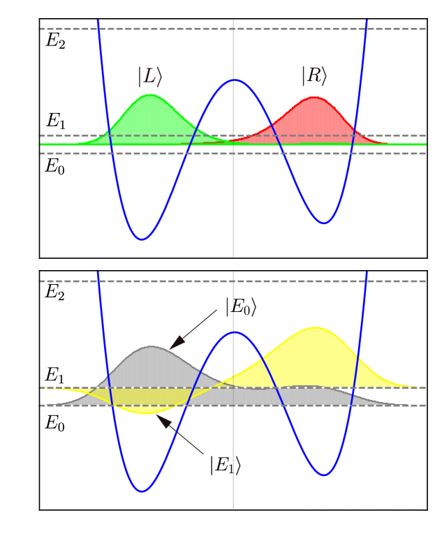
Figure 1: A double-well system in the two-state limit. The symbols $E_{0}$ and $E_{1}$ are the two lowest-energy levels, well separated in energy by the next higher energy level $E_{2}$. Panel (a) also shows the square modulus of the two wavefunctions localized in the well, obtained as linear combinations of the two lowest energy wavefunctions displayed in panel (b).

Let us assume that the barrier height $V$ is large enough that the system dynamics can be adequately described by a two-dimensional Hilbert space spanned by the two ground states in the two wells $|L\rangle$ and $|R\rangle$.

The motion in the two-dimensional Hilbert space can be adequately described by the simple Hamiltonian:

$$\hat{\cal H}_{0}=\sum_{j=L,R}E_{j}|j\rangle\langle j|-t\left(|R\rangle\langle L|+{\rm h.c.}\right)\,,$$ (6)

where the tunneling coefficient is given by $t=\langle L|\hat{H}_{0}|R\rangle$, and

$$\hat{H}_{0}=\frac{\hat{p}^{2}}{2m}+V(x)$$ (7)

is the usual system Hamiltonian.

If the potential is an even function of the geometrical coordinate, namely $V(x)=V(-x)$ (see Fig. 2), then $E_{L}=E_{R}$, and we can fix $E_{L}=E_{R}=0$. Introducing the Pauli operator $\hat{\rho}_{x}=|L\rangle\langle R|+{\rm h.c.}$, we obtain

$$\hat{\cal H}_{0}=-t\hat{\rho}_{x}\,,$$ (8)

whose eigenstates, delocalized in the two wells, are the well-known symmetric- and antisymmetric combinations (see Fig. 2b),

$$|S\rangle = \frac{1}{\sqrt{2}}\left(|R\rangle+|L\rangle\right)\,,$$

$$|A\rangle = \frac{1}{\sqrt{2}}\left(|R\rangle-|L\rangle\right)\,,$$ (9)

with eigenvalues $E_{A,S}=\pm t$, so that $\Delta=E_{A}-E_{S}=2t$, where we assume $t>0$. The Hamiltonian in Eq. (6) can be written in diagonal form as

$$\hat{\cal H}_{0}=(\Delta/2)\hat{\sigma}_{z}\,,$$ (10)

where $\hat{\sigma}_{z}=-\hat{\rho}_{x}=|A\rangle\langle A|-|S\rangle\langle S|$. Note, to distinguish between the different basis states for the operator representations, we use $\hat{\sigma}_{i}$ for the $|A\rangle{-}|S\rangle$ basis, and $\hat{\rho}_{i}$ for the $|L\rangle{-}|R\rangle$ basis. Thus, for example, the diagonal $\hat{\sigma}_{z}$ operator becomes nondiagonal in the $|L\rangle{-}|R\rangle$ basis.

It is worth noting that this elementary analysis is not restricted to the case of a double-well potential. Analogous considerations can be carried out for systems with different potential shapes, displaying two (e.g., lowest energy) levels well separated in energy from the next higher level. The wavefunctions $\psi_{L}(x)=\langle x|L\rangle$ and $\psi_{R}(x)=\langle x|L\rangle$ can be obtained from the symmetric and antisymmetric combinations of $\psi_{S}(x)$ and $\psi_{A}(x)$ (see Fig. 1), which can be obtained exactly as the two lowest energy eigenfunctions of the Schrödinger problem described by the Hamiltonian in Eq. (7). The gap $\Delta=2t$ is obtained from the difference between the corresponding eigenvalues. This two-state tunneling model is a well known formalism to describe many realistic systems, including the ammonia molecule, coupled quantum dots, and superconducting flux-qubits.

The case of a potential of the effective particle which does not display inversion symmetry can also be easily addressed. For example, consider an asymmetric double well potential, as shown in Fig. 1. In this case, Eq. (6) can be expressed as

$$\hat{\cal H}_{0}=\frac{\epsilon}{2}\hat{\rho}_{z}-\frac{\Delta}{2}\hat{\rho}_{x}\,.$$ (11)

The quantity $\epsilon$ is the detuning parameter, that is, the difference in the ground-state energies of the states localized in the two wells in the absence of tunneling. The Hamiltonian in Eq. (11) can be trivially diagonalized with eigenvalues $\pm\omega_{q}/2$, where $\omega_{q}=\sqrt{\Delta^{2}+\epsilon^{2}}$.

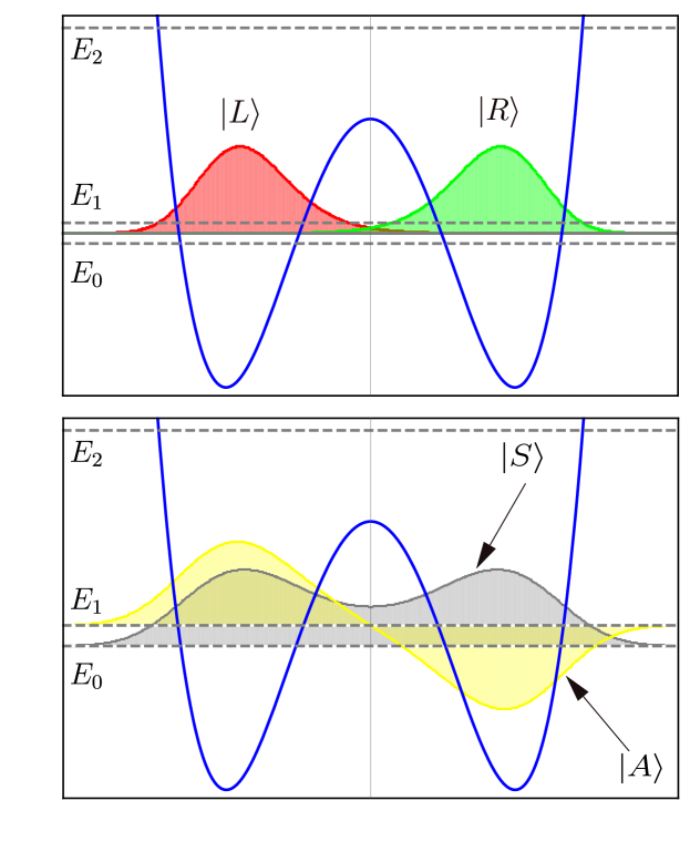
Figure 2: A symmetric double-well system in the two-state limit. The symbols $E_{0}$ and $E_{1}$ are the two lowest-energy levels, well separated in energy by the next higher energy level $E_{2}$. Panel (a) also shows the square modulus of the two wavefunctions localized in the well, obtained as symmetric and antysimmetric combinations of the two lowest energy wavefunctions displayed in panel (b).

IV The gauge principle in two-level systems

The question arises if it is possible to save the gauge principle when, under the conditions described above, such a particle is adequately described by states confined in a two-dimensional complex space. If we apply an arbitrary local phase transformation to, e.g., the wavefunction $\psi_{A}(x)=\langle x|A\rangle$: $\psi_{A}(x)\to\psi^{\prime}_{A}(x)=e^{iq\theta(x)}\psi_{A}(x)$, it happens that, in general, $\psi^{\prime}_{A}(x)\neq c_{S}\psi_{S}(x)+c_{A}\psi_{A}(x)$, where $c_{A}$ and $c_{S}$ are complex coefficients. Thus the general local phase transformation does not guarantee that the system can still be described as a two state system. According to this analysis, those works claiming gauge non-invariance due to material truncation in ultrastrong-coupling QED [18] (we would say at any coupling strength, except negligible), at first sight, might appear to be correct. The direct consequence of this conclusion would be that two-level models, widespread in physics and chemistry, are too simple to implement their interaction with a gauge field, according to the general principle from which the fundamental interactions in physics are obtained. Since adding to the particle system description a few additional levels does not change this point, the conclusion would be even more dramatic. Moreover, according to Ref.s [2, 3], this leads to several non-equivalent models of light-matter interactions providing different physical results. One might then naively claim the “death of the gauge principle” and of gauge invariance in truncated Hilbert spaces, namely in almost all cases where theoreticians try to provide quantitative predictions to be compared with actual experiments.

Our view is drastically different: we find that the breakdown of gauge invariance is the direct consequence of the inconsistent approach of reducing the information (Hilbert space truncation) on the effective particle, without accordingly reducing the information, by the same amount, on the phase $\theta(x)$ determining the transformation in Eq. (5). In physics, the approximations must be done with care, and they must be consistent.

We start by observing that the two-state system defined in Eq. (6) still has a geometric coordinate, which however can assume only two values: $x_{j}$ (with $j=L,R$), that we can approximately identify with the position of the two minima of the double-well potential. More precisely, and more generally, they are:

$$x_{R} = \langle R|x|R\rangle,$$

$$x_{L} = \langle L|x|L\rangle\,.$$ (12)

Here, parity symmetry implies $x_{L}=-x_{R}$. In the following we will use the shorthand $\langle R|x|R\rangle=a/2$. Hence, the operator describing the geometric coordinate can be written as [17] ${\cal X}=(a/2)\hat{\rho}_{z}$, where $\hat{\rho}_{z}\equiv|R\rangle\langle R|-|L\rangle\langle L|$.

We observe that the terms proportional to $t$ in the Hamiltonian in Eq. (6) or Eq. (8), implies that these can be regarded as nonlocal Hamiltonians, i.e., with an effective potential depending on two distinct coordinates. Nonlocality here comes from the hopping term $t=\langle R|\hat{H}_{0}|L\rangle$, which is determined by the interplay of the kinetic energy term and of the potential energy in $\hat{H}_{0}$.

It is clear that the consistent and meaningful local gauge transformation corresponds to the following transformation:

$$|\psi\rangle=c_{L}|L\rangle+c_{R}|R\rangle\to|\psi^{\prime}\rangle=e^{iq\theta_{L}}c_{L}|L\rangle+e^{iq\theta_{R}}c_{R}|R\rangle\,,$$ (13)

where $|\psi\rangle$ is a generic state in the two-dimensional Hilbert space, and $\theta_{j}$ are arbitrary real valued parameters.

It is easy to show that the expectation values of $\hat{\cal H}_{0}$ are not invariant under the local transformation in Eq. (13). They are only invariant under a uniform phase change: $|\psi\rangle\to\exp(iq\theta)|\psi\rangle$. However, one can introduce in the Hamiltonian field-dependent factors, that compensate the difference in the phase transformation from one point to the other. Specifically, following the general procedure of lattice gauge theory, we can consider the parallel transporter (a unitary finite-dimensional matrix), introduced by Kenneth Wilson [19, 20, 11],

$$U_{x_{k}+a,x_{k}}=\exp{\left[iq\int_{x_{k}}^{x_{k}+a}dx\,A(x)\right]}\,,$$ (14)

where $A(x)$ is the gauge field. After the gauge transformation of the field,

$$A^{\prime}(x)=A(x)+d\theta/dx\,,$$ (15)

the transporter transforms as

$$U^{\prime}_{x_{k}+a,x_{k}}=e^{iq\,\theta(x_{k}+a)}U_{x_{k}+a,x_{k}}e^{-iq\,\theta(x_{k})}\,$$ (16)

which is now discrete. This property can also be used to implement gauge invariant Hamiltonians in two-state systems.

IV.1 Symmetric two-state systems

Properly introducing the parallel transporter in Eq. (14) into Eq. (8), we obtain a gauge-invariant two-level model:

$$\hat{\cal H}^{\rm gi}_{0}=-t\,|R\rangle\langle L|\,U_{x_{R},x_{L}}+{\rm h.c.}\,.$$ (17)

Gauge invariance can be directly verified:

$$\langle \psi^{\prime}|\left(|R\rangle\langle L|\,U^{\prime}_{x_{R},x_{L}}+{\rm h.c.}\right)|\phi^{\prime}\rangle=$$

$$\langle \psi|\left(|R\rangle\langle L|\,U_{x_{R},x_{L}}+{\rm h.c.}\right)|\phi\rangle\,,$$

where $|\psi\rangle$ and $|\phi\rangle$ are two generic states in the vector space spanned by $|L\rangle$ and $|R\rangle$. By neglecting the spatial variations of the field potential $A(x)$ on the distance

$$a=x_{R}-x_{L}\,,$$

(dipole approximation). The Hamiltonian in Eq. (17) can be written as

$$\hat{\cal H}^{\rm gi}_{0}=-t\,|R\rangle\langle L|\,e^{iqaA}+{\rm h.c.}\,.$$ (18)

Using Eq. (III) and the Euler formula, it can be easily verified that the Hamiltonian in Eq. (18) can be expressed using the diagonal basis of $\hat{\cal H}_{0}$, as

$$\hat{\cal H}^{\rm gi}_{0}=\frac{\Delta}{2}\left[\hat{\sigma}_{z}\cos{(qaA)}+\hat{\sigma}_{y}\sin{(qaA)}\right]\,,$$ (19)

where $\hat{\sigma}_{y}=-i\left(|A\rangle\langle S|-|S\rangle\langle A|\right)$. Using Eq. (III) and Eq. (IV), then

$$qa/2=q\langle A|x|S\rangle\,.$$ (20)

This precisely coincides with the transition matrix element of the dipole moment as in Ref. [6].

Considering a quantized field $\hat{A}$, the total light-matter Hamiltonian also contains the free-field contribution, $\hat{H}_{\rm ph}$, so that:

$$\hat{\cal H}=\frac{\Delta}{2}\left[\hat{\sigma}_{z}\cos{(qa\hat{A})}+\hat{\sigma}_{y}\sin{(qa\hat{A})}\right]+\hat{H}_{\rm ph}\,.$$ (21)

For the simplest case of a single-mode electromagnetic resonator, the potential can be expanded in terms of the mode photon destruction and creation operators. Around $x=0$, $\hat{A}=A_{0}(\hat{a}+\hat{a}^{\dagger})$, where $A_{0}$ (assumed real) is the zero-point-fluctuation amplitude of the field in the spatial region spanned by the effective particle. We also have: $\hat{H}_{\rm ph}=\omega_{\rm ph}\hat{a}^{\dagger}\hat{a}$, where $\omega_{\rm ph}$ is the resonance frequency of the cavity mode. It can be useful to define the normalized coupling strength parameter [6]

$$\eta=q(a/2)A_{0}\,,$$ (22)

so that Eq. (21) can be written as

$$\hat{\cal H} = \frac{\Delta}{2}\left\{\hat{\sigma}_{z}\cos{[2\eta(\hat{a}+\hat{a}^{\dagger})]}+\hat{\sigma}_{y}\sin{[2\eta(\hat{a}+\hat{a}^{\dagger})]}\right\}$$ (23)

$$+ \omega_{\rm ph}\hat{a}^{\dagger}\hat{a}\,.$$

Using the relations $\hat{\rho}_{z}\equiv|R\rangle\langle R|-|L\rangle\langle L|=|A\rangle\langle S|+|S\rangle\langle A|\equiv\hat{\sigma}_{x}$, the Hamiltonian in Eq. (17) can also be expressed as

$$\hat{\cal H}=\hat{\cal U}\hat{\cal H}_{0}\hat{\cal U}^{\dagger}\,,$$ (24)

where

$$\hat{\cal U}=\exp{(iqa\hat{A}\hat{\sigma}_{x}/2)}\,.$$ (25)

Equations (24) and (25) coincide with Eqs. (8) and (9) of Ref. [6], which represents our main results.

It is also interesting to rewrite the coordinate-dependent phase transformation in Eq. (13) as the application of a unitary operator on the system states. Defining $\phi=(\theta_{R}+\theta_{L})/2$ and $\theta=(\theta_{R}-\theta_{L})/2$, Eq. (13) can be written as

$$|\psi\rangle\to|\psi^{\prime}\rangle=e^{iq\phi}e^{iq\theta\hat{\sigma}_{x}}|\psi\rangle\,.$$ (26)

This shows that the coordinate-dependent phase change of a generic state of a TLS is equivalent to a global phase change, which produces no effect, plus a rotation in the Bloch sphere, which can be compensated by introducing a gauge field as in Eq. (24). Notice also that Eq. (26) coincides with the result presented in the first section of the Supplementary Information of Ref. [6], obtained with a different, but equivalent approach.

In summary, the method presented here can be regarded as the two-site version (with the additional dipole approximation) of the general method for lattice gauge theories [11], which represents the most advanced and sophisticated tool for describing gauge theories in the presence of truncation of infinite-dimensional Hilbert spaces. These results eliminate any concern about the validity of the results presented in Ref. [6], raised by Ref. [3].

We conclude this subsection by noting that Eq. (17) can be also used, without applying the dipole approximation, to obtain the (multi-mode) gauge-invariant quantum Rabi model beyond the dipole approximation. Specifically, without applying the dipole approximation to Eq. (17), after the same steps to obtain Eq. (23), we obtain

$$\hat{\cal H} = \frac{\Delta}{2}\left[\hat{\sigma}_{z}\cos\!{\left(q\!\int^{x_{R}}_{x_{L}}\!dx\,\hat{A}(x)\right)}\right.$$ (27)

$$+ \left.\hat{\sigma}_{y}\sin\!{\left(q\!\int^{x_{R}}_{x_{L}}\!dx\,\hat{A}(x)\right)}\right]+\hat{H}_{\rm ph}\,.$$

One interesting consequence of this result is that it introduces a natural cut-off for the interaction of high energy modes of the electromagnetic field with a TLS. In particular, owing to cancellation effects in the integrals in Eq. (27), the resulting coupling strength between the TLS and the mode goes rapidly to zero when the mode wavelength becomes shorter than $a/2=\langle A|x|S\rangle$. This finding can stimulate further investigations beyond the dipole approximation, without having to introduce a cut-off frequency by hand.

It is worth noticing that this derivation of the gauge-invariant QRM does not require the introduction of an externally controlled two-site lattice spacing, in contrast to general lattice gauge theories. In the present case, the effective spacing $a$ between the two sites is only determined by the transition matrix element of the position operator between the two lowest energy states of the effective particle, $a=2\langle A|x|S\rangle$, which in turn determines the dipole moment of the transition, $qa/2$.

IV.2 Asymmetric two-state systems

The results in this section can be directly generalized to also address the case of a potential of the effective particle which does not display inversion symmetry. It has been shown that the interaction (in the USC and DSC limit) of these TLSs (without inversion symmetry), with photons in resonators, can lead to a number of interesting phenomena [21, 22, 23, 24, 25, 26, 27]. In this case, Eq. (11) provides the bare TLS Hamiltonian. Note that the first term in Eq. (11) is not affected by the two-state local phase transformation in Eq. (13), hence the gauge invariant version of Eq. (11) can be written as

$$\hat{\cal H}^{\rm gi}_{0}=\frac{\epsilon}{2}\hat{\rho}_{z}-\frac{\Delta}{2}\,\left(|R\rangle\langle L|\,U_{x_{R},x_{L}}+{\rm h.c.}\right)\,,$$ (28)

which, in the dipole approximation, reads:

$$\hat{\cal H}^{\rm gi}_{0}=\frac{\epsilon}{2}\hat{\rho}_{z}-\frac{\Delta}{2}\,\left(|R\rangle\langle L|\,e^{iqaA}+{\rm h.c.}\right)\,.$$ (29)

This can be expressed as

$$\hat{\cal H}^{\rm gi}_{0}=\frac{\epsilon}{2}\hat{\rho}_{z}-\frac{\Delta}{2}\left[\hat{\rho}_{x}\cos{(qaA)}-\hat{\rho}_{y}\sin{(qaA)}\right]\,,$$ (30)

which can also be written in the more compact form

$$\hat{\cal H}^{\rm gi}_{0}=\hat{\cal U}\hat{\cal H}_{0}\hat{\cal U}^{\dagger}\,,$$ (31)

where

$$\hat{\cal U}=\exp{\left[iqaA\hat{\rho}_{z}/2\right]}\,.$$ (32)

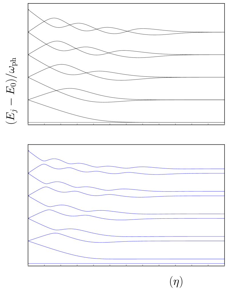
Figure 3: Normalized Energy spectra of the QRMs for the symmetric (a) and asymmetric (b) TLS. Energy differences $(E_{j}-E_{0})/\omega_{\rm ph}$ ($E_{j}$ are energy eigenvalues) as a function of the normalized coupling strength $\eta$, calculated at zero detuning: $\omega_{q}=\omega_{\rm ph}$. Panel (a) displays the spectrum for the standard QRM (symmetric TLS), while the spectrum for the QRM for the asymmetric TLS is shown in (b).

Equations (31) and (32) represent the minimal coupling replacement for TLSs, derived directly from the fundamental gauge principle.

We observe that the operator $\hat{\cal X}=a\hat{\rho}_{z}/2$ represents the geometrical-coordinate operator for the two-state system, with eigenvalues $\pm a/2$. The Hamiltonian in Eq. (30) can be directly generalized beyond the dipole approximation with the following replacement:

$$aA\to\int_{-a/2}^{a/2}\!dx\,A(x)\,.$$ (33)

Considering a single-mode electromagnetic resonator, the total Hamiltonian becomes

$$\hat{\cal H} = \omega_{\rm ph}\hat{a}^{\dagger}\hat{a}+\frac{\epsilon}{2}\hat{\rho}_{z}$$

$$- \frac{\Delta}{2}\left\{\hat{\rho}_{x}\cos{\left[2\eta(\hat{a}+\hat{a}^{\dagger})\right]}-\hat{\rho}_{y}\sin{\left[2\eta(\hat{a}+\hat{a}^{\dagger})\right]}\right\}\,.$$

Since the operator $\hat{\cal X}$ is the position operator in the two-state space, the unitary operator $\hat{\cal U}^{\dagger}=\hat{\cal T}$ also corresponds to the operator which implements the PZW unitary transformation [28], leading to the dipole-gauge representation,

$$\hat{\cal H}_{d} = \hat{\cal U}^{\dagger}\hat{\cal H}\hat{\cal U}=\omega_{\rm ph}\hat{a}^{\dagger}\hat{a}+\frac{\epsilon}{2}\hat{\rho}_{z}-\frac{\Delta}{2}\hat{\rho}_{x}$$ (35)

$$- i\eta\omega_{\rm ph}(\hat{a}-\hat{a}^{\dagger})\hat{\rho}_{z}+\eta^{2}\hat{\cal I}\,,$$

where we used: $\hat{\rho}_{z}^{2}=\hat{\cal I}$, with ${\cal I}$ the identity operator for the two-state system. Note that $\hat{\cal H}_{d}$ coincides with the Hamiltonian describing a flux qubit interacting with an $LC$ oscillator [25].

Since the Hamiltonians in Eq. (IV.2) and Eq. (35) are related by a gauge (unitary) transformation, their eigenvalues $E_{j}$ coincide. Figure 3 displays their energy spectra, defined as $(E_{j}-E_{0})/\omega_{\rm ph}$ as a function of the normalized coupling strength, where $E_{0}$ is the ground state energy. The spectra have been obtained at zero detuning: $\omega_{q}=\omega_{\rm ph}$. In particular, Fig. 3(a) displays the energy spectrum in the absence of symmetry breaking ($\epsilon=0$), namely that of the standard QRM [6]. Panel 3(b) is obtained using $\epsilon=0.2\omega_{\rm ph}$. Such a symmetry breaking gives rise to a number of interesting features. In particular, we observe that the level crossings present in panel 3(a) convert into avoided-level crossings. The appearance of these splittings is a signature of the hybridization between states with different parity. Note that, in the Jaynes Cummings model (the QRM after the rotating wave approximation) the number of excitations is conserved. In the QRM, owing to the counter-rotating terms, such a number is no longer conserved. However its parity remains a good quantum number [4]. For $\epsilon\neq 0$, also this symmetry is removed. A peculiar feature of the QRM consists of energy levels $E_{j}-E_{0}$ which tend to become flat and “two-fold degenerate” in the extreme coupling limit. Figure 3(b) shows that this degeneracy is removed and in the limit $\eta\to\infty$, it is converted into a gap exactly equal to $\epsilon$.

V Conclusions

This work has discussed the connection between the QRM, a widespread model in quantum optics, and lattice gauge theory, and shows that the results in Ref. [6], obtained with a completely different approach, fit well in the great tradition of lattice gauge theories opened by Kenneth Wilson [11]. Lattice gauge theories constitute a powerful reference example, where it is possible and also vital to maintain the gauge invariance of a theory after reducing the infinite amount of information associated to a continuous coordinate [11].

In order to highlight the versatility of the prescription used here, we have presented the gauge invariant formulation in the case of asymmetric two-state systems interacting with the electromagnetic field, extending the results in Ref. [6] to the case of asymmetric two-state systems interacting with the electromagnetic field. The corresponding energy spectrum, for a single-mode field, as a function of the normalized coupling strength, shows the impact of breaking parity symmetry in the USC regime. In addition, the method used here allowed us to obtain the gauge-invariant QRM beyond the dipole approximation.

It is our hope that the results and the connection between the QRM and lattice gauge theory presented here can stimulate the development of lattice gauge models for the study of USC cavity QED in 1D and 2D systems, as well as of interacting electron systems [29, 30, 31, 32]. It would also be interesting to apply lattice gauge theory to investigate cavity QED systems beyond the dipole approximation [33].

ACKNOWLEDGMENTS

F.N. is supported in part by: NTT Research, Army Research Office (ARO) (Grant No. W911NF-18-1-0358), Japan Science and Technology Agency (JST) (via the Q-LEAP program and the CREST Grant No. JPMJCR1676), Japan Society for the Promotion of Science (JSPS) (via the KAKENHI Grant No. JP20H00134 and the JSPS-RFBR Grant No. JPJSBP120194828), the Asian Office of Aerospace Research and Development (AOARD), and the Foundational Questions Institute Fund (FQXi) via Grant No. FQXi-IAF19-06. S.H. acknowledges funding from the Canadian Foundation for Innovation, and the Natural Sciences and Engineering Research Council of Canada. S.S. acknowledges the Army Research Office (ARO) (Grant No. W911NF1910065).

References

- De Bernardis et al. [2018] D. De Bernardis, P. Pilar, T. Jaako, S. De Liberato, and P. Rabl, Breakdown of gauge invariance in ultrastrong-coupling cavity QED, Phys. Rev. A 98, 053819 (2018).
- Stokes and Nazir [2019a] A. Stokes and A. Nazir, Gauge ambiguities imply Jaynes-Cummings physics remains valid in ultrastrong coupling QED, Nat. Commun. 10, 499 (2019a).
- Stokes and Nazir [2020] A. Stokes and A. Nazir, Gauge non-invariance due to material truncation in ultrastrong-coupling QED, Preprint at arXiv:2005.06499v1 (2020).
- Kockum et al. [2019] A. F. Kockum, A. Miranowicz, S. D. Liberato, S. Savasta, and F. Nori, Ultrastrong coupling between light and matter, Nat. Rev. Phys. 1, 19 (2019).
- Forn-Díaz et al. [2019] P. Forn-Díaz, L. Lamata, E. Rico, J. Kono, and E. Solano, Ultrastrong coupling regimes of light-matter interaction, Rev. Mod. Phys. 91, 025005 (2019).
- Di Stefano et al. [2019] O. Di Stefano, A. Settineri, V. Macrì, L. Garziano, R. Stassi, S. Savasta, and F. Nori, Resolution of gauge ambiguities in ultrastrong-coupling cavity QED, Nat. Phys. 15, 803 (2019).
- Settineri et al. [2019] A. Settineri, O. Di Stefano, D. Zueco, S. Hughes, S. Savasta, and F. Nori, Gauge freedom, quantum measurements, and time-dependent interactions in cavity and circuit QED, Preprint at arXiv: 1912.08548 (2019).
- Garziano et al. [2020] L. Garziano, A. Settineri, O. Di Stefano, S. Savasta, and F. Nori, Gauge invariance of the dicke and hopfield models, Phys. Rev. A 102, 023718 (2020).
- Savasta et al. [2020] S. Savasta, O. D. Stefano, and F. Nori, TRK sum rule for interacting photons, to appear on Nanophotonics, Preprint at arXiv:2002.02139 (2020).
- Le Boité [2020] A. Le Boité, Theoretical methods for ultrastrong light–matter interactions, Adv. Quantum Technol. , 1900140 (2020).
- Wiese [2013] U.-J. Wiese, Ultracold quantum gases and lattice systems: quantum simulation of lattice gauge theories, Ann. Phys. 525, 777 (2013).
- Peierls [1933] R. Peierls, Z. Phys. 80, 763 (1933).
- Luttinger [1951] J. M. Luttinger, The effect of a magnetic field on electrons in a periodic potential, Phys. Rev. 84, 814 (1951).
- Hofstadter [1976] D. R. Hofstadter, Energy levels and wave functions of Bloch electrons in rational and irrational magnetic fields, Phys. Rev. B 14, 2239 (1976).
- Graf and Vogl [1995] M. Graf and P. Vogl, Electromagnetic fields and dielectric response in empirical tight-binding theory, Phys. Rev. B 51, 4940 (1995).
- Maggiore [2005] M. Maggiore, A modern introduction to quantum field theory, Oxford Series in Physics No. 12 (Oxford University Press, 2005).
- Leggett et al. [1987] A. J. Leggett, S. Chakravarty, A. T. Dorsey, M. P. A. Fisher, A. Garg, and W. Zwerger, Dynamics of the dissipative two-state system, Rev. Mod. Phys. 59, 1 (1987).
- Stokes and Nazir [2019b] A. Stokes and A. Nazir, Ultrastrong time-dependent light-matter interactions are gauge-relative, Preprint at arXiv:1902.05160 (2019b).
- Wilson [1974] K. G. Wilson, Confinement of quarks, Phys. Rev. D 10, 2445 (1974).
- Lang [2010] C. B. Lang, Quantum chromodynamics on the lattice: an introductory presentation (Springer, 2010).
- Niemczyk et al. [2010] T. Niemczyk, F. Deppe, H. Huebl, E. P. Menzel, F. Hocke, M. J. Schwarz, J. J. Garcia-Ripoll, D. Zueco, T. Hümmer, E. Solano, A. Marx, and R. Gross, Circuit quantum electrodynamics in the ultrastrong-coupling regime, Nat. Phys. 6, 772 (2010).
- Ridolfo et al. [2012] A. Ridolfo, M. Leib, S. Savasta, and M. J. Hartmann, Photon blockade in the ultrastrong coupling regime, Phys. Rev. Lett. 109, 193602 (2012).
- Garziano et al. [2015] L. Garziano, R. Stassi, V. Macrì, A. F. Kockum, S. Savasta, and F. Nori, Multiphoton quantum Rabi oscillations in ultrastrong cavity QED, Phys. Rev. A 92, 063830 (2015).
- Garziano et al. [2016] L. Garziano, V. Macrì, R. Stassi, O. Di Stefano, F. Nori, and S. Savasta, One photon can simultaneously excite two or more atoms, Phys. Rev. Lett. 117, 043601 (2016).
- Yoshihara et al. [2017] F. Yoshihara, T. Fuse, S. Ashhab, K. Kakuyanagi, S. Saito, and K. Semba, Superconducting qubit-oscillator circuit beyond the ultrastrong-coupling regime, Nat. Phys. 13, 44 (2017).
- Kockum et al. [2017] A. F. Kockum, A. Miranowicz, V. Macrì, S. Savasta, and F. Nori, Deterministic quantum nonlinear optics with single atoms and virtual photons, Phys. Rev. A 95, 063849 (2017).
- Stassi et al. [2017] R. Stassi, V. Macrì, A. F. Kockum, O. Di Stefano, A. Miranowicz, S. Savasta, and F. Nori, Quantum nonlinear optics without photons, Phys. Rev. A 96, 023818 (2017).
- Babiker and Loudon [1983] M. Babiker and R. Loudon, Derivation of the Power-Zienau-Woolley Hamiltonian in quantum electrodynamics by gauge transformation, Proc. R. Soc. Lond. A 385, 439 (1983).
- Savasta and Girlanda [1995] S. Savasta and R. Girlanda, The particle-photon interaction in systems descrided by model Hamiltonians in second quantization, Solid State Commun. 96, 517 (1995).
- Andolina et al. [2019] G. M. Andolina, F. M. D. Pellegrino, V. Giovannetti, A. H. MacDonald, and M. Polini, Cavity quantum electrodynamics of strongly correlated electron systems: A no-go theorem for photon condensation, Phys. Rev. B 100, 121109 (2019).
- Mordovina et al. [2020] U. Mordovina, C. Bungey, H. Appel, P. J. Knowles, A. Rubio, and F. R. Manby, Polaritonic coupled-cluster theory, Phys. Rev. Research 2, 023262 (2020).
- Dmytruk and Schiró [2020] O. Dmytruk and M. Schiró, Gauge fixing for strongly correlated electrons coupled to quantum light, Preprint at arXiv:1902.05160 (2020).
- Andolina et al. [2020] G. M. Andolina, F. M. D. Pellegrino, V. Giovannetti, A. H. MacDonald, and M. Polini, Theory of photon condensation in a spatially varying electromagnetic field, Phys. Rev. B 102, 125137 (2020).