Three-quarter Sibling Regression for Denoising Observational Data

Abstract

Many ecological studies and conservation policies are based on field observations of species, which can be affected by systematic variability introduced by the observation process. A recently introduced causal modeling technique called “half-sibling regression” can detect and correct for systematic errors in measurements of multiple independent random variables. However, it will remove intrinsic variability if the variables are dependent, and therefore does not apply to many situations, including modeling of species counts that are controlled by common causes. We present a technique called “three-quarter sibling regression” to partially overcome this limitation. It can filter the effect of systematic noise when the latent variables have observed common causes. We provide theoretical justification of this approach, demonstrate its effectiveness on synthetic data, and show that it reduces systematic detection variability due to moon brightness in moth surveys.

1 Introduction

Observational data is increasingly important across a range of domains and may be affected by measurement error. Failure to account for measurement error may lead to incorrect inferences. For example, instrument noise in telescope data can prevent detections of exoplanet transits Schölkopf et al. (2015); under-reporting of drug use may lead to biased public health decisions Adams et al. (2019); label noise in machine learning training data may lead to suboptimal models Nettleton et al. (2010); Frénay and Verleysen (2014); and imperfect detection in ecological surveys may lead to incorrect conclusions about species populations and demographics without the proper modeling MacKenzie et al. (2002); Hutchinson et al. (2017). It is therefore important to develop statistical approaches to model and correct for measurement errors.

This paper is motivated by the analysis of ecological survey data. Surveys conducted by humans provide information about population sizes and dynamics for scientific understanding of animal populations and for setting conservation policies. However, humans may fail to detect a species for a range of reasons, including animal behaviors, weather, and observer skill. Making decisions to sustain animal populations requires correctly interpreting survey data with these sources of error.

(a)

(b)

Figure 0: (a) Half-sibling regression. (b) Three-quarter sibling regression.

Figure 1: Seasonal patterns of Microcrambus elegans and Hypoprepia fucosa induce a correlation in their abundance, even though there is no direct causal relationship.

There are several lines of existing work for handling measurement error. Prior work in the ecology literature has focused on explicitly modeling the detection process using latent-variable models MacKenzie et al. (2002); Royle (2004) . These generally assume some repetition in surveys, which helps distinguish variability in the detection process from intrinsic variability in animal counts. As citizen-science data increases in importance, another line of work has sought to model observer variability, either directly in latent variable models Yu et al. (2010, 2014a); Hutchinson et al. (2017), or as separate metrics Yu et al. (2014b); Kelling et al. (2015), for example, to help explain observer-related variability in regression models. Latent-variable models are also used to model observation error in public health and machine learning with label noise Frénay and Verleysen (2014). Under certain parametric assumptions, the parameters of latent-variable models for measurement error are identifiable—meaning it is possible to correctly attribute variability to the detection process as opposed to the underlying process—even without repeated surveys Lele et al. (2012); Sólymos and Lele (2016); Adams et al. (2019). However, there is also vigorous debate in the same literature about the assumptions required for identifiability.

Causal modeling is an appealing alternative to parametric latent-variable models. Schölkopf et al. (2015) presented a method called “half-sibling regression” that uses causal independence assumptions to detect and remove systematic measurement error. Independence assumptions are significantly easier to reason about than specific parametric assumptions about the relationships between variables. The basic idea is to examine simultaneous measurements of multiple quantities that are known a priori to be independent. Any dependence in the measurements must be due to measurement error, which can be quantified and partially removed. Although appealing, half-sibling regression only applies when the hidden variables of interest are independent. We wish to apply similar reasoning to remove systematic noise in surveys of many species. If counts for all species are lower than expected on a given day, this may well be due to detectability and not actual changes in the populations. However, there are many common factors such as habitat and time of year that influence the true counts of different species, so these variables are not independent, and half-sibling regression does not apply.

We introduce a method called “three-quarter sibling regression” (3QS-regression) that extends half-sibling regression and can remove systematic errors in measurements of quantities that have observed common causes. Three-quarter sibling regression is derived from a causal model and has a simple interpretation when applied to species counts: the residuals of one species with respect to predictions made using the causal variables are used to correct counts of another species. We prove bounds on the ability of 3QS-regression to reduce measurement error under different assumptions. We apply 3QS-regression to a moth survey data set and show that it effectively reduces measurement error caused by moon brightness, which makes it harder to attract moths to artificial lights at survey sites.

2 Background: Half-Sibling Regression

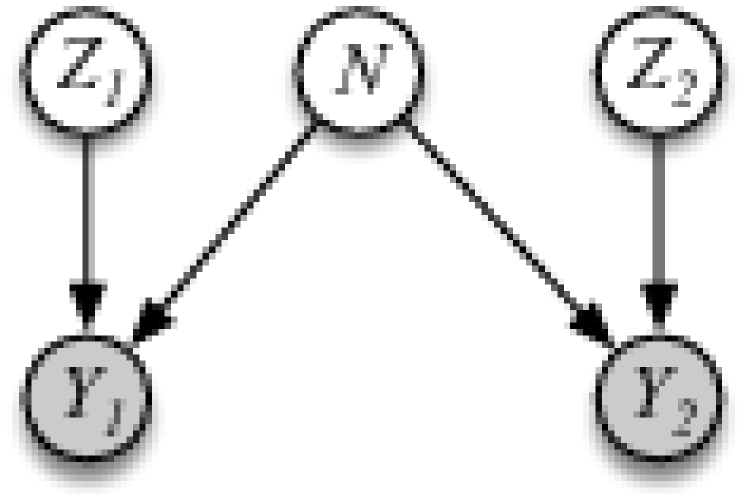
The model motivating half-sibling regression is shown in Figure 1(a). Here, $Z_{1}$ and $Z_{2}$ are two quantities of interest that are known a priori to be independent. In the application of Schölkopf et al. (2015), these are the brightness values of two distant stars. The variables $Y_{1}$ and $Y_{2}$ are measurements of $Z_{1}$ and $Z_{2}$ that are affected by a common noise mechanism $N$, for example, jitter in a telescope. In this model, any dependence between $Y_{1}$ and $Y_{2}$ must be introduced by the noise mechanism. The goal of half-sibling regression is to estimate one target value $Z_{1}$. It does so using the estimator

$$\hat{Z}_{1}=Y_{1}-\mathbb{E}[Y_{1}\mid Y_{2}]$$

which has the interpretation of subtracting from $Y_{1}$ the portion of $Y_{1}$ that can be predicted by $Y_{2}$. In practice, $Y_{2}$ may be vector valued (e.g., the brightness measurements of many other stars), and the graphical model need not follow the exact form given in Figure 1(a) as long as $Y_{2}\bot\!\!\!\!\bot Z_{1}$ but $Y_{2}$ is not independent of $Y_{1}$ given $N$, so that $Y_{2}$ contains some “signature” of the noise process that produces $Y_{1}$ from $Z_{1}$.

2.1 Throwing out the Baby with the Bathwater

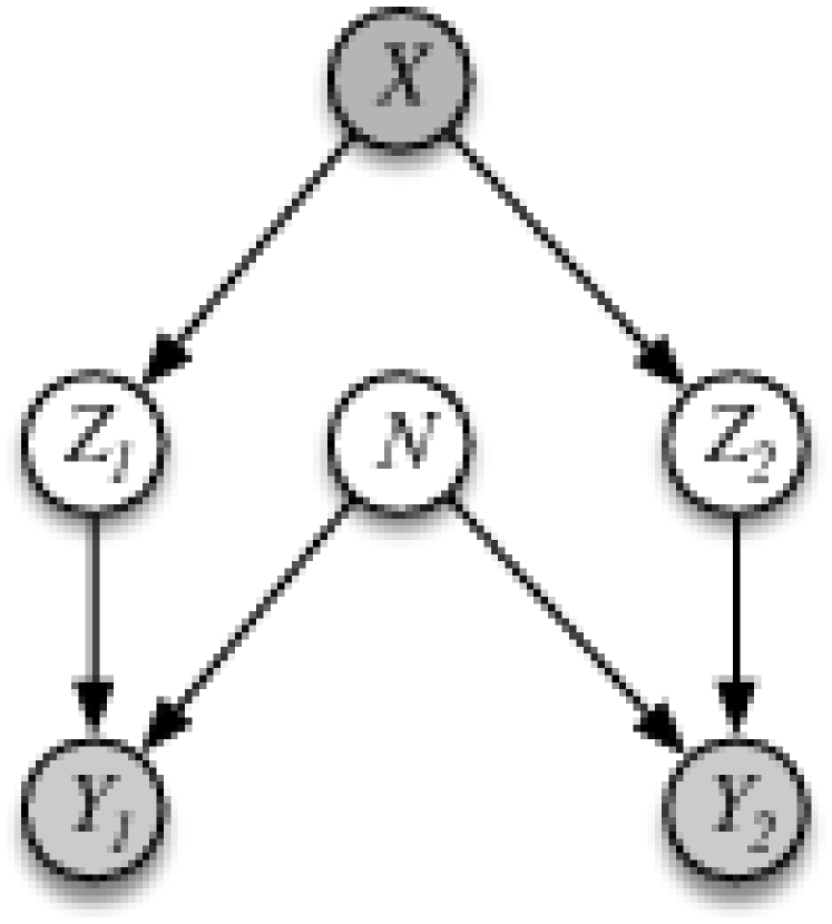
The key limitation of half-sibling regression for our purposes occurs when $Z_{1}$ and $Z_{2}$ are not independent a priori, for example, due to a common cause. In our application $Z_{1}$ and $Z_{2}$ will represent the counts of different species in a survey area, which are affected by common factors such as the habitat and time of year (see Fig. 1). In this setting, $N$ represents factors that affect detectability and are shared across species. In our moth example, moon brightness is key factor, which induces a second source of dependence between moth counts. More generally, $N$ may include transient factors such as weather, or observer attributes such as skill.

If $Z_{1}$ is not independent of $Z_{2}$, there are two sources of dependence between $Y_{1}$ and $Y_{2}$: (1) the a priori dependence induced by $Z_{1}$ and $Z_{2}$, and (2) the dependence introduced by the common noise mechanism $N$. If half-sibling regression is applied in this case, the correction term $\mathbb{E}[Y_{1}\mid Y_{2}]$ will remove some of the true signal, or, as described by Schölkopf et al. (2015), it will throw out (some of) the baby with the bathwater. The variable $Y_{2}$ contains information about the noise mechanism, but it is unclear whether or how this can be teased apart from the a priori dependence.

3 Three-Quarter Sibling Regression

We consider the model shown in Figure 1(b). This extends half-sibling regression by adding the observed variable $X$, which is causal for both $Z_{1}$ and $Z_{2}$. We call $X$ the process covariates. A key assumption of this model is that $Z_{1}\bot\!\!\!\!\bot Z_{2}|X$. This implies two things. First, there is no direct causal link between $Z_{1}$ and $Z_{2}$, which is appropriate for most species pairs in our application to ecological surveys. Second, there are no unobserved common causes of $Z_{1}$ and $Z_{2}$. It is up to the modeler to judge the validity of this assumption, which is standard in causal modeling. In our moth survey application, time-of-year will be the single process covariate, and it is reasonable to assume that there are no other common causes.

In this model, $Y_{1}$ and $Y_{2}$ are now “three-quarter” siblings: they share one parent and their unshared parents are siblings. Mathematically, the key assumption is $Z_{1}\bot\!\!\!\!\bot Y_{2}\mid X$. One of our results will also require $N\bot\!\!\!\!\bot X$. Again, although we are motivated by the particular generative model of Figure 1(b), the method applies to any model that meets these assumptions. For example, the symmetry of the model and presence of $Z_{2}$ is not required — $Y_{2}$ can be any variable that contains some information about the noise mechanism and is conditionally independent of $Z_{1}$ given $X$.

3.1 Estimator

The “three-quarter sibling regression” estimator or 3QS-estimator is:

$$\hat{Z}_{1}=Y_{1}-\mathbb{E}\big{[}\underbrace{Y_{1}-\mathbb{E}[Y_{1}\mid X]}_{\text{residual}}\bigm{|}X,Y_{2}\big{]}$$ (1)

This is equal to $Y_{1}$ minus a correction term. The quantity $Y_{1}-\mathbb{E}[Y_{1}\mid X]$ is the residual after predicting $Y_{1}$ using $X$ alone. This residual is partly due to intrinsic variability in $p(Z_{1}\mid X)$, which we want to preserve, and partly due to the effect of noise when producing the measurement $Y_{1}$. The variables $X$ and $Y_{2}$ should not be predictive of the intrinsic variability but may be predictive of the measurement noise. We subtract the portion of the residual that can be predicted using $X$ and $Y_{2}$ in order to correct $Y_{1}$ towards $Z_{1}$.

Next we prove some results for 3QS analogous to ones in Schölkopf et al. (2015). Under the model of Figure 1(b) and an additional mild assumption, the 3QS-estimator more accurately approximates $Z_{1}$ than $Y_{1}$ does.

Theorem 1.

Assume $Z_{1}\bot\!\!\!\!\bot Y_{2}\mid X$ and $\mathbb{E}[Y_{1}\mid X]=\mathbb{E}[Z_{1}\mid X]$. Then

$$\mathbb{E}\big{[}(\hat{Z}_{1}-Z_{1})^{2}\big{]}\leq\mathbb{E}\big{[}(Y_{1}-Z_{1})^{2}\big{]}.$$

The additional assumption that $\mathbb{E}[Z_{1}\mid X]=\mathbb{E}[Y_{1}\mid X]$ is satisfied by an additive zero-mean noise model, as well other models. Note that this result does not require $N\bot\!\!\!\!\bot X$, as implied by Figure 1(b). Before proving the theorem, we give an alternative expression for $\hat{Z}_{1}$ that is useful for analysis.

Lemma 1.

An equivalent expression for $\hat{Z}_{1}$ is

$$\hat{Z}_{1}=Y_{1}-\mathbb{E}[Y_{1}\mid X,Y_{2}]+\mathbb{E}[Y_{1}\mid X]$$ (2)

Proof.

From Eq. (1) we have

$$\hat{Z}_{1} =Y_{1}-\mathbb{E}\big{[}Y_{1}-\mathbb{E}[Y_{1}\mid X]\bigm{|}X,Y_{2}\big{]}$$

$$=Y_{1}-\mathbb{E}[Y_{1}\mid X,Y_{2}]+\mathbb{E}\big{[}\mathbb{E}[Y_{1}\mid X]\bigm{|}X,Y_{2}\big{]}$$

$$=Y_{1}-\mathbb{E}[Y_{1}\mid X,Y_{2}]+\mathbb{E}[Y_{1}\mid X]$$

The last line holds because $\mathbb{E}[Y_{1}\mid X]$ is a deterministic function of $(X,Y_{2})$. For any random variable $U$ and deterministic function $g$ it is the case that $\mathbb{E}[g(U)\mid U]=g(U)$. ∎

Proof of Theorem 1.

First, note that $\mathbb{E}[Y_{1}\mid X]=\mathbb{E}[Z_{1}\mid X]$ implies $\mathbb{E}[Y_{1}]=\mathbb{E}[Z_{1}]$. Then

$$\mathbb{E}\Big{[} \big{(}Z_{1}-{Y}_{1}\big{)}^{2}\Big{]}$$

$$=\mathbb{E}\Big{[}\big{(}(Z_{1}-\mathbb{E}Z_{1}\big{)}-(Y_{1}-\mathbb{E}Y_{1})\big{)}^{2}\Big{]}$$ (3)

$$=\mathbb{E}\Big{[}\big{(}Z_{1}-Y_{1}-\mathbb{E}[Z_{1}-Y_{1}]\big{)}^{2}\Big{]}$$

$$\geq\mathbb{E}\Big{[}\big{(}Z_{1}-Y_{1}-\mathbb{E}[Z_{1}-Y_{1}\mid Y_{2},X]\big{)}^{2}\Big{]}$$ (4)

$$=\mathbb{E}\Big{[}\big{(}Z_{1}-Y_{1}-\mathbb{E}[Z_{1}\mid X]+\mathbb{E}[Y_{1}\mid Y_{2},X]\big{)}^{2}\Big{]}$$ (5)

$$=\mathbb{E}\Big{[}\big{(}Z_{1}-(Y_{1}-\mathbb{E}[Y_{1}\mid Y_{2},X]+\mathbb{E}[Y_{1}\mid X])\big{)}^{2}\Big{]}$$ (6)

$$=\mathbb{E}\Big{[}\big{(}Z_{1}-\hat{Z}_{1}\big{)}^{2}\Big{]}$$

In Eq. (3), we subtracted $\mathbb{E}Z_{1}$ and added $\mathbb{E}Y_{1}$, which are equal. In Eq. (4), we used the fact that conditional variance is no more than total variance. In Eq. (5), we used the fact that $Z_{1}\bot\!\!\!\!\bot Y_{2}\mid X$. In Eq. (6), we used $\mathbb{E}[Z_{1}\mid X]=\mathbb{E}[Y_{1}\mid X]$ and reordered terms. ∎

3.2 Additive Noise Model

Now, further assume the following additive form for $Y_{1}$:

$$Y_{1}=Z_{1}+f(N).$$ (7)

Here $Z_{1}$ is the “true” value and $f(N)$ an additive error term due to $N$. More generally, we could have $Y_{1}=\phi(Z_{1})+f(N)$ where $\phi$ is an unknown transformation. Since we can never learn such a transformation from observations of $Y_{1}$, we assume the form in Eq. (7), which amounts to reconstructing the hidden variable after transforming it to the same units as $Y_{1}$.

Under the additive noise model, it is possible to quantify the error of the 3QS-estimator for reconstructing $Z_{1}$.

Theorem 2.

Assume $Z_{1}\bot\!\!\!\!\bot Y_{2}\mid X$ and $N\bot\!\!\!\!\bot X$. Under the additive model of Eq. (7), we have

$$\mathbb{E}\big{[}\big{(}\hat{Z}_{1}-(Z_{1}+\mathbb{E}[f(N)])\big{)}^{2}\big{]}=\operatorname{Var}\big{[}f(N)\mid X,Y_{2}\big{]}.$$

Proof.

$$\hat{Z}_{1} =Y_{1}-\mathbb{E}[Y_{1}\mid X,Y_{2}]+\mathbb{E}[Y_{1}\mid X]$$

$$\begin{aligned} =Z_{1}&+f(N)-\big{(}\mathbb{E}[Z_{1}|X,Y_{2}]+\mathbb{E}[f(N)|X,Y_{2}]\big{)}\\ &+\big{(}\mathbb{E}[Z_{1}\mid X]+\mathbb{E}[f(N)\mid X]\big{)}\end{aligned}$$ (8)

$$\begin{aligned} =Z_{1}&+f(N)-\big{(}\mathbb{E}[Z_{1}|X]+\mathbb{E}[f(N)|X,Y_{2}]\big{)}\\ &+\big{(}\mathbb{E}[Z_{1}\mid X]+\mathbb{E}[f(N)]\big{)}\end{aligned}$$ (9)

$$=Z_{1}+\big{(}f(N)-\mathbb{E}[f(N)\mid X,Y_{2}]\big{)}+\mathbb{E}[f(N)]$$ (10)

Eq. (8) uses the additive expansion of $Y_{1}$ three times. Eq. (9) uses the facts that $Z_{1}\bot\!\!\!\!\bot Y_{2}\mid X$ and $N\bot\!\!\!\!\bot X$. Eq. (10) rearranges. Then, rearranging,

$$\hat{Z}_{1}-(Z_{1}+\mathbb{E}[f(N)])=f(N)-\mathbb{E}[f(N)\mid X,Y_{2}].$$

Therefore,

$$\mathbb{E}\big{[}\big{(}\hat{Z}_{1}\!-\!(Z_{1}\!+\!\mathbb{E}[f(N)])\big{)}^{2} =\mathbb{E}\big{[}\big{(}f(N)\!-\!\mathbb{E}[f(N)|X,Y_{2}]\big{)}^{2}\big{]}$$

$$=\operatorname{Var}[f(N)\mid X,Y_{2}].$$

∎

Theorem 2 says that it is possible to reconstruct $Z_{1}$—up to a constant additive offset equal to the mean of the measurement error—with squared error equal to the conditional variance of the measurement error given the observed variables $X$ and $Y_{2}$. If the measurement error is completely determined by the observed variables, then $Z_{1}+\mathbb{E}[f(N)]$ is reconstructed exactly.

Corollary 1.

If there is a function $\psi$ such that $f(N)=\psi(X,Y_{2})$, then $\hat{Z}_{1}=Z_{1}+\mathbb{E}[f(N)]$.

Proof.

In this case $\operatorname{Var}\big{[}f(N)\bigm{|}X,Y_{2}\big{]}=\operatorname{Var}\big{[}\psi(X,Y_{2})\bigm{|}X,Y_{2}\big{]}=0$, which implies that $\hat{Z}_{1}\!-(Z_{1}+\mathbb{E}[f(N)])=0$. ∎

3.2.1 Implementation

In practice, the conditional expectations in the 3QS-estimator are unknown, but can be replaced by regression models. The 3QS-estimator used in practice is:

$$\hat{Z}_{1}=Y_{1}-\hat{\mathbb{E}}\big{[}Y_{1}-\hat{\mathbb{E}}[Y_{1}\mid X]\bigm{|}X,Y_{2}\big{]}$$

where $\hat{\mathbb{E}}[B\mid A]$ is a regression model trained to predict $B$ from $A$.

In our application, the $Y_{i}$ variables are symmetric and represent counts of different species. We first fit a regression model $\hat{\mathbb{E}}[Y_{i}\mid X]$ using only process covariates for each species. Then, define $R_{i}=Y_{i}-\hat{\mathbb{E}}[Y_{i}\mid X]$ to be the residual for species $i$, and let $R_{-i}$ be the vector of residuals for all other species. We use the estimator

$$\hat{Z}_{i}=Y_{i}-\hat{\mathbb{E}}\big{[}R_{i}\mid R_{-i}].$$

This has a very simple interpretation. We subtract the portion of the residual for the target species that can be predicted using the residuals of the other species. This is a special case of the 3QS-estimator where the regression model using $(X,Y_{-i})$ as predictors is parameterized as a function of only the residual $Y_{-i}-\hat{\mathbb{E}}[Y_{-i}\mid X]$.

4 Experiments

In this section we experimentally demonstrate the ability of 3QS-regression to remove systematic measurement error in the presence of common causes using first synthetic data and then a moth survey data set from the Discover Life project.

4.1 Synthetic Experiments

(a)

(b)

(c)

(d)

Figure 2: Results on synthetic data. (a) MSE vs species count $n$, (b) MSE vs noise deviation $\sigma_{\epsilon}$, (c) HS and 3QS MSE vs. $n$, (d) HS and 3QS MSE vs. $\sigma_{\epsilon}$.

We first conducts experiments using synthetic data, for which the true value of $Z_{1}$ is known. This allows us to measure the ability of 3QS-regression to recover $Z_{1}$ and evaluate its performance in settings where the auxiliary measurements $Y_{2}=Y_{-1}$ contain a varying amount of information about the noise mechanism.

4.1.1 Methodology

Our synthetic data generation is patterned off the experiments of Schölkopf et al. (2015) for half-sibling regression, but extended to include process covariates. We simulated $n$ species (indexed by $i$) whose occurrences $Y_{i}$ are determined as the following function of a process covariate $X\in\mathbb{R}$ and noise variable $N\in\mathbb{R}$:

$$Y_{i}=\underbrace{w^{(i)}_{X}X}_{Z_{i}}+\underbrace{g_{i}(w^{(i)}_{N}N)}_{f_{i}(N)}+\epsilon.$$

The coefficients $w^{(i)}_{X}$ and $w^{(i)}_{N}$ are drawn uniformly from $[-1,1]$ for each species, and control the relationship between the species occurrence and the process and noise variables. The function $g_{i}$ is a sigmoid function with randomized parameters (to control the inflection points, etc.). Finally $\epsilon\sim\mathcal{N}(0,\sigma^{2}_{\epsilon})$ is independent noise.

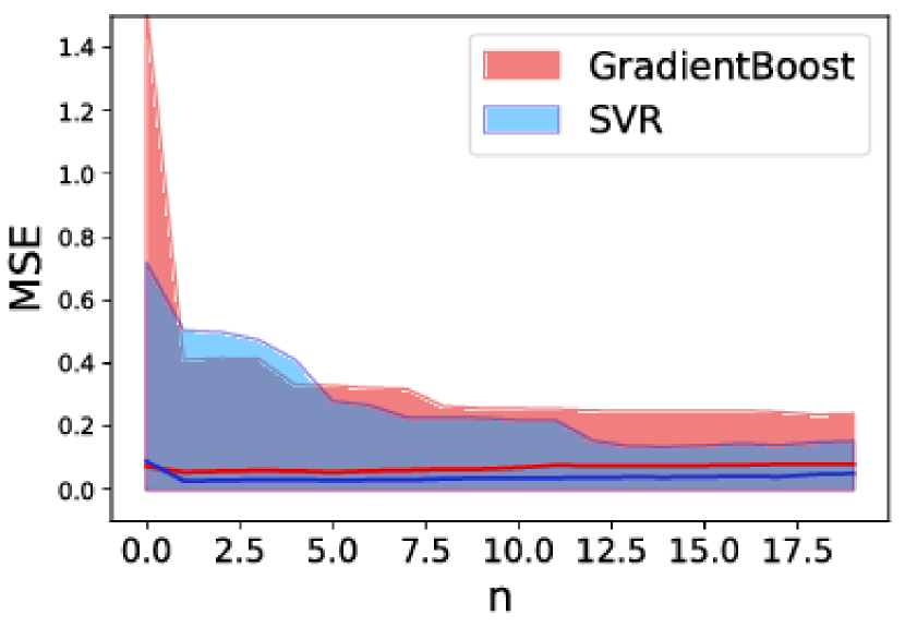
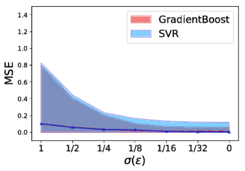
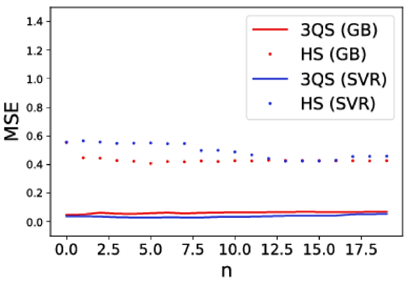
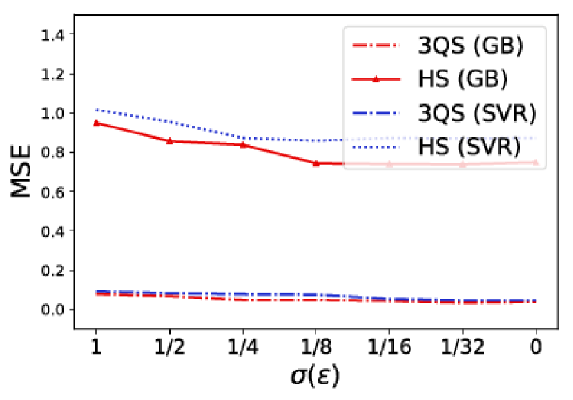
We conduct two experiments to simulate decreasing the uncertainty about $f_{1}(N)$ given $Y_{-1}$. In the first case we set $\sigma^{2}_{\epsilon}=0$ and increase the number of species, each with its own noise function $f_{i}$. As the number of species $n$ increases, we get more predictors of the error $f_{1}(N)$. In the second experiment we fix $n=2$ and $f_{1}=f_{2}$ (i.e the effect of noise on both species is exactly the same) while varying the noise $\sigma^{2}_{\epsilon}$. In either case, when the conditional variance of $f_{1}(N)$ given $(X,Y_{-1})$ reduces, Theorem 2 predicts a more accurate reconstruction.

For these experiments we used the alternate form of the estimator given in Eq. 2, which means we fit regression models $\hat{\mathbb{E}}[Y_{i}|X,Y_{-i}]$ and $\hat{\mathbb{E}}[Y_{i}|X]$ and computed $\hat{Z}_{i}$ according to Eq. 2. The estimators could be shifted from $Z_{i}$ by any constant offset (cf. Theorem 2), so we centered them to have zero-mean to match $Z_{i}$. We conduct our experiments with two different regression algorithms—support-vector regression (SVR) and gradient boosted regression trees, using implementations and default settings from the scikit-learn package. Following Schölkopf et al. (2015), we create 20 different fixed instances and measure the mean squared error (MSE) of our denoised counts $\hat{Z}_{i}$ against true value $Z_{i}$.

Results.

Figures  2(a) and 2(b) show the reconstruction error as a function of the number of species $n$ and noise variance $\sigma^{2}_{\epsilon}$, respectively. The figures plot mean MSE and error across the runs. Fig. 2(a) shows that increasing the number of species in $Y_{-i}$ causes error to decrease with both regression methods. This is expected, because with more predictors that are correlated with $f(N)$, we can learn a better model for the systematic error. Fig. 2(b) shows that as $\sigma^{2}_{\epsilon}\to 0$ the error also tends towards zero. This is also expected, because, in this case, $f(N)$ becomes a deterministic function of $X,Y_{2}$. Figs. 2(c) and 2(d) compare the mean MSE of half-sibling (HS) regression against our method (3QS). HS regression performs poorly due to the common dependence of $Y_{i}$ variables on $X$.

4.2 Discover Life Moth Observations

Figure 3: Residuals and moon brightness vs. time. Residuals are calculated relative to a predictive model fit across several years.

Figure 4: Pairwise scatter plots of residuals for common species and moon brightness. Inset numbers are correlations.

Our second set of experiments use moth survey data from the Discover Life project for studying spatio-temporal variation in moth communities. This dataset consists of counts of moths of different species collected at regular intervals at different study sites by both citizen scientists and moth experts. The protocol involves using artificial light to attract moths to a white surface and then photographing and identifying each specimen. The dataset spans eight years and has been used for analysing seasonal flights Pickering (2015), comparative taxonomy Pickering et al. (2016) and other studies. The data set is unique in its temporal resolution—at some of the sites, counts have been conducted almost every day for many years.

A typical use of this type of data is to estimate smooth curves of species abundance versus time such as the ones shown in Fig. 1 (see also Dennis et al. (2013)). The smooth curve is then used as a proxy of the actual abundance at a given site in a given year to create indices of population size and to analyze temporal patterns, such as the timing of different generations (many species occur in discrete generations each year, e.g., see H. fucosa in Fig. 1). Scientists are especially interested in how populations and timing vary across years to understand population dynamics and potential links with external factors such as climate.

4.2.1 Moon Brightness

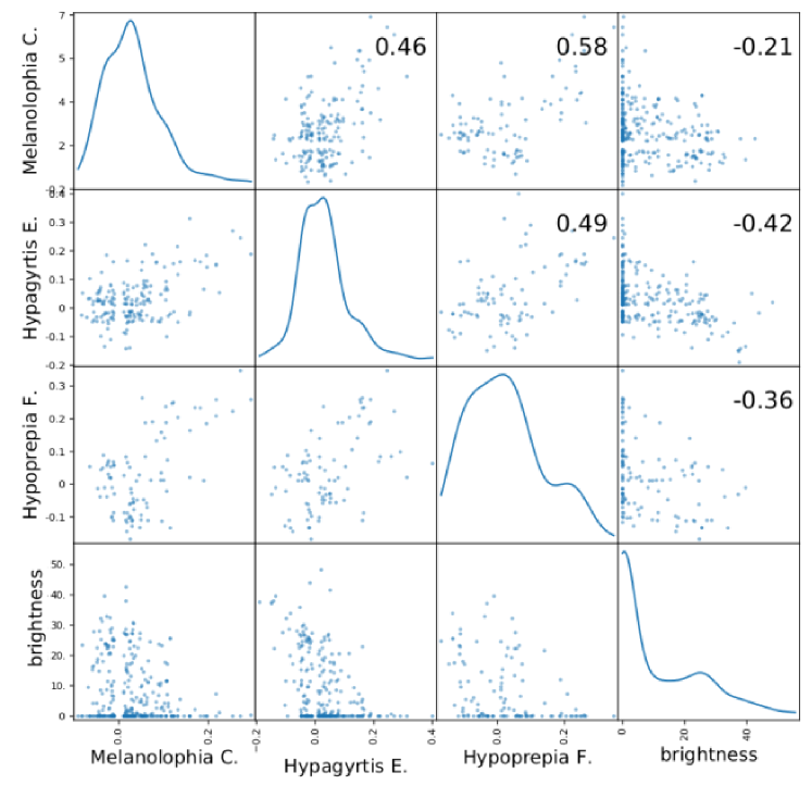
A known systematic bias in moth counting studies is lunar brightness. On nights when the moon is bright, moths are less likely to be attracted to the white surface where they are photographed and counted. We show evidence of this in Figs. 3 and 4. Fig. 3 shows the residuals of moth counts with respect to a fitted model of count vs. day-of-year, together with moon brightness. The residuals track the moon phases and are anti-correlated with moon brightness. For example notice the significantly positive residual during early September which seems to rise exactly as lunar brightness reaches its nadir. Fig. 4 shows pairwise scatter plots and correlation values for the residuals of three moth species together with moon brightness. All residuals are negatively correlated with moon brightness, and positively correlated with each other, with moon brightness being one contributing factor. In this example residuals are generally more correlated with each other than with moon brightness. One explanation is that moon brightness is measured using astronomical calculations and does not correspond exactly to brightness on the ground, which depends on factors like cloud cover. A second explanation is the effect of other factors besides brightness on detectability. A third (and less desirable) explanation is that there are other causal factors that are unmeasured. The reality is likely some combination of the three.

4.2.2 Overall Experimental Strategy

Our hypothesis is that moon brightness is one source of systematic measurement error that can be effectively detected and removed using 3QS-regression. To test this, we will use moon brightness as an external variable that is not available to our methods, and test the correlation of moth counts with brightness before and after applying denoising techniques, as well as the accuracy of predictive models on “gold-standard” test nights when lunar brightness is minimal, so this particular source of variability is removed.

Our overall goal is to develop the best smoothed models of abundance over time for individual years (cf. Fig. 1), and we hypothesize that correcting systematic errors will help. Evaluation is challenging because the true abundance in a given year is unknown. Our approach will be to fit smooth models in individual years and test their predictive accuracy for other years. It is not our hope that the predictive accuracy is perfect — indeed, we want our model to preserve variability across years. However, another source of such variability is differently aligned moon phases, which affect detection but not true abundance. A model that corrects for such systematic errors should therefore generalize better to other years by reducing this source of variation.

4.2.3 Methodology

We choose moth counts from one site (Blue Heron Drive) for 2013 through 2018. Lunar brightness for the time of observation is computed with the software Pyephem using the latitude and longitude of the site. We use the log-transformed counts of the most common 10 species.

We hold out one year at a time for testing and make predictions using each other year, for a total of $20$ train-year / test-year pairs. When predicting one test year, we first use all four other years to fit the regression models $\hat{\mathbb{E}}[Y_{i}|X]$ and $\hat{\mathbb{E}}[R_{i}|R_{-i}]$ where $R_{i}=Y_{i}-\hat{\mathbb{E}}[Y_{i}|X]$ is the residual. In all experiments, $X$ consists only of day-of-year. We then compute $\hat{Z}_{i}$ for each training year using the 3QS-estimator, fit a smoothed regression model $\hat{\mathbb{E}}[\hat{Z}_{i}|X]$ to the denoised counts for a single training year at a time, and use the model to predict on the test year. This is repeated for all train-year / test-year pairs and for all species. We compare 3QS-regression to multiple baselines, including using the original measurements $Y_{1}$ to estimate $Z_{1}$, as well as the half-sibling (HS) regression method of Schölkopf et al. (2015). The pyGAM package  Servén and Brummitt (2018) for generalized additive models (GAMs) is used in all regression models.

	Correlation with MB			Std. dev. %
Species	$Y$	$\hat{Z}_{\text{HS}}$	$\hat{Z}_{\text{3QS}}$	$\hat{Z}_{\text{HS}}$	$\hat{Z}_{\text{3QS}}$
Halysidota H.	-0.20	-0.14	-0.16	0.91	0.96
Hypoprepia F.	-0.15	-0.01	-0.04	0.80	0.90
Hypagyrtis E.	-0.18	-0.09	-0.11	0.82	0.95
Microcrambus E.	-0.16	-0.03	-0.10	0.84	0.97
Clemensia A.	-0.13	-0.09	-0.05	0.92	0.95
Lochmaeus B.	-0.13	-0.01	-0.05	0.82	0.92
Melanolophia C.	-0.29	-0.22	-0.20	0.77	0.88
Iridopsis D.	-0.18	-0.15	-0.13	0.94	0.97

Table 1: Correlation with lunar brightness before and after denoising, and retained standard deviation as a fraction of that of $Y$

(a)

(b)

Figure 5: Average percent improvement in predictive MSE relative to a GAM fitted to the raw counts. (a) Different estimators. (b) 3QS with increasing number of species.

Results: Moon Brightness.

We first compare the relationship between counts and moon brightness before and after 3QS-regression. It is expected that most species will have negative correlation with lunar brightness initially, but the correlation will be significantly less after denoising. The results are presented in Table 1. Typical correlations between raw counts and lunar brightness are on the order of -15% to -20%; after denosing, the magnitude of correlations decrease by an average of about 7%. The HS-regression estimator is shown for comparison, and also decorrelates the counts from lunar brightness. However if counts are correlated due to a common cause, HS-regression will also remove some of the intrinsic (non-noise) variability (the “throwing out the baby with the bathwater” problem). This can also be seen in Table 1: the overall variance of $\hat{Z}_{\text{HS}}$ is significantly reduced relative to the raw counts. We will show in our next experiment this removed variance corresponds to true variability that should not be removed.

Results: Predictive Accuracy.

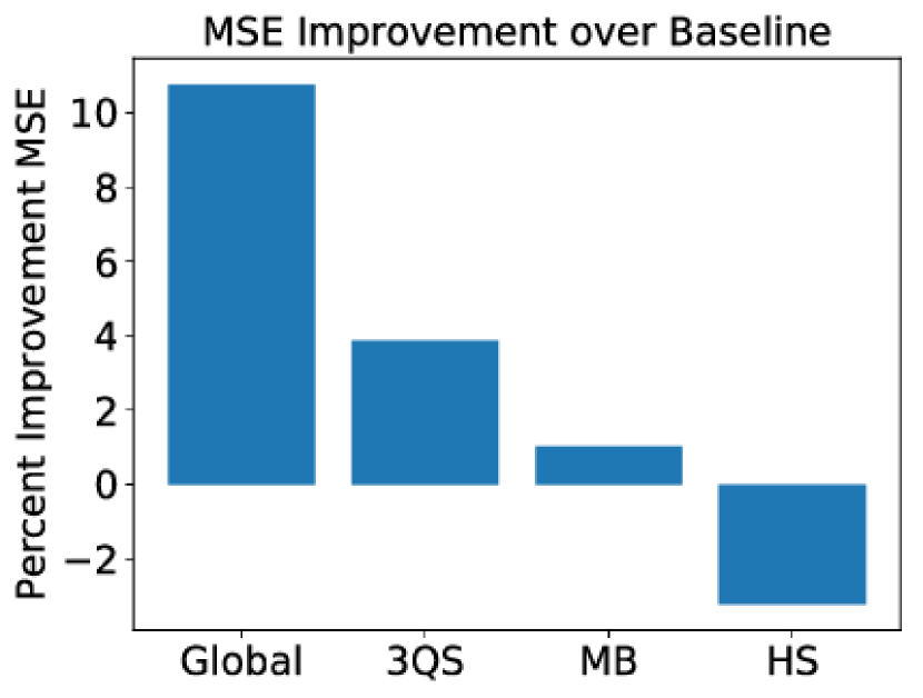
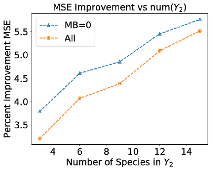
Fig. 5(a) shows predictive accuracy of several methods averaged over all species and train-year / test-year pairs. The numbers are percent improvement in MSE relative to the baseline of a GAM fit to the noisy counts in the training year. MSE is computed only on data from the test-year with moon brightness zero. “Global” is an oracle model shown for comparison. It is trained on raw counts of four training years instead of one. By fitting one model to multiple training years, it is expected to smooth out both sources of year-to-year variability (intrinsic and moon phase) and therefore predict better on a held-out year. However, this is not our modeling goal — we want to preserve intrinsic year-to-year variability and eliminate variability due to moon phase. “MB” is a model that includes moon brightness as a feature to model detection variability. The results show that 3QS outperforms all competitors, including the MB model that has access to moon brightness as a feature. The global model performs better, as expected. The HS model is worse than the baseline due to removing intrinsic variability. Fig. 5(b) shows the impact of using a greater number of species for $Y_{2}$. MSE is reported for the full test set as well as the moon-brightness zero set. By Theorem 2, we expect more species to reduce the conditional variance and therefore improve accuracy, which is borne out in Fig. 5(b) on both test-sets. Accuracy on the full test set is worse than on the moon-brightness zero test set, which is expected due to extra variability in the test set.

5 Conclusion

Building on recent work on causal models, we presented three-quarter-sibling (3QS) regression to remove systematic measurement error for species that share observed common causes. We theoretically analyzed 3QS and presented empirical evidence of its success. A future line of work would be to use simultaneous measurements to quantify uncertainty, possibly combined with Bayesian methods Ellison (2004). Our method may also be useful applied to other domains, such as under-reporting of drug use Adams et al. (2019). A final question would be to address confounding in the presence of non-independent noise, i.e., when $X$ is not independent of $N$.

References

- Adams et al. [2019] Roy Adams, Yuelong Ji, Xiaobin Wang, and Suchi Saria. Learning models from data with measurement error: Tackling underreporting. arXiv preprint arXiv:1901.09060, pages 1–8, 2019.
- Dail and Madsen [2011] David Dail and Lisa Madsen. Models for estimating abundance from repeated counts of an open metapopulation. Biometrics, 67(2):577–87, 2011.
- Dennis et al. [2013] Emily B. Dennis, Stephen N. Freeman, Tom Brereton, and David B. Roy. Indexing butterfly abundance whilst accounting for missing counts and variability in seasonal pattern. Methods in Ecology and Evolution, 4(7):637–645, 2013.
- Ellison [2004] Aaron Ellison. Bayesian inference in ecology. Ecology Letters, 7(6):509–52, 2004.
- Frénay and Verleysen [2014] Benoît Frénay and Michel Verleysen. Classification in the presence of label noise: a survey. IEEE transactions on neural networks and learning systems, 25(5):845–869, 2014.
- Hutchinson et al. [2017] Rebecca A. Hutchinson, Liqiang He, and Sarah C Emerson. Species distribution modeling of citizen science data as a classification problem with class-conditional noise. In AAAI, pages 4516–4523, 2017.
- Kelling et al. [2015] Steve Kelling, Alison Johnston, Wesley M Hochachka, Marshall Iliff, Daniel Fink, Jeff Gerbracht, Carl Lagoze, Frank A La Sorte, Travis Moore, Andrea Wiggins, et al. Can observation skills of citizen scientists be estimated using species accumulation curves? PLoS One, 10(10):e0139600, 2015.
- Knape and Korner-Nievergelt [2015] Jonas Knape and Fränzi Korner-Nievergelt. Estimates from non-replicated population surveys rely on critical assumptions. Methods in Ecology and Evolution, 6(3):298–306, 2015.
- Knape and Korner-Nievergelt [2016] Jonas Knape and Fränzi Korner-Nievergelt. On assumptions behind estimates of abundance from counts at multiple sites. Methods in Ecology and Evolution, 7(2):206–209, 2016.
- Lele et al. [2012] Subhash R. Lele, Monica Moreno, and Erin Bayne. Dealing with detection error in site occupancy surveys: what can we do with a single survey? Journal of Plant Ecology, 5(1):22–31, 2012.
- MacKenzie et al. [2002] Darryl I. MacKenzie, James D. Nichols, Gideon B. Lachman, Sam Droege, Andrew Royle, and Catherine A. Langtimm. Estimating site occupancy rates when detection probabilities are less than one. Ecology, 83(8):2248–2255, 2002.
- Nettleton et al. [2010] David F. Nettleton, Albert Orriols-Puig, and Albert Fornells. A study of the effect of different types of noise on the precision of supervised learning techniques. Artificial intelligence review, 33(4):275–306, 2010.
- Pickering et al. [2016] John Pickering, Dorothy Madamba, Tori Staples, and Rebecca Walcott. Status of moth diversity and taxonomy: a comparison between Africa and North America north of Mexico. S. Lep. News, 38(3):241–248, 2016.
- Pickering [2015] John Pickering. Why fly now? Pupa banks, aposematism, and other factors that may explain observed moth flight activity. S. Lep. News, 38(1):67–72, 2015.
- Royle [2004] J. Andrew Royle. N-mixture models for estimating population size from spatially replicated counts. Biometrics, 60(1):108–115, 2004.
- Schölkopf et al. [2015] Bernhard Schölkopf, David Hogg, Dun Wang, Dan Foreman-Mackey, Dominik Janzing, Carl-Johann Simon-Gabriel, and Jonas Peters. Removing systematic errors for exoplanet search via latent causes. In Proceedings of the 32nd International Conference on Machine Learning (ICML), pages 2218–2226. PMLR, 2015.
- Servén and Brummitt [2018] Daniel Servén and Charlie Brummitt. pyGAM: Generalized additive models in Python, March 2018.
- Sólymos and Lele [2016] Péter Sólymos and Subhash R. Lele. Revisiting resource selection probability functions and single-visit methods: clarification and extensions. Methods in Ecology and Evolution, 7(2):196–205, 2016.
- Yu et al. [2010] Jun Yu, Weng-Keen Wong, and Rebecca A. Hutchinson. Modeling experts and novices in citizen science data for species distribution modeling. In 2010 IEEE International Conference on Data Mining (ICDM), pages 1157–1162. IEEE, 2010.
- Yu et al. [2014a] Jun Yu, Rebecca A. Hutchinson, and Weng-Keen Wong. A latent variable model for discovering bird species commonly misidentified by citizen scientists. In Twenty-Eighth AAAI Conference on Artificial Intelligence, 2014.
- Yu et al. [2014b] Jun Yu, Weng-Keen Wong, and Steve Kelling. Clustering species accumulation curves to identify skill levels of citizen scientists participating in the eBird project. In Twenty-Sixth IAAI Conference, 2014.