The Query Complexity of Local Search and Brouwer in Rounds

Abstract

We consider the query complexity of finding a local minimum of a function defined on a graph, where at most $k$ rounds of interaction with the oracle are allowed. Rounds model parallel settings, where each query takes resources to complete and is executed on a separate processor. Thus the query complexity in $k$ rounds informs how many processors are needed to achieve a parallel time of $k$.

We focus on the $d$-dimensional grid $\{1,2,\ldots,n\}^{d}$, where the dimension $d\geq$ is a constant, and consider two regimes for the number of rounds: constant and polynomial in $n$. We give algorithms and lower bounds that characterize the trade-off between the number of rounds of adaptivity and the query complexity of local search.

When the number of rounds $k$ is constant, the query complexity of local search in $k$ rounds is $\Theta\bigl{(}n^{\frac{d^{k+1}-d^{k}}{d^{k}-1}}\bigl{)}$, for both deterministic and randomized algorithms.

When the number of rounds is polynomial, i.e. $k=n^{\alpha}$ for $0<\alpha<d/2$, the randomized query complexity is $\Theta\left(n^{d-1-\frac{d-2}{d}\alpha}\right)$ for all $d\geq 5$. For $d=3$ and $d=4$, we show the same upper bound expression holds and give almost matching lower bounds.

The local search analysis also enables us to characterize the query complexity of computing a Brouwer fixed point in rounds. Our proof technique for lower bounding the query complexity in rounds may be of independent interest as an alternative to the classical relational adversary method of Aaronson [Aar06] from the fully adaptive setting.

1 Introduction

Local search is a powerful heuristic embedded in many natural processes and often used to solve hard optimization problems. Examples of local search algorithms include the Lin–Kernighan algorithm for the traveling salesman problem, the Metropolis-Hastings algorithm for sampling, and the WalkSAT algorithm for Boolean satisfiability. Johnson, Papadimitriou, and Yannakakis [JPY88] introduced the complexity class PLS to capture local search problems for which local optimality can be verified in polynomial time. Natural PLS complete problems include finding a pure Nash equilibrium in a congestion game [FPT04] and a locally optimum maximum cut in a graph [SY91].

In the query complexity model, we are given a graph $G=(V,E)$ and oracle access to a function $f:V\to\mathbb{R}$. The set $V$ can represent any universe of elements with a notion of neighbourhood and the goal is to find a vertex $v$ that satisfies the local minimum property: $f(v)\leq f(u)$ for all $(u,v)\in E$. The query complexity is the number of oracle queries needed to find a local minimum in the worst case. Upper bounds on the complexity of local search can suggest improved algorithms for problems such as finding pure Nash equilibria in congestion games. On the other hand, local search lower bounds can translate into bounds for computing stationary points [BM20], thus giving insights into the runtime of algorithms such as gradient descent.

The query complexity of local search was first considered by Aldous [Ald83], who showed that steepest descent with a warm start is a good randomized algorithm: first query $t$ vertices $x_{1},\ldots,x_{t}$ selected uniformly at random and pick the vertex $x^{*}$ that minimizes the function among these . Then run steepest descent from $x^{*}$ and stop when no further improvement can be made, returning the final vertex reached. When $t=\sqrt{nd}$, where $n$ is the number of vertices and $d$ the maximum degree in the graph $G$, the algorithm issues $O(\sqrt{nd})$ queries in expectation and has roughly as many rounds of interaction with the oracle.

Multiple rounds of interaction can be expensive in applications. For example, when algorithms such as gradient descent are run on data stored in the cloud, there can be delays due to back and forth messaging across the network. A remedy for such delays is designing protocols with fewer rounds of communication. Aldous’ algorithm described above is highly sequential, i.e. requires many rounds of interaction with the oracle, even though its total query complexity is essentially optimal for graphs such as the hypercube and the $d$-dimensional grid [Ald83, SY09, Zha09].

We consider the query complexity of local search in $k$ rounds, where an algorithm asks a set of queries in each round, then receives the answers, after which it issues the set of queries for the next round. This setting also captures parallel computation, since it can model a central machine that issues in each round $i$ a set of queries, one to each processor, then waits for the answers before issuing the next set of parallel queries in round $i+1$. The question then is how many processors are needed to achieve a parallel search time of $k$, or equivalently, what is the query complexity in $k$ rounds.

Parallel complexity is a fundamental concept, which was studied extensively for problems such as sorting, selection, finding the maximum, and sorted top-$k$ [Val75, Pip87, Bol88, AAV86, WZ99, GGK03b, BMW16, BMP19, CMM20]. An overview on parallel sorting algorithms is given in the book by Akl [Akl14]. Nemirovski [Nem94] considered the parallel complexity of optimization, which was analyzed for submodular functions in [BS18]. Bubeck and Mikulincer [BM20] studied algorithms with few rounds (aka low depth) for the problem of computing stationary points.

1.1 Roadmap of the paper

Section 2 discusses related work. Section 3 states the model and our results. Section 4 overviews the results and proof techniques for local search, with references to the appendix for the full proofs. Section 5 overviews the results and proofs for Brouwer.

2 Related Work

The query complexity of local search was studied first experimentally by Tovey [Tov81]. Aldous [Ald83] gave the first theoretical analysis of local search, showing an upper bound of $O(n\cdot 2^{n/2})$ and a lower bound of $\Omega(2^{n/2-o(n)})$ for the query complexity of randomized algorithms on the $n$-dimensional hypercube. [Ald83] also gave a lower bound construction, which is obtained by considering an initial vertex $v_{0}$ uniformly at random. The function value at $v_{1}$ is $f(v_{0})=0$. From this vertex, start an unbiased random walk $v_{0},v_{1},\ldots$ For each vertex $v$ in the graph, set $f(v)$ equal to the first hitting time of the walk at $v$; that is, $f(v)=min\{t\mid v_{t}=v\}$. The function $f$ defined this way has a unique local minimum at $f(0)$. By analyzing this distribution, [Ald83] showed a lower bound of $2^{n/2-o(n)}$ on the hypercube.

Llewellyn, Tovey, and Trick [LTT93] considered the deterministic query complexity of local search and devised a divide-and-conquer approach, which has higher total query complexity but uses fewer rounds. Their algorithm is deterministic and identifies in the first step a vertex separator $S$ of the input graph $G$ . Afterwards, it queries all the vertices in $S$ to find the minimum $v$ among these. If $v$ is a local minimum of $G$, then return it. Otherwise, there is a neighbour $w$ of $v$ with $f(w)<f(v)$. Repeat the whole procedure on the new graph $G^{\prime}$, defined as the connected component of $G\setminus S$ containing $w$. Correctness holds since the steepest descent from $w$ cannot escape $G^{\prime}$. On the $d$-dimensional grid, the vertex separator $S$ can be defined as the $(d-1)$-dimensional wall that divides the current connected component evenly; thus a local optimum can be found with $O(n^{d-1})$ queries in $O(\log{n})$ rounds.

[LT93, AK93] applied the adversarial argument proposed in [LTT93] to show that $\Omega(n^{d-1})$ queries are necessary for any deterministic algorithm on the $d$-dimensional grid of side length $n$. [LTT93] also studied arbitrary graphs, showing that $O(\sqrt{n}+\delta\log{n})$ queries are sufficient on graphs with $n$ vertices when the maximum degree of the graph is $\delta$ and the graph has constant genus.

We observe the contrast between the randomized algorithm [Ald83], which is almost sequential, running in $O(n^{d/2})$ rounds, and the deterministic divide-and-conquer algorithm [LTT93], which can be implemented in $O(\log{n})$ rounds. Even though the randomized algorithm [Ald83] is (essentially) optimal in terms of number of queries, it takes many rounds and so it cannot be parallelized directly. Thus it is natural to ask whether this algorithm can be parallelized and what is the tradeoff between the total query complexity and the number of rounds.

Aaronson [Aar06] improved the bounds given by Aldous[Ald83] for randomized algorithms by designing a novel technique called the relational adversarial method inspired by the adversarial method in quantum computing. This method avoids analyzing the posterior distribution during the execution directly and gave improved lower bounds for both the hypercube and the grid. Follow-up work by Zhang [Zha09] and Sun and Yao [SY09] obtained even tighter lower bounds for the grid using this method with better choices on the random process; their lower bound is $\widetilde{\Omega}\bigl{(}n^{\frac{d}{2}}\bigr{)}$, which is nearly optimal.

The computational complexity of local search is captured by the class PLS, which was defined by Johnson, Papadimitriou, and Yannakakis [JPY88] to model the difficulty of finding locally optimal solutions to optimization problems. A class related to PLS is PPAD, introduced by Papadimitriou[Pap94] to study the computational complexity of finding a Brouwer fixed-point [Pap94] contains many natural problems that are computationally equivalent to the problem of finding a Brouwer fixed point [CD09], such as finding an approximate Nash equilibrium in a multi-player or two-player game [DGP09, CDT09], an Arrow-Debreu equilibrium in a market [VY11, CPY17], and a local min-max point recently by Daskalakis, Skoulakis, and Zampetakis [DSZ21]. The query complexity of computing an $\epsilon$-approximate Brouwer fixed point was studied in a series of papers for fully adaptive algorithms starting with Hirsch, Papadimitriou, and Vavasis [HPV89], later improved by Chen and Deng [CD05] and Chen and Teng [CT07].

The classes PLS and PPAD are related, both being a subset of TFNP. Fearnley, Goldberg, Hollender, and Savani [FGHS21] showed that the class CLS, introduced by Daskalakis and Papadimitriou [DP11] to capture continuous local search, is equal to PPAD $\cap$ PLS. The query complexity of continuous local search has also been studied (see, e.g., [HY17]).

Valiant [Val75] initiated the study of parallelism using the number of comparisons as a complexity measure and showed that $p$ processor parallelism can offer speedups of at least $O\bigl{(}\frac{p}{\log\log p}\bigr{)}$ for problems such as sorting and finding the maximum of a list of $n>p$ elements.

Nemirovski [Nem94] studied the parallel complexity of optimization, with more recent results on submodular optimization due to Balkanski and Singer [BS18]. An overview on parallel sorting algorithms is given in the book by Akl [Akl14] and many works on sorting and selection in rounds can be found in [Val75, Pip87, Bol88, AAV86, WZ99, GGK03a], aiming to understand the tradeoffs between the number of rounds of interaction and the query complexity.

Another setting of interest where rounds are important is active learning, where there is an “active” learner that can submit queries—taking the form of unlabeled instances—to be annotated by an oracle (e.g., a human) [Set12]. However each round of interaction with the human annotator has a cost, which can be captured through a budget on the number of rounds.

3 Model and Results

In this section we present the model for local search and Brouwer, define the deterministic and randomized query complexity, and summarize our results. The dimension $d$ for both local search and Brouwer fixed-point is a constant. Unless otherwise specified, we have $d\geq 2$.

3.1 Local Search

Let $G=(V,E)$ be an undirected graph and $f:V\rightarrow\mathbb{R}$ a function, where $f(\mathbf{x})$ is the value of node $\mathbf{x}\in V$. We have oracle access to $f$ and the goal is to find a local minimum, that is, a vertex $\mathbf{x}$ with the property that $f(\mathbf{x})\leq f(\mathbf{y})$ for all neighbours $\mathbf{y}$ of $\mathbf{x}$.

We focus on the setting where the graph is a $d$-dimensional grid of side length $n$. Thus $V=[n]^{d}$, where $[n]=\{1,2,\ldots,n\}$ and $(\mathbf{x},\mathbf{y})\in E$ if $\|\mathbf{x}-\mathbf{y}\|_{1}=1$.

The grid is a well-known graph that arises in applications where there is a continuous search space, which can be discretized to obtain approximate solutions (e.g. for computing a fixed point or a stationary point of a function).

Query complexity.

We are given oracle access to the function $f$ and have at most $k$ rounds of interaction with the oracle. An algorithm running in $k$ rounds will submit in each round $j$ a number of parallel queries, then wait for the answers, and then submit the queries for round $j+1$. The choice of queries submitted in round $j$ can only depend on the results of queries from earlier rounds. At the end of the $k$-th round, the algorithm must stop and output a solution.

The deterministic query complexity is the total number of queries necessary and sufficient to find a solution. The randomized query complexity is the expected number of queries required to find a solution with probability at least $2/3$ for any input, where the expectation is taken over the coin tosses of the protocol.

Local search results.

We show the following bounds for local search on the $d$-dimensional grid $[n]^{d}$ in $k$ rounds, which quantify the trade-offs between the number of rounds of adaptivity and the total number of queries:

• When the number of rounds $k$ is constant, the query complexity of local search in $k$ rounds is $\Theta\bigl{(}n^{\frac{d^{k+1}-d^{k}}{d^{k}-1}}\bigl{)}$, for both deterministic and randomized algorithms, where $d\geq 2$ (Theorem 1).

• When the number of rounds is polynomial, i.e. $k=n^{\alpha}$ for $0<\alpha<d/2$, the randomized query complexity is $\Theta\left(n^{(d-1)-\frac{d-2}{d}\alpha}\right)$ for all $d\geq 5$. For $d=3$ and $d=4$, we show the same upper bound expression holds and give almost matching lower bounds (Theorem 2); the bound for $d=2$ with polynomial rounds was known.

• We also consider the case $d=1$ and show the query complexity on the 1D grid $[n]$ is $\Theta(n^{1/k})$, for both deterministic and randomized algorithms (Theorem 36).

A summary of our results for local search on the $d$-dimensional grid, together with the bounds known in the existing literature, can be found in Table 1.

Local search on the grid $[n]^{d}$	Deterministic	Randomized
Constant rounds: $k=O(1)$	$\Theta\bigl{(}n^{\frac{d^{k+1}-d^{k}}{d^{k}-1}}\bigl{)}$ (*)	$\Theta\bigl{(}n^{\frac{d^{k+1}-d^{k}}{d^{k}-1}}\bigl{)}$ (*)
Polynomial rounds: $k=n^{\alpha}$	$\Theta\left(n^{d-1}\right)$ [LTT93, LT93, AK93]	$d\geq 5$: $\Theta\left(n^{(d-1)-\frac{d-2}{d}\alpha}\right)$ (*) $d=4$: $O\left(n^{3-\frac{\alpha}{2}}\right)$ and $\widetilde{\Omega}\left(n^{3-\frac{\alpha}{2}}\right)$ (*) $d=3$: $O\left(n^{2-\frac{\alpha}{3}}\right)$ and $\Omega\left(\max(n^{2-\frac{2\alpha}{3}},n^{\frac{3}{2}})\right)$ (*) $d=2$: $\widetilde{\Theta}(n)$ [SY09, LTT93]
Fully adaptive: $k=\infty$	$\Theta\left(n^{d-1}\right)$ [LTT93, LT93, AK93]	$d\geq 3$: $\widetilde{\Theta}\bigl{(}n^{\frac{d}{2}}\bigr{)}$ [Ald83, Zha09] $d=2$: $\widetilde{\Theta}(n)$ [SY09, LTT93]

Table 1: Query complexity of local search on $d$-dimensional grid of side length $n$ in $k$ rounds, for $d\geq 2$. Our results are marked with (*). The deterministic divide-and-conquer algorithm [LTT93] takes $O(\log n)$ rounds, while the randomized warm-start algorithm [Ald83] needs $O\bigl{(}n^{\frac{d}{2}}\bigr{)}$ rounds.

At a high level, when the number of rounds $k$ is constant, the optimal algorithm is closer to the deterministic divide-and-conquer algorithm [LTT93], while when the number of rounds is polynomial (i.e. $k=n^{\alpha}$, for $0<\alpha<d/2$), the algorithm is closer to the randomized algorithm  [Ald83] from the fully adaptive setting. The trade-off between the number of rounds and the total number of queries can also be seen as a transition from deterministic to randomized algorithms, with rounds imposing a limit on how much randomness the algorithm can use.

While [LTT93], [LT93] and [AK93] did not study rounds, we can conclude the results listed in the table as corollaries of their work since they gave a lower bound of $\Omega\left(n^{d-1}\right)$ for fully adaptive deterministic algorithms and a divide-and-conquer algorithm with such efficiency that runs in $O(\log n)$ rounds.

3.2 Brouwer

Our local search results above also imply a characterization for the query complexity of finding an approximate Brouwer fixed point in constant number of rounds on the $d$-dimensional cube.

In the Brouwer setting, we are given a function $F:[0,1]^{d}\rightarrow[0,1]^{d}$ that is $L$-Lipschitz, where $L>1$ is a constant such that $\|F(\mathbf{x})-F(\mathbf{y})\|_{\infty}\leq L\|\mathbf{x}-\mathbf{y}\|_{\infty},\forall\mathbf{x},\mathbf{y}\in[0,1]^{d}\,.$

The computational problem is: given a tuple $(\epsilon,L,d,F)$, find a point $\mathbf{x}^{*}\in[0,1]^{d}$ such that $\|F(\mathbf{x}^{*})-\mathbf{x}^{*}\|_{\infty}\leq\epsilon$. The existence of an exact fixed point is guaranteed by the Brouwer fixed point theorem.

Brouwer results.

Let $k\in\mathbb{N}$ be a constant. For any $\epsilon>0$, when $d\geq 2$, the query complexity of finding an $\epsilon$-approximate Brouwer fixed-point on the $d$-dimensional unit cube $[0,1]^{d}$ in $k$ rounds is $\Theta\left((1/\epsilon)^{\frac{d^{k+1}-d^{k}}{d^{k}-1}}\right)$, for both deterministic and randomized algorithms (Theorem 3).

When $d=1$, the query complexity of finding an $\epsilon$-approximate Brouwer fixed point in $k$ rounds is $\Theta\left((1/\epsilon)^{1/k}\right)$, for both deterministic and randomized algorithms (Corollary 38).

4 Local Search

In this section we state our results for local search and give an overview of the proofs.

4.1 Local Search in Constant Rounds

When the number of rounds $k$ is a constant, we obtain:

Theorem 1.

(Local search, constant rounds) Let $k\in N$ be a constant. The query complexity of local search in $k$ rounds on the $d$-dimensional grid $[n]^{d}$ is $\Theta\bigl{(}n^{\frac{d^{k+1}-d^{k}}{d^{k}-1}}\bigl{)}$, for both deterministic and randomized algorithms.

When $k\rightarrow\infty$, this bound is close to $\Theta(n^{d-1})$, with gap smaller than any polynomial. The classical result in [LTT93] showed that the query complexity of local search for deterministic algorithm is $\Theta(n^{d-1})$, and the upper bound is achieved by a divide-and-conquer algorithm with $O(\log n)$ rounds.

Thus our result fills the gap between one round algorithms and logarithmic rounds algorithms except for a small margin. This theorem also implies that randomness does not help when the number of rounds is constant.

4.1.1 Upper bound overview for local search in constant rounds.

When the number of rounds is constant, we use a divide-and-conquer approach.

We divide the search space into many sub-cubes of side length $\ell_{i}\coloneqq n^{\frac{d^{k}-d^{i}}{d^{k}-1}}$ in round $i$, query their boundary, then continue the search into the one that satisfies a boundary condition. In the last round, we query all the points in the current sub-cube and get the solution. The side length $\ell_{i}$ of sub-cubes in round $i$ is chosen by equalizing the number of queries in each round.

The algorithm can be seen as generalization of the classic deterministic divide-and-conquer algorithm in [LTT93].

Notation

A $d$-dimensional cube is a Cartesian product of $d$ connected (integer) intervals. We use cube to indicate $d$-dimensional cube for brevity, unless otherwise specified. The boundary of cube $C$ is defined as all the points $\mathbf{x}\in C$ with fewer than $2d$ neighbors in $C$.

Proof of Upper Bound of Theorem 1.

Given the d-dimensional grid $[n]^{d}$, consider a sequence of cubes contained in each other: $C_{0}\supset C_{1}\supset C_{2}\supset\ldots C_{k-1}$, where $C_{0}=[n]^{d}$ is the whole grid.

For each $0\leq i<k$, set $\ell_{i}=n^{\frac{d^{k}-d^{i}}{d^{k}-1}}$ as the side length of cube $C_{i}$. The values of $\ell_{i}$ are chosen for balancing the number of queries in each round, which will be proved later. Note $\ell_{i}$ is an integer divisor of $n$. Consider Algorithm 1, which is illustrated on the following example.

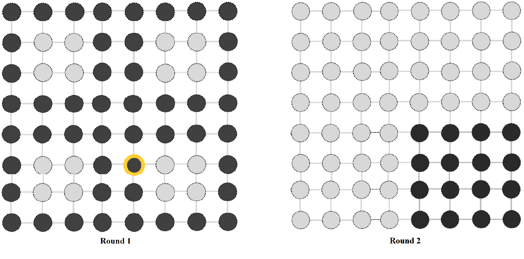
Figure 1: Two dimensional grid of size $8\times 8$. Suppose there are two rounds. In round $1$ the algorithm queries all the black points and selects the minimum among all these points (illustrated with a yellow boundary). In round 2, it queries the entire sub-square in which the minimum from the first round was found.

Algorithm 1: Local search in constant rounds

1. Initialize the current cube to $C_{0}$.

2. In each round $i\in\{1,\ldots,k-1\}$:

   • Divide the current cube $C_{i-1}$ into a set of mutually exclusive sub-cubes $C_{i}^{1},\ldots,C_{i}^{n_{i}}$ of side length $\ell_{i}$ that cover $C_{i-1}$.

   • Query all the points on the boundary of sub-cubes $C_{i}^{1},\ldots,C_{i}^{n_{i}}$. Let $\mathbf{x}^{*}_{i}$ be the point with minimal value among them.

   • Set $C_{i}=C_{i}^{j}$, where $C_{i}^{j}$ is the sub-cube that $\mathbf{x}^{*}_{i}$ belongs to.

3. In round $k$, query all the points in the current cube $C_{k-1}$ and find the solution point.

To argue that the algorithm finds a local minimum, note that in each round $i\leq k-1$, the steepest descent starting from $\mathbf{x}^{*}_{i}$ will never leave the sub-cube $C_{i}$, since if it did it would have to exit $C_{i}$ through a point of even smaller value than $\mathbf{x}_{i}^{*}$, which contradicts the definition of $\mathbf{x}_{i}^{*}$. Thus there must exist a local optimum within $C_{i}$.

Now we calculate the number of queries in each round. In round $i\in\{1,\ldots,k-1\}$, the number of points on the boundary of all sub-cubes $S_{1},\ldots,S_{n_{i}}$ is ${\ell_{i}}^{d-1}\cdot 2d\cdot\left({\ell_{i-1}}/{\ell_{i}}\right)^{d}$, which is equal to $2d\cdot n^{\frac{d^{k+1}-d^{k}}{d^{k}-1}}\,.$ The number of queries in round $k$ is $(\ell_{k-1})^{d}=n^{\frac{d^{k+1}-d^{k}}{d^{k}-1}}$. Since $k$ and $d$ are constants, the algorithm makes $O\left(n^{\frac{d^{k+1}-d^{k}}{d^{k}-1}}\right)$ queries in total as required. ∎

4.1.2 Lower bound overview for local search in constant rounds.

To show lower bounds, we apply Yao’s minimax theorem [Yao77]: first we provide a hard distribution of inputs, then show that no deterministic algorithm could achieve accuracy larger than some constant on this distribution.

The hard distribution will be given by a staircase construction [Vav93, HPV89]. A staircase will be a random path with the property that the unique local optimum is hidden at the end of the path. We present a sketch here; see Appendix B for the complete calculations.

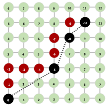
(a) Staircase in 2D for 3 rounds.

(b) Stylized staircase in 2D.

Figure 2: Figure (a) shows a two dimensional staircase for $k=3$ rounds. The number of black points is equal to $k+1$. The black points are connected by “folded segments” shown in red. The idea is that in each round, the algorithm will learn at most one more folded segment. Figure (b) shows in a stylized way the process of selecting the next part of the staircase given that the first folded segment was determined. The folded segments are displayed here as straight lines for simplicity.

An example of a staircase is given in Figure 2; it consists of the black and red vertices. The bottom left black vertex is the starting point of the staircase and the value of the function there is set to zero. Then the value decreases by one with each step along the path, like going down the stairs. The value of the function at any point outside the staircase is equal to the distance to the entrance of the staircase.

Intuitively, the algorithm cannot find much useful structural information of the input and thus has no advantage over a path following algorithm. The staircase construction can be embedded in two different tasks: finding a local minimum of a function [Ald83, Aar06, SY09, Zha09, HY17] and computing a Brouwer fixed-point [CT07, HPV89].

The most challenging part is rigorously proving that such intuition is correct. Our main technical innovation is a new technique to incorporate the round limit into the randomized lower bounds, as we were not able to obtain a lower bound for rounds using the methods previously mentioned. This could also serve as a simpler alternative method of the classical relational adversarial method[Aar06] in the fully adaptive setting.

Staircase definition.

We define a staircase as an array of connecting grid points $(\mathbf{x}_{0},\mathbf{x}_{1},\ldots,\mathbf{x}_{t})$, for $0\leq t\leq k$. A uniquely determined path called folded segment is used to link every two consecutive points $(\mathbf{x}_{i},\mathbf{x}_{i+1})$. The start point $\mathbf{x}_{0}$ is fixed at corner $\mathbf{1}$, and the remaining connecting points are chosen randomly in a smaller and smaller cube region with previous connecting points as corner. For $k$ round algorithms, we choose a distribution of staircases of “length” $k$, where the length is defined as the number of connecting points in the staircase minus $1$.

Good staircases.

We say that a length $t$ staircase is “good” with respect to a deterministic algorithm $\mathcal{A}$ if for each $1\leq i<t$, any point in the suffix of the staircase (i.e. after connecting point $\mathbf{x}_{i}$ ) is not queried in rounds $1,\ldots,i$, when $\mathcal{A}$ runs on the input generated by this staircase.

The input functions generated by good staircases are like adversarial inputs: $\mathcal{A}$ could only (roughly) learn the location of the next connecting point $\mathbf{x}_{i}$ in each round $i$, and still know little about the staircase from $\mathbf{x}_{i}$ onwards.

We show that if ${9}/{10}$ of all possible length $k$ staircases are good, then the algorithm will make a mistake with probability at least ${7}/{40}$ (Lemma 12). We ensure that each possible staircase is chosen with the same probability; their total number is easy to estimate.

Thus the main technical part of our proof is counting the number of good staircases.

Counting good staircases.

The next properties about the prefix of good staircases are proved in Lemma 11:

P1:

If $s$ is a good staircase, then any “prefix” $s^{\prime}$ of $s$ is also a good staircase.

P2:

Let $s_{1},s_{2}$ be two good staircases with respect to algorithm $\mathcal{A}$. If the first $i+1$ connecting points of the staircases are same, then $\mathcal{A}$ will submit the same queries in rounds $1,\ldots,i+1$ when given as input the functions generated by $s_{1}$ and $s_{2}$, respectively.

We first fix a good staircase $s^{(i-1)}$ of length $i-1$ and consider two good staircases $s_{1},s_{2}$ of length $i$ that have $s^{(i-1)}$ as prefix. By P2, the algorithm $\mathcal{A}$ will make the same queries in rounds $1,\ldots,i+1$ when running on the inputs generated by $s_{1}$ and $s_{2}$, respectively. This enables estimating the total number of good length $i+1$ staircase with $s^{(i-1)}$ as prefix.

By summing over all good staircases of length $i-1$, we get a recursive equation between the number of good staircases of length $i-1$, $i$, and $i+1$. This will be used to show that most staircases of length $k$ are good.

4.2 Local Search in Polynomial Rounds

When the number of rounds $k$ is polynomial in $n$, that is $k=n^{\alpha}$ for some constant $\alpha>0$, the algorithm that yields the upper bound in Theorem 1 is no longer efficient.

We design a different algorithm for this regime and also show an almost matching lower bound. With polynomial rounds we can focus on $d\geq 3$. [SY09] proved a lower bound of $\widetilde{\Omega}(n)$ for fully adaptive algorithm in 2D and the divide-and-conquer algorithm by [LTT93] achieves this bound with only $O(\log(n))$ rounds.

Theorem 2.

(Local search, polynomial rounds) Let $k=n^{\alpha}$, where $\alpha\in\left(0,\frac{d}{2}\right)$ is a constant. The randomized query complexity of local search in $k$ rounds on the $d$-dimensional grid $[n]^{d}$ is:

• $\Theta\left(n^{(d-1)-\frac{d-2}{d}\alpha}\right)$ when $d\geq 5$;

• $O\left(n^{3-\frac{\alpha}{2}}\right)$ and $\widetilde{\Omega}\left(n^{3-\frac{\alpha}{2}}\right)$ if $d=4$;

• $O\left(n^{2-\frac{\alpha}{3}}\right)$ and $\Omega\left(\max(n^{2-\frac{2\alpha}{3}},n^{\frac{3}{2}})\right)$ if $d=3$.

When $\alpha\rightarrow 0$, the bound approaches $\Theta(n^{d-1})$, i.e., the bound of constant and logarithmic rounds algorithm. When $\alpha\rightarrow({d}/{2})$, the upper bound is close to $\Theta(n^{\frac{d}{2}})$, i.e., the fully adaptive algorithm. Thus, our result fills the gaps between constant (or logarithmic) rounds algorithms and fully adaptive algorithms, except for a small gap when $d\in\{3,4\}$.

4.2.1 Upper bound overview for local search in polynomial rounds.

The constant rounds algorithm is not optimal when polynomial rounds are available for any $d\geq 3$. Our approach is to randomly sample many points in round $1$ and then start searching for the solution from the best point in round $1$. This is similar to the algorithm in [Ald83], except the steepest descent part of Aldous’ algorithm is highly sequential.

To get better parallelism, we design a recursive procedure (“fractal-like steepest descent”) which parallelizes the steepest descent steps at the cost of more queries. We present the high level ideas next; the formal proof can be found in Appendix A.

Sequential procedure.

Let $C(\mathbf{x},s)\coloneqq\{\mathbf{y}\in[n]^{d}:\|\mathbf{y}-\mathbf{x}\|_{\infty}\leq s\}$ be the set of grid points in the $d$-dimensional cube of side length $2\cdot s$, centered at point $\mathbf{x}$. Let $rank(\mathbf{x})$ be the number of points with smaller function value than point $\mathbf{x}$.

Assume we already have a procedure $P$ and a number $s<n$ such that $P(\mathbf{x})$ will either return a point $\mathbf{y}\in C(\mathbf{x},s)$ with $rank(\mathbf{y})\leq rank(\mathbf{x})-s$, or output a correct solution and halt. Suppose in both cases $P(\mathbf{x})$ takes at most $r$ rounds and $Q$ queries in total for any $\mathbf{x}$.

If we want to find a point $\mathbf{x}^{*}$ with $rank(\mathbf{x}^{*})\leq rank(\mathbf{x}_{0})-t\cdot s$ for any given $\mathbf{x}_{0}$ or output a correct solution, the naive approach is to run $P$ sequentially $t$ times, taking

$$\mathbf{y}_{1}=P(\mathbf{x}_{0}),\mathbf{y}_{2}=P(\mathbf{y}_{1}),\ldots,\mathbf{x}^{*}=\mathbf{y}_{t}=P(\mathbf{y}_{t-1}).$$

Since each call of $P$ must wait for the result from the previous call, the naive approach will take $t\cdot r$ rounds and $t\cdot Q$ queries.

Parallel procedure.

We can parallelize the previous procedure $P$ using auxiliary variables that are more expensive in queries, but cheap in rounds. For $i\in[t]$, let $\mathbf{x}_{i}$ be the point with minimum function value on the boundary of cube $C(\mathbf{x}_{i-1},s)$, which can be found in only one round with $O(s^{d-1})$ queries after getting $\mathbf{x}_{i-1}$, i.e., we get the location of $\mathbf{x}_{i-1}$ at the start of round $i$. Next, we take $\mathbf{y}_{i}$ to be $P(\mathbf{x}_{i-1})$ instead of $P(\mathbf{y}_{i-1})$; thus the location of $\mathbf{y}_{i}$ will be available at round $i+r$. To ensure correctness, we will compare the value of point $\mathbf{y}_{i}$ with the value of point $\mathbf{x}_{i}$. If $f(\mathbf{x}_{i})\leq f(\mathbf{y}_{i})$ then

$$rank(\mathbf{x}_{i})\leq rank(\mathbf{y}_{i})\leq rank(\mathbf{x}_{i-1})-s\,.$$ (1)

Otherwise, since $\mathbf{y}_{i}\in C(\mathbf{x}_{i-1},s)$ has smaller value than any point on the boundary of $C(\mathbf{x}_{i-1},s)$, we could use a slightly modified version of the divide-and-conquer algorithm of [LTT93] to find the solution within the sub-cube $C(\mathbf{x},s)$ in $\log n$ rounds and $O(s^{d-1})$ queries, and then halt all running procedures. If $f(\mathbf{x}_{i})\leq f(\mathbf{y}_{i})$ holds for any $i$, applying inequality 1 for $t$ times we will get $rank(\mathbf{x})\leq rank(\mathbf{x}_{t})-t\cdot s$, so we could return $\mathbf{x}^{*}=\mathbf{x}_{t}$ in this case. This parallel approach will take only $t+r$ rounds and $O(t\cdot(Q+s^{d-1}))$ queries.

The base case of procedure $P$ is the steepest descent algorithm. Then, multiple layers of the recursive process as described above are implemented to ensure the round limit is met. The parameters of the algorithm, such as $s$ and $t$ above, are described in Section A.

4.2.2 Lower bound overview for local search in polynomial rounds.

For polynomial rounds, we still use a staircase construction and hide the solution at the end of the staircase. Recall the bottom left vertex will be the starting point of the staircase and the value of the function there is set to zero. Then the value decreases by one with each step along the path. The value of the function at any point outside the staircase is equal to the distance to the entrance of the staircase.

However, the case of polynomial number of rounds is both conceptually and technically more challenging. We explain the main ideas next; the full proof is in Appendix C.

Choice of random walk

Let $\mathcal{Q}_{k}$ denote the total number of queries allowed for an algorithm that runs in $k$ rounds. Let $\mathcal{Q}=\mathcal{Q}_{k}/k$ be the average number of queries in each round. The minimum point among $\mathcal{Q}_{k}/2$ uniformly random queries will be at most $100\cdot n^{d}/\mathcal{Q}_{k}$ steps away from the solution with high probability.

We set the number of points in the staircase to $\Theta(n^{d}/\mathcal{Q}_{k})$. This strikes a balance between two extremes. If the staircase is too long, then an algorithm like steepest descent with warm-start [Ald83], which starts by querying many random points in round $1$, is likely to hit the staircase in a region that is O$(n^{d}/\mathcal{Q}_{k})$ close to the endpoint. If the staircase is too short, then an algorithm such as steepest descent will find the end of the staircase in a few rounds.

Since we choose the staircase via a random walk, there are two factors affect the difficulty of finding the solution: the mixing time and what we call the “local predictability” of the walk.

Figure 3: A 2D illustration for two types of random walk for the lower bound in polynomial rounds. The random walk on the left is more convoluted locally, but also mixes slower; the walk on the right has simpler structure, but mixes faster.

Consider the random walks in Figure 3. The first random walk ( Figure 3, left) randomly moves to one of its neighbor in each step. This random walk has very low local predictability and may be difficult for fully adaptive algorithms to learn. However, it mixes more slowly, which could be exploited by an algorithm with multiple queries per round.

The second random walk (Figure 3, right) moves from $x_{0}$ to a uniform random point $x_{1}$ selected from a cube of side length $\ell$ centered at $x_{0}$ and uses $d$ straight segments to connect these two points. This random walk is more locally predictable, since each straight segment of length $O(\ell)$ could be learned with $O(\log\ell)$ queries via binary search. Thus the walk could be learned efficiently by a fully adaptive algorithm. On the other hand, the random walk mixes faster than the one in the left figure: it takes only $O(\ell)$ points to mix in the cube region of side length $\ell$. Thus, the second random walk is better when there aren’t enough rounds to find each straight segment via binary search.

By controlling the parameter $\ell$, we get a trade-off between the mixing time and the local predictability when the total length of the walk is fixed. We choose $\ell=\Theta(\mathcal{Q}^{1/(d-1)})=n^{1-2\alpha/d}$ for $k=n^{\alpha}$ in our proof, which corresponds to the max possible side length of the cube if using $\mathcal{Q}$ queries to cover its boundary.

Measuring the Progress

Good staircases are a central concept in the proof for constant rounds. Roughly, the algorithm can learn the location of exactly one more connecting point in each round. However, such a requirement is too strong with polynomial rounds.

Instead, we will allow the algorithm to learn more than one connecting points in some rounds, while showing that it learns no more than two connecting points in each round in expectation.

Using amortized analysis, we quantify the maximum possible progress of an algorithm in each round by a constant $\Gamma$, which only depends on the random walk, not the algorithm. Constant $\Gamma$ could be viewed as the difficulty of the random walk, which takes both the mixing time and the local predictability into account.

5 Brouwer

The problem of finding an $\epsilon$-approximate fixed point of a continuous function was defined in Section 3. To quantify the query complexity of this problem, it is useful to consider a discrete version, obtained by discretizing the unit cube $[0,1]^{d}$. The discrete version of Brouwer was shown to be equivalent to the approximate fixed point problem in the continuous setting in [CD05].

Theorem 3.

Let $k\in\mathbb{N}$ be a constant. For any $\epsilon>0$, the query complexity of the $\epsilon$-approximate Brouwer fixed-point problem in the $d$-dimensional unit cube $[0,1]^{d}$ with $k$ rounds is $\Theta\left((1/\epsilon)^{\frac{d^{k+1}-d^{k}}{d^{k}-1}}\right)$, for both deterministic and randomized algorithms.

We consider only constant rounds, since Brouwer can be solved optimally in a logarithmic number of rounds. The algorithm for Brouwer is reminiscent of the constant rounds algorithm for local search.

We divide the space in sub-cubes of side length $\ell_{i}\coloneqq n^{\frac{d^{k}-d^{i}}{d^{k}-1}}$ in round $i$ and then find the one guaranteed to have a solution by checking a boundary condition given in [CD05]. Then a parity argument will show there is always a sub-cube satisfying the boundary condition. In the last round, the algorithm queries all the points in the remaining sub-cube and returns the solution.

The randomized lower bound for Brouwer is obtained by reducing local search instances generated by staircases to discrete fixed-point instances. We can naturally let the staircase within the local search instance to be the long path in discrete fixed-point problem.

Appendix A Algorithm for Local Search in Polynomial Rounds

The algorithm for polynomial number of rounds was described in Section 4.2. Here we present the precise definition and the proof of correctness.

Notation.

Let the number of rounds be $k=n^{\alpha}$, where $\alpha\in(0,{d}/{2})$ is a constant. Given a point $\mathbf{x}$ on the grid, let $rank(\mathbf{x})$ be the number of grid points with smaller value than point $\mathbf{x}$. Let $C(\mathbf{x},s)\coloneqq\{\mathbf{y}\in[n]^{d}:\|\mathbf{y}-\mathbf{x}\|_{\infty}\leq s\}$ be the set of grid points in the $d$-dimensional cube of side length $2\cdot s$, centered at point $\mathbf{x}$.

Define $h:=\bigl{\lfloor}{1}/{\alpha}+({d-2})/{d}\bigr{\rfloor}+1$; $\;\widetilde{k}:={k}/{h}$ and $\;\beta:=(d-1)-(d-2)\cdot\alpha/{d}$. In the following, a point $\mathbf{x}$ is the minimum in a set $S$ if $\mathbf{x}\in S$ and $f(\mathbf{x})\leq f(\mathbf{y})$ for all $\mathbf{y}\in S$.

There are multiple query requests from different procedures in one round. These queries will first be collected together and then submitted at once at the end of each round.

Algorithm 2: Local search in polynomial number of rounds.

Input: Size of the instance $n$, dimension $d$, round limit $k=n^{\alpha}$, value function $f$. These are global parameters accessible from any subroutine. Output: Local minimum $\mathbf{x}^{*}$ in $[n]^{d}$.

1. Set $\beta\leftarrow(d-1)-\alpha\bigl{(}\frac{d-2}{d}\bigr{)}$ ; $h\leftarrow\bigl{\lfloor}\frac{1}{\alpha}+\frac{d-2}{d}\bigr{\rfloor}+1$ ; $\widetilde{k}\leftarrow{k}/{h}$

2. Query $100\cdot h\cdot n^{\beta}$ points chosen u.a.r. in round $1$ and set $\mathbf{x}_{1}$ to the minimum of these

3. Set $s\leftarrow({1}/{h})\cdot{n^{1+\alpha\left({d-2}\right)/{d}}}$

4. Return FLSD$(s,h,\mathbf{x}_{1},2)$

Procedure Fractal-like Steepest Descent (FLSD).

Input: size $s$, depth $D$, grid point $\mathbf{x}$, round $r$. Output: point $\mathbf{x}^{*}\in C(\mathbf{x},s)$ with $rank(\mathbf{x}^{*})\leq rank(\mathbf{x})-s$; if in the process of searching for such a point it finds a local minimum, then it outputs it and halts everything.

1. Set $\mathbf{x}_{0}\leftarrow\mathbf{x}\;;\;step\leftarrow{s}/{\widetilde{k}}\;\;$ // executed in round $r$

2. If $D=1$ then: // make $s$ steps of steepest descent, since $s$ is small enough when $D=1$

   1. For $i=0$ to $s-1$: // executed in rounds $r+i$ to $r+i+1$

      1. Query all the neighbors of $\mathbf{x}_{i}$; let $\mathbf{x}_{i+1}$ be the minimum among them

      2. If $\mathbf{x}_{i}=\mathbf{x}_{i+1}$ then: // thus $\mathbf{x}_{i}$ is a local min

         Output $\mathbf{x}^{*}\leftarrow\mathbf{x}_{i}$ and halt all running FLSD and DACS calls  

   2. Return $\mathbf{x}^{*}\leftarrow\mathbf{x}_{s}\;\;$ // executed in round $r+s$

3. For $i=0$ to $\widetilde{k}-1$: // divide the whole task into $\widetilde{k}$ pieces; executed in rounds $r+i$ to $r+i+1$

   1. $\mathbf{y}_{i+1}\leftarrow$FLSD$(step,D-1,\mathbf{x}_{i},r+i)$ // execute call in parallel with current procedure

   2. Query the boundary of $C(\mathbf{x}_{i},step)$ to find the point $\mathbf{x}_{i+1}$ with minimum value on it // making a “giant step” of size step by cheap substitute $\mathbf{x}_{i}$

4. For $i=0$ to $\widetilde{k}-1$: // check if each giant step does make giant progress by using the feedback from sub-procedures; executed in round $r+i+(D-1)\cdot\widetilde{k}$, after $y_{i+1}$ was received in Step 3.a.

   1. If $f(\mathbf{y}_{i+1})<f(\mathbf{x}_{i+1})$ then: // a solution exists in $C(\mathbf{x}_{i},step)$, call DACS to find it

      1. Set $\mathbf{x}^{*}\leftarrow$ DACS$(C(\mathbf{x}_{i},step))$ // stop and wait for the result of DACS

      2. Output $\mathbf{x}^{*}$ and halt all running FLSD and DACS calls

5. Return $\mathbf{x}^{*}\leftarrow\mathbf{x}_{\widetilde{k}}$ // executed in round $r+D\cdot\widetilde{k}$

Procedure Divide-and-Conquer Search (DACS).

Input: cube $C_{0}$. Output: Local minimum $\mathbf{x}^{*}$ in $C_{0}$.

1. Set $\mathbf{x}^{*}\leftarrow$ Null

2. For $i=1$ to $\lceil\log_{2}n\rceil$:

   1. If $C_{i-1}$ contains only one point $\widetilde{\mathbf{x}}$ then:

      1. Set $\mathbf{x}^{*}=\widetilde{\mathbf{x}}$ ; break

   2. Partition $C_{i-1}$ into $2^{d}$ disjoint sub-cubes $C_{i}^{1},\ldots,C_{i}^{2^{d}}$, each with side length half that of $C_{i-1}$

   3. Query all the points on the boundary of each sub-cube $C_{i}^{1},\ldots,C_{i}^{2^{d}}$.

   4. Let $\mathbf{x}^{*}_{i}$ be the point with minimum value among all points queried in $C_{i-1}$, including queries made by Algorithm 2 and all FLSD calls // break ties lexicographically

   5. Let $C_{i}\in\{C_{i}^{1},\ldots,C_{i}^{2^{d}}\}$ be the unique sub-cube with $\mathbf{x}^{*}_{i}\in C_{i}$.

3. Return $\mathbf{x}^{*}$

Analysis

We first establish that Algorithm 2 is correct.

Lemma 4.

If the procedure FLSD$(s,D,\mathbf{x},r)$ does return at Step 2.b. or Step 5., it will return within $\widetilde{k}\cdot D$ rounds after the start round $r$; otherwise procedure FLSD$(s,D,\mathbf{x},r)$ will halt within at most $\widetilde{k}\cdot D+\lceil\log n\rceil$ rounds after the start round $r$.

Proof.

We proceed by induction on the depth $D$. The base case is when $D=1$. By the definition of $\widetilde{k}$ and $h$, we have

$$\left(1/{\widetilde{k}}^{h}\right)\cdot n^{1+\frac{d-2}{d}\alpha}<1\,.$$

Also notice that the parameter $s$ will be divided by $\widetilde{k}$ when $D$ decreases by one, so when $D=1$, the current size $s$ will be at most $\widetilde{k}$, i.e., the steepest descent will return in $\widetilde{k}$ rounds. Assume it holds for $1,\ldots,D-1$.

For any $D>1$, all the queries made by the procedure itself need $\widetilde{k}$ rounds and each sub-procedure will take at most $\widetilde{k}\cdot(D-1)$ rounds by the induction hypothesis. Since all the procedures are independent of each other and could be executed in parallel, the total number of rounds needed for this procedure is $\widetilde{k}\cdot D$. The first part of the lemma thus follows by induction.

Finally, recall that the divide-and-conquer procedure DACS takes $\lceil\log n\rceil$ rounds, so the procedure will halt within $\widetilde{k}\cdot D+\lceil\log n\rceil$ rounds. ∎

Lemma 5.

If the procedure FLSD$(s,D,\mathbf{x},r)$ does return a point $\mathbf{x}^{*}$ at Step 2.b. or Step 5., then $\mathbf{x}^{*}$ is in the cube $C(\mathbf{x},s)$ and satisfy the inequality $rank(\mathbf{x}^{*})\leq rank(\mathbf{x})-s$.

Proof of Lemma 5.

We proceed by induction on the depth $D$. The base case is when $D=1$. Then we know that $s\leq\widetilde{k}$ by the same argument in Lemma 4, thus $s$ of steps of steepest descent will ensure that $\mathbf{x}^{*}\in C(\mathbf{x},s)$ and $rank(\mathbf{x}^{*})\leq rank(\mathbf{x})-s$. Assume it holds for $1,\ldots,D-1$ and show for $D$.

For any $D>1$, by Step 4.a. we have $rank(\mathbf{x}_{i})\leq rank(\mathbf{y}_{i})$ for any $1\leq i\leq\widetilde{k}$; by the induction hypothesis, we have $rank(\mathbf{y}_{i})\leq rank(\mathbf{x}_{i-1})-step$ for any $1\leq i\leq\widetilde{k}$. Combining them we get $rank(\mathbf{x}_{i})\leq rank(\mathbf{x}_{i-1})-step$ for any $1\leq i\leq\widetilde{k}$. Thus

$$rank(\mathbf{x}^{*})=rank(\mathbf{x}_{\widetilde{k}})\leq rank(\mathbf{x}_{0})-\widetilde{k}\cdot step=rank(\mathbf{x})-s.$$

Also notice that the $L_{\infty}$ distance from $\mathbf{x}^{*}$ to $\mathbf{x}$ is at most $\widetilde{k}*step=s$, i.e., $\mathbf{x}^{*}\in C(\mathbf{x},s)$. This concludes the proof of the lemma for any depth $D$. ∎

Lemma 6.

The point $\mathbf{x}^{*}$ returned at Step 4.(a.)i is a a local minimum.

Proof.

We use notation $\mathcal{D}.\mathbf{x}$ to denote the variable $\mathbf{x}$ in the procedure DACS and $\mathcal{F}.\mathbf{x}$ to denote the variable $\mathbf{x}$ in the procedure FLSD which calls the procedure DACS.

By Step 4.a., we have $f(\mathcal{F}.\mathbf{y}_{i+1})<f(\mathcal{F}.\mathbf{x}_{i+1})$. Then for each $\mathcal{D}.\mathbf{x}^{*}_{i},i$, we have $f(\mathcal{D}.\mathbf{x}^{*}_{i})\leq f(\mathcal{F}.\mathbf{y}_{i+1})<f(\mathcal{F}.\mathbf{x}_{i+1})$ by its definition. Therefore the steepest descent from $\mathcal{D}.\mathbf{x}^{*}_{i}$ will never leave the cube $\mathcal{D}.C_{i}$, especially the cube $\mathcal{D}.C_{0}$. Let $\widetilde{C}$ be the cube that consists only of the point $\mathcal{D}.\widetilde{\mathbf{x}}$ in the DACS procedure. The steepest descent from $\mathcal{D}.\mathbf{x}^{*}=\mathcal{D}.\widetilde{\mathbf{x}}$ doesn’t leave the cube $\widetilde{C}$, which means that $\mathcal{D}.\mathbf{x}^{*}$ is a local optimum. ∎

Lemma 7.

Algorithm 2 outputs the correct answer with probability at least ${9}/{10}$.

Proof.

The point $\mathbf{x}^{*}$ output at Step 2.(a.)ii is always a local optimum. By Lemma 6, the point $\mathbf{x}^{*}$ output at Step 4.(a.)ii is also a local optimum. Thus we only need to argue that the Algorithm 2 will output the solution and halt with probability at least ${9}/{10}$. Notice that

$$\frac{n^{d}}{100h\cdot n^{\beta}}=\frac{1}{100h}n^{1+\frac{d-2}{d}\alpha}.$$

Thus after the first round, with probability at least ${9}/{10}$, we have

$$rank(\mathbf{x}_{1})\leq\frac{1}{2h}n^{1+\frac{d-2}{d}\alpha}\,.$$ (2)

If inequality (2) holds, then the procedure FLSD$({1}/{h}\cdot{n^{1+\frac{d-2}{d}\alpha}},h,\mathbf{x}_{1},2)$ should halt within a number of rounds of at most

$$T=\widetilde{k}\cdot\left((h-1)+\frac{2}{3}\right)+\lceil\log n\rceil<\widetilde{k}\cdot h=k.$$

Otherwise, let $t=\lfloor{2\widetilde{k}}/{3}\rfloor$. By Lemma 4 we know that $y_{t}$ is already available from Step 3.a. by round $T$. Then by Lemma 5, we have

$$rank(\mathbf{y}_{t})<\left(\frac{1}{2}-\frac{2}{3}\right)\cdot\left(\frac{1}{h}n^{1+\frac{d-2}{d}\alpha}\right)<0,$$

which is impossible. Thus, the call FLSD$(1/h\cdot{n^{1+\frac{d-2}{d}\alpha}},h,\mathbf{x}_{1},2)$ must halt within $T$ rounds in this case, which completes the argument. ∎

Now consider the total number of queries made by Algorithm 2.

Lemma 8.

A call of procedure FLSD$(s,D,\mathbf{x},r)$ will make $O(\lceil s/\widetilde{k}\rceil^{d-1}\cdot\widetilde{k})$ number of queries, including the queries made by its sub-procedure.

Proof.

We proceed by induction on the depth $D$. The base case is when $D=1$. In this case, the procedure FLSD performs $s$ steps of steepest descent, where $s\leq\widetilde{k}$. Thus it will make $s\cdot 2d=O(\widetilde{k})$ queries.

For any depth $D>1$,

• the number of queries made by Step 3.b. is at most

  $$2d\cdot(2\lceil s/\widetilde{k}\rceil+1)^{d-1}\cdot\widetilde{k}=O(\lceil s/\widetilde{k}\rceil^{d-1}\cdot\widetilde{k});$$

• the number of queries made by all sub-procedures is bounded as follows by the induction hypothesis

  $$\widetilde{k}\cdot O\left(\lceil{s}/{{\widetilde{k}}^{2}}\rceil^{d-1}\cdot\widetilde{k}\right)=O(\lceil s/\widetilde{k}\rceil^{d-1}\cdot\widetilde{k});$$

• the number of queries made by DACS is at most

  $$(2\lceil s/\widetilde{k}\rceil+1)^{d-1}\cdot 2d\cdot 2=O(\lceil s/\widetilde{k}\rceil^{d-1}).$$

Thus the total number of queries is $O(\lceil s/\widetilde{k}\rceil^{d-1}\cdot\widetilde{k})$, which concludes the proof for all $D$. ∎

Proof of Upper Bound of Theorem 2.

The correctness of Algorithm 2 is established by Lemma 7. By Lemma 8, the total number of queries issued by Algorithm 2 is

$$100h\cdot n^{(d-1)-\frac{d-2}{d}\alpha}+O((n^{1-\frac{2\alpha}{d}})^{d-1}\cdot({n^{\alpha}}/{h}))=O(n^{(d-1)-\frac{d-2}{d}\alpha})\,.$$

This concludes the proof of the upper bound part in Theorem 2. ∎

Appendix B Randomized Lower Bound for Local Search in Constant Rounds

In this section we show the lower bound for local search in constant number of rounds. We start with a few definitions.

Notation and Definitions

Recall that $\ell_{i}=n^{\frac{d^{k}-d^{i}}{d^{k}-1}},0\leq i<k$. Let $m\coloneqq\sum_{0\leq i<k}\ell_{i}\leq 2n$. We now consider the grid of side length $m$ in this subsection for technical convenience.

For a point $\mathbf{x}=(x_{1},\ldots,x_{d})$, let $W_{i}(\mathbf{x})$ be the grid points that are in the cube region of size $(\ell_{i})^{d}$ with corner point $\mathbf{x}$:

$$W_{i}(\mathbf{x})=\{\mathbf{y}=(y_{1},\ldots,y_{d})\in[m]^{d}:x_{j}\leq y_{j}<x_{j}+\ell_{i},\forall j\in[d]\}\,.$$

Next we define a basic structure called folded-segment. Intuitively, the folded-segment connecting two points $\mathbf{x},\mathbf{y}$ is the following path of points: Starting at point $\mathbf{x}$, we initially change the first coordinate of $\mathbf{x}$ towards the first coordinate of $\mathbf{y}$. Then we change the second coordinate, the third coordinate, and so on, until finally reaching the point $\mathbf{y}$. The formal definition is as follows.

Definition 9 (folded-segment).

For any two points $\mathbf{x},\mathbf{y}\in[m]^{d}$ , the folded-segment $FS(\mathbf{x},\mathbf{y})$ is a set of points connecting $\mathbf{x}$ and $\mathbf{y}$, defined as follows.

Let $\mathbf{x}=(x_{1},\ldots,x_{d}),\mathbf{y}=(y_{1},\ldots,y_{d})$. For any $1\leq i\leq d$, define point set

$$E_{i}(\mathbf{x},\mathbf{y})\coloneqq\{\mathbf{z}=(y_{1},\ldots,y_{i-1},z_{i},x_{i+1},\ldots,x_{d})\in[m]^{d}:\min(x_{i},y_{i})\leq z_{i}\leq\max(x_{i},y_{i})\}.$$

Then define

$$FS(\mathbf{x},\mathbf{y})=(\bigcup_{i\in[d]}E_{i}(\mathbf{x},\mathbf{y}))\backslash\{\mathbf{x}\}$$

Staircase Structure

A staircase $s^{(i)}(\mathbf{x}_{0},\mathbf{x}_{1},\ldots,\mathbf{x}_{i})$ of length $i$, where $0\leq i\leq k$, consists of a path of points defined by an array of $i+1$ “connecting” points $\mathbf{x}_{0},\mathbf{x}_{1},\ldots,\mathbf{x}_{i}\in[m]^{d}$. We call $\mathbf{x}_{0}$ as the start point and $\mathbf{x}_{i}$ as the end point. For each $0\leq j<i$, the pair of consecutive connecting points $(\mathbf{x}_{j},\mathbf{x}_{j+1})$ is connected by a folded-segment $FS(\mathbf{x}_{j},\mathbf{x}_{j+1})$. We denote the $j$-th ($0\leq j\leq i$) connecting point of $s^{(i)}$ as $\mathbf{x}_{j}$, and the $j$-th ($1\leq j\leq i$) folded-segment of $s^{(i)}$ as $FS(\mathbf{x}_{j-1},\mathbf{x}_{j})$.

The probability distribution for staircases of length $i$, where $0\leq i\leq k$, is as follows. The start point $\mathbf{x}_{0}$ is always set to be the corner point $\mathbf{1}$; points $\mathbf{x}_{1},\mathbf{x}_{2},\ldots,\mathbf{x}_{i}$ are picked in turn: the point $\mathbf{x}_{j}$ is chosen uniformly random from the sub-cube $W_{j-1}(\mathbf{x}_{j-1})$. Two staircases are different if they have different set of connecting points, even if the paths defined by the two sets of connecting points are the same. Thus, $L^{(i)}\coloneqq\Pi_{j=0}^{i-1}\,{\ell_{j}}^{d}$ is the number of all possible length $i$ staircases, and each staircase will be selected with the same probability ${1}/{L^{(i)}}$.

A staircase $s$ of length $i$ grows from a staircase $s^{\prime}$ of length $(i-1)$ if the first $i-1$ folded-segment of $s$ and $s^{\prime}$ are same. A prefix of staircase $s$ is any staircase formed by a prefix of the connecting points sequence of $s$. To simplify the analysis, we assume the algorithm is given the location of $\mathbf{x}_{i}$ after round $i$, except for the round $k$; this only strengthens the lower bound.

Value Function

After fixing a staircase $s$, we can define the value function $f^{s}$ corresponding to $s$. Within the staircase, the value of the point is minus the distance to $\mathbf{x}_{0}$ by following the staircase backward, except the end point $\mathbf{x}_{i}$ of the staircase. The value of any point outside is the $L_{1}$ distance to $\mathbf{x}_{0}$. The value of the end point $\mathbf{x}_{i}$ is set as minus the distance to the point $\mathbf{x}_{0}$ by following the staircase backward with probability $1/2$, and the $L_{1}$ distance to $\mathbf{x}_{0}$ with probability $1/2$. Thus the end point of the staircase must be queried, otherwise the algorithm will incorrectly guess the location of the unique solution point with probability at least $1/2$.

This value function makes sure that for any two different staircases $s_{1}$ and $s_{2}$, the functions $f^{s_{1}}$ and $f^{s_{2}}$ have the same value on the common prefix and on any point outside of both $s_{1}$ and $s_{2}$. Also notice that $f^{s}$ is deterministic on every point except the end point $\mathbf{x}_{i}$ of staircase $s$.

Good Staircases

Next we introduce the concept of good staircases, on which the algorithm could only learn one more connecting point in each round.

Definition 10 (good staircase).

A staircase $s^{(i)}(\mathbf{x}_{0},\ldots,\mathbf{x}_{i})$ of length $i$ is good with respect to a deterministic algorithm $\mathcal{A}$ that runs in $k$-rounds, if the following condition is met:

• when $\mathcal{A}$ is running on the value function $f^{s^{(i)}}$, for any $0<j<i$, any point $\mathbf{x}\in FS(\mathbf{x}_{j},\mathbf{x}_{j+1})$ is not queried by algorithm $\mathcal{A}$ in rounds $1,\ldots,j$.

We use good staircase to indicate the good staircase with respect to a fixed deterministic algorithm $\mathcal{A}$ for brevity. Good staircases have the following properties.

Lemma 11.

1. If $s$ is a good staircase, then any prefix $s^{\prime}$ of $s$ is also a good staircase.

2. Let $s_{1},s_{2}$ be any two good staircases. If the first $i+1$ connecting points of the staircases are the same, then $\mathcal{A}$ will receive the same replies in rounds $1,\ldots,i$ and issue the same queries in rounds $1,\ldots,i+1$ while running on both $f^{s_{1}}$ and $f^{s_{2}}$.

Proof.

We first prove part $2$. By the definition of good staircase, in round $1,\ldots,i$, algorithm $\mathcal{A}$ will not query any point on $s_{1}$ or $s_{2}$ that is after the first $i+1$ connecting points, where $f^{s_{1}}$ and $f^{s_{2}}$ may have different value. Since $\mathcal{A}$ is deterministic, by induction from round $1$, we get that $\mathcal{A}$ will issue the same queries and receive the same replies in rounds $1,\ldots,i$. The queries in round $i+1$ are also same because they only depend on the replies in round $1,\ldots,i$. The proof of part $1$ is similar by taking $s_{1}=s$ and $s_{2}=s^{\prime}$. ∎

If most of the possible staircases are good staircases, then $\mathcal{A}$ will fail on a constant fraction of the inputs generated by length $k$ staircases.

Lemma 12.

If the algorithm $\mathcal{A}$ issues at most $\mathcal{Q}_{k}=1/10\cdot n^{\frac{d^{k+1}-d^{k}}{d^{k}-1}}$ queries in each round, and $9/10$ of all possible length $k$ staircases are good , then $\mathcal{A}$ will fail to get the correct solution with probability at least $7/40$.

Proof.

If $s^{(k)}(\mathbf{x}_{0},\ldots,\mathbf{x}_{k-1},\mathbf{x}_{k})$ is good, then $\mathcal{A}$ could not distinguish it from another good staircase $s^{\prime}(\mathbf{x}_{0},\ldots,\mathbf{x}_{k-1},\mathbf{x}_{k}^{\prime})$ with same first $k$ connecting points before the last round by Lemma 11.

Recall that before the last round, the algorithm is given the value of $\mathbf{x}_{k-1}$. Let $z_{s^{(k-1)}}$ be the fraction of length $k$ good staircases among all length $k$ staircases growing from the length $(k-1)$ staircase $s^{(k-1)}$. Then define the random variable $Z$ such that $Z=z_{s^{(k-1)}}$ if the length $(k-1)$ staircase $s^{(k-1)}$ is chosen. Since each length $(k-1)$ staircase is selected with the same probability, the expectation of $Z$ is $9/10$.

Thus by Markov inequality on $(1-Z)$, a half of all the length $(k-1)$ staircases $s^{(k-1)}$ satisfy $z_{s^{(k-1)}}\geq 8/10$. We say a length $(k-1)$ staircase $s^{(k-1)}$ is nice if $z_{s^{(k-1)}}\geq 8/10$.

Recall there are $\left(\ell_{k-1}\right)^{d}=n^{\frac{d^{k+1}-d^{k}}{d^{k}-1}}$ of length $k$ staircases growing from a length $(k-1)$ staircase.

However, the algorithm can only query $1/10\cdot n^{\frac{d^{k+1}-d^{k}}{d^{k}-1}}$ points in the last round. Thus if $s^{(k)}$ is a good staircase growing from a length $k-1$ nice staircase $s^{(k-1)}$, then $\mathcal{A}$ will not query the endpoint $\mathbf{x}_{k}$ of $s^{(k)}$ with probability at least $7/8$. We define the following events:

• Fail = {$\mathcal{A}$ makes mistake}

• Hit = { $\mathcal{A}$ never queries the end point $\mathbf{x}_{k}$ during the execution}

• Nice = {the length $k-1$ prefix $s^{(k-1)}$ of $s^{(k)}$ is nice}

• Good = {the whole length $k$ staircase $s^{(k)}$ is good}.

Thus $\mathcal{A}$ will make a mistake with probability at least

$$\Pr[\mbox{Fail}] \geq\frac{1}{2}\cdot\Pr[\mbox{Hit}]\geq\frac{1}{2}\cdot\Pr[\mbox{Hit}\,|\,\mbox{Nice}\land\mbox{Good}]\cdot\Pr[\mbox{Nice}\land\mbox{Good}]$$

$$\geq\frac{1}{2}\cdot\frac{7}{8}\cdot\Pr[\mbox{Good}\,|\,\mbox{Nice}]\cdot\Pr[\mbox{Nice}]\geq\frac{1}{2}\cdot\frac{7}{8}\cdot\frac{8}{10}\cdot\frac{1}{2}=\frac{7}{40}\,,$$

where the probability is taken on the staircase $s^{(k)}$ and the value of $\mathbf{x}_{k}$. ∎

Counting the number of good staircases

Counting the number of good staircases is the major technical challenge in the proof. The concept of probability score function is useful.

Definition 13 (probability score function).

For a fixed deterministic algorithm $\mathcal{A}$, let $Q_{\mathcal{A}}$ be the set of points queried by $\mathcal{A}$ during its execution. Given a point $\mathbf{x}\in[m]^{d}$ , for any $0\leq i<k$, define the set of points

$$W_{i}(\mathbf{x},Q_{\mathcal{A}})\coloneqq\{\mathbf{y}\in W_{i}(\mathbf{x}):FS(\mathbf{x},\mathbf{y})\cap Q_{\mathcal{A}}=\emptyset\}.$$

The probability score function for the point $\mathbf{x}$ is $SC_{i}(\mathbf{x},Q_{\mathcal{A}})\coloneqq\frac{\left|W_{i}(\mathbf{x},Q_{\mathcal{A}})\right|}{{\ell_{i}}^{d}}$.

The probability score function for a good staircases $s^{(i)}(\mathbf{x}_{0},\ldots,\mathbf{x}_{i})$ of length $i,0\leq i<k$ is defined as $SC(s^{(i)})\coloneqq SC_{i}(\mathbf{x}_{i},Q_{\mathcal{A}})$, where $Q_{\mathcal{A}}$ is the set of points that have been queried by $\mathcal{A}$ after the round $i$, if $\mathcal{A}$ is executed on value function $f^{s^{(i)}}$.

Let $\mathbf{x}\in[m]^{d}$, $\mathbf{y}\in Q_{\mathcal{A}}$. Let $B_{i}(\mathbf{x},\mathbf{y})\coloneqq\{\mathbf{z}\in W_{i}(\mathbf{x}):\mathbf{y}\in FS(\mathbf{x},\mathbf{z})\}.$ Thus $\left|B_{i}(\mathbf{x},\mathbf{y})\right|$ is the number of folded-segments $FS(\mathbf{x},\mathbf{z}),\mathbf{z}\in W_{i}(\mathbf{x})$ that are intersected by a point $\mathbf{y}\in Q_{\mathcal{A}}$. We then define the cost incurred by a point $\mathbf{y}\in Q_{\mathcal{A}}$ on the probability score function of a point $\mathbf{x}$ for any $0\leq i<k$ as

$$cost_{i}(\mathbf{x},\mathbf{y})\coloneqq\frac{\left|B_{i}(\mathbf{x},\mathbf{y})\right|}{{\ell_{i}}^{d}}.$$

The merit of our random staircase structure is that any single queried point will not hit too much of staircases. This property is quantitatively characterized by the following lemma via the cost.

Lemma 14.

The total cost incurred by one point $\mathbf{y}\in Q_{\mathcal{A}}$ for all $\mathbf{x}\in[m]^{d}$, i.e., $\sum_{\mathbf{x}}{\left|B_{i}(\mathbf{x},\mathbf{y})\right|}/({\ell_{i}}^{d})$ is at most $d\cdot{\ell_{i}}$.

Proof.

If $\mathbf{y}\notin W_{i}(\mathbf{x})$, we simply have $cost_{i}(\mathbf{x},\mathbf{y})=0$. Therefore we only need to estimate $cost_{i}(\mathbf{x},\mathbf{y})$ or equivalently, $\left|B_{i}(\mathbf{x},\mathbf{y})\right|$ for pairs $\mathbf{x},\mathbf{y}$ such that $\mathbf{y}\in W_{i}(\mathbf{x})$.

For two points $\mathbf{x}=(x_{1},\ldots,x_{d}),\mathbf{y}=(y_{1},\ldots,y_{d})$, denote $t(\mathbf{x},\mathbf{y})\in[d]$ to be the smallest index such that for any $j$ satisfying $t(\mathbf{x},\mathbf{y})<j\leq d$, there is $x_{j}=y_{j}$. Then, by the definition of folded-segments, we have

$$B_{i}(\mathbf{x},\mathbf{y})=\{(y_{1},\ldots,y_{t(\mathbf{x},\mathbf{y})-1},z_{t(\mathbf{x},\mathbf{y})},z_{t(\mathbf{x},\mathbf{y})+1},\ldots,z_{d})\in W_{i}(\mathbf{x}):z_{t(\mathbf{x},\mathbf{y})}\geq y_{t(\mathbf{x},\mathbf{y})}\}.$$

Therefore, we have $\left|B_{i}(\mathbf{x},\mathbf{y})\right|\leq{\ell_{i}}^{d-t(\mathbf{x},\mathbf{y})+1}$.

Finally, for a point $\mathbf{y}$, the number of points $\mathbf{x}$ such that $\mathbf{y}\in W_{i}(\mathbf{x})$ and $t(x,y)=j$ is at most ${\ell_{i}}^{j}$. Therefore, we have

$$\sum_{\mathbf{x}\in[m]^{d}}\frac{\left|B_{i}(\mathbf{x},\mathbf{y})\right|}{{\ell_{i}}^{d}} =\sum_{j\in[d]}\sum_{\mathbf{x}\in[m]^{d}}\frac{\left|B_{i}(\mathbf{x},\mathbf{y})\right|}{{\ell_{i}}^{d}}\cdot\mathbf{1}[t(\mathbf{x},\mathbf{y})=j]$$ (3)

$$\leq\sum_{j\in[d]}\frac{{\ell_{i}}^{j}\cdot{\ell_{i}}^{d-j+1}}{{\ell_{i}}^{d}}$$ (4)

$$=d\cdot{\ell_{i}}$$ (5)

∎

We can now count the number of length $k$ good staircases with the two-stage analysis, which is formally summarized in below.

Lemma 15.

If the number of queries issued by algorithm $\mathcal{A}$ is at most

$$\mathcal{Q}_{k}=1/{(10d\cdot k})\cdot n^{\frac{d^{k+1}-d^{k}}{d^{k}-1}},$$

then $9/10$ of all possible length $k$ staircases are good with respect to $\mathcal{A}$.

Proof.

For $0\leq i\leq k$, denote $G^{(i)}$ as the set of all good staircases of length $i$. Then $|G^{(i)}|$ is the number of all length $i$ good staircases, and $R^{(i)}\coloneqq|G^{(i)}|/L^{(i)}$ is the fraction of length $i$ good staircases. In particular, $L^{(0)}=|G^{(0)}|=R^{(0)}=1$.

Let’s first fix a length $i\;(0\leq i<k-1)$ good staircase $s^{(i)}\in G^{(i)}$, and denote the set of all good staircases growing from $s^{(i)}$ as $G(s^{(i)})$. Now consider the sum of the probability score function for every staircase in $G(s^{(i)})$. By Lemma 11, algorithm $\mathcal{A}$ will make the same queries in rounds $1,\ldots,i+1$ when running on any instance $f^{s^{(i+1)}}$ generated by staircase $s^{(i+1)}$ in $G(s^{(i)})$. Thus, we can use Lemma 14 and the union bound to upper bound the total cost to the sum of their probability score function:

$$\sum_{s^{(i+1)}\in G(s^{(i)})}SC(s^{(i+1)}) \geq{\ell_{i}}^{d}\cdot SC(s^{(i)})-\mathcal{Q}_{k}\cdot d\ell_{i+1}\geq{\ell_{i}}^{d}\cdot\left(SC(s^{(i)})-\frac{1}{10k}\right)$$ (6)

The second inequality comes from the fact that $\mathcal{Q}_{k}\cdot\ell_{i+1}=\frac{{\ell_{i}}^{d}}{d\cdot(10k)}\,.$

Next, let’s consider the number of all length $i+2$ good staircases.

$$|G^{(i+2)}| =\sum_{s^{(i+1)}\in G^{(i+1)}}SC(s^{(i+1)})\cdot{\ell_{i+1}}^{d}$$ (7)

$$=\sum_{s^{(i)}\in G^{(i)}}\left(\sum_{s^{(i+1)}\in G(s^{(i)})}SC(s^{(i+1)})\cdot{\ell_{i+1}}^{d}\right)$$ (8)

$$\geq({\ell_{i+1}}^{d}\cdot{\ell_{i}}^{d})\cdot\sum_{s^{(i)}\in G^{(i)}}\left(SC(s^{(i)})-\frac{1}{10k}\right)$$ (9)

$$={\ell_{i+1}}^{d}\cdot\left(|G^{(i+1)}|-{\ell_{i}}^{d}\cdot\frac{|G^{(i)}|}{10k}\right)$$ (10)

Equality (7) and equality (10) are from the definition of probability score function. Inequality (9) is from inequality (6). Dividing each side of (10) by $L^{(i+2)}$, we get

$$R^{(i+2)}\geq R^{(i+1)}-\frac{R^{(i)}}{10k}\geq R^{(i+1)}-\frac{1}{10k}\,.$$ (11)

We know that $R^{(1)}=1$ by definition, so $R^{(k)}\geq 9/10$ as required. ∎

The correctness of the lower bound statement in Theorem 1 follows from Lemma 12 and Lemma 15.

Appendix C Randomized Lower Bound for Local Search in Polynomial Rounds

In this section we show the lower bound for local search in polynomial number of rounds.

C.1 Notation and Definitions

Recall the number of rounds is $k=n^{\alpha}$, where $\alpha\in(0,d/2)$. Define $\ell=n^{1-(2/d)\cdot\alpha}$ and $m=n/\ell$, where the definition of $m$ from section B is overridden here.

Define $\mathcal{Q}_{k}$ to be the number of queries allowed for the $k$-round algorithm stated in Theorem 2:

$$\mathcal{Q}_{k}=\left\{\begin{array}[]{ll}c_{d}\cdot n^{(d-1)-\frac{d-2}{d}\alpha}&\textrm{if $d>4$}\\ \frac{c_{4}}{\log n}\cdot n^{3-\frac{1}{2}\alpha}&\textrm{if $d=4$}\\ c_{3}\cdot n^{(d-1)-\frac{2}{3}\alpha}&\textrm{if $d=3$}\end{array}\right.$$ (12)

The value $c_{d}$ above is a constant depending on dimension $d$.

For any point $x\in[n]$ in the 1D grid, define $W^{1}(x)$ as the set of points within $\ell$ steps of going right from $x$, and assuming $1$ is the next point of $n$ by wrapping around. Formally,

$$W^{1}(x)=\{y\in[n]:x<y\leq x+\ell\;\mathrm{or}\;y\leq x+\ell-n\}\,.$$

Similarly, for a point $\mathbf{x}=(x_{1},\ldots,x_{d})$ in the $d$ dimensional grid $[n]^{d}$, let $W(\mathbf{x})$ be the set of grid points that are in the cube region of side length $\ell$ with corner point $\mathbf{x}$, and wrapping around the boundary if exceeding. That is,

$$W(\mathbf{x})=\{\mathbf{y}=(y_{1},\ldots,y_{d})\in[n]^{d}:y_{j}\in W^{1}(x_{j}),\forall j\in[d]\}\,.$$

For any index $i\in[d]$, define

$$W^{-1}_{i}(\mathbf{x})=\{\mathbf{y}\in[n]^{d}:\forall j\leq i,x_{j}\in W^{1}(y_{j});\forall j>i,y_{j}=x_{j}\}$$ (13)

$$W^{b}_{i}(\mathbf{x})=\{\mathbf{y}\in[n]^{d}:\forall j<i,x_{j}\in W^{1}(y_{j});\max\{n-\ell,x_{i}\}<y_{i}\leq n;\forall j>i,y_{j}=x_{j}\}$$ (14)

Let

$$W^{-1}(\mathbf{x})=\bigcup_{i\in[d]}W^{-1}_{i}(\mathbf{x}),W^{b}(\mathbf{x})=\bigcup_{i\in[d]}W^{b}_{i}(\mathbf{x}),W^{r}(\mathbf{x})=W^{-1}(\mathbf{x})\cup W^{b}(\mathbf{x})$$

When calculating the coordinate of points, we always keep wrapping around it into the range $[n]^{d}$ for convenience.

Staircase structure

Let $\mathbf{x}_{0}=\mathbf{1}$ be the corner point. The remaining connecting points $\mathbf{x}_{1},\mathbf{x}_{2},\ldots,\mathbf{x}_{i}$ are selected in turn, where $\mathbf{x}_{j}$ is chosen uniformly from

1. the set $W(\mathbf{x}_{j-1})$, if $(j\;\mathrm{mod}\;m)\neq 0$;

2. the set $[n]^{d}$, otherwise.

We still use the folded-segment as in Definition 9 to link every two consecutive connecting points. The length of a staircase is the number of folded segments in it.

Let $S^{(i)}$ be the set of all possible staircases of length $i$. Let $S^{(i)}(s_{j})$ be the subset of $S^{(i)}$ in which every staircase has staircase $s_{j}$ as prefix. Every possible staircase of length $i$ occurs with the same probability and their total number is $L^{(i)}=\left|S^{(i)}\right|$. Each staircase $s_{i}$ of length $i$ has the same number of length $j$ staircases growing from it, namely, $\left|S^{(i)}(s_{j})\right|=L^{(i)}/L^{(j)}$.

Let $p(\mathbf{x},\mathbf{y},i,t)$ to be the probability that point $\mathbf{y}$ is on the $(i+t-1)$-th folded-segment, conditioned on point $\mathbf{x}$ being the $i$-th connecting point. Similarly, define $q(\mathbf{x},\mathbf{y},i,t)$ as the probability that point $\mathbf{y}$ is the $(i+t)$-th connecting point, conditioned on point $\mathbf{x}$ being the $i$-th connecting point.

Value function

The value function $f^{s}$ for staircase $s$ is determined by the same rule as the constant rounds case in section B.

A point is called a self-intersection point if it lies on multiple folded-segments and we deem it to belong to the folded-segment closest to the solution. Thus, the distance from it to the start point is defined by tracing through all the previous points on the staircase.

Recall an important property of these value functions that if two staircases $s_{1},s_{2}$ share a common length $i$ prefix, then $f^{s_{1}}$ and $f^{s_{2}}$ have same value except for points that are after the $i$-th connecting points of $s_{1}$ or $s_{2}$.

In the rest of this section, we will show that the distribution of value functions generated by all length $K=2k$ staircases is hard for any $k$-rounds deterministic algorithm $\mathcal{A}$ with at most $\mathcal{Q}_{k}$ queries.

C.2 Useful Assumptions

We make several assumptions to simply the proof in this section.

Assumption 1.

Once the algorithm $\mathcal{A}$ queried a point on the $i$-th folded segment $FS(\mathbf{x}_{i-1},\mathbf{x}_{i})$, the location of point $\mathbf{x}_{i}$ and all previous connecting points are provided to the algorithm $\mathcal{A}$.

With this assumption, we can quantify the progress of algorithm $\mathcal{A}$ at a certain round by the number of connecting points it knows, where we say algorithm $\mathcal{A}$ knows or learns the connecting point $\mathbf{x}_{i}$ if $\mathcal{A}$ is already given the location of $\mathbf{x}_{i}$.

Assumption 2.

Algorithm $\mathcal{A}$ learns at least one more connecting point in each round, and it succeeds on a specific input if it knows the location of the end point $\mathbf{x}_{K}$ of the staircase by the end of round $k$.

Notice that assumptions 1 and 2 only make the bound stronger.

If $\mathcal{A}$ learns $t$ more connecting points in one round, we say $\mathcal{A}$ saves $t-1$ rounds, since we expect $\mathcal{A}$ learns exactly one more connecting points in each round by default.

Assumption 3.

Algorithm $\mathcal{A}$ issues the same number of queries in each round, i.e. $\mathcal{Q}\coloneqq\mathcal{Q}_{k}/k$.

Every $k$ rounds algorithm with $\mathcal{Q}_{k}$ queries can be converted to an algorithm in $2k$ rounds with $\mathcal{Q}_{k}/k$ queries in each round. Since we have polynomial number of rounds, a constant factor of 2 won’t matter.

Assumption 4.

Algorithm $\mathcal{A}$ will keep running until it learns the end point of staircase, regardless of the round limit $k$.

A fixed round limit is more technically challenging to deal with. With assumption 4, we could instead argue that any such algorithm $\mathcal{A}$ will run more than $1.1k$ rounds in expectation. Then, by applying Markov inequality, we will show that $\mathcal{A}$ fails to learn the end point of the staircase with probability at least $0.1$ if the round limit $k$ is imposed.

Let $SV(s)$ be the total number of rounds $\mathcal{A}$ saved when $\mathcal{A}$ is running on the input generated by a fixed staircase $s$. By definition, the total number of rounds needed for learning the end point of $s$ is $K-SV(s)$.

With the assumptions and arguments above, the next two subsections are devoted to proving the following lemma, which establishes $\mathcal{Q}_{k}$ as the lower bound.

Lemma 16.

The following inequality holds:

$$\frac{L^{(K)}\cdot K-\sum_{s\in S^{(K)}}SV(s)}{L^{(K)}}\geq 1.1k\;,$$ (15)

where the left hand side is the expected number of rounds needed to learn the end point considering the input distribution generated by length-$K$ staircases.

C.3 Estimate the Savings

Let $r^{s}_{i}$ be the number of the round in which the $i$-th connecting point on staircase $s$ is first known to $\mathcal{A}$ when running on the input $f^{s}$.

Definition 17 (critical point).

The $i$-th connecting point is a critical point of a length $t$ staircase $s$ if $r^{s}_{i}\neq r^{s}_{i+1}$ or $i=t$.

By assumption 1, an equivalent definition is that when the $i$-th connecting point is first learned at round $r^{s}_{i}$, $\mathcal{A}$ has not queried any point that is after the $i$-th connecting point; that is, the $i$-th connecting point is learned by querying a point on the $i$-th folded segment.

Intuitively, each critical point takes one round to learn, while each non-critical points are given for free by assumption 1.

By amortizing the rounds saved for each non-critical points to the next closest critical point, we define $SV(s,i)$ as the number of rounds saved by the $i$-th connecting point of staircase $s$. More formally,

1. $SV(s,i)=i-\max\{j:r^{s}_{j}=r^{s}_{i}-1\}-1$, if $i$-th connecting point is a critical point;

2. $SV(s,i)=0$, otherwise.

By definition, $SV(s)=\sum_{i=1}^{k}SV(s,i)$.

Let $r^{s}_{i,j},j\geq i$ be the number of the round in which the $i$-th connecting point on staircase $s$ is first learned by $\mathcal{A}$, when running on the input generated by the length $j$ prefix of $s$.

Lemma 18.

The following inequality holds: $r^{s}_{i,j}\geq r^{s}_{i}$.

Proof.

Denote the instance generated by the staircase $s$ as $f^{s}$ and the instance generated by the length $j$ prefix of $s$ as $f^{s}_{j}$.

Assume towards a contradiction that $r^{s}_{i,j}<r^{s}_{i}$. Then we prove by induction that the queries made by $\mathcal{A}$ from round $1$ to round $r^{s}_{i,j}$ are the same on inputs $f^{s}$ and $f^{s}_{j}$.

Base case: $\mathcal{A}$ makes same queries in round $1$, as $\mathcal{A}$ is a deterministic algorithm.

Induction step: Consider round $t\leq r^{s}_{i,j}$. By the induction hypothesis, all the queries in the previous $t-1$ rounds are the same. Notice that $f^{s}$ is equal to $f^{s}_{j}$ except for points on $s$ which are after $j$-th connecting point. Moreover, $\mathcal{A}$ never queried any such point in the first $t-1$ rounds; otherwise we would have $r^{s}_{i}\leq t-1$ by assumption 1, which is impossible. Thus $\mathcal{A}$ also gets the same feedback from queries in the first $t-1$ rounds. This directly implies that $\mathcal{A}$ will make the same queries in round $t$ since the algorithm is deterministic.

When running on the instance $f^{s}_{j}$, $\mathcal{A}$ queried a point $\mathbf{x}$ on the length $j$ prefix of $s$ at round $r^{s}_{i,j}$, which reveals the location of $i$-th connecting point by assumption 1. Obviously, $\mathbf{x}$ is also on the whole staircase $s$, and $r^{s}_{i}$ should be equal to $r^{s}_{i,j}$, which contradicts the assumption that $r^{s}_{i,j}<r^{s}_{i}$. Thus the assumption was false and the inequality stated in the lemma holds. ∎

Lemma 19.

If the $j$-th connecting point is a critical point of $s$, the following hold

1. the queries issued by $\mathcal{A}$ from round $1$ to round $r^{s}_{j}+1$ are the same when running on either $f^{s}$ or $f^{s}_{j}$;

2. $r^{s}_{i,j}=r^{s}_{i}$ for all $i\leq j$.

Proof.

Recall the equivalent definition of critical point: when running on input $f^{s}$, $\mathcal{A}$ will not query any point on $s$ that is after the $j$-th connecting point in the first $r^{s}_{j}$ rounds.

Notice that $f^{s}$ and $f^{s}_{j}$ have the same value except for points on $s$ which are after $j$-th connecting point. Using an induction argument similar to the one in Lemma 18, we show that the queries made by $\mathcal{A}$ from round $1$ to round $r^{s}_{j}+1$ are the same when running on either $f^{s}$ or $f^{s}_{j}$.

Base case: $\mathcal{A}$ makes the same queries in round $1$.

Induction step: Consider round $t\leq r^{s}_{j}+1$. By the induction hypothesis, all the queries in the previous $t-1$ rounds are the same. Notice that $f^{s}$ is equal to $f^{s}_{j}$ except for points on $s$ which are after $j$-th connecting point. Moreover, $\mathcal{A}$ never queried any such point in the first $t-1$ rounds; otherwise we would have $r^{s}_{i+1}\leq t-1\leq r^{s}_{j}$, which contradicts to the fact that the $j$-th connecting point is critical. Thus $\mathcal{A}$ also gets the same feedback from queries in the first $t-1$ rounds. This directly implies that $\mathcal{A}$ will make the same queries in round $t$.

Since the $j$-th connecting point is a critical point, $\mathcal{A}$ must query a point that is on the $j$-th folded-segment in round $r^{s}_{j}$, when running on both input $f^{s}$ or $f^{s}_{j}$. We then have $r^{s}_{j,j}=r^{s}_{j}$, as the fact that $j$-th folded-segment is in the length $j$ prefix.

By assumption 1, when running on either $f^{s}$ or $f^{s}_{j}$, for any $i<j$, the $i$-th connecting point is learned before round $r^{s}_{j,j}=r^{s}_{j}$, and all the queries before round round $r^{s}_{j}$ are the same. Thus, $r^{s}_{i,j}=r^{s}_{i}$ for any $i\leq j$. ∎

Let $s^{(i)}$ be the length $i$ prefix of $s$. For all $i$, define

$$\overline{SV(s,i)}=SV(s^{(i)},i)=i-\max\{j:r^{s}_{j,i}=r^{s}_{i,i}-1\}-1\,.$$

The value of $\overline{SV(s,i)}$ only depends on the length $i$ prefix of $s$. Similarly, let $\overline{SV(s)}=\sum_{i=1}^{K}\overline{SV(s,i)}$.

The next lemma shows that $\overline{SV(s)}$ is an upper bound of $SV(s)$ for any $s$.

Lemma 20.

The inequality $\overline{SV(s)}\geq SV(s)$ holds for any staircase $s$.

Proof.

It suffices to prove that $\overline{SV(s,i)}\geq SV(s,i)$ for any $i$. The case of the $i$-th connecting point being non-critical point is easier, since $\overline{SV(s,i)}\geq 0=SV(s,i)$.

If the $i$-th connecting point is a critical point, we have $r^{s}_{j,i}=r^{s}_{j}$ for any $j\leq i$ by Lemma 19. In this case, the definitions of $\overline{SV(s,i)}$ and $SV(s,i)$ are the same. ∎

Assume algorithm $\mathcal{A}$ has now learned the first $i$ connecting points and denote the $i$-th connecting point as $\mathbf{x}_{i}$. Let point $\mathbf{y}$ be a queried point in the next round and consider the number of rounds saved by point $\mathbf{y}$.

If point $\mathbf{y}$ is on the $(i+t-1)$-th folded-segment, $t$ more connecting points are learned and $t-1$ rounds are saved by assumption 1. Suppose that algorithm $\mathcal{A}$ forgets every query it previously made and the structure of the length $i$ prefix of the staircase except point $\mathbf{x}_{i}$. Then the probability of $\mathbf{y}$ being on the $(i+t-1)$-th folded-segment is $p(\mathbf{x}_{i},\mathbf{y},i,t)$ by definition.

In this worst-case for the algorithm, the number of rounds saved by $\mathbf{y}$ in expectation is bounded by the term:

$$\Gamma(i)=\max_{\mathbf{x},\mathbf{y}\in[n]^{d}}\sum_{t=1}^{K-i}(t-1)\cdot p(\mathbf{x},\mathbf{y},i,t).$$ (16)

The value of $\Gamma(i)$ only depends on the random walk used for generating staircase, regardless the choice of algorithm $\mathcal{A}$.

Define

$$\Gamma=\frac{1}{K}\sum_{i=0}^{K-1}\Gamma(i)\;.$$ (17)

$\Gamma$ will be a good overall estimate even when the algorithm $\mathcal{A}$ does not forget (i.e. could benefit from the queries and knowledge acquired in previous rounds).

The following key lemma upper bounds the savings of all staircase by the value of $\Gamma$.

Lemma 21.

$$\sum_{s\in{S^{(K)}}}SV(s)\leq L^{(K)}\cdot K\cdot\mathcal{Q}\cdot\Gamma,$$ (18)

Proof.

We start by applying lemma 20 and reformulating the summation in a few steps by definition. We obtain the following:

$$\sum_{s\in{S^{(K)}}}SV(s) \leq\sum_{s\in{S^{(K)}}}\overline{SV(s)}$$ (19)

$$=\sum_{s\in{S^{(K)}}}\sum_{i=1}^{K}\overline{SV(s,i)}$$ (20)

$$=\sum_{s\in{S^{(K)}}}\sum_{i=1}^{K}i-\max\{j:r^{s}_{j,i}=r^{s}_{i,i}-1\}-1$$ (21)

$$=\sum_{s\in{S^{(K)}}}\sum_{j=0}^{K}\sum_{i=j+1}^{K}\mathbf{1}[r^{s}_{j,i}=r^{s}_{j+1,i}-1=r^{s}_{i,i}-1]\cdot(i-j-1)$$ (22)

$$=\sum_{j=0}^{K}\sum_{s_{1}\in{S^{(j)}}}\sum_{i=j+1}^{K}\sum_{s_{2}\in{S^{(i)}(s_{1})}}\sum_{s\in{S^{(K)}(s_{2})}}\mathbf{1}[r^{s}_{j,i}=r^{s}_{j+1,i}-1=r^{s}_{i,i}-1]\cdot(i-j-1)$$ (23)

$$=\sum_{j=0}^{K}\sum_{s_{1}\in{S^{(j)}}}\sum_{i=j+1}^{K}(i-j-1)\sum_{s_{2}\in{S^{(i)}(s_{1})}}\mathbf{1}[r^{s_{2}}_{j}=r^{s_{2}}_{j+1}-1=r^{s_{2}}_{i}-1]\cdot\left|S^{(K)}(s_{2})\right|$$ (24)

$$=L^{(K)}\cdot\sum_{j=0}^{K}\sum_{s_{1}\in{S^{(j)}}}\sum_{i=j+1}^{K}\frac{(i-j-1)}{L^{(i)}}\sum_{s_{2}\in{S^{(i)}(s_{1})}}\mathbf{1}[r^{s_{2}}_{j}=r^{s_{2}}_{j+1}-1=r^{s_{2}}_{i}-1]$$ (25)

Inequality (19) is implied by Lemma 20. Identities (20) and (21) are the definition of $\overline{SV(s)}$. Identities (22) and (23) switch the order of the summation and enumerate a length $K$ staircase $s$ by first enumerating its length $j$ and length $i$ prefix. For equation (24), the value

$$\mathbf{1}[r^{s}_{j,i}=r^{s}_{j+1,i}-1=r^{s}_{i,i}-1]$$

only depends on the length $i$ prefix $s_{2}$. Finally, for equation (25), recall that for any length $i$ prefix $s_{2}$, the value of $\left|S^{(K)}(s_{2})\right|$ are same, namely $L^{(K)}/L^{(i)}$, which is guaranteed by the way we generate the staircases. An interpretation of equation (25) is that we first enumerate $j$ and all length $j$ prefix $s_{1}$, and then enumerate $i$ and all length $i$ prefix $s_{2}$ growing from $s_{1}$, if condition $r^{s_{2}}_{j}=r^{s_{2}}_{j+1}-1=r^{s_{2}}_{i}-1$ is true, then there is a contribution of $(i-j-1)\cdot(L^{(K)}/L^{(i)})$ to the total sum of saved rounds made by $s_{2}$.

Define a new condition: $H(s_{1},s_{2})$ is true if the $i$-th folded-segment of $s_{2}$ is queried in round $r^{s_{1}}_{j}+1$ when $\mathcal{A}$ is running on the instance generated by $s_{1}$.

We show that condition $r^{s_{2}}_{j}=r^{s_{2}}_{j+1}-1=r^{s_{2}}_{i}-1$ implies $H(s_{1},s_{2})$:

• If $r^{s_{2}}_{i}-1=r^{s_{2}}_{j}$ holds, then at least one point on $i$-th folded segment of $s_{2}$ is queried in round $r^{s_{2}}_{j}+1$ when running on the instance generated by $s_{2}$.

• If $r^{s_{2}}_{j}=r^{s_{2}}_{j+1}-1$ holds, then by definition the $j$-th connecting point is a critical point of $s_{2}$. Further applying lemma 19, we know $r^{s_{1}}_{j}=r^{s_{2}}_{j,j}=r^{s_{2}}_{j}$ and the queries in the first $r^{s_{2}}_{j}+1$ rounds are same when $\mathcal{A}$ is running on instance generated by either $s_{1}$ or $s_{2}$.

Thus, $H(s_{1},s_{2})$ holds by combining the two facts above.

Let $Q_{\mathcal{A}}(s,t)$ be the set of queries made by $\mathcal{A}$ in round $t$ when running on instance generated by staircase $s$. For any point $\mathbf{x}\in Q_{\mathcal{A}}(s_{1},r^{s_{1}}_{j}+1)$, define $H(s_{1},s_{2},\mathbf{x})$ to be the condition that point $\mathbf{x}$ is on the $i$-th folded-segment of $s_{2}$.

We continue the previous calculation by replacing the condition $r^{s_{2}}_{j}=r^{s_{2}}_{j+1}-1=r^{s_{2}}_{i}-1$ with $H(s_{1},s_{2})$ in equation (25):

$$\sum_{s\in{S^{(K)}}}SV(s) \leq L^{(K)}\cdot\sum_{j=0}^{K}\sum_{s_{1}\in{S^{(j)}}}\sum_{i=j+1}^{K}\frac{(i-j-1)}{L^{(i)}}\sum_{s_{2}\in{S^{(i)}(s_{1})}}\mathbf{1}[H(s_{1},s_{2})]$$ (26)

$$\leq L^{(K)}\cdot\sum_{j=0}^{K}\sum_{s_{1}\in{S^{(j)}}}\sum_{\mathbf{x}\in Q_{\mathcal{A}}(s_{1},r^{s_{1}}_{j}+1)}\sum_{i=j+1}^{K}\frac{(i-j-1)}{L^{(i)}}\sum_{s_{2}\in{S^{(i)}(s_{1})}}\mathbf{1}[H(s_{1},s_{2},\mathbf{x})]$$ (27)

$$=L^{(K)}\cdot\sum_{j=0}^{K}\sum_{s_{1}\in{S^{(j)}}}\sum_{\mathbf{x}\in Q_{\mathcal{A}}(s_{1},r^{s_{1}}_{j}+1)}\sum_{i=j+1}^{K}\frac{(i-j-1)}{L^{(i)}}\cdot\left|S^{(i)}(s_{1})\right|\cdot\Pr_{s_{2}\in{S^{(i)}(s_{1})}}[H(s_{1},s_{2},\mathbf{x})]$$ (28)

$$=L^{(K)}\cdot\sum_{j=0}^{K}\frac{1}{L^{(j)}}\sum_{s_{1}\in{S^{(j)}}}\sum_{\mathbf{x}\in Q_{\mathcal{A}}(s_{1},r^{s_{1}}_{j}+1)}\sum_{i=j+1}^{K}(i-j-1)\cdot\Pr_{s_{2}\in{S^{(i)}(s_{1})}}[H(s_{1},s_{2},\mathbf{x})]$$ (29)

$$\leq L^{(K)}\cdot\sum_{j=0}^{K}\frac{1}{L^{(j)}}\sum_{s_{1}\in{S^{(j)}}}\sum_{\mathbf{x}\in Q_{\mathcal{A}}(s_{1},r^{s_{1}}_{j}+1)}\Gamma(j)$$ (30)

$$=L^{(K)}\cdot K\cdot\mathcal{Q}\cdot\Gamma$$ (31)

In the above, inequality (27) is the union bound and inequality (30) is implied by the definition of $\Gamma$ in expression (17). ∎

C.4 Estimate $\Gamma$

We are left now with proving Lemma 16 by showing $\Gamma\leq 9/20\mathcal{Q}$.

We first consider several properties of the random walk to simplify expression (16) for $\Gamma(i)$.

Observation 1.

For any $\mathbf{x},\mathbf{y}\in[n]^{d},i,t\in[K]$, we have

$$p(\mathbf{x},\mathbf{y},i,t)=p(\mathbf{1},\mathbf{y}-\mathbf{x},i,t),$$

$$q(\mathbf{x},\mathbf{y},i,t)=q(\mathbf{1},\mathbf{y}-\mathbf{x},i,t)\;.$$

To simplify notation, let $p(\mathbf{x},i,t)\coloneqq p(\mathbf{1},\mathbf{x},i,t)$ and $q(\mathbf{x},i,t)\coloneqq q(\mathbf{1},\mathbf{x},i,t)$. Now we have

$$\Gamma(i)\coloneqq\max_{\mathbf{x}\in[n]^{d}}\sum_{t=1}^{K-i}(t-1)\cdot p(\mathbf{x},i,t)\;.$$

As the value of the function $q$ is easier to estimate, the following lemma upper bounds the value of function $p$ by the function $q$.

Lemma 22.

For any $\mathbf{x}\in[n]^{d}$, the following hold:

• If $i+t\;\mathrm{mod}\;m\neq 0$, then:

  $$p(\mathbf{x},i,t)\leq 2\ell\cdot d\cdot\max_{\mathbf{y}\in W^{-1}(\mathbf{x})}q(\mathbf{y},i,t-1)\;.$$

• Else:

  $$p(\mathbf{x},i,t)\leq n\cdot d\cdot\max_{\mathbf{y}\in[n]^{d}}q(\mathbf{y},i,t-1)$$

Proof.

We will first prove the case of $i+t\;\mathrm{mod}\;m\neq 0$. Let $\mathbf{y},\mathbf{z}$ be the $(i+t-1)$-th $(i+t)$-th connecting points. Recall definition 9, folded-segment $FS(\mathbf{y},\mathbf{z})$ consists of $d$ segments traversing in $d$ directions, namely $E_{1}(\mathbf{y},\mathbf{z}),\ldots,E_{d}(\mathbf{y},\mathbf{z})$.

If $\mathbf{y}\in W^{-1}_{j}(\mathbf{x})\backslash W^{-1}_{j-1}(\mathbf{x})$, the segment $E_{j}(\mathbf{y},\mathbf{z})$ will visit $\mathbf{x}$ only if the first $j-1$ coordinate of point $\mathbf{z}$ is same to that of $\mathbf{x}$.

Consider a fixed choice of $\mathbf{x}$ and $\mathbf{y}$. As point $\mathbf{z}$ is uniformly drawn from $W(\mathbf{y})$, the probability that $\mathbf{x}$ is on $FS(\mathbf{y},\mathbf{z})$ is at most $1/\ell^{j-1}$. Similarly, if $\mathbf{y}\in W^{b}_{j}(\mathbf{x})$, the segment $E_{j}(\mathbf{y},\mathbf{z})$ will visit point $\mathbf{x}$ in reverse direction only if the first $j-1$ coordinate of $\mathbf{z}$ is same to that of $\mathbf{x}$. The probability that $\mathbf{x}$ is on $FS(\mathbf{y},\mathbf{z})$ is also at most $1/\ell^{j-1}$.

Therefore, we obtain

$$p(\mathbf{x},i,t) =\sum_{\mathbf{y}\in W^{r}(\mathbf{x})}q(\mathbf{y},i,t-1)\cdot\Pr_{\mathbf{z}\in W(\mathbf{y})}[\mathbf{x}\in FS(\mathbf{y},\mathbf{z})]$$ (32)

$$\leq\sum_{j\in[d]}\cdot\left(\sum_{\mathbf{y}\in W^{-1}_{j}(\mathbf{x})}q(\mathbf{y},i,t-1)\cdot\frac{1}{\ell^{j-1}}+\sum_{\mathbf{y}\in W^{b}_{j}(\mathbf{x})}q(\mathbf{y},i,t-1)\cdot\frac{1}{\ell^{j-1}}\right)$$ (33)

$$\leq\ell\cdot\sum_{j\in[d]}\frac{1}{\ell^{j}}\cdot\sum_{\mathbf{y}\in W^{-1}_{j}(\mathbf{x})\cup W^{b}_{j}(\mathbf{x})}q(\mathbf{y},i,t-1)$$ (34)

$$\leq 2\ell\cdot d\cdot\max_{\mathbf{y}\in W^{r}(\mathbf{x})}q(\mathbf{y},i,t-1)\;.$$ (35)

Identity (32) follows from $W^{-1}(\mathbf{x})\cap W^{b}(\mathbf{x})=\emptyset$; inequality (35) holds by applying the average principle on $q(\mathbf{y},i,t-1)$, noticing that $\left|W^{-1}_{j}(\mathbf{x})\right|,\left|W^{b}_{j}(\mathbf{x})\right|\leq\ell^{j}$.

The case of $i+t\;\mathrm{mod}\;m=0$ is simpler and follows from same argument. ∎

Observation 2.

$p(\mathbf{x},i,t)=p(\mathbf{x},i+j,t),q(\mathbf{x},i,t)=q(\mathbf{x},i+j,t)$ for any $\mathbf{x}\in[n]^{d},i+j+t<m$.

For any $i<m$, define $p(\mathbf{x},i)\coloneqq p(\mathbf{x},0,i)$, $q(\mathbf{x},i)\coloneqq q(\mathbf{x},0,i)$, and $p_{m}(\mathbf{x},i)\coloneqq p(\mathbf{x},m-i,i)$.

By definition, we have the following corollary of Lemma 22.

Corollary 23.

For any $\mathbf{x}\in[n]^{d},i<m$,

$$p(\mathbf{x},i)\leq 2\ell\cdot d\cdot\max_{\mathbf{y}\in W^{r}(x)}q(\mathbf{y},i-1)\;,p_{m}(\mathbf{x},i)\leq n\cdot d\cdot\max_{\mathbf{y}\in[n]^{d}}q(\mathbf{y},i-1)\;.$$

The value of $\max_{\mathbf{y}\in[n]^{d}}q(\mathbf{y},i)$ could be estimated by the Gaussian distribution with mean value $\mathbf{i}\cdot\ell/2$ and co-variance matrix $\ell^{2}/12\cdot\mathbf{I}$. The local central limit theorem (e.g., see [LL10]) guarantees the accuracy of such approximation.

Lemma 24 (by Theorem 2.1.1 in [LL10]).

There is a constant $c_{L}$ such that for any $i>0$,

$$\max_{\mathbf{y}\in[n]^{d}}q(\mathbf{y},i)\leq\frac{c_{L}}{\ell^{d}\cdot i^{d/2}}\;.$$

Observation 3.

For any $\mathbf{x}\in[n]^{d},i,t\in[K]$,

$$p(\mathbf{x},i,t)=p(\mathbf{x},i+m,t),q(\mathbf{x},i,t)=q(\mathbf{x},i+m,t).$$

By observation 3, there is $\Gamma(i)\geq\Gamma(i+m)$ for any $0\leq i<K$. Therefore we have

$$\Gamma\leq\frac{1}{m}\cdot\sum_{i=0}^{m-1}\Gamma(i)\;.$$

Observation 4.

For any $\mathbf{x}\in[n]^{d},i,t\in[K],i+t\leq K$, if $\lfloor\frac{i}{m}\rfloor<\lfloor\frac{i+t}{m}\rfloor$, $q(\mathbf{x},i,t)={1}/{n^{d}}$.

This observation suggests that the tail part, i.e., the summation term with index $i+t>m$ in $\Gamma(i)$, is easier to estimate. Formally, define the prefix part

$$\Gamma^{\prime}(i)=\max_{\mathbf{x}\in[n]^{d}}\sum_{t=1}^{m-i-1}(t-1)\cdot p(\mathbf{x},t)+(m-i-1)\cdot p_{m}(\mathbf{x},m-i)\;.$$

The following lemma shows that the tail part is small enough.

Lemma 25.

If $c_{d}\leq 1/40d$, for any $0\leq i<m$, we have

$$\Gamma(i)\leq\Gamma^{\prime}(i)+\frac{1}{10\mathcal{Q}}\;.$$

Proof.

Let function $o_{n,\ell}(i)=n$ if $i\;\mathrm{mod}\;m=0$ and $o_{n,\ell}(i)=\ell$ otherwise. Combining Lemma 22 and Observation 4, for any $0\leq i<m$, we have

$$\Gamma(i) =\max_{\mathbf{x}\in[n]^{d}}\sum_{t=1}^{K-i}(t-1)\cdot p(\mathbf{x},i,t)$$ (36)

$$=\max_{\mathbf{x}\in[n]^{d}}\sum_{t=1}^{m-i}(t-1)\cdot p(\mathbf{x},i,t)+\sum_{t=m-i+1}^{K-i}(t-1)\cdot p(\mathbf{x},i,t)$$ (37)

$$\leq\max_{\mathbf{x}\in[n]^{d}}\sum_{t=1}^{m-i}(t-1)\cdot p(\mathbf{x},i,t)+\sum_{t=m-i+1}^{K-i}(t-1)\cdot o_{n,\ell}(i+t)\cdot\frac{d}{n^{d}}$$ (38)

$$\leq\max_{\mathbf{x}\in[n]^{d}}\sum_{t=1}^{m-i}(t-1)\cdot p(\mathbf{x},i,t)+\frac{K^{2}\cdot\ell\cdot d}{n^{d}}$$ (39)

$$\leq\max_{\mathbf{x}\in[n]^{d}}\sum_{t=1}^{m-i-1}(t-1)\cdot p(\mathbf{x},t)+(m-i-1)\cdot p_{m}(\mathbf{x},m-i)+\frac{4d\cdot c_{d}}{\mathcal{Q}}$$ (40)

$$\leq\Gamma^{\prime}(i)+\frac{1}{10\mathcal{Q}}$$ (41)

∎

Lemma 26.

The following inequality holds:

$$\Gamma\leq\frac{9}{20\mathcal{Q}}\;.$$

Proof.

Define

$$\Gamma^{\prime}=\frac{1}{m}\cdot\sum_{i=0}^{m-1}\Gamma^{\prime}(i)\;.$$

By Lemma 25, it is equivalent to prove that $\Gamma^{\prime}\leq{7}/{20\mathcal{Q}}$.

Let $\Phi_{d}(t)=\sum_{i=1}^{t}\frac{1}{t^{d/2-1}}\;$. We now estimate $\Gamma^{\prime}$ as follows:

$$\Gamma^{\prime} \leq\frac{1}{m}\cdot\sum_{i=0}^{m-1}\Gamma^{\prime}(i)$$ (42)

$$=\frac{1}{m}\cdot\sum_{i=0}^{m-1}\left(\max_{\mathbf{x}\in[n]^{d}}\sum_{t=1}^{m-i-1}(t-1)\cdot p(\mathbf{x},t)+(m-i-1)\cdot p_{m}(\mathbf{x},m-i)\right)$$ (43)

$$\leq\frac{1}{m}\cdot\sum_{i=0}^{m-1}\left(\sum_{t=1}^{m-i-1}(t-1)\cdot\max_{\mathbf{x}\in[n]^{d}}p(\mathbf{x},t)+(m-i-1)\cdot\max_{\mathbf{x}\in[n]^{d}}p_{m}(\mathbf{x},m-i)\right)$$ (44)

$$\leq\frac{1}{m}\cdot\sum_{i=0}^{m-1}\left(\sum_{t=1}^{m-i-1}(t-1)\cdot 2\ell\cdot d\cdot\max_{\mathbf{y}\in[n]^{d}}q(\mathbf{y},t-1)+(m-i-1)\cdot n\cdot d\cdot\max_{\mathbf{y}\in[n]^{d}}q(\mathbf{y},m-i-1)\right)$$ (45)

$$\leq\frac{1}{m}\cdot\sum_{i=0}^{m-1}\left(\sum_{t=1}^{m-i-1}(t-1)\cdot 2\ell\cdot d\cdot\frac{c_{L}}{\ell^{d}\cdot(t-1)^{d/2}}+(m-i-1)\cdot(m\cdot\ell)\cdot d\cdot\frac{c_{L}}{\ell^{d}\cdot(m-i-1)^{d/2}}\right)$$ (46)

$$\leq\frac{1}{m}\cdot\sum_{i=0}^{m-1}\sum_{t=1}^{m}(t-1)\cdot 2\ell\cdot d\cdot\frac{c_{L}}{\ell^{d}\cdot(t-1)^{d/2}}+\sum_{i=0}^{m-1}(m-i-1)\cdot\ell\cdot d\cdot\frac{c_{L}}{\ell^{d}\cdot(m-i-1)^{d/2}}$$ (47)

$$\leq\frac{2\Phi_{d}(m)\cdot d\cdot c_{L}}{\ell^{d-1}}+\frac{\Phi_{d}(m)\cdot d\cdot c_{L}}{\ell^{d-1}}$$ (48)

$$=\frac{3\cdot\Phi_{d}(m)\cdot d\cdot c_{L}}{\ell^{d-1}}$$ (49)

Inequality (45) is implied by Corollary 23 and inequality (46) follows from Lemma 24.

By equality (12), there is $1/\mathcal{Q}=k/\mathcal{Q}_{k}=O(\Phi_{d}(m)/\ell^{d-1})$. Therefore, we conclude the proof by picking the constant $c_{d}$ small enough.∎

Now we wrap everything up and prove the lower bound of Theorem 2.

Lower Bound of Theorem 2.

Lemma 16 directly follows from Lemma 21 and Lemma 26. Since the query complexity with round limits must be larger or equal to that of fully adaptive setting, we further improve our bound for $d=3$ by taking max with $\Omega(n^{3/2})$, which is the bound for the fully adaptive algorithm from [Zha09].

∎

Appendix D Brouwer in Rounds

In this section we study the query complexity of finding fixed-points guaranteed by the Brouwer fixed-point theorem [Bro10, Bro11].

Theorem 27 (Brouwer fixed-point theorem).

Let $K\subset\mathbb{R}^{n}$ be a compact and convex subset of $\mathbb{R}^{n}$ and $f:K\to K$ a continuous function. Then there exists a point $\mathbf{x}^{*}\in K$ such that $f(\mathbf{x}^{*})=\mathbf{x}^{*}$.

We study the computational problem of finding a fixed-point given the function $f$ and the domain $K$. We focus on the setting where $K=[0,1]^{d}$ and sometimes write fixed-point to mean Brouwer fixed-point for brevity.

Since computers cannot solve this problem to arbitrary precision, we consider the approximate version with an error parameter $\epsilon$ and the goal is to find an $\epsilon$-fixed-point. In this case, the original function $f$ can be approximated by a Lipschitz continuous function $\widetilde{f}$, where the Lipschitz constant of $\widetilde{f}$ can be arbitrarily large and depends on the quality of approximation.

We also consider a discrete analogue that will be useful for understanding the complexity in the continuous setting. The discrete problem was shown to be equivalent to the continuous (approximate) setting in [CD05].

Discrete Brouwer fixed-point.

Given a vector $\mathbf{x}\in[n]^{d}$, let $x_{i}$ denote the value at the $i$-th coordinate of $\mathbf{x}$. Consider a function $f:[n]^{d}\rightarrow\{\mathbf{0},\pm\mathbf{e}^{1},\pm\mathbf{e}^{2},\ldots,\pm\mathbf{e}^{d}\}$, where $\mathbf{e}^{i}$ is the $i$-th unit vector and $f$ satisfies the properties:

• direction-preserving: for any $\|\mathbf{x}-\mathbf{y}\|_{\infty}\leq 1$, we have $\|f(\mathbf{x})-f(\mathbf{y})\|_{\infty}\leq 1$;

• bounded: for any $\mathbf{x}\in[n]^{d}$, we have $\mathbf{x}+f(\mathbf{x})\in[n]^{d}$.

Then there exists a point $\mathbf{x}^{*}$ such that $f(\mathbf{x}^{*})=\mathbf{0}$ [Iim03].

The following figure illustrates a bounded and direction preserving function in 2D.

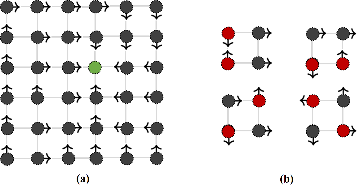
Figure 4: Subfigure (a) shows a bounded and direction preserving function in 2D, on a grid of size $6\times 6$. The fixed-point is shown in green. Several examples of patterns forbidden by the direction preserving property can be seen in subfigure (b).

For Brouwer we focus on constant rounds, since more than $\log{n}$ rounds do not improve the query complexity for Brouwer [CD05, CT07]. If the number of rounds is a non-constant function smaller than $\log{n}$, this only changes the bound by a sub-polynomial term.

Theorem 28.

(Brouwer fixed-point) Let $k$ be a constant. The query complexity of computing a discrete Brouwer fixed-point on the $d$-dimensional grid $[n]^{d}$ in $k$ rounds is $\Theta\left(n^{\frac{d^{k+1}-d^{k}}{d^{k}-1}}\right)$, for both deterministic and randomized algorithms.

Similarly to local search in constant rounds, when $k\rightarrow\infty$, this bound converges to $\Theta\left(n^{d-1}\right)$ and the gap is smaller than any polynomial. Thus our result fills the gap between one round algorithm and fully adaptive algorithm (logarithmic rounds) except for a small margin.

To compare the difficulty of problems under rounds limit on oracle evaluation, we use the round-preserving reduction defined as follow.

Definition 29 (round-preserving reduction).

A reduction from oracle-based problem P1 to oracle-based problem P2 is round-preserving if for any instance of problem P1 with oracle $\mathcal{O}_{1}$, the instance of problem P2 with oracle $\mathcal{O}_{2}$ given by the reduction satisfies that

1. A solution of the P1 instance can be obtained from any solution of the P2 instance without any more queries on $\mathcal{O}_{1}$.

2. Each query to $\mathcal{O}_{2}$ can be answered by a constant number of queries to $\mathcal{O}_{1}$ in one round.

The following lemma established the equivalence between the approximate and the discrete version of fixed-point problem.

Lemma 30 (see section 5 [CD05]).

1. There is a round-preserving reduction such that any instance $(\epsilon,L,d,F)$ of approximate fixed-point is reduced to an instance $(C_{1}(d)\cdot(L+1)/{\epsilon},d,f)$ of the discrete fixed-point problem, where $C_{1}(d)$ is a constant that only depends on the dimension $d$.

2. There is a round-preserving reduction with parameter $L>1$ such that any instance $(n,d,f)$ of discrete fixed-point problem is reduced to an instance $(\epsilon,L,d,F)$ of approximate fixed-point problem, satisfy that $((L-1)/\epsilon)\geq(C_{2}(d)\cdot n)$ where $C_{2}(d)$ is a constant that only depends on $d$.

Remark 1.

The original reduction from the discrete fixed-point problem to the approximate the version in [CD05] will take one more round of queries of the function $f$ of discrete fixed-point problem after getting the solution point $\mathbf{x}^{*}$ of approximate fixed-point problem. However, these extra queries can be avoided if $\epsilon$ is small enough. E.g., by taking $\epsilon=(L-1)/{(n\cdot d\cdot 2^{d})}$, the closest grid point (in $L_{\infty}$-norm) to the point $\mathbf{x}^{*}$ will be a zero point of $f$ under the construction in [CD05].

Since $d$ and $L$ are constants independent of $\epsilon$, we can study both the upper bound and lower bound of the discrete fixed-point problem first, then replace “$n$” with “$1/\epsilon$” to get the bound for the approximate fixed-point computing problem.

Theorem 3 (restated): Let $k\in\mathbb{N}$ be a constant. For any $\epsilon>0$, the query complexity of the $\epsilon$-approximate Brouwer fixed-point problem in the $d$-dimensional unit cube $[0,1]^{d}$ with $k$ rounds is $\Theta\left((1/\epsilon)^{\frac{d^{k+1}-d^{k}}{d^{k}-1}}\right)$, for both deterministic and randomized algorithms.

D.1 Upper Bound for Brouwer

Our constant rounds algorithm generalizes the divide-and-conquer algorithm in [CD05] in the same way as we generalizing the local search algorithm in [LTT93] in Section LABEL:sec:LS.ConstAlg. Therefore it is not surprising that we get the same upper bound for the discrete Brouwer fixed-point problem.

We first present several necessary definitions and lemmas in [CD05].

Definition 31 (bad cube, see definition 6 [CD05]).

A zero dimensional unit cube $C^{0}=\{\mathbf{x}\}$ is bad if $f(\mathbf{x})=\mathbf{e}^{1}$.

For each $i\geq 1$, an $i$-dimensional unit cube $C^{i}\subset[n]^{d}$ is bad with respect to function $f:[n]^{d}\rightarrow\{\mathbf{0},\pm\mathbf{e}^{1},\pm\mathbf{e}^{2},\ldots,\pm\mathbf{e}^{d}\}$ if

1. $\{f(\mathbf{x}):\mathbf{x}\in C^{i}\}=\{\mathbf{e}^{1},\mathbf{e}^{2},\ldots,\mathbf{e}^{i+1}\}$

2. the number of bad $(i-1)$-dimensional unit cubes in $C^{i}$ is odd.

The following theorem on the boundary condition of the existence of the solution is essential for the design of the divide-and-conquer based algorithm.

Theorem 32 (see Theorem 3 [CD05]).

A $(d-1)$-dimensional unit cube $C$ is on the boundary of a $d$-dimensional cube $C^{\prime}$ if every point in $C$ is on the boundary of $C^{\prime}$.

If the number of bad $(d-1)$-dimensional unit cubes on the boundary of the $d$-dimensional cube $C$ is odd, then the bounded direction-preserving function $f$ has a zero point within $C$.

The final piece that enables us to use a divide-and-conquer approach is that we can pad the original problem instance on the grid $[n]^{d}$ to a larger grid: $\{0,1,\ldots,n+1\}^{d}$, and make sure that the new instance contains exactly one bad $(d-1)$-dimensional unit cube on its boundary, and no new solution is introduced. Let $f$ and $f^{\prime}$ be the function for the original and the new instance, respectively. Then $f^{\prime}(\mathbf{x})=f(\mathbf{x})$ for any $\mathbf{x}\in[n]^{d}$; for any other point $\mathbf{x}=(x_{1},\ldots,x_{d})$, let $i$ be the largest number that $x_{i}\in\{0,n+1\}$, we have $f^{\prime}(\mathbf{x})=\mathbf{e}_{i}$ if $\mathbf{x}_{i}=0$ and $f^{\prime}(\mathbf{x})=-\mathbf{e}_{i}$ otherwise. The correctness of this reduction is showed in Lemma 5 of [CD05].

Algorithm for Brouwer.

1. Initialize the cube $C_{0}$ as $\{0,1,\ldots,n+1\}^{d}$; for each $0\leq i<k$, set $\ell_{i}=n^{\frac{d^{k}-d^{i}}{d^{k}-1}}$

2. In each round $i\in\{1,\ldots,k-1\}$:

   • Divide the current cube $C_{i-1}$ into sub-cubes $C_{i}^{1},\ldots,C_{i}^{n_{i}}$ of side length $\ell_{i}$ that cover $C_{i-1}$. These sub-cubes have mutually exclusive interior, but each $(d-1)$-dimensional unit cube that is not on the boundary of cube $C_{i-1}$ is either $(i)$ on the boundary of two sub-cubes $C_{i}^{j_{1}},C_{i}^{j_{2}}$ or $(ii)$ not on the boundary of any sub-cubes

   • Query $f^{\prime}$ with all the points on the boundary of sub-cubes $C_{i}^{1},\ldots,C_{i}^{n_{i}}$

   • Set $C_{i}=C_{i}^{j}$, where $C_{i}^{j}$ is the sub-cube that has odd number of bad $(d-1)$-dimensional unit cubes on its boundary. Choose arbitrary one if there are many

3. In round $k$, query all the points in the current cube $C_{k-1}$ and get the solution point.

Upper Bound of Theorem 28.

Notice that for any $i\in\{1,\ldots,k-1\}$, the sum of the numbers of bad $(d-1)$-dimensional cubes on the boundary of $C_{i}^{1},\ldots,C_{i}^{n_{i}}$ is still odd, since each bad cubes that is not on the boundary of $C_{i-1}$ is counted twice. By the parity argument, $C_{i}$ always exists. Finally, Lemma 32 guarantees that there exists a solution in cube $C_{k-1}$, which concludes the correctness of this algorithm.

The calculations in Section LABEL:sec:LS.ConstAlg imply that this algorithm makes $O\left(n^{\frac{d^{k+1}-d^{k}}{d^{k}-1}}\right)$ queries in total. ∎

D.2 Randomized Lower Bound for Brouwer

We reduce the local search instances generated by staircases to discrete Brouwer fixed-point instances in this section, and thus prove the lower bound part of Theorem 28.

We use the problem $GP$ defined in [CT07] as an intermediate problem in the reduction.

Definition 33 ($GP$, see section 2.2 [CT07]).

A graph directed $G=([n]^{d},E)$ is grid PPAD graph if

1. the underlying undirected graph of $G$ is a subgraph of grid graph defined on $[n]^{d}$;

2. there is one directed path $\mathbf{1}=\mathbf{x}_{0}\rightarrow\mathbf{x}_{1}\rightarrow\ldots\rightarrow\mathbf{x}_{T-1}\rightarrow\mathbf{x}_{T}$ with no self-intersection in the graph. Any other point outside of the path is an isolated point.

The structure of $G$ is accessed by the mapping function $N_{G}(\mathbf{x})$ from $[n]^{d}$ to $([n]^{d}\cup\{``no"\})\times([n]^{d}\cup\{``no^{\prime\prime}\})$, such that

1. $N_{G}(\mathbf{x}_{0})=(``no",\mathbf{x}_{1})$;

2. $N_{G}(\mathbf{x}_{T})=(\mathbf{x}_{T-1},``no")$;

3. $N_{G}(\mathbf{x}_{i})=(\mathbf{x}_{i-1},\mathbf{x}_{i+1})$, for all $i\in\{1,\ldots,T-1\}$;

4. $N_{G}(\mathbf{x})=(``no",``no")$, otherwise;

Then $GP$ is the following search problem: Given $n,d$ and the function $N_{G}(\mathbf{x})$, find the end of the path $\mathbf{x}_{T}$.

The following lemma in [CT07] shows that we can get the lower bound of discrete fixed-point problem from the lower bound of problem $GP$ directly.

Lemma 34 (see theorem 3.2 [CT07]).

There is a round-preserving reduction such that any instance $(n,d,N_{G})$ of problem $GP$ is reduced to an instance $(24n+7,d,f)$ of discrete fixed-point problem.

The remaining work is establishing the lower bound of problem $GP$ by reducing the local search instances generated by staircases to $GP$.

Lemma 35.

There is a round-preserving reduction such that any local search instance $(n,d,f)$ generated by possible staircase defined in Section B is reduced to an instance $(n,d,N_{G})$ of problem $GP$.

Proof.

Naturally, we can let the staircases in the local search instance to be the path in the $GP$ instance. Given a local search problem instance on grid $[n]^{d}$ with value function $f$ that is constructed by staircase as in Section B, we reduce it to a $GP$ instance on grid $[n]^{d}$ with function $N_{G}(\mathbf{x})$.

Each query of $N_{G}(\mathbf{x})$ is answered by at most $2d+1$ of queries of value function $f$ for $\mathbf{x}$ and all its neighbors. From these queries of $f$,

• if $f(\mathbf{x})>0$, let $\mathbf{x}$ be an isolated point, i.e., $N_{G}(\mathbf{x})=(``no",``no")$;

• otherwise, $\mathbf{x}$ should be on the path. If $f(\mathbf{x})=0$, $\mathbf{x}$ is the start of the path; if $\mathbf{x}$ is a local optima, $\mathbf{x}$ is the end of the path. The direction within the paths is from the point with higher value to the point with lower value, and there are at most one neighbor with higher value and at most one neighbor with lower value for any value function $f$ constructed in Section B. Thus we can answer $N_{G}(\mathbf{x})$ correctly by the values of $\mathbf{x}$ and its neighbor.

Since the start point and the end point of a staircase are unique under the construction in Section B, $\mathbf{x}_{T}$ is the solution of the original local search problem, and the start of the path $\mathbf{x}_{0}$ satisfies $\mathbf{x}_{0}=\mathbf{1}$. This reduction does not change the number of rounds needed, and only increases the number of queries by a constant factor $2d+1$. Thus the reduction above is a round-preserving reduction. ∎

Combining Lemma 34, Lemma 35, and Theorem 1 concludes the proof of the lower bound in Theorem 28.

Appendix E Local Search and Brouwer Fixed-Point in 1D

In this section we study the local search and discrete Brouwer fixed-point on one dimensional grid.

Recall that the white-box version (where the function is given by a polynomial size circuit) of local search is PLS-Complete for any $d\geq 2$. On the other hand, when $d=1$, a binary search procedure can solve the problem with $O(\log n)$ queries. Therefore, the query complexity in the 1-dimensional case exhibits different properties than that in dimension $d\geq 2$.

Theorem 36.

(1-dimensional case) Let $k$ be a constant. The query complexity of computing a local minimum on the $1$-dimensional grid $[n]$ in $k$ rounds is $\Theta\left(n^{1/k}\right)$, for both deterministic and randomized algorithms.

Note that in the fully adaptive case, the query complexity of this problem is $\Theta\left(\log n\right)$.

We have similar results for Brouwer. Here we are given a function $f:[0,1]\to[0,1]$ with Lipschitz constant $L>1$ and a parameter $\epsilon>0$ and the goal is to find an $\epsilon$-approximate fixed point of $f$. We first show a bound for the discrete Brouwer problem, which will imply a tight bound for the continuous setting.

Theorem 37.

(Discrete Brouwer in 1D) Let $k$ be a constant. Given a bounded and direction-preserving function $f:[n]\to[n]$, the query complexity of computing a discrete Brouwer fixed point in $k$ rounds is $\Theta\left(n^{1/k}\right)$, for both deterministic and randomized algorithms.

Corollary 38.

(Brouwer in 1D) Let $k$ be a constant. Given a $L$-Lipschitz continuous function $f:[0,1]\to[0,1]$ with $L>1$ and $\epsilon>0$, the query complexity of computing an $\epsilon$-approximate fixed point of $f$ in $k$ rounds is $\Theta\left((1/\epsilon)^{1/k}\right)$, for both deterministic and randomized algorithms.

Note that in the fully adaptive case, the query complexity of this problem is $\Theta\left(\log 1/\epsilon\right)$.

We conclude the proof of Theorem 36 and Theorem 37 by a deterministic algorithm in Section E.1 and a matching lower bound for randomized algorithm in Section E.2.

E.1 Algorithm in 1D

The algorithm is a simple adaptation of previous constant rounds algorithms into 1D.

Algorithm in constant rounds in 1D

1. Initialize the current interval as $[n]$.

2. In each round $i\in\{1,\ldots,k-1\}$:

   • Divide the current interval into $n^{1/k}$ of mutually exclusive sub-intervals, and query all the points on the boundary of these sub-intervals.

   • For local search, set the current interval to be the sub-interval with minimum value in it; for Brouwer, set the current interval to be the one has a fixed-point or both boundary points pointing inwards. Break tie arbitrarily.

3. In round $k$, query all the points in the current interval and find the solution point.

Upper Bound of Theorem 36 and Theorem 37.

The correctness of the algorithm follows from similar argument as the $d\geq 2$ case: for local search, the steepest descent from the minimal point will not escape from the current sub-interval; for Brouwer, the direction-preserving function in 1D can not change its direction without stopping at a fixed-point.

The total number of queries is at most $(k-1)\cdot 2n^{1/k}+n^{1/k}=O(n^{1/k})$. ∎

E.2 Lower Bound in 1D

Lower Bound of Theorem 36 and Theorem 37.

By Yao’s minimax theorem, we first construct a distribution of hard instances and then use standard decision tree method to show that $O(n^{1/k})$ queries are necessary for any deterministic algorithm.

Hard Local Search Instances

A uniform distribution over $n$ possible instances $f_{1},\ldots,f_{n}$, where $f_{i}$ is defined as below:

1. $f_{i}(i)=0$;

2. $f_{i}(j)=j$, if $j>i$;

3. $f_{i}(j)=n-j+1$, if $j<i$

The only solution of $f_{i}$ is the point $i$. A second observation is that for any set of $q$ queries points, there are at most $2q+1$ possible results considering all $f_{i}$, because there are at most $2q+1$ of possible different relative location between the $q$ queried points.

Now consider the decision tree of any $k$-rounds deterministic algorithm $A$. If the number of queries on every node are $o(n^{1/k})$, the number of leaf node are $o(n)$, i.e., the algorithm $A$ will fail with high probability.

Hard Discrete Brouwer Fixed-Point Instances

A uniform distribution over $n$ possible instances $f_{1},\ldots,f_{n}$, where $f_{i}$ is defined as below:

1. $f_{i}(i)=0$;

2. $f_{i}(j)=-1$, if $j>i$;

3. $f_{i}(j)=1$, if $j<i$

Any function $f_{i}$ is bounded and direction-preserving, and the only solution is point $i$. The remaining proof is exactly same as the local search. Therefore, we conclude that $\Omega(n^{1/k})$ queries are necessary for any $k$ rounds algorithm for local search or Brouwer in 1D.

∎

References

- [Aar06] Scott Aaronson. Lower bounds for local search by quantum arguments. SIAM Journal on Computing, 35(4):804–824, 2006.
- [AAV86] Noga Alon, Yossi Azar, and Uzi Vishkin. Tight complexity bounds for parallel comparison sorting. In 27th Annual Symposium on Foundations of Computer Science (sfcs 1986), pages 502–510. IEEE, 1986.
- [AK93] Ingo Althöfer and Klaus-Uwe Koschnick. On the deterministic complexity of searching local maxima. Discret. Appl. Math., 43(2):111–113, 1993.
- [Akl14] Selim Akl. Parallel Sorting Algorithms. Academic Press, 2014.
- [Ald83] David Aldous. Minimization algorithms and random walk on the -cube. The Annals of Probability, 11(2):403–413, 1983.
- [BM20] Sébastien Bubeck and Dan Mikulincer. How to trap a gradient flow. In Conference on Learning Theory, COLT 2020, 9-12 July 2020, Virtual Event [Graz, Austria], volume 125 of Proceedings of Machine Learning Research, pages 940–960. PMLR, 2020.
- [BMP19] Mark Braverman, Jieming Mao, and Yuval Peres. Sorted top-k in rounds. In Alina Beygelzimer and Daniel Hsu, editors, Conference on Learning Theory, COLT 2019, 25-28 June 2019, Phoenix, AZ, USA, volume 99 of Proceedings of Machine Learning Research, pages 342–382. PMLR, 2019.
- [BMW16] Mark Braverman, Jieming Mao, and S. Matthew Weinberg. Parallel algorithms for select and partition with noisy comparisons. In Daniel Wichs and Yishay Mansour, editors, Proceedings of the 48th Annual ACM SIGACT Symposium on Theory of Computing, STOC 2016, Cambridge, MA, USA, June 18-21, 2016, pages 851–862. ACM, 2016.
- [Bol88] Béla Bollobás. Sorting in rounds. Discrete Mathematics, 72(1-3):21–28, 1988.
- [Bro10] L.E.J. Brouwer. Continuous one-one transformations of sur-faces in themselves. Koninklijke Neder-landse Akademie van Weteschappen, Proceedings Series B Physical Sciences, 13:967–977, 1910.
- [Bro11] L.E.J. Brouwer. Continuous one-one transformations of surfaces in themselves. Koninklijke Neder-landse Akademie van Weteschappen Proceedings Series B Physical Sciences, 14:300–310, 1911.
- [BS18] Eric Balkanski and Yaron Singer. The adaptive complexity of maximizing a submodular function. In Ilias Diakonikolas, David Kempe, and Monika Henzinger, editors, Proceedings of the 50th Annual ACM SIGACT Symposium on Theory of Computing, Los Angeles, CA, USA, June 25-29, 2018, pages 1138–1151. ACM, 2018.
- [CD05] Xi Chen and Xiaotie Deng. On algorithms for discrete and approximate brouwer fixed points. In Proceedings of the thirty-seventh annual ACM symposium on Theory of computing, pages 323–330, 2005.
- [CD09] Xi Chen and Xiaotie Deng. On the complexity of 2d discrete fixed point problem. Theor. Comput. Sci., 410(44):4448–4456, 2009.
- [CDT09] Xi Chen, Xiaotie Deng, and Shang-Hua Teng. Settling the complexity of computing two-player nash equilibria. J. ACM, 56(3):14:1–14:57, 2009.
- [CMM20] Vincent Cohen-Addad, Frederik Mallmann-Trenn, and Claire Mathieu. Instance-optimality in the noisy value-and comparison-model. In Shuchi Chawla, editor, Proceedings of the 2020 ACM-SIAM Symposium on Discrete Algorithms, SODA 2020, Salt Lake City, UT, USA, January 5-8, 2020, pages 2124–2143. SIAM, 2020.
- [CPY17] Xi Chen, Dimitris Paparas, and Mihalis Yannakakis. The complexity of non-monotone markets. J. ACM, 64(3):20:1–20:56, 2017.
- [CT07] Xi Chen and Shang-Hua Teng. Paths beyond local search: A tight bound for randomized fixed-point computation. In 48th Annual IEEE Symposium on Foundations of Computer Science (FOCS’07), pages 124–134. IEEE, 2007.
- [DGP09] Constantinos Daskalakis, Paul W. Goldberg, and Christos H. Papadimitriou. The complexity of computing a nash equilibrium. SIAM J. Comput., 39(1):195–259, 2009.
- [DP11] Constantinos Daskalakis and Christos H. Papadimitriou. Continuous local search. In Dana Randall, editor, Proceedings of the Twenty-Second Annual ACM-SIAM Symposium on Discrete Algorithms, SODA 2011, San Francisco, California, USA, January 23-25, 2011, pages 790–804. SIAM, 2011.
- [DSZ21] Constantinos Daskalakis, Stratis Skoulakis, and Manolis Zampetakis. The complexity of constrained min-max optimization. In Proceedings of the ACM Symposium on Theory of Computing. Association for Computing Machinery, 2021.
- [FGHS21] John Fearnley, Paul W. Goldberg, Alexandros Hollender, and Rahul Savani. The complexity of gradient descent: CLS = PPAD PLS. In Proceedings of the ACM Symposium on Theory of Computing. Association for Computing Machinery, 2021.
- [FPT04] Alex Fabrikant, Christos H. Papadimitriou, and Kunal Talwar. The complexity of pure nash equilibria. In László Babai, editor, Proceedings of the 36th Annual ACM Symposium on Theory of Computing, Chicago, IL, USA, June 13-16, 2004, pages 604–612. ACM, 2004.
- [GGK03a] William Gasarch, Evan Golub, and Clyde Kruskal. Constant time parallel sorting: an empirical view. Journal of Computer and System Sciences, 67(1):63–91, 2003.
- [GGK03b] William I. Gasarch, Evan Golub, and Clyde P. Kruskal. Constant time parallel sorting: an empirical view. J. Comput. Syst. Sci., 67(1):63–91, 2003.
- [HPV89] Michael D Hirsch, Christos H Papadimitriou, and Stephen A Vavasis. Exponential lower bounds for finding brouwer fix points. Journal of Complexity, 5(4):379–416, 1989.
- [HY17] Pavel Hubáček and Eylon Yogev. Hardness of continuous local search: Query complexity and cryptographic lower bounds. In Proceedings of the Twenty-Eighth Annual ACM-SIAM Symposium on Discrete Algorithms, pages 1352–1371. SIAM, 2017.
- [Iim03] Takuya Iimura. A discrete fixed point theorem and its applications. Journal of Mathematical Economics, 39(7):725–742, 2003.
- [JPY88] David S. Johnson, Christos H. Papadimitriou, and Mihalis Yannakakis. How easy is local search? J. Comput. Syst. Sci., 37(1):79–100, 1988.
- [LL10] Gregory F Lawler and Vlada Limic. Random walk: a modern introduction, volume 123. Cambridge University Press, 2010.
- [LT93] Donna Crystal Llewellyn and Craig A. Tovey. Dividing and conquering the square. Discret. Appl. Math., 43(2):131–153, 1993.
- [LTT93] Donna Crystel Llewellyn, Craig Tovey, and Michael Trick. Local optimization on graphs: Discrete applied mathematics 23 (1989) 157–178. Discrete Applied Mathematics, 46(1):93–94, 1993.
- [Nem94] A. Nemirovski. On parallel complexity of nonsmooth convex optimization. Journal of Complexity, 10(4):451 – 463, 1994.
- [Pap94] Christos H. Papadimitriou. On the complexity of the parity argument and other inefficient proofs of existence. J. Comput. Syst. Sci., 48(3):498–532, 1994.
- [Pip87] Nicholas Pippenger. Sorting and selecting in rounds. SIAM Journal on Computing, 16(6):1032–1038, 1987.
- [Set12] Burr Settles. Active learning. Synthesis Lectures on Artificial Intelligence and Machine Learning, 6(1):1–114, 2012.
- [SY91] Alejandro A. Schäffer and Mihalis Yannakakis. Simple local search problems that are hard to solve. SIAM J. Comput., 20(1):56–87, 1991.
- [SY09] Xiaoming Sun and Andrew Chi-Chih Yao. On the quantum query complexity of local search in two and three dimensions. Algorithmica, 55(3):576–600, 2009.
- [Tov81] Craig Tovey. Polynomial local improvement algorithms in combinatorial optimization, 1981. Ph.D. thesis, Stanford University.
- [Val75] Leslie G. Valiant. Parallelism in comparison problems. SIAM Journal on Computing, 4(3):348–355, 1975.
- [Vav93] Stephen A Vavasis. Black-box complexity of local minimization. SIAM Journal on Optimization, 3(1):60–80, 1993.
- [VY11] Vijay V. Vazirani and Mihalis Yannakakis. Market equilibrium under separable, piecewise-linear, concave utilities. J. ACM, 58(3):10:1–10:25, 2011.
- [WZ99] Avi Wigderson and David Zuckerman. Expanders that beat the eigenvalue bound: Explicit construction and applications. Combinatorica, 19(1):125–138, 1999.
- [Yao77] Andrew Yao. Probabilistic computations: Toward a unified measure of complexity. In Proceedings of the 18th IEEE Symposium on Foundations of Computer Science (FOCS), pages 222–227, 1977.
- [Zha09] Shengyu Zhang. Tight bounds for randomized and quantum local search. SIAM Journal on Computing, 39(3):948–977, 2009.