Conflict-driven Inductive Logic Programming

Abstract

The goal of Inductive Logic Programming (ILP) is to learn a program that explains a set of examples. Until recently, most research on ILP targeted learning Prolog programs. The ILASP system instead learns Answer Set Programs (ASP). Learning such expressive programs widens the applicability of ILP considerably; for example, enabling preference learning, learning common-sense knowledge, including defaults and exceptions, and learning non-deterministic theories.

Early versions of ILASP can be considered meta-level ILP approaches, which encode a learning task as a logic program and delegate the search to an ASP solver. More recently, ILASP has shifted towards a new method, inspired by conflict-driven SAT and ASP solvers. The fundamental idea of the approach, called Conflict-driven ILP (CDILP), is to iteratively interleave the search for a hypothesis with the generation of constraints which explain why the current hypothesis does not cover a particular example. These coverage constraints allow ILASP to rule out not just the current hypothesis, but an entire class of hypotheses that do not satisfy the coverage constraint.

This paper formalises the CDILP approach and presents the ILASP3 and ILASP4 systems for CDILP, which are demonstrated to be more scalable than previous ILASP systems, particularly in the presence of noise.

Under consideration in Theory and Practice of Logic Programming (TPLP).

1 Introduction

Inductive Logic Programming (ILP) [Muggleton (1991)] systems aim to find a set of logical rules, called a hypothesis, that, together with some existing background knowledge, explain a set of examples. Unlike most ILP systems, which usually aim to learn Prolog programs, the ILASP (Inductive Learning of Answer Set Programs) systems [Law et al. (2014), Law (2018), Law et al. (2020)] can learn Answer Set Programs (ASP), including normal rules, choice rules, disjunctive rules, and hard and weak constraints. ILASP’s learning framework has been proven to generalise existing frameworks and systems for learning ASP programs [Law et al. (2018a)], such as the brave learning framework [Sakama and Inoue (2009)], adopted by almost all previous systems (e.g. XHAIL [Ray (2009)], ASPAL [Corapi et al. (2011)], ILED [Katzouris et al. (2015)], RASPAL [Athakravi et al. (2013)]), and the less common cautious learning framework [Sakama and Inoue (2009)]. Brave systems require the examples to be covered in at least one answer set of the learned program, whereas cautious systems find a program which covers the examples in every answer set. The results in [Law et al. (2018a)] show that some ASP programs cannot be learned with either a brave or a cautious approach, and that to learn ASP programs in general, a combination of both brave and cautious reasoning is required. ILASP’s learning framework enables this combination, and is capable of learning the full class of ASP programs [Law et al. (2018a)]. ILASP’s generality has allowed it to be applied to a wide range of applications, including event detection [Law et al. (2018b)], preference learning [Law et al. (2015)], natural language understanding [Chabierski et al. (2017)], learning game rules [Cropper et al. (2020)], grammar induction [Law et al. (2019)] and automata induction [Furelos-Blanco et al. (2020), Furelos-Blanco et al. (2021)].

Throughout the last few decades, ILP systems have evolved from early bottom-up/top-down learners, such as [Quinlan (1990), Muggleton (1995), Srinivasan (2001)], to more modern systems, such as [Cropper and Muggleton (2016), Kaminski et al. (2019), Corapi et al. (2010), Corapi et al. (2011)], which take advantage of logic programming systems to solve the task. These recent ILP systems, commonly referred to as meta-level systems, work by transforming an ILP learning problem into a meta-level logic program whose solutions can be mapped back to the solutions of the original ILP problem. The specific notion of solution of the meta-level logic program differs from system to system, but to give an example, in ASPAL a brave induction task is mapped into an ASP program whose answer sets each encode a brave inductive solution of the original task. When compared to older style bottom-up/top-down learners, the advantage of meta-level approaches is that they tend to be complete (which means that most systems are guaranteed to find a solution if one exists) and because they use off-the-shelf logic programming systems to perform the search for solutions, problems which had previously been difficult challenges for ILP (such as recursion and non-observational predicate learning) are much simpler. Unlike traditional ILP approaches, which incrementally construct a hypothesis based on a single seed example at a time, meta-level ILP systems tend to be batch learners and consider all examples at once. This can mean that they lack scalability on datasets with large numbers of examples.

At first glance, the earliest ILASP systems (ILASP1 [Law et al. (2014)] and ILASP2 [Law et al. (2015)]) may seem to be meta-level systems, and they do indeed involve encoding a learning task as a meta-level ASP program; however, they are actually in a more complicated category. Unlike “pure” meta-level systems, the ASP solver is not invoked on a fixed program, and is instead (through the use of multi-shot solving [Gebser et al. (2016)]) incrementally invoked on a program that is growing throughout the execution. With each new version, ILASP has shifted further away from pure meta-level approaches, towards a new category of ILP system, which we call conflict-driven. Conflict-driven ILP systems, inspired by conflict-driven SAT and ASP solvers, iteratively construct a set of constraints on the solution space that must be satisfied by any inductive solution. In each iteration, the solver finds a program $H$ that satisfies the current constraints, then searches for a conflict $C$, which corresponds to a reason why $H$ is not an (optimal) inductive solution. If none exists, then $H$ is returned; otherwise, $C$ is converted to a new coverage constraint which the next programs must satisfy. The process of converting a conflict into a new coverage constraint is called conflict analysis.

This paper formalises the notion of Conflict-driven Inductive Logic Programming (CDILP) which is at the core of the most recent two ILASP systems (ILASP3 [Law (2018)] and ILASP4). Although ILASP3 was released in 2017 and previously presented in Mark Law’s PhD thesis [Law (2018)], and has been evaluated on several applications [Law et al. (2018b)], the approach has not been formally published until now. In fact, despite being equivalent to the formalisation in this paper, the definition of ILASP3 in [Law (2018)] uses very different terminology.

This paper first presents CDILP at an abstract level and proves that, assuming certain guarantees are met, any instantiation of CDILP is guaranteed to find an optimal solution for any learning task, provided at least one solution exists. ILASP3 and ILASP4 are both instances of the CDILP aproach, with the difference being their respective methods for performing conflict analysis. These are formalised in Section 4, with a discussion of the strengths and weaknesses of each method. In particular, we identify one type of learning task on which ILASP4 is likely to significantly outperform ILASP3.

CDILP is shown through an evaluation to be significantly faster than previous ILASP systems on tasks with noisy examples. One of the major advantages of the CDILP approach is that it allows for constraint propagation, where a coverage constraint computed for one example is propagated to another example. This means that the conflict analysis performed on one example does not need to be repeated for other similar examples, thus improving efficiency.

The CDILP approach (as ILASP3) has already been evaluated [Law et al. (2018b)] on several real datasets and compared with other state-of-the-art ILP systems. Unlike ILASP, these systems do not guarantee finding an optimal solution of the learning task (in terms of the length of the hypothesis, and the penalties paid for not covering examples). ILASP finds solutions which are on average better quality than those found by the other systems (in terms of the $F_{1}$-score on a test set of examples) [Law et al. (2018b)]. The evaluation in this paper compares the performance of ILASP4 to ILASP3 on several synthetic learning tasks, and shows that ILASP4 is often significantly faster than ILASP3.

The CDILP framework is entirely modular, meaning that users of the ILASP system can replace any part of the CDILP approach with their own method; for instance, they could define a new method for conflict analysis or constraint propagation to increase performance in their domain. Providing their new method shares the same correctness properties as the original modules in ILASP, their customised CDILP approach will still be guaranteed to terminate and find an optimal solution. This customisation is supported in the ILASP implementation through the use of a new Python interface (called PyLASP).

The rest of the paper is structured as follows. Section 2 recalls the necessary background material. Section 3 formalises the notion of Conflict-driven ILP. Section 4 presents several approaches to conflict analysis. Section 5 gives an evaluation of the approach. Finally, Sections 6 and 7 present the related work and conclude the paper.

2 Background

This section introduces the background material that is required to understand the rest of the paper. First, the fundamental Answer Set Programming concepts are recalled, and then the learning from answer sets framework used by the ILASP systems is formalised.

2.1 Answer Set Programming

A disjunctive rule $R$ is of the form $\mathtt{h_{1}\lor\ldots\lor h_{m}\texttt{:- }b_{1},\ldots,b_{n},}$ $\mathtt{\texttt{not }c_{1},\ldots,\texttt{not }c_{o}}$, where $\{\mbox{$\mathtt{h_{1}}$},\ldots,\mbox{$\mathtt{h_{m}}$}\}$, $\{\mbox{$\mathtt{b_{1}}$},\ldots,\mbox{$\mathtt{b_{n}}$}\}$ and $\{\mbox{$\mathtt{c_{1}}$},\ldots,\mbox{$\mathtt{c_{o}}$}\}$ are sets of atoms denoted $\textit{head}(R)$, $\textit{body}^{\mathchar 43\relax}(R)$ and $\textit{body}^{\mathchar 45\relax}(R)$, respectively. A normal rule $R$ is a disjunctive rule such that $|\textit{head}(R)|\mathchar 61\relax 1$. A definite rule $R$ is a disjunctive rule such that $|\textit{head}(R)|\mathchar 61\relax 1$ and $|\textit{body}^{\mathchar 45\relax}(R)|\mathchar 61\relax 0$. A hard constraint $R$ is a disjunctive rule such that $|\textit{head}(R)|\mathchar 61\relax 0$. Sets of disjunctive, normal and definite rules are called disjunctive, normal and definite logic programs (respectively).

Given a (First-order) disjunctive logic program $P$, the Herbrand base ($\textit{HB}_{P}$) is the set of all atoms constructed using constants, functions and predicates in $P$. The program $\textit{ground}(P)$ is constructed by replacing each rule with its ground instances (using only atoms from the Herbrand base). An (Herbrand) interpretation $I$ (of $P$) assigns each element of $\textit{HB}_{P}$ to $\mathtt{\top}$ or $\mathtt{\bot}$, and is usually written as the set of all elements in $\textit{HB}_{P}$ that $I$ assigns to $\mathtt{\top}$. An interpretation $I$ is a model of $P$ if it satisfies every rule in $P$; i.e. for each rule $R\in\textit{ground}(P)$ if $\textit{body}^{\mathchar 43\relax}(R)\subseteq I$ and $\textit{body}^{\mathchar 45\relax}(R)\cap I\mathchar 61\relax\emptyset$ then $\textit{head}(R)\cap I\neq\emptyset$. A model of $P$ is minimal if no strict subset of $P$ is also a model of $P$. The reduct of $P$ wrt $I$ (denoted $P^{I}$) is the program constructed from $\textit{ground}(P)$ by first removing all rules $R$ such that $\textit{body}^{\mathchar 45\relax}(R)\cap I\neq\emptyset$ and then removing all remaining negative body literals from the program. The answer sets of $P$ are the interpretations $I$ such that $I$ is a minimal model of $P^{I}$. The set of all answer sets of $P$ is denoted $\textit{AS}(P)$.

There is another way of characterising answer sets, by using unfounded subsets. Let $P$ be a disjunctive logic program and $I$ be an interpretation. A subset $U\subseteq I$ is unfounded (w.r.t. $P$) if there is no rule $R\in\textit{ground}(P)$ for which the following three conditions all hold: (1) $\textit{head}(R)\cap I\subseteq U$; (2) $\textit{body}^{\mathchar 43\relax}(R)\subseteq I\backslash U$; and (3) $\textit{body}^{\mathchar 45\relax}(R)\cap I\mathchar 61\relax\emptyset$. The answer sets of a program $P$ are the models of $P$ with no non-empty unfounded subsets w.r.t. $P$.

Unless otherwise stated, in this paper the term ASP program is used to mean a program consisting of a finite set of disjunctive rules.

2.2 Learning from Answer Sets

The Learning from Answer Sets framework, introduced in [Law et al. (2014)], is targeted at learning ASP programs. The basic framework has been extended several times, allowing learning weak constraints [Law et al. (2015)], learning from context-dependent examples [Law et al. (2016)] and learning from noisy examples [Law et al. (2018b)]. This section presents the $\textit{ILP}_{\textit{\scriptsize LAS}}^{\textit{ \scriptsize noise}}$ learning framework, which is used in this paper.

Examples in $\textit{ILP}_{\textit{\scriptsize LAS}}^{\textit{ \scriptsize noise}}$ are Context-dependent Partial Interpretations (CDPIs). CDPIs specify what should or should not be an answer set of the learned program. A partial interpretation $e_{\mathit{pi}}$ is a pair of sets of atoms $\langle e^{\mathit{inc}},e^{\mathit{exc}}\rangle$ called the inclusions and the exclusions, respectively. An interpretation $I$ extends $e_{\mathit{pi}}$ if and only if $e^{\mathit{inc}}\subseteq I$ and $e^{\mathit{exc}}\cap I\mathchar 61\relax\emptyset$. A Context-dependent Partial Interpretation $e$ is a pair $\langle e_{\mathit{pi}},e_{\mathit{ctx}}\rangle$ where $e_{\mathit{pi}}$ is a partial interpretation and $e_{\mathit{ctx}}$ (the context of $e$) is a disjunctive logic program. A program $P$ is said to accept $e$ if there is at least one answer set $A$ of $P\cup e_{\mathit{ctx}}$ that extends $e_{\mathit{pi}}$ – such an $A$ is called an accepting answer set of $e$ w.r.t. $P$, written $A\in\textit{AAS}(e,P)$.

Example 1

Consider the program $P$, with the following two rules:

heads(V1) :- coin(V1), not tails(V1).
tails(V1) :- coin(V1), not heads(V1).

• $P$ accepts $e\mathchar 61\relax\langle\langle\{\mbox{$\mathtt{heads(c1)}$}\},\{\mbox{$\mathtt{tails(c1)}$}\}\rangle,\{\mbox{$\mathtt{coin(c1)\texttt{.}}$}\}\rangle$. The only accepting answer set of $e$ w.r.t. $P$ is $\{\mbox{$\mathtt{heads(c1)}$},\mbox{$\mathtt{coin(c1)}$}\}$.

• $P$ accepts $e\mathchar 61\relax\langle\langle\{\mbox{$\mathtt{heads(c1)}$}\}$, $\{\mbox{$\mathtt{tails(c1)}$}\}\rangle,\{\mbox{$\mathtt{coin(c1)\texttt{.}\;\;coin(c2)\texttt{.}}$}\}\rangle$. The two accepting answer sets of $e$ w.r.t. $P$ are $\{\mbox{$\mathtt{heads(c1)}$}$, $\mathtt{heads(c1)}$, $\mathtt{coin(c1)}$, $\mbox{$\mathtt{coin(c2)}$}\}$ and $\{\mbox{$\mathtt{heads(c1)}$}$, $\mathtt{tails(c1)}$, $\mathtt{coin(c1)}$, $\mbox{$\mathtt{coin(c2)}$}\}$.

• $P$ does not accept $e\mathchar 61\relax\langle\langle\{\mbox{$\mathtt{heads(c1)}$},\mbox{$\mathtt{tails(c1)}$}\},\emptyset\rangle,\{\mbox{$\mathtt{coin(c1)\texttt{.}}$}\}\rangle$.

• $P$ does not accept $e\mathchar 61\relax\langle\langle\{\mbox{$\mathtt{heads(c1)}$}\},\{\mbox{$\mathtt{tails(c1)}$}\}\rangle,\emptyset\rangle$.

In learning from answer sets tasks, CDPIs are given as either positive (resp. negative) examples, which should (resp. should not) be accepted by the learned program.

Noisy examples.

In settings where all examples are correctly labelled (i.e. there is no noise), ILP systems search for a hypothesis that covers all of the examples. Many systems search for the optimal such hypothesis – this is usually defined as the hypothesis minimising the number of literals in $H$ ($|H|$). In real settings, examples are often not guaranteed to be correctly labelled. In these cases, many ILP systems (including ILASP) assign a penalty to each example, which is the cost of not covering the example. A CDPI $e$ can be upgraded to a weighted CDPI by adding a penalty $e_{\mathit{pen}}$, which is either a positive integer or $\infty$, and a unique identifier, $e_{\mathit{id}}$, for the example.

Learning Task.

Definition 7 formalises the $\textit{ILP}_{\textit{\scriptsize LAS}}^{\textit{ \scriptsize noise}}$ learning task, which is the input of the ILASP systems. A rule space $S_{M}$ (often called a hypothesis space and characterised by a mode bias $M$) is a finite set of disjunctive rules, defining the space of programs that are allowed to be learned. Given a rule space $S_{M}$, a hypothesis $H$ is any subset of $S_{M}$. The goal of a system for $\textit{ILP}_{\textit{\scriptsize LAS}}^{\textit{ \scriptsize noise}}$ is to find an optimal inductive solution $H$, which is a subset of a given rule space $S_{M}$, that covers every example with infinite penalty and minimises the sum of the length of $H$ plus the penalty of each uncovered example.

Definition 1

An $\textit{ILP}_{\textit{\scriptsize LAS}}^{\textit{ \scriptsize noise}}$ task $T$ is a tuple of the form $\langle B,S_{M},\langle E^{\mathchar 43\relax},E^{\mathchar 45\relax}\rangle\rangle$, where $B$ is an ASP program called the background knowledge, $S_{M}$ is a rule space and $E^{\mathchar 43\relax}$ and $E^{\mathchar 45\relax}$ are (finite) sets of weighted CDPIs. Given a hypothesis $H\subseteq S_{M}$,

1. $\mathcal{U}(H,T)$ is the set consisting of: (a) all positive examples $e\in E^{\mathchar 43\relax}$ such that $B\cup H$ does not accept $e$; and (b) all negative examples $e\in E^{\mathchar 45\relax}$ such that $B\cup H$ accepts $e$.

2. the score of $H$, denoted as $\mathcal{S}(H,T)$, is the sum $|H|\mathchar 43\relax\sum_{e\in\mathcal{U}(H,T)}e_{pen}$.

3. $H$ is an inductive solution of $T$ (written $H\in\textit{ILP}_{\textit{\scriptsize LAS}}^{\textit{ \scriptsize noise}}(T)$) if and only if $\mathcal{S}(H,T)$ is finite (i.e. $H$ must cover all examples with infinite penalty).

4. $H$ is an optimal inductive solution of $T$ (written $H\in$ ${}^{*}\textit{ILP}_{\textit{\scriptsize LAS}}^{\textit{ \scriptsize noise}}(T)$) if and only if $\mathcal{S}(H,T)$ is finite and $\nexists H^{\prime}\subseteq S_{M}$ such that $\mathcal{S}(H,T)\mathchar 62\relax\mathcal{S}(H^{\prime},T)$.

3 Conflict-driven Inductive Logic Programming

In this section, we present ILASP’s Conflict-driven ILP (CDILP) algorithm. For simplicity, we first explain how the CDILP approach solves non-noisy learning tasks. In this case, the CDILP process iteratively builds a set of coverage constraints for each example, which specify certain conditions for that example to be covered. In each iteration, the CDILP process computes an optimal hypothesis $H^{*}$ (i.e. a hypothesis which is as short as possible) that conforms to the existing coverage constraints; it then searches for an example that is not covered by $H^{*}$ and computes a new coverage constraint for that example – esentially, this can be viewed as an explanation of why $H^{*}$ is not an inductive solution. Eventually, the CDILP process reaches an iteration where the hypothesis $H^{*}$ covers every example. In this (final) iteration, $H^{*}$ is returned as the optimal solution of the task. The noisy case is slightly more complicated. Firstly, the computed optimal hypothesis $H^{*}$ does not need to cover every example and, therefore, does not need to conform to every coverage constraint. Instead, $H^{*}$ must be optimal in terms of its length plus the penalties of all examples for which $H^{*}$ does not cover at least one existing coverage constraint – essentially, this search “chooses” not to cover certain examples. Secondly, the search for an uncovered example must find an example that the hypothesis search did not “choose” not to cover (i.e. an uncovered example $e$ such that $H^{*}$ conforms to every existing coverage constraint for $e$).

Roughly speaking, coverage constraints are boolean constraints over the rules that a hypothesis must contain to cover a particular example; for example, they may specify that a hypothesis must contain at least one of a particular set of rules and none of another set of rules. The coverage constraints supported by ILASP are formalised by Definition 2. Throughout the rest of the paper, we assume $T\mathchar 61\relax\langle B,S_{M},E\rangle$ to be an $ILP_{LAS}^{noise}$ learning task. We also assume that every rule $R$ in $S_{M}$ has a unique identifier, written $R_{\mathit{id}}$.

Definition 2

Let $S_{M}$ be a rule space. A coverage formula over $S_{M}$ takes one of the following forms:

• $R_{id}$, for some $R\in S_{M}$.

• $\lnot F$, where $F$ is a coverage formula over $S_{M}$.

• $F_{1}\lor\ldots\lor F_{n}$, where $F_{1},\ldots,F_{n}$ are coverage formulas over $S_{M}$.

• $F_{1}\land\ldots\land F_{n}$, where $F_{1},\ldots,F_{n}$ are coverage formulas over $S_{M}$.

The semantics of coverage formulas are defined as follows. Given a hypothesis $H$:

• $R_{id}$ accepts $H$ if and only if $R\in H$.

• $\lnot F$ accepts $H$ if and only if $F$ does not accept $H$.

• $F_{1}\lor\ldots\lor F_{n}$ accepts $H$ if and only if $\exists i\in[1,n]$ s.t. $F_{i}$ accepts $H$.

• $F_{1}\land\ldots\land F_{n}$ accepts $H$ if and only if $\forall i\in[1,n]$ s.t. $F_{i}$ accepts $H$.

A coverage constraint is a pair $\langle e,F\rangle$, where $e$ is an example in $E$ and $F$ is a coverage formula, such that for any $H\subseteq S_{M}$, if $e$ is covered then $F$ accepts $H$.

Example 2

Consider a task with background knowledge $B$ and the following rule space $S_{M}$:

$\left\{\begin{array}[]{llllll}h^{1}:&\mbox{}\mbox{$\mathtt{heads\texttt{.}}$}&\mbox{}h^{2}:&\mbox{}\mbox{$\mathtt{tails\texttt{.}}$}&\mbox{}h^{3}:&\mbox{}\mbox{$\mathtt{heads\texttt{:- }tails\texttt{.}}$}\\ h^{4}:&\mbox{}\mbox{$\mathtt{tails\texttt{:- }heads\texttt{.}}$}&\mbox{}h^{5}:&\mbox{}\mbox{$\mathtt{heads\texttt{:- }\texttt{not }tails\texttt{.}}$}&\mbox{}h^{6}:&\mbox{}\mbox{$\mathtt{tails\texttt{:- }\texttt{not }heads\texttt{.}}$}\\ \end{array}\right\}$

Let $e$ be the positive CDPI example $\langle\langle\{\mbox{$\mathtt{heads}$}\},\{\mbox{$\mathtt{tails}$}\}\rangle,\emptyset\rangle$. For any hypothesis $H\subseteq S_{M}$, $H$ can only cover $e$ if $H$ contains at least one rule defining $\mathtt{head}$. So $H$ must contain either $h^{1}$, $h^{3}$ or $h^{5}$. This is captured by the coverage constraint $\langle e,h^{1}_{id}\lor h^{3}_{id}\lor h^{5}_{id}\rangle$.

Note that not every hypothesis that is accepted by the coverage constraint covers $e$. For instance the hypothesis $\{h^{1},h^{2}\}$ does not (its only answer set contains $\mathtt{tails}$). However, every hypothesis that does cover $e$ conforms to the coverage constraint (which exactly the condition given in Definition 2).

Coverage constraints are not necessarily unique. There are usually many coverage constraints that could be computed for each example, and in fact the method for deriving a coverage constraint is a modular part of the CDILP procedure (detailed in the next sub-section). An alternative coverage constraint that could be computed in this case is $\langle e,(h^{1}_{id}\lor h^{5}_{id})\land\lnot h^{2}\land\lnot h^{4}\rangle$.

In each iteration of the CDILP procedure, a set of coverage constraints CC is solved, yielding: (1) a hypothesis $H$ which is optimal w.r.t. CC (i.e. the length of $H$ plus the penalties of examples $e$ for which there is at least one coverage constraint $\langle e,F\rangle$ s.t. $F$ does not accept $H$); (2) a set of examples $U$ which are known not to be covered by $H$; and (3) a score $s$ which gives the score of $H$, according to the coverage constraints in CC. These three elements, $H$, $U$ and $s$ form a solve result, which is formalised by the following definition.

Definition 3

Let $CC$ be a set of coverage constraints. A solve result is a tuple $\langle H,U,s\rangle$, such that:

1. $H\subseteq S_{M}$;

2. $U$ is the set of examples $e$ (of any type) in $E$ for which there is at least one coverage constraint $\langle e,F\rangle$ such that $F$ does not accept $H$;

3. $s\mathchar 61\relax|H|\mathchar 43\relax\sum\limits_{u\in U}u_{pen}$;

4. $s$ is finite.

A solve result $\langle H,U,s\rangle$ is said to be optimal if there is no solve result $\langle H^{\prime},U^{\prime},s^{\prime}\rangle$ such that $s\mathchar 62\relax s^{\prime}$.

Theorem 1 shows that for any solve result $\langle H,U,s\rangle$, every example in $U$ is not covered by $H$ and $s$ is a lowerbound for the score of $H$. Also, $s$ is equal to the score of $H$ if and only if $U$ is exactly the set of examples that are not covered by $H$.

Theorem 1

Let $CC$ be a set of coverage constraints. For any solve result $\langle H,U,s\rangle$, $U\subseteq\mathcal{U}(H,T)$ and $s\leq\mathcal{S}(H,T)$. Furthermore, $s\mathchar 61\relax\mathcal{S}(H,T)$ if and only if $U\mathchar 61\relax\mathcal{U}(H,T)$.

A crucial consequence of Theorem 1 (formalised by Corollary 1) is that if $H$ is not an optimal inductive solution, then for any optimal solve result containing $H$ there will be at least one counterexample to $H$ (i.e. an example that is not covered by $H$) that is not in $U$. This means that when a solve result is found such that $U$ contains every example that is not covered by $H$, $H$ is guaranteed to be an optimal inductive solution of $T$. This is used as the termination condition for the CDILP procedure in the next section.

Corollary 1

Let $CC$ be a set of coverage constraints. For any optimal solve result $\langle H,U,s\rangle$, such that $H$ is not an optimal solution of $T$, there is at least one counterexample to $H$ that is not in $U$.

3.1 The CDILP Procedure

Figure 1: The ILASP CDILP procedure.

The algorithm presented in this section is a cycle comprised of four steps, illustrated in Figure 1. Step 1, the hypothesis search, computes an optimal solve result $\langle H,U,s\rangle$ w.r.t. the current set of coverage constraints. Step 2, the counterexample search, finds an example $e$ which is not in $U$ (i.e. an example whose coverage constraints are respected by $H$) that $H$ does not cover. The existence of such an example $e$ is called a conflict, and shows that the coverage constraints are incomplete. The third step, conflict analysis, resolves the situation by computing a new coverage constraint for $e$ that is not respected by $H$. The fourth step, constraint propagation, is optional and only useful for noisy tasks. The idea is to check whether the newly computed coverage constraint can also be used for other examples, thus “boosting” the penalty that must be paid by any hypothesis that does not respect the coverage constraint and reducing the number of iterations of the CDILP procedure. The CDILP procedure is formalised by Algorithm 1.

1:procedure CDILP($T$)

2:     $CC\mathchar 61\relax\emptyset;$

3:     $solve\_result\mathchar 61\relax hypothesis\_search(CC);$

4:     while $solve\_result\neq\mbox{$\mathtt{nil}$}$ do

5:         $\langle H,U,s\rangle\mathchar 61\relax solve\_result;$

6:         $ce\mathchar 61\relax counterexample\_search(solve\_result,T);$

7:         if $ce\mathchar 61\relax\mathchar 61\relax\mbox{$\mathtt{nil}$}$ then

8:              return $H;$

9:         else

10:              $F\mathchar 61\relax conflict\_analysis(ce,H,T);$

11:              $CC\texttt{.}insert(\langle ce,F\rangle)$

12:              $prop\_egs\mathchar 61\relax propagate\_constraints(F,T);$

13:              for each $e\in prop\_egs$ do

14:                  $CC\texttt{.}insert(\langle e,F\rangle)$

15:              end for

16:              $solve\_result\mathchar 61\relax hypothesis\_search(CC);$

17:         end if

18:     end while

19:     return  $\mbox{$\mathtt{UNSATISFIABLE}$};$

20:end procedure

Algorithm 1 $CDILP(T)$

Hypothesis Search.

The hypothesis search phase of the CDILP procedure finds an optimal solve result of the current $CC$ if one exists; if none exists, it returns nil. This search is performed using Clingo. By default, this process uses Clingo 5’s [Gebser et al. (2016)] C++ API to enable multi-shot solving (adding any new coverage constraints to the program and instructing the solver to continue from where it left off in the previous iteration). This multi-shot solving can be disabled by calling ILASP with the “--restarts” flag. This ASP program is entirely based on the coverage constraints and does not use the examples or background knowledge. This means that if checking the coverage of an example in the original object-level domain is computationally intensive (e.g. if it has a large grounding or the decision problem is NP-hard or higher), the hypothesis search phase can be much easier than solving a meta-level encoding of the background knowledge and examples because the hard aspects of the original problem have essentially been “compiled away” in the computation of the coverage constraints. For reasons of brevity, the actual ASP encodings are omitted from this paper, but detailed descriptions of very similar ASP encodings can be found in [Law (2018)].

Counterexample Search.

A counterexample to a solve result $\langle H,U,s\rangle$, is an example $e$ that is not covered by $H$ and is not in $U$. The existence of such an example proves that the score $s$ is lower than $\mathcal{S}(H,T)$, and hence, $H$ may not be an optimal solution of $T$. This search is again performed using Clingo, and is identical to the $findRelevantExample$ method of ILASP2i [Law et al. (2016)] and ILASP3 [Law (2018)]. If no counterexample exists, then by Corollary 1, $H$ must be an optimal solution of $T$, and is returned as such; if not, the procedure continues to the conflict analysis step.

Conflict Analysis.

Let $\langle H,U,s\rangle$ be the most recent solve result and $ce$ be the most recent counterexample. The goal of this step is to compute a coverage formula $F$ that does not accept $H$ but that must hold for $ce$ to be covered. The coverage constraint $\langle ce,F\rangle$ is then added to $CC$. This means that if $H$ is computed in a solve result in the hypothesis search phase of a future iteration, then it will be guaranteed to be found with a higher score (including the penalty paid for not covering $ce$). There are many possible strategies for performing conflict analysis, several of which are presented in the next section and evaluated in Section 5. Beginning with ILASP version 4.0.0, the ILASP system allows a user to customise the learning process by providing a Python script (called a PyLASP script). Future versions of ILASP will likely contain many strategies, appropriate for different domains and different kinds of learning task. In particular, this allows a user to define their own conflict analysis methods. Provided the conflict analysis method is guaranteed to terminate and compute a coverage constraint whose coverage formula does not accept the most recent hypothesis, the customised CDILP procedure is guaranteed to terminate and return an optimal solution of $T$ (resources permitting). We call such a conflict analysis method valid. The three conflict analysis methods presented in the next section are proven to be valid.

Constraint Propagation.

The final step is optional (and can be disabled in ILASP with the flag “-ncp”). In a task with many examples with low penalties, but for which the optimal solution has a high score, there are likely to be many iterations required before the hypothesis search phase finds an optimal solution. This is because each new coverage constraint only indicates that the next hypothesis computed should either conform to the coverage constraint, or pay a very small penalty. The goal of constraint propagation is to find a set of examples which are guaranteed to not be covered by any hypothesis $H$ that is not accepted by $F$. For each such example $e$, $\langle e,F\rangle$ can be added as a coverage constraint (this is called propagating the constraint to $e$). Any solve result containing a hypothesis that does not conform to $F$ must pay the penalty not only for the counterexample $ce$, but also for every constraint that $F$ was propagated to. In Section 5, it is shown that by lowering the number of iterations required to solve a task, constraint propagation can greatly reduce the overall execution time.

There are two methods of constraint propagation supported in the current version of ILASP. Both were used in ILASP3 and described in detail in [Law (2018)] as “implication” and “propagation”, respectively. The first is used for positive examples and brave ordering examples, and for each example $e$ searches for a hypothesis that is not accepted by $F$, but that covers $e$. If none exists, then the constraint can be propagated to $e$. The second method, for negative examples, searches for an accepting answer set of $e$ that is guaranteed to be an answer set of $B\cup H\cup e_{ctx}$ for any hypothesis $H$ that is accepted by $F$. A similar method is possible for propagating constraints to cautious orderings; however, our initial experiments have shown it to be ineffective in practice, as although it does bring down the number of iterations required, it adds more computation time than it saves. Similarly to the conflict analysis phase, users can provide their own strategy for constraint propagation in PyLASP, and in future versions of ILASP will likely have a range of alternative constraint propagation strategies built in.

Correctness of CDILP.

Theorem 2 proves the correctness of the CDILP approach. The proof of the theorem assumes that the conflict analysis method is valid (which is proven for the three conflict analsysis methods presented in the next section). A well-formed task has finite number of examples, and for each example context $C$, the program $B\cup S_{M}\cup C$ has a finite grounding. The theorem shows that the CDILP approach is guaranteed to terminate, and is both sound and complete w.r.t. the optimal solutions of a task; i.e. any hypothesis returned is guaranteed to be an optimal solution and if at least one solution exists, then CDILP is guaranteed to return an optimal solution.

Theorem 2

For any $ILP_{LAS}^{noise}$ well-formed task $T$, $CDILP(T)$ is guaranteed to terminate and return an optimal solution of $T$ if $T$ is satisfiable, and return UNSATISFIABLE otherwise.

3.2 Comparison to previous ILASP systems

ILASP1 and ILASP2 both encode the search for an inductive solution as a meta-level ASP program. They are both iterative algorithms and use multi-shot solving [Gebser et al. (2016)] to add further definitions and constraints to the meta-level program throughout the execution. However, the number of rules in the grounding of the initial program is roughly proportional to the number of rules in the grounding of $B\cup S_{M}$ (together with the rules in the contexts of each example) multiplied by the number of positive examples and (twice the number of) brave orderings [Law (2018)]. This means that neither ILASP1 nor ILASP2 scales well w.r.t. the number of examples.

ILASP2i attempts to remedy the scalability issues of ILASP2 by iteratively constructing a set of relevant examples. The procedure is similar to CDILP in that it searches (using ILASP2) for a hypothesis that covers the current set of relevant examples, and then searches for a counterexample to the current hypothesis, which is then added to the set of relevant examples before the next hypothesis search. This simple approach allows ILASP2i to scale to tasks with large numbers of examples, providing the final set of relevant examples stays relatively small [Law et al. (2016)]. However, as ILASP2i uses ILASP2 for the hypothesis search, it is still using a meta-level ASP program which has a grounding that is proportional to the number of relevant examples, meaning that if the number of relevant examples is large, the scalability issues remain.

The CDILP approach defined in this section goes further than ILASP2i in that the hypothesis search phase is now completely separate from the groundings of the rules in the original task. Instead, the program used by the hypothesis search phase only needs to represent the set of (propositional) coverage formulas.

The major advantage of the CDILP approach compared to ILASP2i (as demonstrated by the evaluation in Section 5) is on tasks with noisy examples. Tasks with noisy examples are likely to lead to a large number of relevant examples. This is because if a relevant example has a penalty it does not need to be covered during the hypothesis search phase. It may be required that a large number of “similar” examples are added to the relevant example set before any of the examples are covered. The CDILP approach overcomes this using constraint propagation. When the first example is found, it will be propagated to all “similar” examples which are not covered for the same “reason”. In the next iteration the hypothesis search phase will either have to attempt to cover the example, or pay the penalty of all of the similar examples.

4 Conflict Analysis

This section presents the three approaches to conflict analysis available in the ILASP system. Each approach relies on the notion of a translation of an example, which is formalised in the next sub-section. A translation is a coverage formula accepts exactly those hypotheses which cover the example; i.e. the coverage formula is both necessary and sufficient for the example to be covered.

One approach to conflict analysis is to compute a full translation of an example in full and return this coverage formula. This is, in fact, the method used by the ILASP3 algorithm. However, as this operation can be extremely expensive, and can lead to an extremely large coverage formula it may not be the best approach. The other two conflict analysis techniques (available in ILASP4) compute shorter (and less specific) coverage formulas, which are only necessary for the example to be covered. This may mean that the same counterexample is found in multiple iterations of the CDILP procedure (which cannot occur in ILASP3), but for each iteration, the conflict analysis phase is usually significantly cheaper. The evaluation in Section 5 demonstrates that although the number of iterations in ILASP4 is likely to be higher than in ILASP3, the overall running time is often much lower.

4.1 Positive CDPI examples

In this section, we describe how the three conflict analysis methods behave when $\textit{conflict\_analysis}(e,H,T)$ is called for a positive CDPI example $e$, a hypothesis $H$ (which does not accept $e$) and a learning task $T$. Each of the three conflict analysis methods presented in this paper work by incrementally building a coverage formula which is a disjunction of the form $D_{1}\lor\ldots\lor D_{n}$. The intuition is that in the $i^{th}$ iteration the algorithm searches for a hypothesis $H^{\prime}$ that accepts $e$, but which is not accepted by $D_{1}\lor\ldots\lor D_{i\mathchar 45\relax 1}$. The algorithm then computes an answer set $I$ of $B\cup e_{ctx}\cup H^{\prime}$ that extends $e_{pi}$. If such an $H^{\prime}$ exists, a coverage formula $D_{i}$ is computed (and added to the disjunction) s.t. $D_{i}$ does not accept $H$ and $D_{i}$ is necessary for $I$ to be an accepting answer set of $e$ (i.e. $D_{i}$ is respected by every hypothesis that accepts $e$). We denote this formula $\psi(I,e,H,T)$. If no such $H^{\prime}$ exists then $F\mathchar 61\relax D_{1}\lor\ldots\lor D_{i\mathchar 45\relax 1}$ is necessary for the example to be accepted and it will clearly not accept $H$ (as none of the disjuncts accept $H$). It can therefore be returned as a result of the conflict analysis.

1:procedure iterative_conflict_analysis($e,H,T,\psi$)

2:     $F\mathchar 61\relax\bot$;

3:     while $\exists I$, $\exists H^{\prime}\subseteq S_{M}$ s.t. $F$ does not accept $H^{\prime}$ and $I\in AAS(e,B\cup H^{\prime})$ do

4:         Fix an arbitrary such $I$

5:         $F\mathchar 61\relax F\lor\psi(I,e,H,T)$;

6:     end while

7:     return $F$;

8:end procedure

Algorithm 2 $\textit{iterative\_conflict\_analysis}(e,H,T,\psi)$

The overall conflict analysis methods are formalised by Algorithm 2. The three conflict analysis methods use different definitions of $\psi(I,e,H,T)$, which are given later this section. Each version of $\psi(I,e,H,T)$ is linked to the notion of the translation of an interpretation $I$. Essentially, this is a coverage formula that is accepted by exactly those hypotheses $H^{\prime}$ for which $I$ is an answer set of $AS(B\cup e_{ctx}\cup H^{\prime})$. The translation is composed of two parts: first, a the set of rules which must not appear in $H^{\prime}$ for $I$ to be an answer set – these are the rules for which $I$ is not a model; and second, a set of disjunctions of rules – for each disjunction, at least one of the rules must appear in $H^{\prime}$ for $I$ to be an answer set. The notion of the translation of an interpretation is closely related to the definition of an answer set based on unfounded sets. For $I$ to be an answer set, it must be a model of $H$ and it must have no non-empty unfounded subsets w.r.t. $B\cup e_{ctx}\cup H^{\prime}$. For any $H^{\prime}$ that is accepted by the translation, the first part guarantees that $I$ is a model of $H^{\prime}$, while the second part guarantees that there are no non-empty unfounded subsets of $I$, by ensuring that for each potential non-empty unfounded subset $U$ there is at least one rule in $H^{\prime}$ that prevents $U$ from being unfounded.

Definition 4

Let $I$ be an interpretation and $e$ be a CDPI. The translation of $\langle I,e\rangle$ (denoted $\mathcal{T}(I,e,T)$) is the coverage formula constructed by taking the conjunction of the following coverage formulas:

1. $\lnot R_{id}$ for each $R\in S_{M}$ such that $I$ is not a model of $R$.

2. $R_{id}^{1}\lor\ldots\lor R_{id}^{n}$ for each subset minimal set of rules $\{R^{1},\ldots,R^{n}\}$ such that there is at least one non-empty unfounded subset of $I$ w.r.t. $B\cup e_{ctx}\cup(S_{M}\backslash\{R^{1},\ldots,R^{n}\})$.

We write $\mathcal{T}_{1}(I,e,T)$ and $\mathcal{T}_{2}(I,e,T)$ to refer to the conjunctions of coverage formulas in (1) and (2), respectively. Note that the empty conjunction is equal to $\top$.

Example 3

Consider an $\textit{ILP}_{\textit{\scriptsize LAS}}^{\textit{ \scriptsize noise}}$ task $T$ with background knowledge $B$ and hypothesis space $S_{M}$ as defined below.

$B\mathchar 61\relax\left\{\begin{array}[]{l}\mbox{$\mathtt{p\texttt{:- }\texttt{not }q\mathbin{\cdot}}$}\\ \mbox{$\mathtt{q\texttt{:- }\texttt{not }p\mathbin{\cdot}}$}\\ \end{array}\right\}$

$S_{M}\mathchar 61\relax\left\{\begin{array}[]{rl}h^{1}:&\mbox{$\mathtt{r\texttt{:- }t\mathbin{\cdot}}$}\\ h^{2}:&\mbox{$\mathtt{t\texttt{:- }q\mathbin{\cdot}}$}\\ h^{3}:&\mbox{$\mathtt{r\mathbin{\cdot}}$}\\ h^{4}:&\mbox{$\mathtt{s\texttt{:- }t\mathbin{\cdot}}$}\\ \end{array}\right\}$

Let $e$ be a CDPI such that $e_{pi}\mathchar 61\relax\langle\{\mbox{$\mathtt{r}$}\},\emptyset\rangle$, and $e_{ctx}\mathchar 61\relax\emptyset$. Consider the four interpretations $I_{1}\mathchar 61\relax\{\mbox{$\mathtt{q}$}$, $\mathtt{r}$, $\mbox{$\mathtt{t}$}\}$, $I_{2}\mathchar 61\relax\{\mbox{$\mathtt{q}$}$, $\mbox{$\mathtt{r}$}\}$, $I_{3}\mathchar 61\relax\{\mbox{$\mathtt{p}$}$, $\mbox{$\mathtt{r}$}\}$ and $I_{4}\mathchar 61\relax\{\mbox{$\mathtt{q}$}$, $\mathtt{r}$, $\mathtt{s}$, $\mbox{$\mathtt{t}$}\}$. The translations are as follows:

• $\mathcal{T}(I_{1},e,T)\mathchar 61\relax\lnot h^{4}_{id}\land(h^{1}_{id}\lor h^{3}_{id})\land h^{2}_{id}$.

• $\mathcal{T}(I_{2},e,T)\mathchar 61\relax\lnot h^{2}_{id}\land h^{3}_{id}$.

• $\mathcal{T}(I_{3},e,T)\mathchar 61\relax h^{3}_{id}$.

• $\mathcal{T}(I_{4},e,T)\mathchar 61\relax h^{4}_{id}\land(h^{1}_{id}\lor h^{3}_{id})\land h^{2}_{id}$.

The following theorem shows that for any interpretation $I$ that extends $e_{pi}$, the translation of $I$ w.r.t. $e$ is a coverage formula that captures the class of hypotheses $H$ for which $I$ is an accepting answer set of $B\cup H$ w.r.t. $e$.

Theorem 3

Let $e$ be a CDPI and $I$ be a model of $B\cup e_{ctx}$ that extends $e_{pi}$. For any hypothesis $H\subseteq S_{M}$, $I\in AAS(e,B\cup H)$ if and only if the translation of $\langle I,e\rangle$ accepts $H$.

Given the notion of a translation, one potential option for defining $\psi(I,e,H,T)$ would be to let $\psi(I,e,H,T)\mathchar 61\relax\mathcal{T}(I,e,T)$. In fact, this is exactly the approach adopted by the ILASP3 algorithm. We show later in this section that this results in a valid method for conflict analysis; however, the coverage constraints returned from this method can be extremely long, and computing them can require a large number of iterations of the iterative_conflict_analysis procedure. For that reason, it can be beneficial to use definitions of $\psi$ which return more general coverage forumlas, resulting in more general coverage constraints that can be computed in fewer iterations. As the translation of an interpretation is a conjunction, $\psi(I,e,H,T)$ can be defined as the conjunction of any subset of the conjuncts of $\mathcal{T}(I,e,T)$, so long as at least one of the conjuncts does not accept $H$. Definition 5 presents three such approaches.

Definition 5

Let $I$ be an interpretation.

• If $I$ is a model of $H$, $\psi_{\alpha}(I,e,H,T)$ is an arbitrary conjunct of $\mathcal{T}_{2}(I,e,T)$ that does not accept $H$; otherwise, $\psi_{\alpha}(I,e,H,T)\mathchar 61\relax\mathcal{T}_{1}(I,e,T)$.

• If $I$ is a model of $H$, $\psi_{\beta}(I,e,H,T)\mathchar 61\relax\mathcal{T}_{2}(I,e,T)$; otherwise, $\psi_{\beta}(I,e,H,T)\mathchar 61\relax\mathcal{T}_{1}(I,e,T)$.

• $\psi_{\gamma}(I,e,H,T)\mathchar 61\relax\mathcal{T}(I,e,T)$.

Example 4

Reconsider the $\textit{ILP}_{\textit{\scriptsize LAS}}^{\textit{ \scriptsize noise}}$ task $T$ and the CDPI $e$ from Example 3. Let $H\mathchar 61\relax\emptyset$. $H$ does not cover $e$. Example executions of the conflict analysis methods for each of the three $\psi$’s in Definition 5 are given below. As interpretations are arbitrarily chosen these executions are not unique.

• First, consider $\psi_{\alpha}$. In the first iteration, $F\mathchar 61\relax\bot$, so we need to find an accepting answer set for any hypothesis in the space. One such accepting answer set is $I_{1}\mathchar 61\relax\{\mbox{$\mathtt{q}$},$ $\mbox{$\mathtt{r}$},$ $\mbox{$\mathtt{t}$}\}$ (which is an accepting answer set for $\{h^{2},h^{3}\}$). $I_{1}$ is a model of $H$, so $\psi_{\alpha}$ will pick an arbitrary conjunct of $\mathcal{T}_{2}(I_{1},e,T)\mathchar 61\relax(h^{1}_{id}\lor h^{3}_{id})\land h^{2}_{id}$ that does not accept $H$. Let $D_{1}$ be $(h^{1}_{id}\lor h^{3}_{id})$. $F$ becomes $D_{1}$ at the start of the next iteration. At this point, there are no hypotheses that cover $e$ that do not accept $F$. Hence, $(h^{1}_{id}\lor h^{3}_{id})$ is returned as the result of conflict analysis.

• Next, consider $\psi_{\beta}$. Again, let $I_{1}\mathchar 61\relax\{\mbox{$\mathtt{q}$},$ $\mbox{$\mathtt{r}$},$ $\mbox{$\mathtt{t}$}\}$ (which is an accepting answer set for $\{h^{2},h^{3}\}$). $I_{1}$ is a model of $H$, so $D_{1}\mathchar 61\relax\mathcal{T}_{2}(I_{1},e,T)\mathchar 61\relax(h^{1}_{id}\lor h^{3}_{id})\land h^{2}_{id}$. $F$ becomes $D_{1}$ at the start of the next iteration. Next, let $I_{2}\mathchar 61\relax\{\mbox{$\mathtt{q}$},$ $\mbox{$\mathtt{r}$}\}$ (which is an accepting answer set for $\{h^{3}\}$). $I_{2}$ is a model of $H$, so $D_{2}\mathchar 61\relax\mathcal{T}_{2}(I_{2},e,T)\mathchar 61\relax h^{3}_{id}$. $F$ becomes $D_{1}\lor D_{2}$ at the start of the next iteration. At this point, there are no hypotheses that cover $e$ that do not accept $F$. Hence, $((h^{1}_{id}\lor h^{3}_{id})\land h^{2}_{id})\lor h^{3}_{id}$ is returned as the result of conflict analysis.

• Finally, consider $\psi_{\gamma}$. In the first iteration, $F\mathchar 61\relax\bot$. Again, let $I_{1}\mathchar 61\relax\{\mbox{$\mathtt{q}$},$ $\mbox{$\mathtt{r}$},$ $\mbox{$\mathtt{t}$}\}$ (which is an accepting answer set for $\{h^{2},h^{3}\}$). $D_{1}\mathchar 61\relax\mathcal{T}(I_{1},e,T)\mathchar 61\relax(h^{1}_{id}\lor h^{3}_{id})\land h^{2}_{id}\land\lnot h^{4}_{id}$. $F$ becomes $D_{1}$ at the start of the next iteration. Next, let $I_{2}\mathchar 61\relax\{\mbox{$\mathtt{q}$},$ $\mbox{$\mathtt{r}$}\}$ (which is an accepting answer set for $\{h^{3}\}$). $D_{2}\mathchar 61\relax\mathcal{T}(I_{2},e,T)\mathchar 61\relax h^{3}_{id}\land\lnot h^{2}$. $F$ becomes $D_{1}\lor D_{2}$ at the start of the next iteration. Let $I_{3}\mathchar 61\relax\{\mbox{$\mathtt{q}$},$ $\mbox{$\mathtt{r}$},$ $\mbox{$\mathtt{s}$},$ $\mbox{$\mathtt{t}$}\}$ (which is an accepting answer set for $\{h^{2},h^{3},h^{4}\}$). $D_{3}\mathchar 61\relax\mathcal{T}(I_{3},e,T)\mathchar 61\relax(h^{1}_{id}\lor h^{3}_{id})\land h^{3}\land h^{4}_{id}$. $F$ becomes $D_{1}\lor D_{2}\lor D_{3}$ at the start of the next iteration. At this point, there are no hypotheses that cover $e$ that do not accept $F$. Hence, $((h^{1}_{id}\lor h^{3}_{id})\land h^{2}_{id}\land\lnot h^{4}_{id})\lor(h^{3}_{id}\land\lnot h^{2})\lor((h^{1}_{id}\lor h^{3}_{id})\land h^{2}_{id}\land h^{4}_{id})$ is returned as the result of conflict analysis.

This example shows the differences between the different $\psi$’s. $\psi_{\gamma}$, used by ILASP3, essentially results in a complete translation of the example $e$ – the coverage formula is satisfied if and only if the example is covered. $\psi_{\alpha}$, on the other hand, results in a much smaller coverage formula, which is computed in fewer steps, but which is only necessary (and not sufficient) for $e$ to be covered. Consequently, when $\psi_{\alpha}$ is used, it may be necessary for multiple conflict analysis steps on the same example – for instance, a future hypothesis search phase might find $\{h^{1}\}$, which satisfies the coverage formula found using $\psi_{\alpha}$ but does not cover $e$. $\psi_{\alpha}$ and $\psi_{\gamma}$ are two extremes: $\psi_{\alpha}$ finds very short, easily computable coverage formulas and may require many iterations of the CDILP algorithm for each example; and $\psi_{\gamma}$ finds very long coverage formulas that may take a long time to compute, but only requires at most one iteration of the CDILP algorithm per example. $\psi_{\beta}$ provides a middle ground. In this example, it finds a formula which is equivalent to the one found by $\psi_{\gamma}$ but does so in fewer iterations.

The following two theorems show that for each of the three version of $\psi$ presented in Definition 5, the iterative conflict analysis algorithm is guaranteed to terminate and is a valid method for computing a coverage constraint for a positive CDPI.

Theorem 4

Let $e$ be a CDPI and $H\subseteq S_{M}$ be a hypothesis that does not accept $e$. For each $\psi\in\{\psi_{\alpha},\psi_{\beta},\psi_{\gamma}\}$, the procedure $\textit{iterative\_conflict\_analysis}(T,H,e,\psi)$ is guaranteed to terminate and return a coverage formula $F_{\psi}$. Furthermore, for each $\psi$:

1. $F_{\psi}$ does not accept $H$.

2. If $e$ is a positive example, the pair $\langle e,F_{\psi}\rangle$ is a coverage constraint.

4.2 Negative CDPI examples

This section presents two methods of conflict analysis for a negative CDPI $e$. The first, used by ILASP3, is to call $iterative\_conflict\_analysis(e,H,T,\psi_{\gamma})$. As the result of this is guaranteed to return a coverage formula $F$ that is both necessary and sufficient for $e$ to be accepted, the negation of this formula ($\lnot F$) is guaranteed to be necessary and sufficient for $e$ to not be accepted – i.e. for $e$ to be covered (as $e$ is a negative example). This result is formalised by Theorem 5.

Theorem 5

Let $e$ be a negative CDPI and $H$ be a hypothesis that does not cover $e$. Then $\textit{iterative\_conflict\_analysis}(e,H,T,\psi_{\gamma})$ is guaranteed to terminate, returning a coverage formula $F$. Furthermore, the pair $\langle e,\lnot F\rangle$ is a coverage constraint and $H$ is not accepted by $\lnot F$.

Example 5

Reconsider the $\textit{ILP}_{\textit{\scriptsize LAS}}^{\textit{ \scriptsize noise}}$ task $T$ and the CDPI $e$ from Example 3, but this time let $e$ be a negative example. Let $H\mathchar 61\relax\{h^{1},h^{2}\}$. $H$ does not cover $e$ as $B\cup H\cup e_{ctx}$ has an answer set $\{\mbox{$\mathtt{q}$},$ $\mbox{$\mathtt{r}$},$ $\mbox{$\mathtt{t}$}\}$ that contains $\mathtt{r}$. As shown in Example 4, $\textit{iterative\_conflict\_analysis}(e,H,T,\psi_{\gamma})$ returns the formula $F\mathchar 61\relax((h^{1}_{id}\lor h^{3}_{id})\land h^{2}_{id}\land\lnot h^{4}_{id})\lor(h^{3}_{id}\land\lnot h^{2})\lor((h^{1}_{id}\lor h^{3}_{id})\land h^{2}_{id}\land h^{4}_{id})$. $F$ is accepted by exactly those hypotheses which accept $e$; hence, $\lnot F$ is satisfied by exactly those hypotheses which do not accept $e$ (i.e. those hypotheses which cover $e$). Hence, $\langle e,\lnot F\rangle$ is a coverage constraint.

The method for computing a necessary constraint for a negative CDPI $e$ is much simpler than for positive CDPIs. Note that each disjunct in the formula $F$ computed by $\textit{iterative\_conflict\_analysis}(e,H,T,\psi_{\gamma})$ is sufficient but not necessary for the CDPI $e$ to be accepted (i.e. for $e$ to not be covered, as it is a negative example), and therefore its negation is necessary but not sufficient for $e$ to be covered. This means that to compute a necessary constraint for a negative CDPI, we only need to consider a single interpretation. This is formalised by the following theorem. The approach used in ILASP4 computes an arbitrary such coverage formula. Note that this is guaranteed to terminate and the following theorem shows that the method is a valid method for conflict analysis.

Theorem 6

Let $e$ be a CDPI in $E^{\mathchar 45\relax}$ and $H\subseteq S_{M}$ be a hypothesis that does not cover $e$. $\textit{AAS}(e,B\cup H)$ is non-empty and for any $I\in\textit{AAS}(e,B\cup H)$:

1. $\lnot\mathcal{T}(I,e,T)$ does not accept $H$.

2. $\langle e,\lnot\mathcal{T}(I,e,T)\rangle$ is a coverage constraint.

Example 6

Again, reconsider the $\textit{ILP}_{\textit{\scriptsize LAS}}^{\textit{ \scriptsize noise}}$ task $T$ and the CDPI $e$ from Example 3, letting $e$ be a negative example. Let $H\mathchar 61\relax\{h^{1},h^{2}\}$, which does not cover $e$. $I_{1}\mathchar 61\relax\{\mbox{$\mathtt{q}$}$, $\mathtt{t}$, $\mbox{$\mathtt{r}$}\}\in AAS(e,B\cup H)$. $\mathcal{T}(I_{1},e,T)\mathchar 61\relax\lnot h^{4}_{id}\land(h^{1}_{id}\lor h^{3}_{id})\land h^{2}_{id}$. Clearly, $H$ is not accepted by $\lnot\mathcal{T}(I_{1},e,T)$.

As shown by Theorem 3, $\mathcal{T}(I_{1},e,T)$ is accepted by exactly those hypotheses $H^{\prime}$ s.t. $I_{1}\in AAS(e,B\cup H^{\prime})$. Hence, any hypothesis that accepts $F$ does not cover $e$. Therefore $\langle e,\lnot\mathcal{T}(I_{1},e,T)\rangle$ is a coverage constraint.

4.3 ILASP3 and ILASP4

ILASP3 and ILASP4 are both instances of the CDILP approach to ILP formalised in this paper. The difference between the two algorithms is their approaches to conflict analysis.

ILASP3 uses $\psi_{\gamma}$ for conflict analsysis on positive examples and essentially uses the same approach for negative examples, negating the resulting coverage formula (Theorem 5 proves that this is a valid method for conflict analysis). Hence, by Theorem 2, ILASP3 is sound and complete and is guaranteed to terminate on any well-formed learning task.

The conflict analysis methods adopted by ILASP3 may result in extremely long coverage constraints that take a very long time to compute. This is more apparent on some learning problems than others. The following definition defines two classes of learning task: categorical learning tasks for which all programs that need to be considered to solve the task have a single answer set; and non-categorical learning tasks, in which some programs have multiple answer sets. The performance of ILASP3 and ILASP4 on categorical learning tasks is likely to be very similar, whereas on non-categorical tasks, ILASP3’s tendancy to compute long coverage constraints is more likely to be an issue, because larger numbers of answer sets tend to lead to longer coverage constraints.

Definition 6

We say that a learning task $T$ is categorical if for each CDPI $e$ in $T$, there is at most one interpretation $I$ such that there is a hypothesis $H\subseteq S_{M}$ s.t. $I\in AAS(e,B\cup H)$. A learning task which is not categorical is called non-categorical.

In the evaluation in the next section, we consider two versions of ILASP4. The first (ILASP4a) uses $\psi_{\alpha}$ and the coverage constraints for negative examples defined in Theorem 6. The second (ILASP4b) uses $\psi_{\beta}$ and the same notion of coverage constraints for negative examples. As we have shown that these approaches to conflict analysis are valid, both ILASP4a and ILASP4b are sound and complete and are guaranteed to terminate on any well-formed learning task. Both approaches produce more general coverage constraints than ILASP3 (with ILASP4b being a middle ground between ILASP4a and ILASP3), meaning that each iteration of the CDILP approach is likely to be faster (on non-categorical tasks). The trade-off is that whereas in ILASP3 the coverage constraint computed for an example $e$ is specific enough to rule out any hypothesis that does not cover $e$, meaning that each example will be processed at most once, in ILASP4, this is not the case and each example may be processed multiple times. So ILASP4 may have a larger number of iterations of the CDILP procedure than ILASP3; however, because each of these iterations is likely to be shorter, in practice, ILASP4 tends to be faster overall. This is supported by the experimental results in the next section.

5 Evaluation

This section presents an evaluation of ILASP’s conflict-driven approach to ILP. The datasets used in this paper have been previously used to evaluate previous versions of ILASP, including ILASP3, (e.g. in [Law (2018), Law et al. (2018b)]). ILASP3 has previously been applied to several real-world datasets, including event detection, sentence chunking and preference learning [Law et al. (2018b)]. Rather than repeating these experiments here, we direct the reader to [Law et al. (2018b)], which also gives a detailed comparison between the performance of ILASP3 and other ILP systems on noisy datasets. In this evaluation, we focus on synthetic datasets which highlight the weaknesses of older ILASP systems, and show how (in particular) ILASP4 has overcome them.

5.1 Comparison between ILASP versions on benchmark tasks

In [Law et al. (2016)], ILASP was evaluated on a set of non-noisy benchmark problems, designed to test all functionalities of ILASP at the time (at that time, ILASP was incapable of solving noisy learning tasks). The running times of all incremental versions of ILASP (ILASP1 and ILASP2 are incapable of solving large tasks) on two of these benchmarks are shown in Table 2. The remaining results are available in Appendix A, showing how the different versions of ILASP compare on weak constraint learning tasks.

Task	$|S_{M}|$	$|E^{\mathchar 43\relax}|$	$|E^{\mathchar 45\relax}|$	$|O^{b}|$	$|O^{c}|$	2i	3	4a	4b
Hamilton	104	100	100	0	0	3.09	64.12	4.51	2.59
Noisy Hamilton A	104	29	31	0	0	237.12	35.67	8.98	5.78
Noisy Hamilton B	104	56	64	0	0	TO	68.31	25.11	21.57
Noisy Hamilton C	104	87	93	0	0	TO	62.98	46.95	43.59
Agent A	531	200	0	0	0	29.39	57.34	42.36	32.86
Agent B	146	50	0	0	0	2.56	1091.98	15.22	11.97
Agent C	160	80	120	0	0	14.24	14.73	12.43	9.27

Table 1: The running times (in seconds) of various ILASP systems on the set of benchmark problems. TO denotes a timeout (where the time limit was 1800s).

The first benchmark problem is to learn the definition of whether a graph is Hamiltonian or not (i.e. whether it contains a Hamilton cycle). The background knowledge is empty and each example corresponds to exactly one graph, specifying which $\mathtt{node}$ and $\mathtt{edge}$ atoms should be true. Positive examples correspond to Hamiltonian graphs, and negative examples correspond to non-Hamiltonian graphs. This is the context-dependent “Hamilton B” setting from [Law et al. (2016)]. ILASP2i and both versions of ILASP4 perform similarly, but ILASP3 is significantly slower than the other systems. This is because the Hamiltonian learning task is non-categorical and the coverage formulas generated by ILASP3 tend to be large. This experiment was repeated with a “noisy” version of the problem where 5% of the examples were mislabelled (i.e. positive examples were changed to negative examples or negative examples were changed to positive examples). To show the scalability issues with ILASP2i on noisy learning tasks, three versions of the problem were run, with 60, 120 and 180 examples. ILASP2i’s execution time rises rapidly as the number of examples grows, and it is unable to solve the last two tasks within the time limit of 30 minutes. ILASP3 and ILASP4 are all able to solve every version of the task in far less than the time limit, with ILASP4b performing best. The remaining benchmarks are drawn from non-noisy datasets, where ILASP2i performs fairly well.

The second setting originates from [Law et al. (2014)] and is based on an agent learning the rules of how it is allowed to move within a grid. Agent A requires a hypothesis describing the concept of which moves are valid, given a history of where an agent has been. Examples are of the agent’s history of moving through the map and a subset of the moves which were valid/invalid at each time point in its history. Agent B requires a similar hypothesis to be learned, but with the added complexity that an additional concept is required to be invented (and used in the rest of the hypothesis). In Agent C, the hypothesis from Agent A must be learned along with a constraint ruling out histories in which the agent visits a cell twice (not changing the definition of valid move). This requires negative examples to be given, in addition to positive examples. Although scenarios A and C are technically non-categorical, scenario B causes more of an issue for ILASP3 because of the (related) challenge of predicate invention. The potential to invent new predicates which are unconstrained by the examples means that there are many possible answer sets for each example, which leads ILASP3 to generate extremely long coverage formulas. In this case ILASP3 is nearly two orders of magnitude slower than either version of ILASP4. As the Agent tasks are non-noisy and have a relatively small problem domain, ILASP2i solves these task fairly easily and, in the case of Agent A and Agent B, in less time than either version of ILASP4. On simple non-noisy tasks, the computation of coverage constraints are a computational overhead that can take longer than using a meta-level approach such as ILASP2i.

5.2 Comparison between methods for conflict analysis on a synthetic noisy dataset

In [Law et al. (2018b)] ILASP3 was evaluated on a synthetic noisy dataset in which the task is to learn the definition of what it means for a graph to be Hamiltonian. This concept requires learning a hypothesis that contains choice rules, recursive rules and hard constraints, and also contains negation as failure. The advantage of using a synthetic dataset is that the amount of noise in the dataset (i.e. the number of examples which are mislabelled) can be controlled when constructing the dataset. This allows us to evaluate ILASP’s tolerance to varying amounts of noise. ILASP1, ILASP2 and ILASP2i (although theoretically capable of solving any learning task which can be solved by the later systems) are all incapable of solving large noisy learning tasks in a reasonable amount of time. Therefore, this section only presents a comparison of the performance of ILASP3 and ILASP4 on the synthetic noisy dataset from [Law et al. (2018b)].

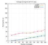
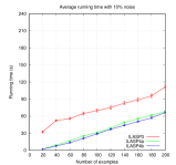
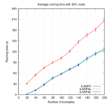
Figure 2: The average computation time of ILASP3, ILASP4a and ILASP4b for the Hamilton learning task, with varying numbers of examples, with 5, 10 and 20% noise.

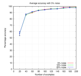
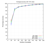
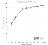
Figure 3: The average accuracies of ILASP3, ILASP4a and ILASP4b for the Hamilton learning task, with varying numbers of examples, with 5, 10 and 20% noise.

For $n\mathchar 61\relax 20,40,\ldots,200$, $n$ random graphs of size one to four were generated, half of which were Hamiltonian. The graphs were labelled as either positive or negative, where positive indicates that the graph is Hamiltonian. Three sets of experiments were run, evaluating each ILASP algorithm with 5%, 10% and 20% of the examples being labelled incorrectly. In each experiment, an equal number of Hamiltonian graphs and non-Hamiltonian graphs were randomly generated and 5%, 10% or 20% of the examples were chosen at random to be labelled incorrectly. This set of examples were labelled as positive (resp. negative) if the graph was not (resp. was) Hamiltonian. The remaining examples were labelled correctly (positive if the graph was Hamiltonian; negative if the graph was not Hamiltonian). Figures 2 and 3 show the average running time and accuracy (respectively) of each ILASP version with up to 200 example graphs. Each experiment was repeated 50 times (with different randomly generated examples). In each case, the accuracy was tested by generating a further 1,000 graphs and using the learned hypothesis to classify the graphs as either Hamiltonian or non-Hamiltonian.

The experiments show that each of the three conflict-driven ILASP algorithms (ILASP3, ILASP4a and ILASP4b) achieve the same accuracy on average (this is to be expected, as each system is guaranteed to find an optimal solution of any task). They each achieve a high accuracy (of well over 90%), even with 20% of the examples labelled incorrectly. A larger percentage of noise means that ILASP requires a larger number of examples to achieve a high accuracy. This is to be expected, as with few examples, the hypothesis is more likely to “overfit” to the noise, or pay the penalty of some non-noisy examples. With large numbers of examples, it is more likely that ignoring some non-noisy examples would mean not covering others, and thus paying a larger penalty. The computation time of each algorithm rises in all three graphs as the number of examples increases. This is because larger numbers of examples are likely to require larger numbers of iterations of the CDILP approach (for each ILASP algorithm). Similarly, more noise is also likely to mean a larger number of iterations. The experiments also show that on average, both ILASP4 approaches perform around the same, with ILASP4b being marginally better than ILASP4a. Both ILASP4 approaches perform significantly better than ILASP3. Note that the results reported for ILASP3 on this experiment are significantly better than those reported in [Law et al. (2018b)]. This is due to improvements to the overall ILASP implementation (shared by ILASP3 and ILASP4).

The effect of constraint propagation.

The final experiment in this section evaluates the benefit of using constraint propagation on noisy learning tasks. The idea of constraint propagation is that although it itself takes additional time, it may decrease the number of iterations of the conflict-driven algorithms, meaning that the overall running time is reduced. Figure 4 shows the difference in running times between ILASP4a with and without constraint propagation enabled on a repeat of the Hamilton 20% noise experiment. Constraint propagation makes a huge difference to the running times demonstrating that this feature of CDILP is a crucial factor in ILASP’s scalability over large numbers of noisy examples.

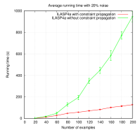
Figure 4: The average running times of ILASP4a with and without constraint propagation enabled for the Hamilton learning task with 20% noise.

6 Related Work

Learning under the answer set semantics.

Traditional approaches to learning under the answer set semantics were broadly split into two categories: brave learners (e.g. [Sakama and Inoue (2009), Ray (2009), Corapi et al. (2011), Katzouris et al. (2015), Kazmi et al. (2017)]), which aimed to explain a set of (atomic) examples in at least one answer set of the learned program; and cautious learners (e.g. [Inoue and Kudoh (1997), Seitzer et al. (2000), Sakama (2000), Sakama and Inoue (2009)]), which aimed to explain a set of (atomic) examples in every answer set of the learned program. In general, it is not possible to distinguish between two ASP programs (even if they are not strongly equivalent) using either brave or cautious reasoning alone [Law et al. (2018a)], meaning that some programs cannot be learned with either brave or cautious induction; for example, no brave induction system is capable of learning constraints – roughly speaking, this is because examples in brave induction only say what should be (in) an answer set, so can only incentivise learning programs with new or modified answer sets (compared to the background knowledge on its own), whereas constraints only rule out answer sets. ILASP [Law et al. (2014)] was the first system capable of combining brave and cautious reasoning, and (resources permitting) can learn any ASP program up to strong equivalence in ASP [Law et al. (2018a)].

FastLAS [Law et al. (2020)] is a recent ILP system that solves a restricted version of ILASP’s learning task. Unlike ILASP, it does not enumerate the hypothesis space in full, meaning that it can scale to solve tasks with much larger hypothesis spaces than ILASP. Although FastLAS has recently been extended [Law et al. (2021)], the restrictions on the extended version still mean that FastLAS is currently incapable of learning recursive definitions, performing predicate invention, or of learning weak constraints. Compared to ILASP, these are major restrictions, and work to lift them is ongoing.

Conflict-driven solvers.

ILASP’s CDILP approach was partially inspired by conflict-driven SAT [Lynce and Marques-Silva (2003)] and ASP [Gebser et al. (2007), Gebser et al. (2011), Alviano et al. (2013)] solvers, which generate nogoods or learned constraints (where the term learned should not be confused with the notion of learning in this paper) throughout their execution. These nogoods/learned constraints are essentially reasons why a particular search branch has failed, and allow the solver to rule out any further candidate solutions which fail for the same reason. The coverage formulas in ILASP perform the same function. They are a reason why the most recent hypothesis is not a solution (or, in the case of noisy learning tasks, not as good a solution as it was previously thought to be) and allow ILASP to rule out (or, in the case of noisy learning tasks, penalise) any hypothesis that is not accepted by the coverage formula.

It should be noted that although ILASP3 and ILASP4 are the closest linked ILASP systems to these conflict-driven solvers, earlier ILASP systems are also partially conflict-driven. ILASP2 [Law et al. (2015)] uses a notion of a violating reason to explain why a particular negative example is not covered. A violating reason is an accepting answer set of that example (w.r.t. $B\cup H$). Once a violating reason has been found, not only the current hypothesis, but any hypothesis which shares this violating reason is ruled out. ILASP2i [Law et al. (2016)] collects a set of relevant examples – a set of examples which were not covered by previous hypotheses – which must be covered by any future hypothesis. However, these older ILASP systems do not extract coverage formulas from the violating reasons/relevant examples, and use an expensive meta-level ASP representation which grows rapidly as the number of violating reasons/relevant examples increases. They also do not have any notion of constraint propagation, which is crucial for efficient solving of noisy learning tasks.

Incremental approaches to ILP.

Some older ILP systems, such as ALEPH [Srinivasan (2001)], Progol [Muggleton (1995)] and HAIL [Ray et al. (2003)], incrementally consider each positive example in turn, employing a cover loop. The idea behind a cover loop is that the algorithm starts with an empty hypothesis $H$, and in each iteration adds new rules to $H$ such that a single positive example $e$ is covered, and none of the negative examples are covered. Unfortunately, cover loops do not work in a non-monotonic setting because the examples covered in one iteration can be “uncovered” by a later iteration. Worse still, the wrong choice of hypothesis in an early iteration can make another positive example impossible to cover in a later iteration. For this reason, most ILP systems under the answer set semantics (including ILASP1 and ILASP2) tend to be batch learners, which consider all examples at once. The CDILP approach in this paper does not attempt to learn a hypothesis incrementally (the hypothesis search starts from scratch in each iteration), but instead builds the set of coverage constraints incrementally. This allows ILASP to avoid the problems of cover loop approaches in a non-monotonic setting, while still overcoming the scalability issues associated with batch learners.

There are two other incremental approaches to ILP under the answer set semantics. ILED [Katzouris et al. (2015)], is an incremental version of the XHAIL algorithm, which is specifically targeted at learning Event Calculus theories. ILED’s examples are split into windows, and ILED incrementally computes a hypothesis through theory revision [Wrobel (1996)] to cover the examples. In an arbitrary iteration, ILED revises the previous hypothesis $H$ (which is guaranteed to cover the first $n$ examples), to ensure that it covers the first $n\mathchar 43\relax 1$ examples. As the final hypothesis is the outcome of the series of revisions, although each revision may have been optimal, ILED may terminate with a sub-optimal inductive solution. In contrast, every version of ILASP will always terminate with an optimal inductive solution if one exists. The other incremental ILP system under the answer set semantics is RASPAL [Athakravi et al. (2013), Athakravi (2015)], which uses an ASPAL-like [Corapi et al. (2011)] approach to iteratively revise a hypothesis until it is an optimal inductive solution of a task. RASPAL’s incremental approach is successful as it often only needs to consider small parts of the hypothesis space, rather than the full hypothesis space. Unlike ILED and ILASP, however, RASPAL considers the full set of examples when searching for a hypothesis.

Popper [Cropper and Morel (2021)] is a recent approach to learning definite programs. It is closely related to CDILP as it also uses an iterative approach where the current hypothesis (if it is not a solution) is used to constrain the future search. However, unlike ILASP, Popper does not extract a coverage formula from the current hypothesis and counterexample, but instead uses the hypothesis itself as a constraint; for example, ruling out any hypothesis that theta-subsumes the current hypothesis. Popper’s approach has the advantage that, unlike ILASP, it does not need to enumerate the hypothesis space in full; however, compared to ILASP it is very limited, and does not support negation as failure, choice rules, disjunction, hard or weak constraints, non-observational predicate learning, predicate invention or learning from noisy examples. It is unclear whether the approach of Popper could be extended to overcome these limitations.

ILP approaches to noise.

Most ILP systems have been designed for the task of learning from example atoms. In order to search for best hypotheses, such systems normally use a scoring function, defined in terms of the coverage of the examples and the length of the hypothesis (e.g. ALEPH [Srinivasan (2001)], Progol [Muggleton (1995)], and the implementation of XHAIL [Bragaglia and Ray (2014)]). When examples are noisy, this scoring function is sometimes combined with a notion of maximum threshold, and the search is not for an optimal solution that minimises the number of uncovered examples, but for a hypothesis that does not fail to cover more than a defined maximum threshold number of examples (e.g. [Srinivasan (2001), Oblak and Bratko (2010), Athakravi et al. (2013)]). In this way, once an acceptable hypothesis (i.e. a hypothesis that covers a sufficient number of examples) is computed the system does not search for a better one. As such, the computational task is simpler, and therefore the time needed to compute a hypothesis is shorter, but the learned hypothesis is not optimal. Furthermore, to guess the “correct” maximum threshold requires some idea of how much noise there is in the given set of examples. For instance, one of the inputs to the HYPER/N [Oblak and Bratko (2010)] system is the proportion of noise in the examples. When the proportion of noise is unknown, too small a threshold could result in the learning task being unsatisfiable, or in learning a hypothesis that overfits the data. On the other hand, too high a threshold could result in poor hypothesis accuracy, as the hypothesis may not cover many of the examples. The $ILP_{LAS}^{noise}$ framework addresses the problem of computing optimal solutions and in doing so does not require any knowledge a priori of the level of noise in the data.

Another difference when compared to many ILP approaches that support noise is that $\textit{ILP}_{\textit{\scriptsize LAS}}^{\textit{ \scriptsize noise}}$ examples contain partial interpretations. In this paper, we do not consider penalising individual atoms within these partial interpretations. This is somewhat similar to what traditional ILP approaches do (it is only the notion of examples that is different in the two approaches). In fact, while penalising individual atoms within partial interpretations would certainly be an interesting avenue for future work, this could be seen as analogous to penalising the arguments of atomic examples in traditional ILP approaches [Law (2018)].

XHAIL is a brave induction system that avoids the need to enumerate the entire hypothesis space. XHAIL has three phases: abduction, deduction and induction. In the first phase, XHAIL uses abduction to find a minimal subset of some specified ground atoms. These atoms, or a generalisation of them, will appear in the head of some rule in the hypothesis. The deduction phase determines the set of ground literals which could be added to the body of the rules in the hypothesis. The set of ground rules constructed from these head and body literals is called a kernel set. The final induction phase is used to find a hypothesis which is a generalisation of a subset of the kernel set that proves the examples. The public implementation of XHAIL [Bragaglia and Ray (2014)] has been extended to handle noise by setting penalties for the examples similarly to $\textit{ILP}_{\textit{\scriptsize LAS}}^{\textit{ \scriptsize noise}}$. However, as shown in Example 7 XHAIL is not guaranteed to find an optimal inductive solution of a task.

Example 7

Consider the following noisy task, in the XHAIL input format:

p(X) :- q(X, 1), q(X, 2).
p(X) :- r(X).
s(a).   s(b).   s2(b).
t(1).   t(2).
#modeh r(+s).
#modeh q(+s2, +t).
#example not p(a)=50.
#example p(b)=100.

This corresponds to a hypothesis space that contains two facts $F_{1}$ = $\mathtt{r(X)}$, $F_{2}$ = $\mathtt{q(X,Y)}$ (in XHAIL, these facts are implicitly “typed”, so the first fact, for example, can be thought of as the rule $\mathtt{r(X)\texttt{:- }s(X)}$). The two examples have penalties 50 and 100 respectively. There are four possible hypotheses: $\emptyset$, $F_{1}$, $F_{2}$ and $F_{1}\cup F_{2}$, with scores 100, 51, 1 and 52 respectively. XHAIL terminates and returns $F_{1}$, which is a suboptimal hypothesis.

The issue is with the first step. The system finds the smallest abductive solution, $\{\mbox{$\mathtt{r(b)}$}\}$ and as there are no body declarations in the task, the kernel set contains only one rule: $\mathtt{r(b)\texttt{:- }s(b)\texttt{.}}$ XHAIL then attempts to generalise to a first order hypothesis that covers the examples. There are two hypotheses which are subsets of a generalisation of $\mathtt{r(b)}$ ($F_{1}$ and $\emptyset$); as $F_{1}$ has a lower score than $\emptyset$, XHAIL terminates and returns $F_{1}$. The system does not find the abductive solution $\{\mbox{$\mathtt{q(b,1)}$},\mbox{$\mathtt{q(b,2)}$}\}$, which is larger than $\{\mbox{$\mathtt{r(b)}$}\}$ and is therefore not chosen, even though it would eventually lead to a better solution than $\{\mbox{$\mathtt{r(b)}$}\}$.

It should be noted that XHAIL does have an iterative deepening feature for exploring non-minimal abductive solutions, but in this case using this option XHAIL still returns $F_{1}$, even though $F_{2}$ is a more optimal hypothesis. Even when iterative deepening is enabled, XHAIL only considers non-minimal abductive solutions if the minimal abductive solutions do not lead to any non-empty inductive solutions.

In comparison to ILASP, in some problem domains, XHAIL is more scalable as it does not start by enumerating the hypothesis space in full. On the other hand, as shown by Example 7, XHAIL is not guaranteed to find the optimal hypothesis, whereas ILASP is. ILASP also solves $ILP_{LAS}^{noise}$ tasks, whereas XHAIL solves brave induction tasks, which means that due to the generality results in [Law et al. (2018a)] ILASP is capable of learning programs which are out of reach for XHAIL no matter what examples are given.

Inspire [Kazmi et al. (2017)] is an ILP system based on XHAIL, but with some modifications to aid scalability. The main modification is that some rules are “pruned” from the kernel set before XHAIL’s inductive phase. Both XHAIL and Inspire use a meta-level ASP program to perform the inductive phase, and the ground kernel set is generalised into a first order kernel set (using the mode declarations to determine which arguments of which predicates should become variables). Inspire prunes rules which have fewer than $Pr$ instances in the ground kernel set (where $Pr$ is a parameter of Inspire). The intuition is that if a rule is necessary to cover many examples then it is likely to have many ground instances in the kernel. Clearly this is an approximation, so Inspire is not guaranteed to find the optimal hypothesis in the inductive phase. In fact, as XHAIL is not guaranteed to find the optimal inductive solution of the task (as it may pick the “wrong” abductive solution), this means that Inspire may be even further from the optimal. The evaluation in [Law et al. (2018b)] demonstrates that on a real dataset, Inspire’s approximation leads to lower quality solutions (in terms of the $F_{1}$ score on a test set) than the optimal solutions found by ILASP.

7 Conclusion

This paper has presented the Conflict-driven Inductive Logic Programming (CDILP) approach. While the four phases of the CDILP approach are clearly defined at an abstract level, there is a large range of algorithms that could be used for the conflict analysis phase. This paper has presented two (extreme) approaches to conflict analysis: the first (used by the ILASP3 system) extracts as much as possible from a counterexample, computing a coverage formula which is accepted by a hypothesis if and only if the hypothesis covers the counterexample; the second (used by the ILASP4 system) extracts much less information from the example and essentially computes an explanation as to why the most recent hypothesis does not cover the counterexample. A third (middle ground) approach is also presented. Our evaluation shows that the selection of conflict analysis approach is crucial to the performance of the system and that although the second and third approaches used by ILASP4 may result in more iterations of the CDILP process than in ILASP3, because each iteration tends to be much shorter, both versions of ILASP4 can significantly outperform ILASP3, especially for a particular type of non-categorical learning task.

The evaluation has demonstrated that the CDILP approach is robust to high proportions of noisy examples in a learning task, and that the constraint propagation phase of CDILP is crucial to achieving this robustness. Constraint propagation allows ILASP to essentially “boost” the penalty associated with ignoring a coverage constraint, by expressing that not only the counterexample associated with the coverage constraint will be left uncovered, but also every example to which the constraint has been propagated.

There is still much scope for improvement, and future work on ILASP will include developing new (possibly domain-dependent) approaches to conflict analysis. The new PyLASP feature of ILASP4 also allows users to potentially implement customised approaches to conflict analysis, by injecting a Python implementation of their conflict analysis method into ILASP.

Another avenue of future work is to develop a version of ILASP that does not rely on computing the hypothesis space before beginning the CDILP process. The FastLAS [Law et al. (2020), Law et al. (2021)] systems solve a restricted $ILP_{LAS}^{noise}$ task and are able to use the examples to compute a small subset of the hypothesis space that is guaranteed to contain at least one optimal solution. For this reason, FastLAS has been shown to be far more scalable than ILASP w.r.t. the size of the hypothesis space. However, FastLAS is far less general than ILASP, reducing its applicability. In future work, we aim to unify the two lines of research and produce a (conflict driven) version of ILASP that uses techniques based on FastLAS to avoid needing to compute the entire hypothesis space.

Appendix A: Conflict-driven Learning of Weak Constraints

In addition to the rules considered in the paper, ILASP is able to learn weak constraints [Law et al. (2015)]. This enables ILASP to perform a kind of preference learning. For simplicity, we omitted details of weak constraint learning from the main paper. In this section, we extend the concepts in the paper to show how ILASP’s new CDILP approach also extends to weak constraint learning.

Appendix A.1: Extra Background Material

Unlike hard constraints in ASP, weak constraints do not affect what is, or is not, an answer set of a program $P$. Hence the above definitions also apply to programs with weak constraints. Weak constraints create an ordering over $AS(P)$ specifying which answer sets are “better” than others. A weak constraint is of the form $\mathtt{:\sim b_{1},\ldots,b_{n},\texttt{not }c_{1},\ldots,\texttt{not }c_{m}\texttt{.}[w@l,t_{1},\ldots,t_{k}]}$ where $\mathtt{b_{1},\ldots,b_{n},c_{1},\ldots,c_{m}}$ are atoms, $\mathtt{w}$ and $\mathtt{l}$ are terms specifying the weight and the level, and $\mathtt{t_{1},\ldots,t_{k}}$ are terms ($\mathtt{[w@l,t_{1},\ldots,t_{k}]}$ is called the tail of the weak constraint). At each priority level $\mathtt{l}$, the aim is to discard any answer set which does not minimise the sum of the weights of the ground weak constraints (with level $\mathtt{l}$) whose bodies are true. The higher levels are minimised first. Terms specify which ground weak constraints should be considered unique. For any program $P$ and $A\in AS(P)$, $\textit{weak}(P,A)$ is the set of tuples $\mathtt{(w,l,t_{1},\ldots,t_{k})}$ for which there is some $\mathtt{:\sim b_{1},\ldots,b_{n},\texttt{not }c_{1},\ldots,}$ $\mathtt{\texttt{not }c_{m}\texttt{.}[w@l,t_{1},\ldots,t_{k}]}$ in the grounding of $P$ such that $A$ satisfies $\mathtt{b_{1},\ldots,b_{n},}$ $\mathtt{\texttt{not }c_{1},\ldots,\texttt{not }c_{m}}$.

In this section, the term ASP program is used to mean a program consisting of a finite set of disjunctive rules and weak constraints. The semantics of weak constraints [ASPCORE2] are defined as follows. For each level $l$, $P^{l}_{A}\mathchar 61\relax\sum_{(w,l,t_{1},\ldots,t_{k})\in\textit{\scriptsize weak}(P,A)}w$. For $A_{1},A_{2}\in AS(P)$, $A_{1}$ dominates $A_{2}$ (written $A_{1}\succ_{P}A_{2}$) iff $\exists l$ such that $P^{l}_{A_{1}}\mathchar 60\relax P^{l}_{A_{2}}$ and $\forall m\mathchar 62\relax l,P^{m}_{A_{1}}\mathchar 61\relax P^{m}_{A_{2}}$. An answer set $A\!\in\!AS(P)$ is optimal if it is not dominated by any $A_{2}\!\in\!AS(P)$.

This paper uses the following notation to describe the preference relationship between a pair of answer sets $A_{1}$ and $A_{2}$, using six binary comparison operators $\{\mathchar 60\relax,\mathchar 62\relax,\leq,\geq,\mathchar 61\relax,\neq\}$.

• $A_{1}\mathchar 60\relax_{P}A_{2}$ iff $A_{1}\succ_{P}A_{2}$ (i.e. iff $A_{1}$ dominates $A_{2}$);

• $A_{1}\mathchar 62\relax_{P}A_{2}$ iff $A_{2}\succ_{P}A_{1}$ (i.e. iff $A_{2}$ dominates $A_{1}$);

• $A_{1}\leq_{P}A_{2}$ iff $A_{2}\not\succ_{P}A_{1}$ (i.e. iff $A_{2}$ does not dominate $A_{1}$);

• $A_{1}\geq_{P}A_{2}$ iff $A_{1}\not\succ_{P}A_{2}$ (i.e. iff $A_{1}$ does not dominate $A_{2}$);

• $A_{1}\mathchar 61\relax_{P}A_{2}$ iff $A_{1}\not\succ_{P}A_{2}$ and $A_{2}\not\succ_{P}A_{1}$ (i.e. iff neither $A_{1}$ nor $A_{2}$ dominates the other);

• $A_{1}\neq_{P}A_{2}$ iff $A_{1}\succ_{P}A_{2}$ or $A_{2}\succ_{P}A_{1}$ (i.e. iff either $A_{1}$ or $A_{2}$ dominates the other).

Let $WC$ be a set of weak constraints. The weak constraints in $WC$ are independent if there are no two weak constraints $W_{1}$ and $W_{2}$ in $WC$ with ground instances $W_{1}^{g}$ and $W_{2}^{g}$ such that the tail of $W_{1}^{g}$ is equal to the tail of $W_{2}^{g}$. In this paper, we only consider programs whose weak constraints are independent.

Ordering Examples.

Positive and negative examples can be used to learn any ASP program consisting of normal rules, choice rules and hard constraints. As positive and negative examples can only express what should or should not be an answer set of the learned program, they cannot be used to learn weak constraints, which do not affect what is or is not an answer set. Weak constraints create a preference ordering over the answer sets of a program, so in order to learn them we need to give examples of this preference ordering – i.e. examples of which answer sets should be preferred to which other answer sets. These ordering examples come in two forms: brave orderings, which express that at least one pair of accepting answer sets for a pair of positive examples is ordered in a particular way; and cautious orderings, which express that every such pair of answer sets should be ordered in that way.

A context-dependent ordering example (CDOE) $o$ is a tuple $\langle e^{1},e^{2},\prec\rangle$, where $e^{1}$ and $e^{2}$ are CDPIs and $\prec$ is a binary comparison operator ($\mathchar 60\relax$, $\mathchar 62\relax$, $\mathchar 61\relax$, $\leq$, $\geq$ or $\neq$). A pair of interpretations $\langle I_{1},I_{2}\rangle$ is said to be an accepting pair of answer sets of $o$ w.r.t. a program $P$ if all of the following conditions hold: (i) $I_{1}\in\textit{AAS}(e^{1},P)$; (ii) $I_{2}\in\textit{AAS}(e^{2},P)$; and (iii) $I_{1}\prec_{P}I_{2}$. A program $P$ is said to bravely respect $o$ if there is at least one accepting pair of answer sets of $o$ w.r.t. $P$. $P$ is said to cautiously respect $o$ if there is no accepting pair of answer sets of $\langle e^{1},e^{2},\prec^{\mathchar 45\relax 1}\rangle$ w.r.t. $P$ (where $\mathchar 60\relax^{\mathchar 45\relax 1}$ is $\geq$, $\mathchar 62\relax^{\mathchar 45\relax 1}$ is $\leq$, $\leq^{\mathchar 45\relax 1}$ is $\mathchar 62\relax$, $\geq^{\mathchar 45\relax 1}$ is $\mathchar 60\relax$, $\mathchar 61\relax^{\mathchar 45\relax 1}$ is $\neq$ and $\neq^{\mathchar 45\relax 1}$ is $\mathchar 61\relax$). In other words, $P$ bravely (resp. cautiously) respects $o$ if at least one (resp. every) pair of answer sets extending the two CDPIs is ordered correctly (w.r.t. $\prec_{P}$).

Learning Task.

Definition 7 formalises the $\textit{ILP}_{\textit{\scriptsize LOAS}}^{\textit{ \scriptsize noise}}$ learning task, which is a generalisation of the $\textit{ILP}_{\textit{\scriptsize LAS}}^{\textit{ \scriptsize noise}}$ task used in the main paper. A rule space $S_{M}$ is a finite set of disjunctive rules and weak constraints, defining the space of programs that are allowed to be learned.

Definition 7

An $\textit{ILP}_{\textit{\scriptsize LOAS}}^{\textit{ \scriptsize noise}}$ task $T$ is a tuple of the form $\langle B,S_{M},\langle E^{\mathchar 43\relax},E^{\mathchar 45\relax},O^{b},O^{c}\rangle\rangle$, where $B$ is an ASP program called the background knowledge, $S_{M}$ is a rule space, $E^{\mathchar 43\relax}$ and $E^{\mathchar 45\relax}$ are (finite) sets of weighted CDPIs and $O^{b}$ and $O^{c}$ are (finite) sets of weighted CDOEs. Given a hypothesis $H\subseteq S_{M}$,

1. $\mathcal{U}(H,T)$ is the set consisting of: (a) all positive examples $e\in E^{\mathchar 43\relax}$ such that $B\cup H$ does not accept $e$; (b) all negative examples $e\in E^{\mathchar 45\relax}$ such that $B\cup H$ accepts $e$; (c) all brave ordering examples $o\in O^{b}$ such that $B\cup H$ does not bravely respect $o$; and (d) all cautious ordering examples $o\in O^{c}$ such that $B\cup H$ does not cautiously respect $o$.

2. the score of $H$, denoted as $\mathcal{S}(H,T)$, is the sum $|H|\mathchar 43\relax\sum_{e\in\mathcal{U}(H,T)}e_{pen}$.

3. $H$ is an inductive solution of $T$ (written $H\in\textit{ILP}_{\textit{\scriptsize LOAS}}^{\textit{ \scriptsize noise}}(T)$) if and only if $\mathcal{S}(H,T)$ is finite.

4. $H$ is an optimal inductive solution of $T$ (written $H\in$ ${}^{*}\textit{ILP}_{\textit{\scriptsize LOAS}}^{\textit{ \scriptsize noise}}(T)$) if and only if $\mathcal{S}(H,T)$ is finite and $\nexists H^{\prime}\subseteq S_{M}$ such that $\mathcal{S}(H,T)\mathchar 62\relax\mathcal{S}(H^{\prime},T)$.

Appendix A.2: Conflict Analysis for CDOE’s

The notion of coverage constraint is slightly extended for ordering examples. This extension is formalised by the following definition.

Definition 8

Let $S_{M}$ be a rule space. A coverage formula over $S_{M}$ takes one of the following forms:

• $R_{id}$, for some $R\in S_{M}$.

• $\Sigma(w_{1}:R_{id}^{1};\ldots;w_{n}:R_{id}^{n})\prec w$, where $R_{1},\ldots,R_{n}\in S_{M}$, $w_{1},\ldots,w_{n},w\in\mathbb{Z}$ and $\prec\in\{\mathchar 60\relax,\mathchar 62\relax,\leq,\geq,\mathchar 61\relax,\neq\}$.

• $\lnot F$, where $F$ is a coverage formula over $S_{M}$.

• $F_{1}\lor\ldots\lor F_{n}$, where $F_{1},\ldots,F_{n}$ are coverage formulas over $S_{M}$.

• $F_{1}\land\ldots\land F_{n}$, where $F_{1},\ldots,F_{n}$ are coverage formulas over $S_{M}$.

The semantics of coverage formulas are defined as follows. Given a hypothesis $H$:

• $R_{id}$ accepts $H$ if and only if $R\in H$.

• $\Sigma(w_{1}:R_{id}^{1};\ldots;w_{n}:R_{id}^{n})\prec w$ accepts $H$ if and only if $\left(\sum\limits_{i\in[1,n],R^{i}\in H}w_{i}\right)\prec w$.

• $\lnot F$ accepts $H$ if and only if $F$ does not accept $H$.

• $F_{1}\lor\ldots\lor F_{n}$ accepts $H$ if and only if $\exists i\in[1,n]$ s.t. $F_{i}$ accepts $H$.

• $F_{1}\land\ldots\land F_{n}$ accepts $H$ if and only if $\forall i\in[1,n]$ s.t. $F_{i}$ accepts $H$.

A coverage constraint is a pair $\langle e,F\rangle$, where $e$ is an example in $E$ and $F$ is a coverage formula, such that for any $H\subseteq S_{M}$, if $e$ is covered then $F$ accepts $H$.

Conflict analysis for brave CDOE’s

Similarly to the iterative approach to conflict analysis for a positive CDPI described in the main paper, ILASP uses an iterative approach to conflict analysis for CDOE’s. Before formalising the method, it is necessary to introduce some additional notation, and a way of computing a coverage formula which can be used to determine whether a pair of interpretations are correctly ordered.

Definition 9

Let $P$ be an ASP program and $I_{1}$ and $I_{2}$ be interpretations. For any integer $l$, the optimisation difference between $I_{1}$ and $I_{2}$ at $l$ with respect to $P$ (denoted $\Delta^{P}_{l}(I_{1},I_{2})$) is equal to $P_{l}^{I_{1}}\mathchar 45\relax P_{l}^{I_{2}}$.

Definition 10

Let $A_{1}$ and $A_{2}$ be a pair of interpretations, $\prec$ be a binary comparison operator and $[l_{1},\ldots,l_{n}]$ be the list of priority levels in $B\cup S_{M}$ (in descending order). For any $l\in[l_{1},\ldots,l_{n}]$, $\omega(T,A_{1},A_{2},l,\prec)$ is the coverage formula $\Sigma(\Delta^{R^{1}}_{l}(A_{1},A_{2}):R_{id}^{1};\ldots;\Delta^{R^{n}}_{l}(A_{1},A_{2}):R_{id}^{n})\prec\Delta^{B}_{l}(A_{1},A_{2})$, where $\{R^{1},\ldots,R^{n}\}\mathchar 61\relax S_{M}$.

Furthermore, $\omega(T,A_{1},A_{2},\prec)$ is the disjunction $F_{1}\lor\ldots\lor F_{n}$, where for each $i\in[1,n]$, $F_{i}\mathchar 61\relax\omega(T,A_{1},A_{2},l_{i},\prec)\land\omega(T,A_{1},A_{2},l_{1},\mathchar 61\relax)\land\ldots\land\omega(T,A_{1},A_{2},l_{i\mathchar 45\relax 1},\mathchar 61\relax)$.

Theorem 7

Let $o$ be a CDOE, $\prec$ be a binary comparison operator and $A_{1}$ and $A_{2}$ be interpretations. A hypothesis $H\subseteq S_{M}$ satisfies $\omega(T,A_{1},A_{2},\prec)$ if and only if $A_{1}\prec_{B\cup H}A_{2}$.

1:procedure iterative_conflict_analysis_CDOE($\langle e_{1},e_{2},\prec\rangle,H,T,\psi$)

2:     $F\mathchar 61\relax\bot$;

3:     while $\exists\langle I_{1},I_{2}\rangle$ s.t. $\exists H\subseteq S_{M}$ s.t. $F$ does not accept $H$, $I_{1}\in\textit{AAS}(e_{1},B\cup H)$, $I_{2}\in\textit{AAS}(e_{2},B\cup H)$ and $I_{1}\prec_{B\cup H}I_{2}$ do

4:         Fix an arbitrary such $\langle I_{1},I_{2}\rangle$

5:         $F\mathchar 61\relax F\lor(\psi(I_{1},I_{2},e_{1},e_{2},\prec,H,T))$;

6:     end while

7:     return $F$;

8:end procedure

Algorithm 3 $\textit{iterative\_conflict\_analysis\_CDOE}(\langle e_{1},e_{2},\prec\rangle,H,T,\psi)$

The iterative_conflict_analysis_CDOE method relies on an extended definition of the three $\psi$’s defined in the main paper. These are formalised by the following definition.

Definition 11

Let $I$ be an interpretation.

• If $I_{1}\in AAS(e_{1},B\cup H)$ and $I_{2}\in AAS(e_{2},B\cup H)$, $\psi_{\alpha}(I_{1},I_{2},e_{1},e_{2},\prec,H,T)\mathchar 61\relax\omega(T,I_{1},I_{2},\prec)$. Otherwise, if $I_{1}$ and $I_{2}$ are both models of $H$, $\psi_{\alpha}(I_{1},I_{2},e_{1},e_{2},\prec,H,T)$ is an arbitrary conjunct of $\mathcal{T}_{2}(I_{1},e_{1},T)$ or $\mathcal{T}_{2}(I_{2},e_{2},T)$ that does not accept $H$. Otherwise, $\psi_{\alpha}(I_{1},I_{2},e_{1},e_{2},\prec,H,T)\mathchar 61\relax\mathcal{T}_{1}(I_{1},e_{1},T)\land\mathcal{T}_{1}(I_{2},e_{2},T)$.

• If $I_{1}\in AAS(e_{1},B\cup H)$ and $I_{2}\in AAS(e_{2},B\cup H)$, $\psi_{\beta}(I_{1},I_{2},e_{1},e_{2},\prec,H,T)\mathchar 61\relax\omega(T,I_{1},I_{2},\prec)$. Otherwise, if $I_{1}$ and $I_{2}$ are both models of $H$, $\psi_{\beta}(I_{1},I_{2},e_{1},e_{2},\prec,H,T)\mathchar 61\relax\mathcal{T}_{2}(I_{1},e_{1},T)\land\mathcal{T}_{2}(I_{2},e_{2},T)$ that does not accept $H$. Otherwise, $\psi_{\beta}(I_{1},I_{2},e_{1},e_{2},\prec,H,T)\mathchar 61\relax\mathcal{T}_{1}(I_{1},e_{1},T)\land\mathcal{T}_{1}(I_{2},e_{2},T)$.

• $\psi_{\gamma}(I_{1},I_{2},e_{1},e_{2},\prec,H,T)\mathchar 61\relax\mathcal{T}(I_{1},e_{1},T)\land\mathcal{T}(I_{2},e_{2},T)\land\omega(T,I_{1},I_{2},\prec)$.

The following two theorems show that, for each of the three $\psi$’s, theiterative_conflict_analysis_CDOE procedure can be used to compute coverage constraints for brave CDOEs. Specifically, they show that the method is guaranteed to terminate and is a valid method for conflict analysis on brave orderings.

Theorem 8

Let $o\mathchar 61\relax\langle e_{1},e_{2},\prec\rangle$ be a CDOE. For each $\psi\in\{\psi_{\alpha},\psi_{\beta},\psi_{\gamma}\}$, the procedure$\textit{iterative\_conflict\_analysis\_CDOE}(o,H,T,\psi)$ is guaranteed to terminate and return a coverage formula $F_{\psi}$. Furthermore, if $o$ is a brave ordering, for each $\psi$ the pair $\langle o,F_{\psi}\rangle$ is a coverage constraint and there is no hypothesis accepted by $F_{\psi}$ that covers $o$.

Conflict analysis for cautious CDOE’s

This section presents two methods of conflict analysis for a cautious CDOE $o$. The first, used by ILASP3, is to call $iterative\_conflict\_analysis\_CDOE(o,H,T,\psi_{\gamma})$. As the result of this is guaranteed to return a coverage formula $F$ that is both necessary and sufficient for $e$ to be accepted, the negation of this formula ($\lnot F$) is guaranteed to be necessary and sufficient for $e$ to not be accepted – i.e. for $e$ to be covered. This result is formalised by Theorem 9.

Theorem 9

Let $o\mathchar 61\relax\langle e_{1},e_{2},\prec\rangle$ be a cautious CDOE (in $O^{c}$). Then$\textit{iterative\_conflict\_analysis\_CDOE}(\langle e_{1},e_{2},\prec^{\mathchar 45\relax 1}\rangle,H,T,\psi_{\gamma})$ is guaranteed to terminate, returning a coverage formula $F$. Furthermore, the pair $\langle o,\lnot F\rangle$ is a coverage constraint and $H$ is not accepted by $\lnot F$.

Similarly to the ILASP4 approach to conflict analysis for negative examples, a coverage constraint can be computed for a cautious ordering example by finding a single pair of interpretations that are ordered incorrectly by the current hypothesis. For a hypothesis to cover the ordering example, it must either not accept one of the two interpretations as an answer set, or it must order them correctly. The coverage formula expressing these three possibilities is formalised and proven to be correct by the following theorem. The computation of this formula is guaranteed to terminate, and the theorem shows that using this formula is a valid method for conflict analysis on cautious ordering examples.

Theorem 10

Let $o\mathchar 61\relax\langle e_{1},e_{2},\prec\rangle$ be a CDOE in $O^{c}$ and $H\subseteq S_{M}$ be a hypothesis that does not cover $o$. There is at least one pair of interpretations $\langle I_{1},I_{2}\rangle$ such that $I_{1}\in\textit{AAS}(e_{1},B\cup H)$, $I_{2}\in\textit{AAS}(e_{2},B\cup H)$ and $I_{1}\prec^{\mathchar 45\relax 1}_{B\cup H}I_{2}$:

1. $\lnot\mathcal{T}(I_{1},e_{1},T)\lor\lnot\mathcal{T}(I_{2},e_{2},T)\lor\omega(T,I_{1},I_{2},\prec)$ does not accept $H$.

2. $\langle o,\lnot\mathcal{T}(I_{1},e_{1},T)\lor\lnot\mathcal{T}(I_{2},e_{2},T)\lor\omega(T,I_{1},I_{2},\prec)\rangle$ is a coverage constraint.

Appendix A.3: Evaluation of CDILP on Preference Learning Tasks

This section presents some extra benchmarks used to evaluate the CDILP approach on weak constraint learning tasks.

Task	$|S_{M}|$	$|E^{\mathchar 43\relax}|$	$|E^{\mathchar 45\relax}|$	$|O^{b}|$	$|O^{c}|$	2i	3	4a	4b
Scheduling (3 day)	180	400	0	110	90	10.14	17.01	3.83	4.25
Scheduling (4 day)	180	400	0	128	72	29.04	36.16	5.17	5.15
Scheduling (5 day)	180	400	0	133	67	53.84	22.63	6.55	6.81
Agent D	244	172	228	390	0	84.51	63.38	38.63	34.99
Journey	117	386	0	200	0	1.35	2.92	1.54	1.66

Table 2: The running times (in seconds) of various ILASP systems on the set of benchmark problems. TO denotes a timeout (where the time limit was 1800s).

The first additional benchmark problem is that of learning scheduling preferences, first presented in [Law et al. (2015)]. In this setting, the goal is to learn an academic’s preferences about interview scheduling, encoded as weak constraints. The tasks in this case are over examples with 3x3, 4x3 and 5x3 timetables, respectively (i.e. three day, four day and five day timetables). In this case, ILASP2i and ILASP3 perform fairly similarly, but both versions of ILASP4 are significantly better either ILASP2i or 3. This task is non-categorical, but in fact as there are only weak constraints in the hypothesis space, for brave orderings ILASP3, ILASP4a and ILASP4b are actually guaranteed to compute the same coverage formula. However, for cautious orderings this is not the case, and the two ILASP4 algorithms will tend to compute shorter formulas than ILASP3 (corresponding to a single pair of answer sets that were ordered incorrectly by the previous hypothesis, rather than all possible pairs of answer sets), although there is still no difference between the two ILASP4 algorithms in this case. This explains the improvement in performance of ILASP4 over ILASP3.

The Agent D learning task is an extension of the Agent benchmarks used in the main paper. In addition to the rules and hard constraints learned in Agent C, weak constraints must be learned to explain why some traces through the grid are preferred to others. This uses positive, negative and brave ordering examples.

The final benchmark is based on a dataset from [Law et al. (2016)], in which the goal is to learn a user’s journey preferences from examples of which journeys the user prefers over other journeys. This task is categorical and contains only weak constraints. For such tasks, ILASP3, ILASP4a and ILASP4b will compute the same coverage formulas in all cases, so there is not much difference between them – minor details of the different implementations cause the ILASP4 approaches to still be slightly faster. All approaches perform similarly to ILASP2i on this task.

References

- Alviano et al. (2013) Alviano, M., Dodaro, C., Faber, W., Leone, N., and Ricca, F. 2013. WASP: A native ASP solver based on constraint learning. In Logic Programming and Nonmonotonic Reasoning, 12th International Conference, LPNMR 2013, Corunna, Spain, September 15-19, 2013. Proceedings. Lecture Notes in Computer Science, vol. 8148. Springer, 54–66.
- Athakravi (2015) Athakravi, D. 2015. Inductive logic programming using bounded hypothesis space. Ph.D. thesis, Imperial College London.
- Athakravi et al. (2013) Athakravi, D., Corapi, D., Broda, K., and Russo, A. 2013. Learning through hypothesis refinement using answer set programming. In Inductive Logic Programming - 23rd International Conference, ILP 2013, Rio de Janeiro, Brazil, August 28-30, 2013, Revised Selected Papers. Lecture Notes in Computer Science, vol. 8812. Springer, 31–46.
- Bragaglia and Ray (2014) Bragaglia, S. and Ray, O. 2014. Nonmonotonic learning in large biological networks. In Inductive Logic Programming - 24th International Conference, ILP 2014, Nancy, France, September 14-16, 2014, Revised Selected Papers. Lecture Notes in Computer Science, vol. 9046. Springer, 33–48.
- Chabierski et al. (2017) Chabierski, P., Russo, A., Law, M., and Broda, K. 2017. Machine comprehension of text using combinatory categorial grammar and answer set programs. In Proceedings of the Thirteenth International Symposium on Commonsense Reasoning, COMMONSENSE 2017, London, UK, November 6-8, 2017. CEUR Workshop Proceedings, vol. 2052. CEUR-WS.
- Corapi et al. (2010) Corapi, D., Russo, A., and Lupu, E. 2010. Inductive logic programming as abductive search. In Technical Communications of the 26th International Conference on Logic Programming, ICLP 2010, July 16-19, 2010, Edinburgh, Scotland, UK. LIPIcs, vol. 7. Schloss Dagstuhl - Leibniz-Zentrum für Informatik, 54–63.
- Corapi et al. (2011) Corapi, D., Russo, A., and Lupu, E. 2011. Inductive logic programming in answer set programming. In Inductive Logic Programming - 21st International Conference, ILP 2011, Windsor Great Park, UK, July 31 - August 3, 2011, Revised Selected Papers. Lecture Notes in Computer Science, vol. 7207. Springer, 91–97.
- Cropper et al. (2020) Cropper, A., Evans, R., and Law, M. 2020. Inductive general game playing. Machine Learning 109, 7, 1393–1434.
- Cropper and Morel (2021) Cropper, A. and Morel, R. 2021. Learning programs by learning from failures. Machine Learning 110, 4, 801–856.
- Cropper and Muggleton (2016) Cropper, A. and Muggleton, S. H. 2016. Metagol system. https://github.com/metagol/metagol.
- Furelos-Blanco et al. (2021) Furelos-Blanco, D., Law, M., Jonsson, A., Broda, K., and Russo, A. 2021. Induction and exploitation of subgoal automata for reinforcement learning. Journal of Artificial Intelligence Research 70, 1031–1116.
- Furelos-Blanco et al. (2020) Furelos-Blanco, D., Law, M., Russo, A., Broda, K., and Jonsson, A. 2020. Induction of subgoal automata for reinforcement learning. In The Thirty-Fourth AAAI Conference on Artificial Intelligence, AAAI 2020, New York, NY, USA, February 7-12, 2020. AAAI Press, 3890–3897.
- Gebser et al. (2011) Gebser, M., Kaminski, R., Kaufmann, B., Ostrowski, M., Schaub, T., and Schneider, M. 2011. Potassco: The Potsdam answer set solving collection. AI Communications 24, 2, 107–124.
- Gebser et al. (2016) Gebser, M., Kaminski, R., Kaufmann, B., Ostrowski, M., Schaub, T., and Wanko, P. 2016. Theory solving made easy with Clingo 5. In Technical Communications of the 32nd International Conference on Logic Programming, ICLP 2016 TCs, October 16-21, 2016, New York City, USA. OASICS, vol. 52. Schloss Dagstuhl - Leibniz-Zentrum für Informatik, 2:1–2:15.
- Gebser et al. (2007) Gebser, M., Kaufmann, B., Neumann, A., and Schaub, T. 2007. Conflict-driven answer set solving. In IJCAI 2007, Proceedings of the 20th International Joint Conference on Artificial Intelligence, Hyderabad, India, January 6-12, 2007. 386.
- Inoue and Kudoh (1997) Inoue, K. and Kudoh, Y. 1997. Learning extended logic programs. In Proceedings of the Fifteenth International Joint Conference on Artificial Intelligence, IJCAI 97, Nagoya, Japan, August 23-29, 1997, 2 Volumes. Morgan Kaufmann, 176–181.
- Kaminski et al. (2019) Kaminski, T., Eiter, T., and Inoue, K. 2019. Meta-interpretive learning using HEX-programs. In Proceedings of the Twenty-Eighth International Joint Conference on Artificial Intelligence, IJCAI 2019, Macao, China, August 10-16, 2019. ijcai.org, 6186–6190.
- Katzouris et al. (2015) Katzouris, N., Artikis, A., and Paliouras, G. 2015. Incremental learning of event definitions with inductive logic programming. Machine Learning 100, 2-3, 555–585.
- Kazmi et al. (2017) Kazmi, M., Schüller, P., and Saygın, Y. 2017. Improving scalability of inductive logic programming via pruning and best-effort optimisation. Expert Systems with Applications 87, 291–303.
- Law (2018) Law, M. 2018. Inductive learning of answer set programs. Ph.D. thesis, Imperial College London.
- Law et al. (2019) Law, M., Russo, A., Bertino, E., Broda, K., and Lobo, J. 2019. Representing and learning grammars in answer set programming. In The Thirty-Third AAAI Conference on Artificial Intelligence, AAAI 2019, Honolulu, Hawaii, USA, January 27 - February 1, 2019. AAAI Press, 2919–2928.
- Law et al. (2020) Law, M., Russo, A., Bertino, E., Broda, K., and Lobo, J. 2020. Fastlas: Scalable inductive logic programming incorporating domain-specific optimisation criteria. In The Thirty-Fourth AAAI Conference on Artificial Intelligence, AAAI 2020, New York, NY, USA, February 7-12, 2020. AAAI Press, 2877–2885.
- Law et al. (2014) Law, M., Russo, A., and Broda, K. 2014. Inductive learning of answer set programs. In Logics in Artificial Intelligence - 14th European Conference, JELIA 2014, Funchal, Madeira, Portugal, September 24-26, 2014. Proceedings. Lecture Notes in Computer Science, vol. 8761. Springer, 311–325.
- Law et al. (2015) Law, M., Russo, A., and Broda, K. 2015. Learning weak constraints in answer set programming. Theory and Practice of Logic Programming 15, 4-5, 511–525.
- Law et al. (2016) Law, M., Russo, A., and Broda, K. 2016. Iterative learning of answer set programs from context dependent examples. Theory and Practice of Logic Programming 16, 5-6, 834–848.
- Law et al. (2018a) Law, M., Russo, A., and Broda, K. 2018a. The complexity and generality of learning answer set programs. Artificial Intelligence 259, 110–146.
- Law et al. (2018b) Law, M., Russo, A., and Broda, K. 2018b. Inductive learning of answer set programs from noisy examples. Advances in Cognitive Systems 7, 57–76.
- Law et al. (2020) Law, M., Russo, A., and Broda, K. 2020. The ILASP system for inductive learning of answer set programs. The Association for Logic Programming Newsletter. https://www.cs.nmsu.edu/ALP/2020/04/the-ilasp-system-for-inductive-learning-of-answer-set-programs/.
- Law et al. (2021) Law, M., Russo, A., Broda, K., and Bertino, E. 2021. Scalable non-observational predicate learning in ASP. In Proceedings of the Thirtieth International Joint Conference on Artificial Intelligence, IJCAI 2021, Virtual Event / Montreal, Canada, 19-27 August 2021. 1936–1943.
- Lynce and Marques-Silva (2003) Lynce, I. and Marques-Silva, J. 2003. The effect of nogood recording in DPLL-CBJ SAT algorithms. In Recent Advances in Constraints. Springer, 144–158.
- Muggleton (1991) Muggleton, S. 1991. Inductive logic programming. New generation computing 8, 4, 295–318.
- Muggleton (1995) Muggleton, S. 1995. Inverse entailment and progol. New generation computing 13, 3-4, 245–286.
- Oblak and Bratko (2010) Oblak, A. and Bratko, I. 2010. Learning from noisy data using a non-covering ILP algorithm. In Inductive Logic Programming - 20th International Conference, ILP 2010, Florence, Italy, June 27-30, 2010. Revised Papers. Lecture Notes in Computer Science, vol. 6489. Springer, 190–197.
- Quinlan (1990) Quinlan, J. R. 1990. Learning logical definitions from relations. Machine learning 5, 3, 239–266.
- Ray (2009) Ray, O. 2009. Nonmonotonic abductive inductive learning. Journal of Applied Logic 7, 3, 329–340.
- Ray et al. (2003) Ray, O., Broda, K., and Russo, A. 2003. Hybrid abductive inductive learning: A generalisation of progol. In Inductive Logic Programming: 13th International Conference, ILP 2003, Szeged, Hungary, September 29-October 1, 2003, Proceedings. Lecture Notes in Computer Science, vol. 2835. Springer, 311–328.
- Sakama (2000) Sakama, C. 2000. Inverse entailment in nonmonotonic logic programs. In Inductive Logic Programming, 10th International Conference, ILP 2000, London, UK, July 24-27, 2000, Proceedings. Lecture Notes in Computer Science, vol. 1866. Springer, 209–224.
- Sakama and Inoue (2009) Sakama, C. and Inoue, K. 2009. Brave induction: a logical framework for learning from incomplete information. Machine Learning 76, 1, 3–35.
- Seitzer et al. (2000) Seitzer, J., Buckley, J. P., and Pan, Y. 2000. Inded: A distributed knowledge-based learning system. IEEE Intelligent Systems and their Applications 15, 5, 38–46.
- Srinivasan (2001) Srinivasan, A. 2001. The aleph manual. https://www.cs.ox.ac.uk/activities/programinduction/Aleph/aleph.html.
- Wrobel (1996) Wrobel, S. 1996. First order theory refinement. Advances in inductive logic programming 32, 14–33.