Metastable Helium Absorptions with 3D Hydrodynamics and
Self-Consistent Photochemistry II:
WASP-107b, Stellar Wind, Radiation Pressure, and Shear Instability

Abstract

This paper presents simulations of the metastable helium ($\mathrm{He}^{*}$) observations of WASP-107b, so far the highest signal-to-noise ratio detection that is confirmed by three different instruments. We employ full 3D hydrodynamics coupled with co-evolving non-equilibrium thermochemistry and ray-tracing radiation, predicting mass loss rates, temperature profiles, and synthetic $\mathrm{He}^{*}$ line profiles and light curves from first principles. We found that a stellar wind stronger than solar is demanded by the observed heavily blueshifted line profile and asymmetric transit light curve. Contrary to previous beliefs, we argue that radiation pressure can be important for Ly$\alpha~{}$observations but not $\mathrm{He}^{*}$. We found WASP-107b is losing mass at a rate of $\dot{M}\simeq 1.0\times 10^{-9}~{}M_{\oplus}~{}\mathrm{yr}^{-1}$. Although $\dot{M}$ varies by $<1~{}\%$ given constant wind and irradiation from the host, shear instabilities still emerge from wind impacts, producing $\sim 10~{}\%$ fluctuations of $\mathrm{He}^{*}$ transit depths over hour-long timescales. The common assumption that $\mathrm{He}^{*}$ transit depth indicates the fluctuation of $\dot{M}$ is problematic. The trailing tail is more susceptible than planet adjacency to the shear instabilities, thus the line profile is more variable in the blue-shifted wing, while the transit light curve is more variable after mid-transit. We stress the synergy between Ly$\alpha~{}$(higher altitudes, lower density) and $\mathrm{He}^{*}$ (lower altitudes, higher density) transit observations, particularly simultaneous ones, yield better understanding of planetary outflows and stellar wind properties.

1 Introduction

The “He i $10830~{}\text{\AA}$ line” or the “metastable helium line” ($\mathrm{He}^{*}$ line for short) transitions between the $2^{3}$S and the upper $2^{3}$P_J ($J=0,1,2$) states are radiatively decoupled from the ground state (for a magnetic dipole transition) and have slow spontaneous decay rates: $A\simeq 1.3\times 10^{-3}~{}\mathrm{s}^{-1}$ (Drake, 1971). The high cosmic abundance of helium, the absence of interstellar absorption and the observability from the ground together enable the $\mathrm{He}^{*}$ lines as a unique probe of atmospheric outflows from exoplanets. The first secure detection of $\mathrm{He}^{*}$ in transmission was made for WASP-107b with the Hubble Space Telescope (Spake et al., 2018). This detection rekindled decade-long interest in this transition (Seager & Sasselov, 2000; Turner et al., 2016; Oklopčić & Hirata, 2018); many more detections around other exoplanets have been made since then (e.g. Allart et al., 2018; Nortmann et al., 2018; Salz et al., 2018; Kirk et al., 2020; Ninan et al., 2020).

There is no surprise that WASP-107b was the first exoplanet to show $\mathrm{He}^{*}$ detection. The host is young ($\sim 600~{}{\rm Myr}$ from gyrochronology) and active (chromospheric activity index $S=0.89$), expected to give out strong high-energy radiation that powers planetary photoevaporative outflow. The host’s spectral type is K6, which is right at the sweet spot of EUV-FUV flux ratio that maximally favors the $\mathrm{He}^{*}$ absorption (Oklopčić 2019; Paper I). The planet is puffy and susceptible to outflows: it has a mass of an icy giant ($0.12~{}M_{\rm Jup}$) but a radius closer to that of Jupiter ($0.94~{}M_{\rm Jup}$). The optical transit depth is $\sim 2.2~{}\%$, while the $\mathrm{He}^{*}$ transit depth is a whopping $\sim 7~{}\%$. The mean density of the planet is only $\sim 0.19~{}\mathrm{g}~{}\mathrm{cm}^{-3}$, which is reminiscent of the anomalously low-density planets ”super-puffs” (e.g. Libby-Roberts et al., 2020; Chachan et al., 2020). Wang & Dai (2019) and Gao & Zhang (2020) proposed that “super-puffs” may appear inflated due to high-altitude dusts or hazes elevated by an outflowing atmosphere; the near-infrared HST observation (Kreidberg et al., 2018) is indeed suggestive of high-altitude condensates partially muting the transmission features. WASP-107b is also dynamically interesting. Dai & Winn (2017) suspected the planet is on a polar orbit due to the lack of repeating spot-crossing events. More recently, a Rossiter-McLaughlin measurement by Rubenzahl, R. et al (in prep) confirmed this suspicion and thus demands a dynamically hot formation and evolution pathway that may involve the non-transiting planet 107c ($P\sim 1100~{}{\rm days}$, $M\sin i\sim 110~{}M_{\oplus}$; Piaulet, C. et al., submitted)

These reasons render WASP-107b a unique and interesting system. The $\mathrm{He}^{*}$ transits of WASP-107b have been observed multiple times (Spake et al., 2018; Allart et al., 2018; Kirk et al., 2020). Its well-resolved line profile exhibits asymmetric shape skewing towards the blue-shifted wing, which suggests a comet-like tail. The line ratio of three different $2^{3}$P_J levels also seems to deviate from the simple quantum degeneracy ratio of 1:3:5 (or 1:8 given that the two latters are not distinguishable). Having been confirmed by different instruments (CARMENES; Keck/NIRSPEC), these features are likely attributed to the morphology and kinematics of planetary outflows, rather than instrumental effects.

The $\mathrm{He}^{*}$ dataset of WASP-107b potentially very revealing and should be analyzed in detail. Two models have been presented in the literature: the 1D isothermal model by Oklopčić & Hirata (2018) assumes the density and velocity profile of a Parker Wind (Parker, 1958). The model has to assume, rather than predict, the mass loss rate and temperature of the outflow. Moreover, 1D models are unable to capture the full orbital dynamics and cannot produce a comet-like tail. The alternative model is the EVaporating Exoplanets code (EVE; see Bourrier et al., 2015; Allart et al., 2018). The lower layer (thermosphere) of this model is also a Parker Wind solution; the upper layer is a Monte-Carlo particle simulations with He particles under the influence of planetary and stellar gravity and radiation pressure. As we will elaborate later in this work, nevertheless, particle-based code may not be appropriate for simulating $\mathrm{He}^{*}$ transits. The authors of EVE acknowledged that the particle-based treatment of radiation pressure accelerates the outflow way too quickly: they had to artificially decrease the stellar spectrum near the $\mathrm{He}^{*}$ lines by a factor of $\sim 50$ to achieve reasonable agreement with the observations of WASP-107b.

In this work, we applied to WASP-107b our model that conducts 3D hydrodynamics, self-consistent thermochemistry, ray-tracing radiative transfer, and especially the processes that populate and destroy $\mathrm{He}^{*}$ (see the first paper in the series, Wang, L. & Dai, F., submitted; Paper I hereafter). Starting from the observed stellar and planetary properties, and making assumptions of the high energy spectral energy distribution (SED) of the host, we can predict the mass loss rate, the temperature profile, the ionization states and the various $\mathrm{He}^{*}$ simulations of WASP-107b. We will also use WASP-107b as a case study to investigate how stellar wind, radiation pressure and shear instability affect planetary outflows and their observability.

This paper is structured as follows: in §2, we will briefly described our model and simulation setup. In §3, we present the fiducial model of WASP-107b that shows remarkable agreement with observation. §4, we perturb the fiducial model in various parameters to investigate §6 summarize the paper and figure out prospective improvements for the future.

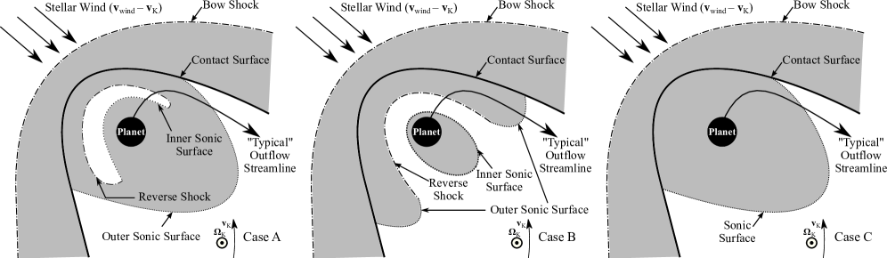
Figure 1: Schematic diagrams (not to scale) of the interactions between a stellar wind and a planetary atmospheric outflow (see also §2.2). In all panels, the host star resides to the left of the diagrams, and the planet’s linear Keplerian velocity points upwards within the paper plane (see the indicators of $\mathbf{v}_{\mathrm{K}}$ and $\mathbf{\Omega}_{\mathrm{K}}$ at the lower-left corner of all panels). Subsonic regions are illustrated by grey shades. Typical streamlines are indicated by thin solid lines with arrow heads. Shock fronts, including the bow shocks and the reverse shock, are indicated by dash-dotted lines. Contact surfaces (contact discontinuities) are shown by heavy solid lines. Dotted lines indicate the sonic critical surfaces. The left panel, marked as Case A, shows a typical case that part of the the planet outflow experiences initial thermally driven acceleration, reverse shock deceleration (due to the stagnation and deflection by the stellar wind), and final acceleration by expansion. Note that the outer sonic surface is connected to the reverse shock, and any streamline crossing the outer sonic surface must go through the reverse shock front. The middle panel presents Case B, which is qualitatively similar to Case A but has different topologies. The right panel presents another typical Case C, which does not have a reverse shock: the planet outflow stays subsonic before the stagnation and deflection, and only become supersonic after it already escapes from the “trap” shaped by the stellar wind.

2 Methods

2.1 Basic Setup

Our numerical simulation suite was described in detail in Paper I. For a brief re-cap, our simulation is carried in 3D with gravity of both the host star and the planet, and the effects of orbital motion including centrifugal and Coriolis forces. Our code computes ray-tracing radiative transfer and non-equilibrium thermochemistry simultaneously with hydrodynamics. For simplicity, we assume circular orbit and that the planet is tidally locked, adopting a co-rotating planet-centric frame. We focus on the upper layer of the atmosphere, including a quasi-isothermal layer assumed to have equilibrium temperature, and an outflowing region irradiated by high-energy photons. The boundary conditions are set so that the observed mass and transit radius of the planet can be reproduced. We describe the high-energy spectral energy distribution (SED) of the host star with 6 characteristic energy bins: (1) $2~{}\mathrm{eV}$ for the near-infrared and optical bands; (2) $7~{}\mathrm{eV}$ for far ultraviolet (FUV) photons (“soft FUV”; note that these photons can ionize $\mathrm{He}^{*}$); (3) $12~{}\mathrm{eV}$ for the Lyman-Werner (“LW”) band FUV photons that photodissociate molecular hydrogen, (4) $20~{}\mathrm{eV}$ for “soft” extreme ultraviolet (“soft EUV”) photons that ionize hydrogen but not helium, (5) $40~{}\mathrm{eV}$ for EUV and soft X-ray (“hard EUV”) photons that ionize helium, and (6) $3~{}\mathrm{keV}$ photons for the X-ray. We make synthetic observations including $\mathrm{He}^{*}$ line profiles and transit light curves in the vicinity of $\mathrm{He}^{*}$ line. To further facilitate comparisons between observation and simulations, we compute summary statistics such as the equivalent widths $\langle W_{\lambda}\rangle\equiv\int\Delta\epsilon(\lambda)~{}\mathrm{d}\lambda$, the radial velocity shift of the absorption peak $\Delta v_{\rm peak}$, and the full-width-half-maximum (FWHM) of the absorption line profile.

Specifically for WASP-107, Anderson et al. (2017) reported a K6 host star with a mass of $M_{*}=0.69~{}M_{\odot}$ and a radius of $R_{*}=0.66~{}R_{\odot}$, and an effective temperature of $T_{*,\mathrm{eff}}=4430~{}\mathrm{K}$. Planet b orbits its host on a near-circular but polar orbit (Dai & Winn, 2017, Piaulet, C. et al, submitted; Rubenzahl, R. et al, submitted). The semi-major axis is $a=0.055~{}\mathrm{AU}$ where the equilibrium temperature is $T_{\mathrm{eq}}=740~{}\mathrm{K}$; the transit light curve indicates a small impact parameter ($b=0.07$ Dai & Winn, 2017). WASP-107b has an optical transiting radius of $R_{\rm p}\simeq 0.94~{}R_{\rm Jup}$ and a mass $M_{\rm p}\simeq 0.12~{}M_{\rm Jup}$.

2.2 Including Stellar Wind and Radiation Pressure

The $\mathrm{He}^{*}$ observables of WASP-107b is highly suggestive of an outflow morphology similar to a comet-like tail, as the reader will find out shortly (§3.1, 3.2). We explore two possible mechanisms that may give rise to the comet-like tail: stellar wind and radiation pressure. For stellar winds, although realistic patterns of stellar winds could be very complicated, we take a very basic approach here. The stellar wind is injected as a hydrodynamic flow in a simulation, with two velocity components in the planet frame: (1) a radial component centered at the host star, and (2) a headwind due to orbital motion of the planet. The first component has the radial wind speed as a parameter; the second one is set to be equivalent to the orbital velocity of the planet.

The regions of interactions between the stellar wind and the planet outflow are illustrated by Figure 1. Depending on whether the velocity already becomes supersonic before being decelerated and deflected by the impinging stellar wind, a fluid element in the planet outflow should go through the sonic critical surface twice (part of streamlines in “Case A” and “Case B”) or once (the complement part of streamlines in Cases A and B, and all streamlines in “Case C”). We note that a streamline in Cases A and B must go through the reverse shock when and only when it crosses the sonic critical surface twice. The first sound crossing occurs at smaller radii (“inner” sonic surface) as the fluid element is accelerated by the thermal pressure gradient. However, as the upwind part is impinged by the stellar wind, the streamline travels through a reverse shock and is decelerated to subsonic. The fluid element then changes its direction, and become deflected to move in the night side. The confinement due to stellar wind then becomes weaker, and the fluid element is allowed to expand like in a de Laval nozzle before eventually becoming supersonic again at a second (“outer”) sonic surface. Other streamlines go through the inner sonic surface only, and never touches the outer sonic surface or the reverse shock front.

Stellar winds impose more stringent Courant-Friedrichs-Lewy conditions: each model takes $\sim 51~{}\mathrm{hr}$ to run on a 40-core, 4-GPU computing node of the Popeye-Simons Computing Cluster. To accelerate the convergence of our simulations, in addition to the “adaptive coarsening” technique in Paper I, we also adopt a two-step scheme of simulation: (1) turn on hydrodynamics, thermochemistry and radiative transfer, run the simulation for $\sim 15~{}\tau_{\mathrm{dyn}}$ until the model almost reaches the quasi-steady state without stellar winds; (2) turn on the stellar wind and continue the simulation for $\gtrsim 200~{}\tau_{\mathrm{dyn}}$ until the final quasi-steady state is reached. The dynamical timescale for a $T\sim 10^{4}~{}\mathrm{K}$ photoevaporative outflow around WASP-107b is estimated as $\tau_{\mathrm{dyn}}\sim 4.8\times 10^{3}~{}\mathrm{s}$:

$$\tau_{\mathrm{dyn}}\sim\dfrac{GM_{\rm p}}{c_{s}^{3}}\sim 1.2\times 10^{3}~{}\mathrm{s}\times\left(\dfrac{M_{p}}{10~{}M_{\oplus}}\right)\left(\dfrac{T}{10^{4}~{}\mathrm{K}}\right)^{-3/2}\ .$$ (1)

To ensure that the simulations are not limited by the spatial resolution of simulation grid, we ran a model with a higher resolution ($N_{\log r}\times N_{\theta}\times N_{\phi}=192\times 192\times 128$) and the results are most identical to that of our standard grid (Figure 3).

Another potentially influential factor is the radiation pressure. We added this effect to our ray-tracing radiative transfer procedures by explicitly computing the momenta deposited by the photons absorbed or scattered. As §5.1 will discuss, the radiative pressure on $\mathrm{He}^{*}$ transitions plays a very minor role on the overall dynamics and $\mathrm{He}^{*}$ observables.

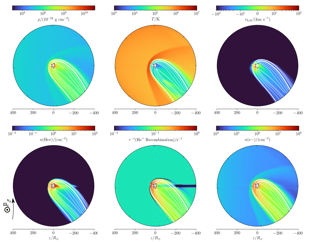
Figure 2: Key hydrodynamics and chemistry profiles of the simulation for WASP-107b (fiducial model 107-0) in the quasi-steady-state, averaged through the last $15~{}\tau_{\mathrm{dyn}}$. Stellar radiation comes from the left of the plot, and the orbital angular velocity $\mathbf{\Omega}_{\mathrm{K}}$ points out of the paper plane; the Keplerian motion of the planet is upwards $\mathbf{v}_{\mathrm{K}}$. White streamlines are separated at the wind base by $\Delta\theta=\pi/16$. Note that only the inner sonic surface is shown (in dashed black curve; see also the Case A in Figure 1). The heavy streamline are the reference lines on which the profiles are plotted in Figure 3).

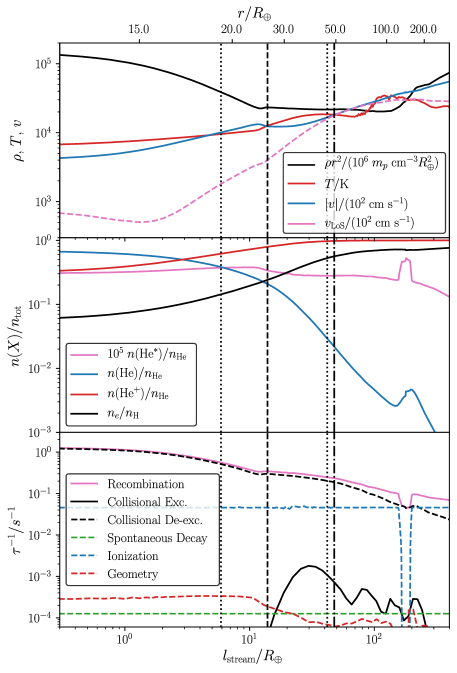
Figure 3: Key quantities of our fiducial model for WASP-107b (Model 107-0), time-averaged over the last $15~{}\tau_{\mathrm{dyn}}$, along the reference streamlines (plotted as the heavy streamline in Figure 2). The top abscissa is the radial coordinate $r$ corresponding to the curve length along the streamline on the bottom abscissa. As explained by §2.2 and the Case A in Figure 1, the fluid elements along this streamline experience two smooth crossings of sonic speed (indicated by vertical dotted lines; note that the right of them is close to the dash-dotted line for the Roche radius) and a reverse shock (indicated by vertical dashed lines) along the streamline.

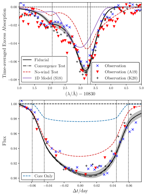
Figure 4: The observed and synthesized line profiles and light curves for the fiducial model of WASP-107b and its corresponding test models. Curves for all models indicate the averages of the spectral profile and light curves over the last $15~{}\tau_{\mathrm{dyn}}$ (note that they are obtained by calculating the profiles for each snapshot before taking the average, not by evaluating the profiles for the time-averaged model). Grey shades around the curves for the fiducial model in both panels express the range of two-times standard deviation ($2\sigma$) over the last $15~{}\tau_{\mathrm{dyn}}$. The observation results in Kirk et al. (2020) are denoted by black “+” and labeled with “Observation (K20)”; those marked with red triangles and “Observation (A19)” presents the results in Allart et al. (2019). The 1D spherical symmetric model in Spake et al. (2018) is included for reference, marked by the magenta curve with label “1D Model (S18)” in the upper panel. For reasonable comparisons, the window function for light curves is taken to be the same as Kirk et al. (2020), i.e. a top-hat function which has unitary value in $(\lambda/\text{\AA})\in[10833.05,10833.48]$ and zero elsewhere (note that the window in Allart et al. (2019) is different, $(\lambda/\text{\AA})\in[10832.80,10833.55]$). Vertical dotted lines in the upper panel shows the centers of the three $\mathrm{He}^{*}$ lines, and mark the start/end of the nominal ingress/egress ($t_{\textsc{{i}}}$ through $t_{\textsc{{iv}}}$) in the lower panel.

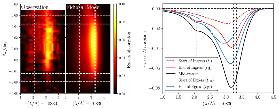
Figure 5: Left panel: Comparison of the excess absorption features, as functions of transit time $\Delta t$ and wavelength $\lambda$, between the observation data (left panel) and the synthesized results (right panel). The simulation used to produce the right panel is the time-averaged fiducial Model 107-0 (averaging is taken in the same way as Figure 4, viz. averaging after the excess absorption map being obtained for each snapshot concerned). Both panels already have the wavelength shifts by orbital motion subtracted. Three vertical dotted lines in each panel indicate the the line centers. Four horizontal dashed lines indicate the starts (ends) of the ingress (egress). Right panel: transmission spectra at different stages of a transit, based on the fiducial Model 107-0.

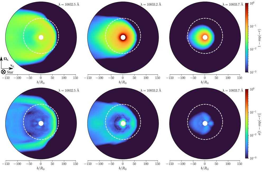
Figure 6: First row: extinction $[1-\exp(-\tau)]$ for Model 107-0 with time-averaging over the last $\sim 15~{}\tau_{\mathrm{dyn}}$ (note that the averaging is computed after the extinction function is calculated for each snapshot concerned) at three representative wavelengths $(\lambda/\text{\AA})\in\{10832.5,10833.2,10833.7\}$ near the $\mathrm{He}^{*}$ transitions. The profiles are measured at mid-transit. Second row presents the root-mean-squared variations of extinction ($\sigma[1-\exp(-\tau)]$). Plotted up to the impact parameter $b=150~{}R_{\oplus}$. The white dashed circles presenting the host star size have $R_{*}\simeq 74.2~{}R_{\oplus}$ and orbit impact parameter $b\simeq 0.07~{}R_{*}$.

Table 1: Properties of the fiducial model for WASP-107b

Item	Value
Simulation domain
Radial range	$10.21~{}R_{\oplus}\leq r\leq\ 400~{}R_{\oplus}$
Latitudinal range	$0\leq\theta\leq\pi$
Azimuthal range	$0\leq\phi\leq\pi$
Resolution $(N_{\log r}\times N_{\theta}\times N_{\phi})$	$144\times 128\times 64$
Planet interior†
$M_{\mathrm{rcb}}$	$38.1~{}M_{\oplus}$
$\langle r_{\mathrm{eff}}\rangle$	$10.6~{}R_{\oplus}$
Radiation flux [photon $\mathrm{cm}~{}^{-2}~{}\mathrm{s}^{-1}$]
$2~{}\mathrm{eV}$ (IR/optical)	$2.1\times 10^{19}$
$7~{}\mathrm{eV}$ (Soft FUV)	$1.2\times 10^{16}$
$12~{}\mathrm{eV}$ (LW)	$3\times 10^{12}$
$20~{}\mathrm{eV}$ (Soft EUV)	$2\times 10^{13}$
$40~{}\mathrm{eV}$ (Hard EUV)	$6\times 10^{13}$
$3~{}\mathrm{keV}$ (X-ray)	$2\times 10^{12}$
Initial abundances [$n_{\mathrm{X}}/n_{\mathrm{H}}$]	Same as Paper I
Dust/PAH properties	Same as Paper I
Stellar wind (at $a=0.055~{}\mathrm{AU}$)
Density	$1.7\times 10^{-19}~{}\mathrm{g}~{}\mathrm{cm}^{-3}$
Temperature	$10^{6}~{}\mathrm{K}$
Radial velocity	$270~{}\mathrm{km}~{}\mathrm{s}^{-3}$
Tangential velocity∗	$106~{}\mathrm{km}~{}\mathrm{s}^{-3}$
Abundances‡ [$n_{\mathrm{X}}/n_{\mathrm{H}}$]
$\mathrm{e}^{-}$	$\simeq 1.1^{**}$
$\mathrm{H}^{+}$	1.0
$\mathrm{He}^{+}$	0.1
$\mathrm{O}^{+}$	$3.2\times 10^{-4}$
$\mathrm{C}^{+}$	$1.4\times 10^{-4}$
$\mathrm{S}^{+}$	$2.8\times 10^{-5}$
$\mathrm{Si}^{+}$	$1.7\times 10^{-6}$

Note. — $\dagger$: Mass and transit radius of the planet core; see also Appendix A of Paper I for details of planet core setups.

$\ddagger$: Because the wind injection has a star-centered geometry, these values are calibrated at the planetary orbit, viz. $a=0.055~{}\mathrm{AU}$.

$*$: Head wind component; same as the Keplerian velocity.

$\ddagger$: Calibrated at the domain boundary of wind injection.

$**$: Electrical neutrality is guaranteed.

3 WASP-107b:
an outflow shaped by stellar winds

3.1 Observation Results

Quantitatively, we directly compare our synthetic observations to $\mathrm{He}^{*}$ line profiles and light curves. The $\mathrm{He}^{*}$ transmission spectrum of WASP-107b is both spectrally and temporally resolved with different spectrographs: NIRSPEC and CARMENES (Spake et al., 2018; Allart et al., 2019; Kirk et al., 2020). We also carried out an independent analysis of the transit observed from NIRSPEC on the Keck telescope on April 6th, 2019 (same as Kirk et al., 2020). Our data reduction is carried out using the procedures described in Zhang, Z. et al. (submitted). $\mathrm{He}^{*}$ transits have been observed by several different instruments and different transit events (Figure 4). Despite the differences in instrumental characteristics and reduction pipelines, previous $\mathrm{He}^{*}$ observations agree with each other on the following features: (1) a non-Keplerian, blueshifted ($\sim 2-3~{}\mathrm{km}~{}\mathrm{s}^{-1}$) line profile; (2) a line ratio that deviates from the 1:3:5 (viz. the quantum degeneracies; apparently 1:8) among three $\mathrm{He}^{*}$ transitions; (3) elongated ingress and egress timescales in $\mathrm{He}^{*}$ transit light curves. Finally, in the temporally resolved observation (Kirk et al., 2020), there is a hint of asymmetry in the outflow morphology that the egress lasts longer than the ingress while the egress is more blueshifted compared to the mid-transit (see also Figure 5).

3.2 Fiducial Model Setup and Necessity of Stellar Winds

As noted in Paper I, consistent 3D hydrodynamic simulations with all physics are not sufficiently fast for a comprehensive exploration of the parameter space using Markov Chain Monte Carlo or even just gradient descent. Instead, we adopt the parameters based on the reported stellar and planetary conditions. The optical and near-infrared fluxes (represented by the $h\nu=2~{}\mathrm{eV}$ bin) simply accord with the host star radius and effective temperature. The high energy SED of the host star is much more uncertain. Guided by the results in our Paper I, i.e. how various high-energy radiation bins affect the atmospheric outflow and $\mathrm{He}^{*}$ observables, we hand-tuned the high-energy SED until reasonable agreement with the observations. The resulting high-energy SED is fairly typical or slightly more active than a K5 star (Gudel, 1992; France et al., 2016; Youngblood et al., 2016; Loyd et al., 2016; Youngblood et al., 2017; Oklopčić, 2019), but we also note that WASP-107b has a relatively short rotation period of 17 days, and the $\sim 600~{}{\rm Myr}$ host star has a strong chromospheric S index (0.89) (Dai & Winn, 2017).

In addition to tuning the high-energy SED, we found it crucial to include stellar wind components in our simulations to adequately reproduce the existing $\mathrm{He}^{*}$ observations. We first run a series of no-wind model as we did in Paper I for WASP-69b. The resultant outflow is largely spherically isotropic, without prominent comet-like tail. Figure 4 presents the $\mathrm{He}^{*}$ line profile and light curves produced in the no-wind fiducial model (other parameters are the same as those in Table 1). The overall equivalent width of the line profile is weaker ($\langle W_{\lambda}\rangle\simeq(7.6\pm 0.2)~{}\text{\AA}$ in the fiducial model, but $\langle W_{\lambda}\rangle\simeq 5.0~{}\text{\AA}$ in the no-wind model). More importantly, the line profile does not have a stronger blueshifted wing, which has been validated by several different instruments.The impinging stellar wind stagnates the outflow flowing towards the host star (i.e. the redshifted wing), pushing the outflow to the night-side (the blueshifted wing). The transit light curve in the no-wind model is also much more symmetric compared due to the lack of comet-like tail trailing behind the planet. In short, a no-wind model struggles, if ever possible, to reproduce the various $\mathrm{He}^{*}$ observations of WASP-107b. On the other hand, the windy model successfully reproduced observed $\mathrm{He}^{*}$ line profiles and light curves. We now examine the windy model in detail.

3.3 Fiducial Model Results

Figure 2 presents the simulation results of our fiducial model, with a stellar wind modulating the outflow morphology. Each panel centers at the planet’s frame; the host star is located to the left of the this plot, and the stellar wind impinges on the photoevaporative outflow at an angle given by the ratio between the radial velocity component and the headwind (orbital) component. A bow shock of Mach number $\sim 2.0$ forms above the day-side of the planet, heating the downstream flow to $T\sim 4\times 10^{6}~{}\mathrm{K}$ (second panel of Figure 2). As shown by the streamlines, the photoevaporative outflow from the planet is stalled at the day-side and directed by stellar wind to the night-side, forming a prominent tail trailing the planet’s orbital motion.

Along the thick streamline in Figure 2 (which qualitatively resembles the “typical” streamline in Figure 1), we plot the spatial variation of key hydrodynamic and thermochemical quantities both as a function of radius from the planet core and the arc length along the streamline in Figure 3. Looking at the outflow velocity first, a fluid element traveling on the streamline may experience multiple sound crossings, as is shown by the Case A in Figure 1 (see also §2.2). We note that this effect is strongest at the upwind side where outflow is impinged by stellar wind; it is much weaker elsewhere and the reverse shock may no longer exist. The lower panel of Figure 3 indicates that the population of $\mathrm{He}^{*}$ is determined primarily by the equilibrium between recombination excitation and collisional de-excitation at smaller radii. At larger radii ($\gtrsim 10^{2}~{}R_{\oplus}$), photoionization by soft FUV photons starts to take over. This is very similar to our results in Paper I for WASP-69b.

The middle panel of Figure 3 shows another interesting feature. When the streamline crosses the the planet’s shadow, photoionization due to soft FUV from the host star vanishes. However, recombination excitation continues in the shadow of the planet and thus creates a local bump of higher $\mathrm{He}^{*}$ abundances. We call this effect the “shadow tail”. Such a feature is difficult to observe in transits as it always hides in the planet’s shadow. If one is ever able to resolve this photoevaporative outflow, one may see the shadow tail emitting more strongly in $\mathrm{He}^{*}$ compared to other parts of the outflow. Such a “two-tail” morphology is remarkably similar to the dust and ion tails of a comets, although with different underlying physics.

Figure 6 offers a transverse view of the outflow, taken from the perspective of an observer looking into the host star (outlined as the white dashed-line) during a transit. The planet is moving towards the right-hand-side, and is instantaneously close to the center of the host star. These plots illustrate the spatial distribution of extinction at three characteristic wavelengths of the $\mathrm{He}^{*}$ transition. At the bluer wavelength $\lambda=10832.5~{}\text{\AA}$, which falls into the “valley” between the $J=0$ transition and two blended $J=1,2$ transitions, the extinction is dominated by blueshifted materials in the tail trailing behind the planet. On the red wing $\lambda=10833.7~{}\text{\AA}$, the tail is much less relevant, and the extinction are generated by materials much closer to the planet. Again, this is attributed to the kinematics and morphology: the planetary outflow is impinged by the stellar wind, and the outflow on the day-side or the headwind direction is stagnated.

Finally, we remind the reader that due to its large aperture, Keck/NIRSPEC is able to resolve the $\mathrm{He}^{*}$ both spectrally and temporally. Figure 5 presents the observed and simulated variation of $\mathrm{He}^{*}$ absorption in time and wavelength space together as a heatmap. The vertical dotted lines are the rest-frame wavelengths of three $\mathrm{He}^{*}$ transitions, the horizontal dashed lines are the expected $t_{\textsc{{i}}}$ to $t_{\textsc{{iv}}}$ (starts/ends of the ingress/egress) of the planet’s transit. Our simulation with stellar winds successfully reproduces the key feature: since most of the $\mathrm{He}^{*}$ is produced by the comet-like tail trailing the planet (Figure 6), the strongest absorption occurs after mid-transit, while the pre-ingress absorption is much weaker than the post-egress one. This feature is also manifested by the asymmetry in the transit light curve (Figure 4). The outflow morphology loses spherical symmetry; the part ahead of the planet and behind the planet are both blueshifted. As a result, the $\mathrm{He}^{*}$ line profiles seen pre-ingress and post-egress are both more blueshifted compared to the mid-transit line profile. This is again consistent with the NIRSPEC observation.

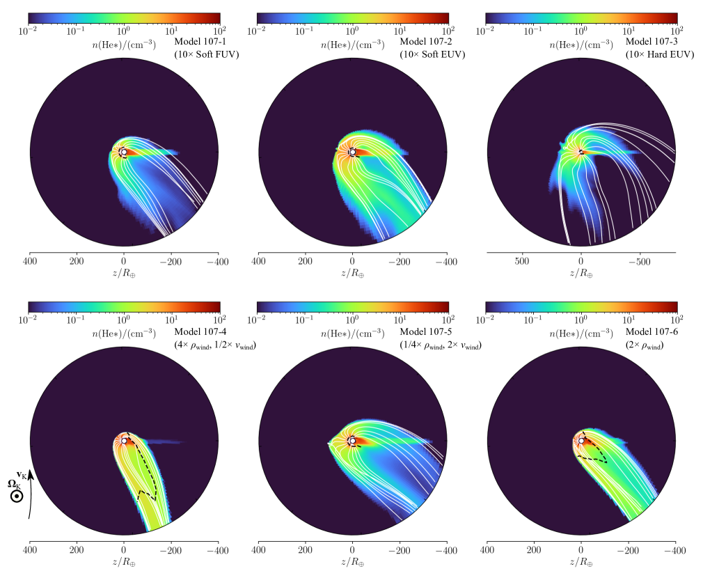
Figure 7: $\mathrm{He}^{*}$ number density profiles in the orbital plane, with streamlines (spaced with the same scheme as Figure 2) and sonic surfaces overlaid. The panel for Model 107-3 has different spatial scales. Some lines appear to overlap with other lines or to terminate before reaching the outer boundary because the streamlines are projected. Note that Models 107-4 and 107-6 comply with the Case C in Figure 1.

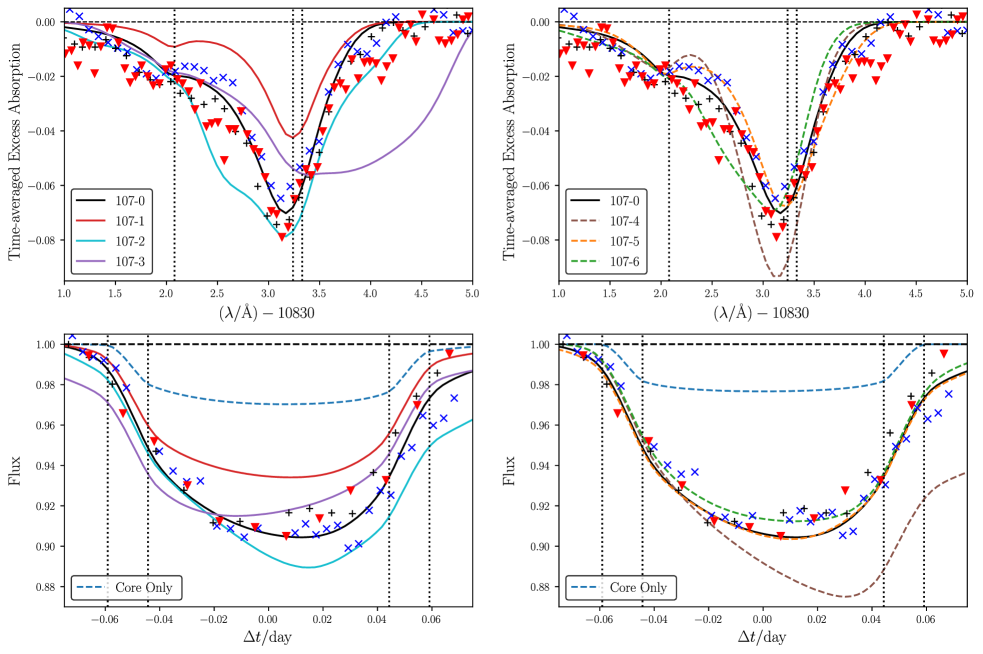
Figure 8: Similar to Figures 4 but for the models in §4.2 and Table 2. Left column compares Models 107-1 through 107-3 to the fiducial 107-0, and the right column does the comparison for Models 107-4 through 107-6 to 107-0. The window function for the light curves are the same as the one used to yield Figure 4.

Table 2: Results of various models, based on the fiducial model for WASP-107b

Model	Description	$\dot{M}$	$\langle W_{\lambda}\rangle$	$\Delta v_{\rm peak}$	FWHM
		($10^{-9}~{}M_{\oplus}~{}\mathrm{yr}^{-1}$)	($10^{-2}~{}\text{\AA}$)	($\mathrm{km}~{}\mathrm{s}^{-1}$)	($\mathrm{km}~{}\mathrm{s}^{-1}$)
107-0	Fiducial	$1.02\pm 0.01$	$7.6\pm 0.2$	$-3.5$	$22.7$
107-1	$10\times$ Flux at $h\nu=7~{}\mathrm{eV}$	$1.09\pm 0.01$	$3.7\pm 0.1$	$-1.7$	$17.2$
107-2	$10\times$ Flux at $h\nu=20~{}\mathrm{eV}$	$1.23\pm 0.01$	$11.3\pm 0.9$	$-3.7$	$34.6$
107-3	$10\times$ Flux at $h\nu=40~{}\mathrm{eV}$	$3.47\pm 0.03$	$12.1\pm 1.1$	$2.4$	$55.1$
107-4	$4\times\rho_{\mathrm{wind}}$, $1/2\times v_{\mathrm{wind}}$	$0.98\pm 0.02$	$8.6\pm 0.1$	$-4.5$	$20.4$
107-5	$1/4\times\rho_{\mathrm{wind}}$, $2\times v_{\mathrm{wind}}$	$1.02\pm 0.01$	$7.4\pm 0.4$	$-2.3$	$22.6$
107-6	$2\times\rho_{\mathrm{wind}}$	$0.99\pm 0.02$	$8.2\pm 0.1$	$-5.6$	$28.2$

Note. — The values and errors are time averages and three times the standard deviations ($3\sigma$), respectively; the time averages are taken over the last $25~{}\tau_{\mathrm{dyn}}$ of the simulations.

4 Parametric Studies

The previous section elaborates the fiducial model for WASP-107b. We found that, by including stellar winds, the simulation quantitatively reproduces various observed features of the $\mathrm{He}^{*}$ transits. This section investigates how the outflow morphology and $\mathrm{He}^{*}$ observables are affected by each model parameter (Figures 7 and 8). We set a series of models, each differs from the fiducial model by one parameter only unless specifically indicated. Table 2 and Figure 8 summarize the models and their corresponding key $\mathrm{He}^{*}$ observables.

4.1 High-Energy Radiation Fluxes

Paper I found that $\mathrm{He}^{*}$ transit observation are primarily determined by soft FUV (which destroys the $\mathrm{He}^{*}$ state) and the EUV bands (which is most important in driving the photoevaporative outflow; interested readers are referred to Paper I for more details); the Lyman-Werner and X-ray bands play secondary roles. We found very similar results for WASP-107b after including stellar winds, by running a separate test simulation excluding X-ray photons (not presented in this paper) that yields almost identical morphology and observables to the fiducial one. In Model 107-1 through 107-3, we raise stellar fluxes in the soft FUV ($h\nu=7~{}\mathrm{eV}$), soft EUV ($20~{}\mathrm{eV}$), and hard EUV ($40~{}\mathrm{eV}$) bands, respectively.

Model 107-1 increases the soft FUV flux by a factor of 10. As we have noted earlier, soft FUV does not inject significant heat into the atmosphere and has minor effects in driving the planetary outflow. Its mass loss rate is very similar to that in the fiducial model [$(\dot{M}/10^{-9}~{}M_{\oplus}~{}\mathrm{yr}^{-1})=1.08$ versus $1.02$]. Soft FUV is nonetheless capable of photoionizing the $\mathrm{He}^{*}$ state efficiently, slicing the equivalent widths by a factor of 2 [$(\langle W_{\lambda}\rangle/10^{-2}~{}\text{\AA}=3.7$ versus 7.6). Models 107-2 and 107-3 raise the soft and hard EUV flux level by a factor of 10, respectively. As expected, intense EUV fluxes boosted the photoevaporation rates, indicated by the stronger mass loss rate and equivalent width. What is curious, however, is that in 107-3, the planetary outflow is so strong that it is push back the bow shock with stellar wind on the day-side to much higher altitudes. In order to fully contain the pushed-back contact surface and the bow shock, we use $r_{\rm out}=800~{}R_{\oplus}$ for the outer radial boundary of 107-3. This effect is so strong that we begin to see the day-side (pre-ingress) material in redshift, and the overall $\mathrm{He}^{*}$ line profile is now biased towards the red wing (Figure 8, upper panel). This strong day-side outflow also manifests as a reversed asymmetry in the $\mathrm{He}^{*}$ light curve, where the ingress is more extended and stronger than the egress (Figure 8, lower panel). This qualitative change in behavior will possibly constrain the balance of high-energy radiation strengths between the stellar wind and the planetary outflow.

4.2 How Stellar Winds Shape Outflows

In hydrodynamic simulations (no magnetic effects included), the interactions between stellar winds and planetary outflows should be determined by the wind ram pressure ($\sim\rho_{\mathrm{wind}}v_{\mathrm{wind}}^{2}$), as a function of the density ($\rho_{\mathrm{wind}}$) and velocity ($\vec{v}_{\mathrm{wind}}$). Fortunately, this degeneracy between wind density and velocity can be potentially broken by orbital motion, i.e. the headwind component of the stellar wind.

On one hand, Model 107-4 quadruples the density $\rho_{\mathrm{wind}}$ and halves the velocity $v_{\mathrm{wind}}$, thus keeping the radial (from host to planet) component of ram pressure roughly the same as in the fiducial model. The headwind component, caused by the Keplerian motion $v_{\mathrm{K}}$ of the planet, is held constant here. Lower velocity shear yields a less turbulent trailing tail with weaker shear instabilities. As a result, the tail lags behind the planet in both velocity and spatial sense, producing a more blueshifted line profile [$(\Delta v_{\rm peak}/\mathrm{km}~{}\mathrm{s}^{-1})=-4.5$, versus $-3.5$ for the fiducial], and a more asymmetric light curve. On the other hand, in Model 107-5 which doubles the velocity but quartered the density, the tail is now influenced by the radial component more heavily. It is primarily directed towards the night-side, and displays considerably more vigorous shear instabilities due to greater velocity shears. The $\mathrm{He}^{*}$ light curve has much weaker post-egress absorption, while the equivalent width sees more variability [$(\langle W_{\lambda}\rangle/10^{-3}\text{\AA})=7.4\pm 0.4$, versus $7.6\pm 0.2$ in the fiducial model]. Finally, Model 107-6, only increases the density $\rho_{\mathrm{wind}}$ by a factor of two. Having the same ratio of $v_{\mathrm{wind}}/v_{\mathrm{K}}$ as in the fiducial model, Model 107-6 produces a tail that has similar direction as the fiducial model. Increased ram pressure still pushes the outflow to greater blueshift velocities [$(\Delta v_{\rm peak}/\mathrm{km}~{}\mathrm{s}^{-1})=-5.6$ versus $-3.5$].

5 Discussions

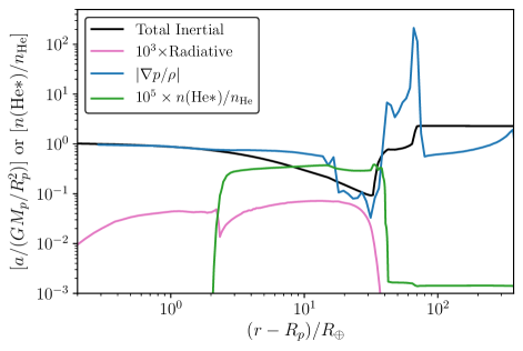
Figure 9: Profiles of acceleration magnitudes (normalized by $GM_{\rm p}/R_{\rm p}^{2}$) that contains extra photon energy bins at Ly$\alpha~{}$and $10833~{}\text{\AA}$ radiated by the host star. Inertial acceleration (including planet and stellar gravity, centrifugal force, and Coriolis force), radiation pressure acceleration (multiplied by $10^{3}$) and pressure gradient acceleration profiles are measured along the $\theta=\pi/4$, $\phi=0$ radial line. The Radiation pressure profile is multiplied by $10^{3}$ for clearer presentation. As a reference, the relative abundance of $\mathrm{He}^{*}$ (multiplied by $10^{5}$) is also shown.

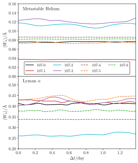
Figure 10: Temporal variation of the equivalent widths of the metastable helium absorption lines (upper panel) and Ly$\alpha~{}$(lower panel), for the models described in Table 2. Such fluctuations are mainly the results of the instabilities emerging in the interactions between stellar wind and planetary outflows. For each simulation, the last $1.4~{}{\rm day}\sim 25~{}\tau_{\mathrm{dyn}}$ of its simulated time duration is shown.

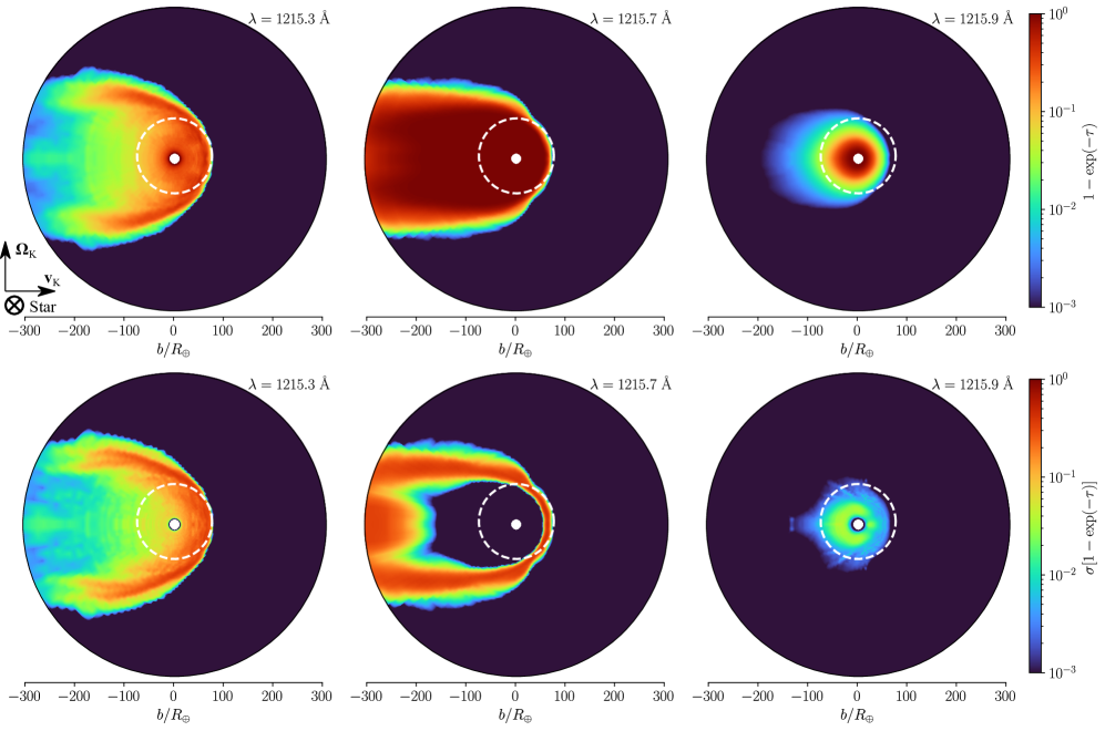
Figure 11: Similar to Figure 6 but for the wavelengths $(\lambda/\text{\AA})\in\{1215.3,1215.7,1215.9\}$ near the Ly$\alpha~{}$line.

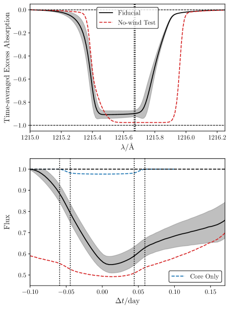
Figure 12: Similar to Figure 4 but for the Ly$\alpha~{}$synthetic spectra based on Model 107-0 and its corresponding test models only. The wavelength window for the light curves is $(\lambda/\text{\AA})\in[1215.0,1216.25]$. Note that the line profiles in the upper panel has a saturated shape but the excess absorption does not reach $\langle\Delta\epsilon\rangle=-1$, because (1) the extinction by planet core is subtracted from the total absorption, and (2) the full ingress of the Ly$\alpha~{}$absorption region is delayed by the stellar wind.

5.1 Tail: Stellar Wind or Radiation Pressure?

As we have shown in the previous sections, the existing $\mathrm{He}^{*}$ observations of WASP-107b are suggestive of a comet-like tails that trail the photoevaporating planet. What is the mechanism that give rise to these tails? Is it stellar wind or radiation pressure or a combination of these two effects? When studying the Ly$\alpha~{}$outflow for exoplanets, previous studies often attributed transit asymmetry to radiation pressure (e.g. Bourrier et al., 2015, 2016). Recent works in $\mathrm{He}^{*}$ followed suit: in an EVE simulation of WASP-107b (a collisionless particle-based simulations; Allart et al. 2018, 2019), the authors found that their prescription of radiation pressure accelerates the outflow way too quickly, producing a tail that is directly pointing away from the night-side of the planet. Their prescribed effect of radiation pressure is so strong that the authors had to artificially decrease the stellar spectrum near the $\mathrm{He}^{*}$ lines by a factor 50 to achieve reasonable agreement with the observations of WASP-107b. We argue, in this work, that their particle-based simulation is not adequate to account for the effect of radiation pressure on $\mathrm{He}^{*}$ transitions.

We must first clearly distinguish the Ly$\alpha~{}$transition and the $\mathrm{He}^{*}$ transitions. The lower state of Ly$\alpha~{}$is the ground state of neutral hydrogen, while $\mathrm{He}^{*}$ (i.e. the $2^{3}$S state of helium) is relatively much more difficult to populate, and has a much lower abundances throughout the domain of interest ($\lesssim 10^{-5}$, Figure 3; see also Paper I; Oklopčić 2019). Meanwhile, the product of Einstein $A$ coefficient and the overall element abundance for helium is also $\sim 10^{2}$ times smaller than Ly$\alpha~{}$. Consequently, the altitude where most $\mathrm{He}^{*}$ absorption occurs is often much lower than Ly$\alpha~{}$absorption region. The gas density in these regions is significantly higher, and the mean free path (MFP) of momentum transfer are much shorter. In our simulations, we typically see $n(\mathrm{H}^{+})\gtrsim 10^{6}~{}\mathrm{cm}^{-3}$, and an MFP of $\lambda=1/[n(\mathrm{H}^{+})\sigma]\lesssim 10^{3}~{}\mathrm{cm}$ (see also Thomas & Humberston, 1972; Draine, 2011). This is $\sim 6$ orders of magnitude smaller than the hydrodynamic length scales. Such a contrast in length scales demands a hydrodynamic treatment, instead of a collisionless particle-based one. What is more, the momenta deposited into $\mathrm{He}^{*}$ by absorption are quickly diluted and thermalized by more collisions. In contrast, the collisionless particle-based treatment such as EVE is more appropriate for simulating the Ly$\alpha~{}$outflow, since the density where most Ly$\alpha~{}$absorption occurs is much lower: in our simulations, we have $n(\mathrm{H}^{+})\lesssim 10^{-1}~{}\mathrm{cm}^{-3}$ and the MFP is $\lambda\sim 10^{10}~{}\mathrm{cm}\sim 10~{}R_{\oplus}$. Neutral hydrogen atom there are essentially decoupled from other components of the gas, and are indeed susceptible to the momentum deposited by the absorption of Ly$\alpha~{}$. Nonetheless, as far as the $\mathrm{He}^{*}$ observations are concerned, the radiation pressure on Ly$\alpha~{}$can be safely ignored.

Figure 9 compares the magnitudes of acceleration (force per unit mass) by radiation pressure (where most $\mathrm{He}^{*}$ absorption occurs), gas pressure gradient, and inertial force (including stellar and planetary gravitation, centrifugal force, and Coriolis force). Radiation pressure in this model is more than three orders of magnitude weaker than the pure hydrodynamic effects. Again, the high density of $\mathrm{He}^{*}$ absorbing region maintains sufficiently strong momentum coupling of different species and guarantees quick dilution of the momenta injected by Ly$\alpha~{}$photons. The photons here heat rather than push the planetary outflow.

In addition, we set up a verification test simulation to numerically examine the effect of radiation pressure. We added two more photon energy bins in our ray-tracing radiative transfer module: one has $h\nu=10.2~{}\mathrm{eV}$ for Ly$\alpha~{}$, and $h\nu=1.15~{}\mathrm{eV}$ for the metastable helium lines whose flux is of a typical K-type stars (Wood et al., 2005). For simplicity, we assume that the cross-sections for photon momentum absorption for these two energy bins are equal to the line-center value, and we ignored the dispersion of photons in the frequency space. We note that these assumptions should only amplify the effects of radiation pressure. This simulation produced almost identical result as a no-radiation-pressure model in terms of hydrodynamic and thermochemical profiles, as well as $\mathrm{He}^{*}$ observables.

In summary, at least for $\mathrm{He}^{*}$ lines, radiation pressure only plays a minor role in shaping the outflow morphology and kinematics. Stellar wind, as we have shown in previous section, is essential in reproducing various observed features $\mathrm{He}^{*}$ transitions. We propose that, should future observation of $\mathrm{He}^{*}$ show strong deviations from a “quiescent” line ratio ($\sim 1:8$) or an asymmetry in line profile or light curve, it may be regarded as an indication of stellar winds, whose properties can be constrained with detailed 3D hydrodynamic simulations.

5.2 Shear Instability

At the contact surface that separates the stellar wind and the photoevaporative outflow, there is region of large shears in velocity. Shear instabilities are generated here, manifesting themselves as billowing outflows. We found that since the sonic surface is located at much lower altitude (Figure 1; see also Figure 3), the outflow mass-loss rate is not affected by these shear instabilities. If the host star high-energy SED is held constant, the mass loss rate stays rather stable ($<1~{}\%$ fluctuation) at about $\dot{M}\simeq 1.02\times 10^{-9}~{}M_{\oplus}~{}\mathrm{yr}^{-1}$ in our fiducial model of WASP-107b. However, the $\mathrm{He}^{*}$ absorption takes place at higher altitudes (Figure 6), and is directly influenced by shear instabilities. Fluctuations of transit depths have relative amplitudes $\sim 5~{}\%$ to $\sim 20~{}\%$ at different wavelength, while the typical timescale is $\sim 0.2~{}{\rm day}$ (Figure 10). In contrast, in our WASP-69b model in Paper I, shear instabilities are not excited since stellar wind was not included. $\mathrm{He}^{*}$ absorption shows a $\lesssim 0.5~{}\%$ temporal variations.

An interesting prediction associated with shear instability is that there should be much stronger fluctuations in the blueshifted wings of $\mathrm{He}^{*}$ line profiles. Moreover, in the $\mathrm{He}^{*}$ light curve, the variability should be much stronger after the mid-transit point. The reason is that shear instability takes time and space to grow: its spatial extent is still small in the redshifted head part of the outflow, but fully developed when it enters the blueshifted tail. In Figure 4, the gray shaded region indicates the amplitudes of variability due to shear billows, and clearly demonstrates this fluctuation-induced asymmetry. Up to the composition of this paper, two $\mathrm{He}^{*}$ transits have been reported; more transits, preferably from the same instruments, are needed to evaluate the fluctuation asymmetries.

5.3 Line Ratio Probes Kinematics Instead of Density

It has been suggested that the line ratios between three transition of the $\mathrm{He}^{*}$ can tell us about the density of the underlying outflow. If all three lines are not saturated, the line ratios between the triplet should be proportional to 1:3:5, or their quantum degeneracies. Considering that the two longer-wavelength transitions are often blended together thermally and kinematically, the line ratio should be 1:8. Now if the density of the outflow is high enough that the transitions start to saturate, the line ratio may begin to deviate from 1:8 and hint us about the number density of $\mathrm{He}^{*}$ in the outflow. However, as we have seen in Paper I for WASP-69b, most of the $\mathrm{He}^{*}$ extinction happens at high-altitude, low-density regions of $10^{1-2}~{}R_{\oplus}$ (see Figure 6, showing the mid-transit extinction at three characteristic wavelengths near the $\mathrm{He}^{*}$ transitions). The lines are far from saturation in these regions. In other words, the line ratios can not directly probe the density distribution at least for WASP-107b.

We do observe a line ratio of about 1:4 in our fiducial model of WASP-107b, which is significantly different from the 1:8 expected by quantum degeneracies. It is noted that this deviation is primarily caused by the kinematics of the outflow: the peak due to two longer-wavelength transitions are blueshifted by the wind by up to $\sim 20-30~{}\mathrm{km}~{}\mathrm{s}^{-1}$, that its blueshifted wing start to invade the shorter-wavelength transition. We will see in the next subsection that the line ratio and the exact shape of the $\mathrm{He}^{*}$ will serve as a probe of the outflow kinematics and in turn the properties of stellar wind.

Here we present an example that one can semi-quantitatively constrain the stellar wind density and velocity using the $\mathrm{He}^{*}$ observation. We shall focus on the contact discontinuity, i.e. the boundary separating the stellar wind and the planetary outflow (Figures 1, 2). The distance of contact discontinuity from the planet can be estimated by equating the total pressure of a photoevaporative outflow to the ram pressure of the stellar wind $\rho_{\mathrm{wind}}v_{\mathrm{wind}}^{2}$:

$$\begin{split}r_{\rm cd}\sim&\left[\dfrac{\dot{M}c_{s}}{\pi\rho_{\mathrm{wind}}v_{\mathrm{wind}}^{2}}\right]^{1/2}\\ \sim&~{}500~{}R_{\oplus}\times\left(\dfrac{\dot{M}}{10^{-9}~{}M_{\oplus}~{}\mathrm{yr}^{-1}}\right)^{1/2}\left(\dfrac{T}{10^{4}~{}\mathrm{K}}\right)^{1/4}\\ &\times\left(\dfrac{\rho_{\mathrm{wind}}}{10^{-20}~{}\mathrm{g}~{}\mathrm{cm}^{-3}}\right)^{-1/2}\left(\dfrac{v_{\mathrm{wind}}}{100~{}\mathrm{km}~{}\mathrm{s}^{-1}}\right)^{-1}\ ,\end{split}$$ (2)

where the subscript “cd” stands for the contact discontinuity. In our fiducial model, this estimation yields $r_{\rm cd}\sim 45~{}R_{\oplus}$ with the parameters in Table 1. This is reasonably accurate with visual inspection of Figure 2. We note that if the stellar wind intensity is similar to the Sun at an $a=0.055~{}\mathrm{AU}$ orbit, which roughly has $\rho_{\mathrm{wind}}\sim 3\times 10^{3}~{}m_{p}~{}\mathrm{cm}^{-3}$ and $v_{\mathrm{wind}}\sim 300~{}\mathrm{km\ s^{-1}}$ at $\sim 0.05~{}\mathrm{AU}$ (see Venzmer & Bothmer 2018 and references therein), $r_{\rm cd}\sim 240~{}R_{\oplus}$ would be inconsistent with the observations on WASP-107b. Such stronger stellar wind experienced by WASP-107b is perhaps not surprising, given its closer-in orbit, and the relative youth and higher activity of the host star.

5.4 Synergy between Ly$\alpha~{}$and $\mathrm{He}^{*}$ Observations

This section briefly discusses how observing transits of an exoplanets in both Ly$\alpha~{}$and $\mathrm{He}^{*}$ can be synergistic in helping us understand its atmospheric outflow. First of all, we reiterate the point made in §5.1 that most Ly$\alpha~{}$absorption happens at much higher altitudes than $\mathrm{He}^{*}$ absorption. The low density at higher altitude means that Ly$\alpha~{}$radiation pressure may start to reshape the morphology of neutral hydrogen; while the at lower altitude of $\mathrm{He}^{*}$ absorption, radiation pressure heats rather than pushes the planetary outflow. This potentially allows us to disentangle the influence of radiation pressure and stellar wind, and disentangle the inner and outer parts of the planet outflow.

We produced synthetic line profiles and light curves in the Ly$\alpha~{}$band for WASP-107b in Figure 12 and Figure 11. Note that we did not account for the extinction due to the interstellar medium. We also note that Ly$\alpha~{}$observations are currently unavailable for WASP-107b and will probably remain the case given the distant host and the expected strong UV extinction. However, we still notice that the line profile is blueshifted significantly while Ly$\alpha~{}$light curve shows much more pronounced asymmetry with elongated egress. Both of these observations are qualitatively similar to other exoplanets observed in Ly$\alpha~{}$(e.g., GJ 436b; see also Ehrenreich et al. 2015; Bourrier et al. 2015, 2016). It is also curious that radiation pressure alone could not produce as strong as an asymmetry produced by stellar wind. The no-wind model produces deep Ly$\alpha~{}$transit light curve that ingress and egress elongated to similar extent. Another prediction we can predict from joint Ly$\alpha~{}$and $\mathrm{He}^{*}$ is that the absorption fluctuation due to shear instabilities should be stronger in Ly$\alpha~{}$than in $\mathrm{He}^{*}$; and Ly$\alpha~{}$fluctuations should lag behind $\mathrm{He}^{*}$ fluctuations. The reason is, again, most Ly$\alpha~{}$absorption happen at higher altitude than $\mathrm{He}^{*}$ absorption. Instabilities grows as it propagates from lower altitude region to higher altitudes. The shaded bands in Figure 12 illustrate the simulated variations in Ly$\alpha~{}$absorption.

Some of the points raised here were also suggested by McCann et al. (2019) who focused hot Jupiters. After all, transit observations in $\mathrm{He}^{*}$ and Ly$\alpha~{}$, particularly multiple simultaneous transit observations, will be instrumental in helping us understand the morphology and kinematics of atmospheric loss on different spatial scales. With such observations, we may also acquire more knowledge about the characteristics and variabilities of stellar wind from the host star. Hybrid models combining hydrodynamics with particles-based simulations are perhaps mandatory to fully characterize the various species of the outflow at highest altitude especially neutral hydrogen.

6 Summary

This paper presents simulations of the metastable helium absorption lines in the transmission of WASP-107b. We employ full 3D hydrodynamic simulations to model the dynamics of evaporating planetary atmospheres, in which non-equilibrium thermochemistry and ray-tracing radiative transfer are co-evolved. The processes that populate and de-populate the metastable state of neutral helium are included in the thermochemical network and solved consistently. These allow us to predict the mass loss rate, the temperature profile, and synthetic observation in both Ly$\alpha~{}$and $\mathrm{He}^{*}$; we note that previous works often have to assume or prescribe the first two.

By exploring the parameter space, we find a plausible model for WASP-107b that also involves a stellar wind stronger than the solar wind. This model launches a photoevaporative outflow with a mass-loss rate of $\dot{M}\simeq 1.0\times 10^{-9}~{}M_{\oplus}~{}\mathrm{yr}^{-1}$. The predicted $\mathrm{He}^{*}$ line profiles and light curves exhibit reasonable agreement with existing observations. Time-averaged transmission spectrum has a $\sim 1:4>1:8$ line ratio, while the light curve holds a considerable asymmetry about the transit median. A comet-like tail trailing the planet is a natural explanation of these observations. We argue that such a tail is the result of a relatively strong stellar wind rather than radiation pressure, because (1) the low overall abundance of$\mathrm{He}^{*}$, and (2) the photon momenta deposited by absorption and scattering are quickly thermalized by collisional momentum relaxation. The incoming stellar wind triggers shear instabilities, and the $\mathrm{He}^{*}$ transit depth fluctuates by $5-20~{}\%$ at a roughly $\sim 0.2~{}{\rm day}$ timescale consequently. Tuning the characteristics of stellar wind in a plausible range does affect the spectral line shapes through alternating the direction and configuration of the tail, yet the equivalent width is largely invariant. The Ly$\alpha~{}$transmission spectra and light curve synthesized using the fiducial Model 107-0 suggest stronger light curve asymmetry and variabilities due to shear instabilities. We propose that surveys of exoplanets in Ly$\alpha~{}$and $\mathrm{He}^{*}$ simultaneously are crucial for understanding planetary outflow and stellar wind.

Looking ahead, planetary outflow modulated by stellar winds may extract positive or negative orbital angular momentum from the planet via dynamical (anti-)friction (Li et al., 2020), and may then lead to migrations of planetary orbits. Planetary magnetic fields and the fields carried by stellar winds or coronal ejecta may also play essential roles in shaping the dynamics of an evaporating close-in planet. Future simulations should have magnetohydrodynamics involved in these processes with improved consistency, and potentially shed light on the evolution of magnetic fields when compared to observations.

This work is supported by the Center for Computational Astrophysics of the Flatiron Institute, and the Division of Geological and Planetary Sciences of the California Institute of Technology. L. Wang acknowledges the computing resources provided by the Simons Foundation and the San Diego Supercomputer Center. We thank our colleagues (alphabetical order): Philip Armitage, Zhuo Chen, Jeremy Goodman, Xinyu Li, Mordecai Mac-Low, Songhu Wang, and Andrew Youdin, for helpful discussions and comments.

References

- Allart et al. (2018) Allart, R., Bourrier, V., Lovis, C., et al. 2018, Science, 362, 1384, doi: 10.1126/science.aat5879
- Allart et al. (2019) —. 2019, A&A, 623, A58, doi: 10.1051/0004-6361/201834917
- Anderson et al. (2017) Anderson, D. R., Collier Cameron, A., Delrez, L., et al. 2017, A&A, 604, A110, doi: 10.1051/0004-6361/201730439
- Bourrier et al. (2015) Bourrier, V., Ehrenreich, D., & Lecavelier des Etangs, A. 2015, A&A, 582, A65, doi: 10.1051/0004-6361/201526894
- Bourrier et al. (2016) Bourrier, V., Lecavelier des Etangs, A., Ehrenreich, D., Tanaka, Y. A., & Vidotto, A. A. 2016, A&A, 591, A121, doi: 10.1051/0004-6361/201628362
- Chachan et al. (2020) Chachan, Y., Jontof-Hutter, D., Knutson, H. A., et al. 2020, AJ, 160, 201, doi: 10.3847/1538-3881/abb23a
- Dai & Winn (2017) Dai, F., & Winn, J. N. 2017, AJ, 153, 205, doi: 10.3847/1538-3881/aa65d1
- Draine (2011) Draine, B. T. 2011, Physics of the Interstellar and Intergalactic Medium (Princeton University Press)
- Drake (1971) Drake, G. W. 1971, Phys. Rev. A, 3, 908, doi: 10.1103/PhysRevA.3.908
- Ehrenreich et al. (2015) Ehrenreich, D., Bourrier, V., Wheatley, P. J., et al. 2015, Nature, 522, 459, doi: 10.1038/nature14501
- France et al. (2016) France, K., Loyd, R. O. P., Youngblood, A., et al. 2016, ApJ, 820, 89, doi: 10.3847/0004-637X/820/2/89
- Gao & Zhang (2020) Gao, P., & Zhang, X. 2020, ApJ, 890, 93, doi: 10.3847/1538-4357/ab6a9b
- Gudel (1992) Gudel, M. 1992, A&A, 264, L31
- Kirk et al. (2020) Kirk, J., Alam, M. K., López-Morales, M., & Zeng, L. 2020, AJ, 159, 115, doi: 10.3847/1538-3881/ab6e66
- Kreidberg et al. (2018) Kreidberg, L., Line, M. R., Thorngren, D., Morley, C. V., & Stevenson, K. B. 2018, ApJ, 858, L6, doi: 10.3847/2041-8213/aabfce
- Li et al. (2020) Li, X., Chang, P., Levin, Y., Matzner, C. D., & Armitage, P. J. 2020, MNRAS, 494, 2327, doi: 10.1093/mnras/staa900
- Libby-Roberts et al. (2020) Libby-Roberts, J. E., Berta-Thompson, Z. K., Désert, J.-M., et al. 2020, AJ, 159, 57, doi: 10.3847/1538-3881/ab5d36
- Loyd et al. (2016) Loyd, R. O. P., France, K., Youngblood, A., et al. 2016, ApJ, 824, 102, doi: 10.3847/0004-637X/824/2/102
- McCann et al. (2019) McCann, J., Murray-Clay, R. A., Kratter, K., & Krumholz, M. R. 2019, ApJ, 873, 89, doi: 10.3847/1538-4357/ab05b8
- Ninan et al. (2020) Ninan, J. P., Stefansson, G., Mahadevan, S., et al. 2020, ApJ, 894, 97, doi: 10.3847/1538-4357/ab8559
- Nortmann et al. (2018) Nortmann, L., Pallé, E., Salz, M., et al. 2018, Science, 362, 1388, doi: 10.1126/science.aat5348
- Oklopčić (2019) Oklopčić, A. 2019, ApJ, 881, 133, doi: 10.3847/1538-4357/ab2f7f
- Oklopčić & Hirata (2018) Oklopčić, A., & Hirata, C. M. 2018, ApJ, 855, L11, doi: 10.3847/2041-8213/aaada9
- Parker (1958) Parker, E. N. 1958, ApJ, 128, 664, doi: 10.1086/146579
- Salz et al. (2018) Salz, M., Czesla, S., Schneider, P. C., et al. 2018, A&A, 620, A97, doi: 10.1051/0004-6361/201833694
- Seager & Sasselov (2000) Seager, S., & Sasselov, D. D. 2000, ApJ, 537, 916, doi: 10.1086/309088
- Spake et al. (2018) Spake, J. J., Sing, D. K., Evans, T. M., et al. 2018, Nature, 557, 68, doi: 10.1038/s41586-018-0067-5
- Thomas & Humberston (1972) Thomas, M. A., & Humberston, J. W. 1972, Journal of Physics B: Atomic and Molecular Physics, 5, L229, doi: 10.1088/0022-3700/5/11/002
- Turner et al. (2016) Turner, J. D., Christie, D., Arras, P., Johnson, R. E., & Schmidt, C. 2016, MNRAS, 458, 3880, doi: 10.1093/mnras/stw556
- Venzmer & Bothmer (2018) Venzmer, M. S., & Bothmer, V. 2018, A&A, 611, A36, doi: 10.1051/0004-6361/201731831
- Wang & Dai (2019) Wang, L., & Dai, F. 2019, ApJ, 873, L1, doi: 10.3847/2041-8213/ab0653
- Wood et al. (2005) Wood, B. E., Redfield, S., Linsky, J. L., Müller, H.-R., & Zank, G. P. 2005, ApJS, 159, 118, doi: 10.1086/430523
- Youngblood et al. (2016) Youngblood, A., France, K., Loyd, R. O. P., et al. 2016, ApJ, 824, 101, doi: 10.3847/0004-637X/824/2/101
- Youngblood et al. (2017) —. 2017, ApJ, 843, 31, doi: 10.3847/1538-4357/aa76dd