TTP19-025

P3H-20-085

RGE++
A C++ library to solve renormalisation group equations in quantum field theory

Thomas Deppisch${}^{\,a}$ , Florian Herren${}^{\,b}$

^a German Weather Service (DWD)

Research and Development — Data Assimilation

Frankfurter Straße 135, D-73067 Offenbach am Main, Germany

^b Institut für Theoretische Teilchenphysik

Karlsruhe Institute of Technology (KIT)

Wolfgang-Gaede-Straße 1, D-76128 Karlsruhe, Germany

In recent years three-, four- and five-loop beta functions have been computed for various phenomenologically interesting models. However, most of these results have not been implemented in easy to use software packages. RGE++ bridges this gap by providing a flexible, template-based, C++ library to solve renormalisation group equations. Furthermore, we implement the available beta functions for the Standard Model, the minimal supersymmetric extension of the Standard Model and two-Higgs-doublet models, as well as right-handed neutrino extensions of the former two.

1 Introduction

When renormalised in the modified minimal subtraction ($\overline{\mathrm{MS}}$) or modified dimensional reduction ($\overline{\mathrm{DR}}$) schemes, parameters and fields in quantum field theories depend on the renormalisation scale $\mu$. The change of a parameter with respect to a change of $\mu$ is encoded in anomalous dimensions, or, in the case of coupling constants, the beta functions

$$\frac{\mathrm{d}}{\mathrm{d}\ln\mu}g_{i}=\beta_{g}\left(\left\{g_{j}\right\}\right)~{},$$ (1)

where the $g_{i}$ denote any dimensionless coupling of the theory under consideration and $\left\{g_{j}\right\}$ denotes the set of all couplings of the theory. Beta functions play a crucial role in connecting parameters at different scales, for example when comparing measurements of the strong coupling constant at different energy scales at the Z-Boson mass $\mu=M_{Z}$. Other applications include the study of Grand Unified Theories (GUTs) by extrapolating the measured couplings at low scales to the unification scale or the generation of supersymmetric (SUSY) spectra from high-scale input.

Usually, Eq. (1) is solved numerically and over the years many public programs appeared which implement anomalous dimensions and beta functions of various models. Most of them implement more features than the scope of RGE++, but are rather specific to a certain model. Here we provide a short overview of programs or libraries which are relevant in the context of renormalisation group equations (RGEs): For pure QCD at the highest perturbative orders available there is (C)RunDec [1, 2, 3]. SMDR [4] and mr [5] implement running and matching relations in the full Standard Model, while REAP [6] implements beta functions in the SM, MSSM and 2HDMs including right-handed neutrinos. For supersymmetric theories there is a plethora of spectrum generators, which all implement various models, such as SOFTSUSY [7], SuSpect [8], SPheno [9, 10], Flexible SUSY [11, 12]. Furthermore, there are programs implementing the general two-loop beta functions [13, 14, 15, 16, 17, 18] and anomalous dimensions of the dimensionful couplings [19, 20], such as SARAH [21], PyR@TE [22, 23] and ARGES [24].

The goal of RGE++ is much simpler: to provide an easy to use, template-based C++ class library, capable of numerically solving rather generic RGEs, which can be used from within other programs. Furthermore, we want to provide various higher-order results, since many of the aforementioned programs only implement the relevant beta functions and anomalous dimensions up to two loops.

Given recent developments such as the extraction of the gauge coupling beta function in a general quantum field theory at three loops [26, 25], the computation of the gauge coupling beta functions in the SM at four loops [27], as well as the identification of all colour structures appearing in the four-loop gauge and three-loop Yukawa coupling beta functions, we can expect a plethora of new results for various models. A flexible code such as RGE++ will be able to incorporate such new results quickly.

The remainder of this paper is structured as follows: In Section 2 we present the base classes and discuss the models implemented. Section 3 showcases the usage of RGE++ with four examples. A brief summary, as well as an outlook on further developments can be found in 4.

2 The RGE++ classes and functions

In this section we discuss the functionality of RGE++ and its implementation. Readers who are more interested in actual examples are encouraged to skip ahead to Section 3 and come back to this section afterwards.

First, in Sec. 2.1, we describe the installation and the dependencies of RGE++, followed by a brief overview about the implemented models in Sec. 2.3. The description of the base classes all models are derived from can be found in Sec. 2.4. In Sec. 2.5 we discuss the implementation of the various models and fix the conventions. We conclude with documenting auxiliary functions in Sec. 2.6.

2.1 Installation and usage

The code can be obtained from https://github.com/Herren/RGEpp and is structured as follows: the folders include and src contain the header and source files of the basic classes, respectively. models contains the code for all implemented models, while examples contains the code for various examples, including those documented in the following.

To use RGE++ an installation of the libraries Eigen3 [28] and odeint [29] is necessary. Eigen3 provides template-based implementations of vector and matrix classes. odeint implements standard algorithms for numerically solving differential equations and can operate on the matrix classes provided by Eigen3. They can be obtained by following the instructions in the README file. For building the examples, the variables EIGENPATH and ODEINTPATH in the Makefile might need to be changed accordingly.

2.2 General structure

The source code of RGE++ is distributed over four folders:

• include: contains header files of template and auxiliary classes

• src: contains source files of auxiliary classes

• models: contains model implementations

• examples: contains examples showcasing the use of RGE++

All models are derived from two template classes with a flexible number of gauge and quartic couplings: base and nubase. The latter extends the former by additional matrices to account for neutrino Yukawa couplings and Majorana masses. Both template classes provide all routines and operators for solving the RGEs numerically using odeint.

Specific models are derived from either of the two base classes and implement the operator

⬇

void operator()(const class & X, class & dX, const double)

This operator is called by odeint at each step of the numerical integration, writing the derivative of X into dX. Thus for each model, this operator needs to implement the beta functions of the model. A more detailed discussion is given in Sec. 3.

2.3 Overview of implemented models

RGE++ implements the SM beta functions for gauge couplings, Yukawa matrices and the scalar quartic coupling up to three loops [13, 14, 15, 30, 31, 32, 33, 34, 35, 36, 37, 38, 39]. Furthermore, the four-loop corrections to the gauge coupling beta functions [27] are available. The non-supersymmetric extensions implemented are the SM including right-handed neutrinos at two-loop order [13, 14, 15, 6, 40], as well as the $\mathbb{Z}_{2}$-symmetric two-Higgs-doublet models at three-loop order for gauge coupling and Yukawa matrices and two-loop order for the quartic couplings [13, 14, 15, 36, 41]. The beta functions for the minimal supersymmetric extension of the SM are implemented up to three-loop order [42, 43] and its extension with right-handed (s)neutrinos at two-loop order [42, 6, 44]. All implemented models employ $\mathrm{SU}(5)$ normalization for the $\mathrm{U}(1)_{\mathrm{Y}}$ gauge coupling $g_{1}$.

A full list, including all references, can be found in Table 1.

file name	loop order	publications
sm.h	2	[29, 28, 13, 14, 15]
sm.h	3	[29, 28, 13, 14, 15, 30, 31, 32, 33, 34, 35, 36, 37, 38, 39]
sm.h	4	[29, 28, 13, 14, 15, 30, 31, 32, 33, 34, 35, 36, 37, 38, 39, 27]
mssm.h	2	[29, 28, 42]
mssm.h	3	[29, 28, 42, 43, 45]
nusm.h	2	[29, 28, 13, 14, 15, 6, 40]
numssm.h	2	[29, 28, 42, 6, 44]
thdmi.h	3	[29, 28, 13, 14, 15, 36, 41]
thdmii.h	3	[29, 28, 13, 14, 15, 36, 41]
thdmx.h	3	[29, 28, 13, 14, 15, 36, 41]
thdmy.h	3	[29, 28, 13, 14, 15, 36, 41]
ckm.h	any	[29, 28, 6]
pmns.h	any	[29, 28, 6]
sm_example.cpp	2	[29, 28, 46, 6, 13, 14, 15]

Table 1: Relevant literature for each implemented model that should be cited together with this work when using RGE++ in scientific publications.

2.4 Base classes

eigentypes.h

sets the type definitions

⬇

template<int n>

using gauge = Eigen::Matrix<double, n,1>;

using yukawa = Eigen::Matrix<std::complex<double>, 3,3>;

template<int n>

using self = Eigen::Matrix<std::complex<double>, n,1>;

where gauge and self represent $n$-dimensional vectors of gauge and quartic couplings, while yukawa represents fixed-size quadratic Yukawa matrices. Furthermore, for each of the aforementioned types, the functions

⬇

typename abs(typename); // returns the coefficient-wise absolute values

bool isnotnan(typename); // checks whether a coupling is ’NaN’

are defined, which are used internally in the routines solving the RGE numerically. The types defined in this header file constitute the basic data types on which the various classes are built.

base.h

defines the class base, which serves as a base class from which all model classes with three Yukawa matrices are derived. The following model parameters are defined as public members:

⬇

gauge<n> g; // vector of gauge couplings

self<m> La; // Higgs self-coupling(s)

yukawa Yu,Yd,Ye; // Yukawa matrices

Here n and m are the template parameters of base, specifying the number of gauge and quartic couplings of the model, respectively. The loop order for the beta functions is via the protected member

⬇

unsigned int nloops; // loop order of the beta functions

In all models derived from base nloops defaults to 2.

base.h defines the following member functions of base as public:

⬇

void setZero() // sets g, La, Yu, Yd, Ye to zero

bool check() // ’true’ if no Landau poles appear and no member is ’NaN’

void setNloops(const unsigned int) // sets the value of nloops

unsigned int getNloops() // returns the current value nloops

Besides, base provides all vector space operations needed for the numerical integration with odeint. The classes sm, thdmi/ii/x/y, mssm are derived from base.

nubase.h

defines the class nubase from which all model classes with four Yukawa matrices, the Wilson coefficient of the Weinberg operator, as well as a Majorana mass for right-handed neutrinos are derived. In analogy to base, it has the following model parameters as public members:

⬇

gauge<n> g; // vector of gauge couplings

self<m> La; // Higgs self-coupling(s)

yukawa Yu,Yd,Ye,Yn; // Yukawa matrices

yukawa Ka,Mn; // Wilson coefficient of the Weinberg operator,

// neutrino mass matrix

The loop order for the beta functions is set via the protected member

⬇

unsigned int nloops; // loop order of the beta functions

In all models derived from nubase nloops defaults to 2. In analogy to base.h, nubase.h defines the following public member functions of nubase

⬇

void setZero(); // sets g, La, Yu, Yd, Ye, Yn, Ka, Mn to zero

bool check(); // ’true’ if no Landau poles appear and no member is ’NaN’

void setNloops(const unsigned int); // sets the value of nloops

unsigned int getNloops(); // returns the current value nloops

and provides all vector space operations needed for the numerical integration with odeint.

Furthermore, the class nubase supports the decoupling of heavy right-handed neutrino. The tree-level matching is performed as described in [6] according to

$$\kappa_{ij}^{\rm low}=\kappa_{ij}^{\rm high}+2\,\bigl{(}Y_{\nu}^{T}\bigr{)}_{in}M_{n}^{-1}\bigl{(}Y_{\nu}\bigr{)}_{nj}\;,$$ (2)

in the basis where Mn is diagonal. Here, $\kappa$ corresponds to Ka, the Wilson coefficient of the Weinberg operator. To this end, the class nubase implements the function

⬇

void integrate_out(int n);

which integrates out the $n^{\mathrm{th}}$ generation (counting from zero) of right-handed neutrinos. Afterwards, the $n^{\mathrm{th}}$ row of $Y_{\nu}$ (counting from zero) is set to zero. In addition,

⬇

Eigen::Vector3d logthresholds();

returns the logarithm of the eigenvalues of the right-handed neutrino mass matrix, while

⬇

yukawa getML(double vev);

yukawa getML(double vev, double tanb);

computes the masses of the light neutrinos. The classes nusm and numssm are derived from nubase.

2.5 Implemented models

sm.h

implements the class sm, which is derived as public from base and therefore has all members and member functions of base. A sm object can be constructed by

⬇

sm() : base<3,1>() {};

sm(const gauge<3> g_in, const std::complex<double> La_in,

const yukawa Yu_in, const yukawa Yd_in, const yukawa Ye_in,

const int nloops_in)

: base<3,1>(g_in, Yu_in, Yd_in, Ye_in, nloops_in) { La[0] = La_in; };

sm(const gauge<3> g_in, const std::complex<double> La_in,

const yukawa Yu_in, const yukawa Yd_in, const yukawa Ye_in)

: base<3,1>(g_in, Yu_in, Yd_in, Ye_in) { La[0] = La_in; };

sm(const base<3,1> &X) : base<3,1>(X) {};

The first constructor initializes the values of all couplings to $0$, whereas in the second and third version the couplings are passed as arguments. The third version sets the number of loops to $2$. Finally, the fourth version serves as copy-constructor. Furthermore, sm provides the operator

⬇

void operator()(const sm &X, sm &dX, const double);

which is implemented in sm.cpp. This operator contains the actual implementation of the beta functions and is called by the odeint routines when running from one scale to another.

In the implementation of the beta functions, the ‘right-left-convention’ for the Yukawa interactions is used

$$\mathcal{L}_{\mathrm{Yukawa}}^{\mathrm{SM}}=-Y_{e}^{ij}\;\overline{e_{R}}_{i}\,\phi^{\dagger}\cdot L_{j}-Y_{d}^{ij}\;\overline{d_{R}}_{i}\,\phi^{\dagger}\cdot Q_{j}-Y_{u}^{ij}\;\overline{u_{R}}_{i}\,Q_{j}^{T}\cdot\varepsilon\cdot\phi+\mathrm{H.c.}~{},$$ (3)

where $\varepsilon=\left(\begin{smallmatrix}0&1\\ -1&0\end{smallmatrix}\right)$, $\cdot$ denotes matrix multiplication and the charge conjugated Dirac spinor is $\psi^{C}=-\mathrm{i}\gamma^{2}\gamma^{0}\psi^{T}$. For the Higgs self-coupling $\lambda$ we have

$$\mathcal{L}_{\mathrm{self}}=-\frac{\lambda}{4}(\phi^{\dagger}\phi)^{2}$$ (4)

La is implemented in base as a vector of std::complex<double>. In sm, therefore, all entries but La[0] are set to zero at construction.

thdm.h

implements the classes thdmi, thdmii, thdmx and thdmy, which denote the four $\mathbb{Z}_{2}$-symmetric 2HDMs. They are derived as public from base and therefore have all members and member functions of base. A Type-I 2HDM, for example, can be initialized by

⬇

thdmi() : base() {};

thdmi(const gauge g_in, const self La_in, const yukawa Yu_in,

const yukawa Yd_in, const yukawa Ye_in, const int nloops_in)

: base(g_in, La_in, Yu_in, Yd_in, Ye_in, nloops_in) {};

thdmi(const gauge g_in, const self La_in, const yukawa Yu_in,

const yukawa Yd_in, const yukawa Ye_in)

: base(g_in, La_in, Yu_in, Yd_in, Ye_in) {};

thdmi(const base &X) : base(X) {};

The only difference w.r.t. the SM case is that the self-couplings now form a vector.

Like in the SM case, we use the ‘right-left-convention’ and take $\phi_{2}$ to be the SM-like doublet. So in the Type-I 2HDM

$$\mathcal{L}_{\mathrm{Yukawa}}^{\mathrm{2HDM,I}}=-Y_{e}^{ij}\;\overline{e_{R}}_{i}\,\phi_{2}^{\dagger}\cdot L_{j}-Y_{d}^{ij}\;\overline{d_{R}}_{i}\,\phi_{2}^{\dagger}\cdot Q_{j}-Y_{u}^{ij}\;\overline{u_{R}}_{i}\,Q_{j}^{T}\cdot\varepsilon\cdot\phi_{2}+\mathrm{H.c.}~{}.$$ (5)

To obtain the other three types, one or two of the occurences of $\phi_{2}$ in the above Lagrangian have to be exchanged for $\phi_{1}$, according to Table 2.

Type	$u_{R}$	$d_{R}$	$e_{R}$
I	$\phi_{2}$	$\phi_{2}$	$\phi_{2}$
II	$\phi_{2}$	$\phi_{1}$	$\phi_{1}$
X	$\phi_{2}$	$\phi_{2}$	$\phi_{1}$
Y	$\phi_{2}$	$\phi_{1}$	$\phi_{2}$

Table 2: Couplings of the scalar doublets to right-handed fermions in the four $\mathbb{Z}_{2}$-symmetric 2HDMs.

For the quartic scalar couplings $\lambda_{i}$ we have

$$\mathcal{L}_{\mathrm{self}}=-\frac{\lambda_{1}}{2}(\phi_{1}^{\dagger}\phi_{1})^{2}-\frac{\lambda_{2}}{2}(\phi_{2}^{\dagger}\phi_{2})^{2}-\lambda_{3}(\phi_{1}^{\dagger}\phi_{1})(\phi_{2}^{\dagger}\phi_{2})-\lambda_{4}(\phi_{1}^{\dagger}\phi_{2})(\phi_{2}^{\dagger}\phi_{1})-\left[\frac{\lambda_{5}}{2}(\phi_{1}^{\dagger}\phi_{2})^{2}+\mathrm{h.c.}\right]~{}.$$ (6)

La is implemented in base as a vector of std::complex<double> with 5 entries.

mssm.h

implements the class mssm, which is derived as public from base. A mssm object can be constructed by

⬇

mssm() : base<3,0>() {};

mssm(const gauge<3> g_in, const yukawa Yu_in, const yukawa Yd_in,

const yukawa Ye_in) : base<3,0>(g_in, Yu_in, Yd_in, Ye_in) {};

mssm(const base<3,0> &X) : base<3,0>(X) {};

Note, that in the case of the MSSM, all quartic self-couplings of the scalars are determined by other couplings, namely gauge and Yukawa couplings. Thus all entries of La are set to zero at construction.

The Yukawa couplings are fixed by the superpotential

$$\mathcal{W_{\mathrm{Yukawa}}}^{\mathrm{MSSM}}=Y_{e}^{ij}\;{e_{R}}_{i}\,H_{1}\cdot\varepsilon\cdot L_{j}\quad+Y_{d}^{ij}\;{d_{R}}_{i}\,H_{1}\cdot\varepsilon\cdot Q_{j}+Y_{u}^{ij}\;{u_{R}}_{i}\,\cdot Q_{j}\cdot\varepsilon\cdot H_{2}\;.$$ (7)

nusm.h

implements the class nusm which corresponds to the SM extended by three generations of right-handed neutrinos. nusm is derived as public from nubase and therefore has all members and member functions of nubase. A nusm object can be constructed by

⬇

nusm() : nubase<3,1>() {};

nusm(const gauge<3> g_in, const std::complex<double> La_in,

const yukawa Yu_in, const yukawa Yd_in, const yukawa Ye_in,

const yukawa Yn_in, const yukawa Ka_in, const yukawa Mn_in)

: nubase<3,1>(g_in, Yu_in, Yd_in, Ye_in, Yn_in, Ka_in, Mn_in)

{La[0] = La_in;};

nusm(const nubase<3,1> &X) : nubase<3,1>(X) {};

The conventions for the Yukawa couplings and self-couplings are those of eqs. (3) and (4).

The conventions for Yn, Ka, Mn are defined through

$$\mathcal{L}_{\kappa}^{SM}=-Y_{\nu}^{ij}\;\overline{N}_{i}\,L_{j}^{T}\cdot\varepsilon\cdot\phi-\frac{1}{2}\,M^{ij}\;\overline{N}_{i}N^{c}_{j}+\frac{\kappa^{ij}}{4}\bigl{(}\overline{L^{c}}_{i}\cdot\varepsilon\cdot\phi\bigr{)}\bigl{(}L_{j}^{T}\cdot\varepsilon\cdot\phi\bigr{)}+\mathrm{H.c.}\;.$$ (8)

numssm.h

implements the class numssm which is derived as public from nubase and therefore has all members and member functions of nubase. A numssm object can be constructed by

⬇

numssm() : nubase<3,0>() {};

numssm(const gauge<3> g_in, const yukawa Yu_in, const yukawa Yd_in,

const yukawa Ye_in, const yukawa Yn_in, const yukawa Ka_in,

const yukawa Mn_in)

: nubase<3,0>(g_in, Yu_in, Yd_in, Ye_in, Yn_in, Ka_in, Mn_in) {};

numssm(const nubase<3,0> &X) : nubase<3,0>(X) {};

The conventions for the Yukawa couplings are the same as in eq. (7).

For Yn, Ka, Mn we have

$$\mathcal{W}_{N}=\frac{1}{2}\,M^{ij}\;N_{i}\,N_{j}+Y_{\nu}^{ij}\;N_{i}\,L_{j}\cdot\varepsilon^{T}\cdot H_{2}-\frac{\kappa^{ij}}{4}\bigl{(}L_{i}\cdot\varepsilon\cdot H_{2}\bigr{)}\bigl{(}L_{j}\cdot\varepsilon\cdot H_{2}\bigr{)}\;.$$ (9)

As in the MSSM, all entries of La are set to zero at construction.

2.6 Auxiliary classes

In the header files ckm.h and pmns.h classes to obtain fermion masses and mixing angles from Yukawa matrices are implemented. The routines are C++ implementations of the Mathematica package MPT that comes alongside REAP. Both classes therefore adopt the conventions of MPT. If you use one of these classes, please do not forget to cite [6].

ckm.h

implements the class ckm. A ckm object can be constructed by

⬇

ckm(const yukawa Yuin, const yukawa Ydin); // sets Yu and Yd

ckm(const yukawa Yuin, const yukawa Ydin, const double vevin);

// sets Yu, Yd and the vev

The routines that extract the quark observables from the Yukawa matrices are called by

⬇

void calculate();

Access to the results is given by the member functions

⬇

yukawa get_CKM(); // returns the CKM matrix

Vector3d get_upyukawas(); // returns the central values y_u, y_c, y_t

Vector3d get_downyukawas(); // returns the central values y_d, y_s, y_b

Vector4d get_CKMparameters(); // return theta_12, theta_13, theta_23, delta_CP

Vector3d get_upmasses(); // returns m_u, m_c, m_t

Vector3d get_downmasses(); // returns m_d, m_s, m_b

Vector3d get_upmasses(const double tanb); // return m_u, m_c, m_t using tan(beta)

Vector3d get_downmasses(const double tanb); // returns m_d, m_s, m_b using tan(beta)

The convention for the CKM matrix is chosen such that

$$Y_{d}=\operatorname{diag}(y_{d},y_{s},y_{b})\,\cdot V_{\mathrm{CKM}}^{\dagger}\;,$$ (10)

in the flavour basis where $Y_{u}$ is diagonal. The CKM parameters are defined as in the PDG [47]. The functions get_upmasses and get_downmasses are overloaded to also support models where the down-type quarks couple to another Higgs doublet than the up-type quarks, such as the MSSM or the type-II 2HDM. To this end, the ratio between the two vacuum expectation values (vevs) of the two Higgs doublets

$$\tan\beta=\frac{v_{2}}{v_{1}}$$ (11)

can be provided as an argument. Here $v_{1}$ is the vev of the doublet coupling to the down-type quarks and $v_{2}$ the vev of the doublet coupling to the up-type quarks.

pmns.h

implements the class pmns which can be constructed by

⬇

pmns(const yukawa Min, const yukawa Yein); // sets M and Ye

pmns(const yukawa Min, const yukawa Yein, const double vevin);

// sets M, Ye and the vev

Note that $M$ is the mass matrix of the left-handed neutrinos. The routines the extract the lepton observables are called by

⬇

void calculate();

Access to the results is given by the member functions

⬇

yukawa get_PMNS(); // returns the PMNS matrix

Vector3d get_elyukawas(); // returns the central values y_e, y_mu, y_tau

Vector3d get_numasses(); // returns the light neutrino masses

Vector4d get_PMNSparameters(); // returns theta_12, theta_13, theta_23, delta_CP

Vector3d get_elmasses(); // returns m_e, m_mu, m_tau

Vector3d get_elmasses(const double tanb); // returns m_e, m_mu, m_tau using tan(beta)

double get_betadecaymass(); // returns the effective beta decay mass for neutrinos

The convention for the PMNS matrix is chosen such that

$$V_{\mathrm{PMNS}}^{T}\cdot m_{\nu}\cdot V_{\mathrm{PMNS}}$$ (12)

diagonalises $m_{\nu}$ in the flavour basis where $Y_{e}$ is diagonal. The PMNS parameters are defined as in the ’standard convention’ [47].

rundown.cpp

The template functionrundown provides routines that simplify the numerical integration of the RGEs. As it uses the auto functionality, rundown will not work with standards prior to C++11. The numerical integration is called with

⬇

rundown <Stepper, Model, Observer> (Model & state, double start,

double end, double error = 1e-10, double firststep = 0.01);

Stepper needs to be of odeint Error Stepper type, e.g. runge_kutta_fehlberg78. See the examples in Section 3 or the odeint documentation for greater detail. Model refers to an RGE++ model (sm, mssm, tdhmi/ii/x/y, nusm, numssm) and state to an instantation thereof. Observer is a struct or class that provides an operator of the form void operator()(const & Model, double t) that is called at each step of the numerical integration providing access to intermediate results. A possible example is given in numssm_example.cpp. Observer can also be void, if intermediate results are not necessary.

The arguments start and end denote the starting point $\ln\mu_{\mathrm{start}}$ and end point $\ln\mu_{\mathrm{end}}$ of the numerical integration. If start $>$ end, i.e. when going from higher to lower renormalisation scales, rundown will determine the thresholds at which particles need be integrated out using the logthresholds() functionality of Model. At these thresholds rundown will integrate out particles by using the integrate_out(int) member function of Model. If end $<$ start, i.e. when going towards higher renormalisation scales, no particles are integrated out.
The arguments error and firststep control the numerical error at each step of the integration and the size of the first integration step. If no value is given they default to $10^{-10}$ and $0.01$, respectively. From the second integration step onwards, the step size is adjusted by the algorithms of odeint based on the value of error.

3 Examples and usage

In the following, we discuss the basic usage of models implemented in RGE++ to evolve parameters from one scale to another.

3.1 A SM example

In sm_example.cpp the parameters of the SM are given at the Z-Boson mass and we employ the beta functions to extrapolate them to higher energy scales. To build the example call make sm_example from the main folder. Then, the program can be called from the command line via

⬇

./examples/sm_example

Since we have not given any additional options to the program the output should look like

⬇

SM parameters at 3000 GeV and 2 loops:

gauge couplings: 0.47077 0.63383 1.0008

up-type yukawas: 6.3691e-06 0.002976 0.83158

down-type yukawas: 1.3614e-05 0.00025413 0.013092

charged lepton yukawas: 2.8666e-06 0.00060516 0.010287

ckm parameters: 0.22704 0.0038204 0.043031 1.143

Higgs quartic coupling: (0.50749,-8.5389e-59)

This example program also accepts other choices of the energy scale or the loop orders which should be used for running the parameters. The SM parameters at, e.g., 5000 GeV using three-loop accuracy can be obtained by calling

⬇

./examples/sm_example 5000 3

Having established the general idea of the example, we are now in the position to discuss the corresponding source code. The first two lines of the main function parse the options given to the program via the command line. The first argument denotes the final renormalisation scale. If no argument is given it defaults to 3000 GeV. The second argument stands for the number of loops included in the beta functions. It defaults to 2 but can be chosen to be as high as 4, as the gauge coupling beta functions are implemented at this order,

⬇

double scale = (argc == 2) ? atoi(argv[1]) : 3000.;

int nloops = (argc == 3) ? atoi(argv[2]) : 2;

Then the initial renormalisation scale is defined at which the input parameters are given

⬇

double MZ(91.1876);

The model parameters are eigen3 matrix types. The down-type Yukawa matrix $Y_{d}$ e.g. is initialized and defined as

⬇

yukawa Yd;

Yd << 0.0000166293, 0,0,0, 0.000310436, 0,0,0, 0.0164568;

The non-zero numbers are the down-, strange- and bottom-quark Yukawa couplings in the basis where the down-type Yukawa matrix is diagonal. For details on how to define and manipulate eigen3 matrix types see the eigen3 manual. In a flavour basis where $Y_{u}$ is diagonal, $Y_{d}$ takes the form

$$Y_{d}=\operatorname{diag}(y_{d},y_{s},y_{b})\cdot V_{\mathrm{CKM}}^{\dagger}\;.$$ (13)

This rotation is performed by the line

⬇

Yd = Yd*ckm(th12,th13,th23,phi).adjoint();

Note that the function ckm returns the CKM matrix in the conventions of the PDG [47] taking the mixing angles and the CP phase as input and is defined at the beginning of sm_example.

Using these input parameters we can now construct the sm class object values which contains both the RGEs and the input parameters

⬇

sm values(g, lambda, Yu, Yd, Ye, nloops);

For the numerical integration an ODEint stepper needs to be defined

⬇

using namespace boost::numeric::odeint;

typedef runge_kutta_fehlberg78< sm, double, sm, double, vector_space_algebra > stepper;

The integration is then performed by

⬇

int steps = integrate_adaptive(make_controlled<stepper>(1E-10, 1E-10),

sm(), values, log(MZ), log(scale), 0.01);

The sm class object values now contains the SM parameters at the renormalisation scale scale. The argument make_controlled<stepper>( 1E-10 , 1E-10 ) concerns the error control and the last argument 0.01 defines the size of the first step of the integration. For calculating RGEs, these are sensible values from our experience. Note that the beginning (log(MZ)) and the end (log(scale)) of the integration need to be given as logarithms since the beta functions are implemented as the logarithmic derivatives of the renormalised theory parameters with respect to the renormalisation scale.

To extract the physical observables, i.e. fermion masses and their mixing angles, from the Yukawa matrices we can use the ckm and pmns classes. A ckm object is defined by

⬇

class ckm quarks(values.Yu, values.Yd);

and the quark masses and CKM parameters are calculated by calling

⬇

quarks.calculate();

They can be accessed as shown in the final lines of the example

⬇

std::cout << "up-type yukawas: "

<< quarks.get_upyukawas().transpose() << std::endl;

3.2 SM example suitable for plotting

A further SM example is given in running_plot.cpp. It can be built by invoking make running_plot from the main folder. The setup is similar as in the previous example, however, instead of an adaptive stepsize, it uses a constant one. In this case, the integration is performed by

⬇

int steps = integrate_const(stepper(), sm(), values, log(MZ),

log(MGUT), 1., write_out());

where the last argument of integrate_const is a structure with an overloaded operator () that gets called at each step. It is implemented as

⬇

struct write_out {

void operator()(const sm &x, double t) {

// calculate quark yukawas

ckm quarks(x.Yu, x.Yd);

quarks.calculate();

// calculate lepton yukawas

yukawa zero;

pmns leptons(zero, x.Ye);

leptons.calculate();

// write to standard output

std::cout << exp(t) << " "

<< alpha(x.g[0]) << " "

<< alpha(x.g[1]) << " "

<< alpha(x.g[2]) << " "

<< alpha(quarks.get_upyukawas()[2]) << " "

<< alpha(quarks.get_downyukawas()[2]) << " "

<< alpha(leptons.get_elyukawas()[2]) << std::endl;

}

};

and prints the $\alpha_{i}=g_{i}^{2}/\left(4\pi\right)$ to standard output.

In [27] it was observed, that the four-loop contributions to the beta function of the strong coupling, $\beta_{3}$, is larger than the three-loop contributions by a factor of 1.27 for $\mu=M_{Z}$. This seemingly bad perturbative convergence is due to an accidental cancellation in the three-loop terms [27], which is not present in the four-loop terms. Using the code of this example, this can be seen from Fig. 1, where the dependence of

$$\Delta=\frac{|\alpha_{3}^{(4l)}-\alpha_{3}^{(3l)}|}{|\alpha_{3}^{(3l)}-\alpha_{3}^{(2l)}|}$$ (14)

on the renormalisation scale is shown.

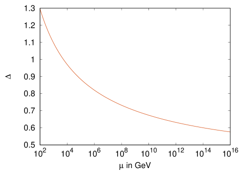
Figure 1: $\Delta$ plotted over the renormalisation scale. For energies above $10^{4}$ TeV, the three-loop terms have a bigger impact than the four-loop ones. Still, the four-loop contributions are at least half the size of the three-loop ones for the renormalisation scales under consideration.

Indeed, for renormalisation scales below $10^{4}$ GeV, the four-loop contributions have a larger impact than the three-loop ones. However, for larger scales, the accidental cancellation in the three-loop terms is lifted and the perturbative convergence improves.

3.3 A SUSY GUT example

Another useful application is to evolve the RGEs in the MSSM including right-handed neutrinos from a high scale down to $M_{Z}$, where it can be matched onto the SM. Such an example is given in the file numssm_example.cpp. To build the example call make numssm_example from the main folder. Let us assume the Yukawa and gauge couplings are set by some (unrealistically oversimplified) GUT scenario, i.e.

$$g_{1}=g_{2}=g_{3}=0.7,\qquad Y_{u}=Y_{\nu}=Y_{1}+Y_{2}\qquad Y_{d}=Y_{e}=Y_{1}-Y_{2},$$ (15)

with some numerical Yukawa matrices $Y_{1}$ and $Y_{2}$ and the right-handed neutrino mass matrix $M=10^{14}\cdot Y_{1}$, which gives rise to neutrino masses but does not influence the running of the gauge couplings and Yukawa matrices. These conditions hold at $M_{GUT}=2\times 10^{16}\ \mathrm{GeV}$.

The code numssm_example.cpp starts with defining the initial and final renormalisation scales

⬇

double MGUT = 2.e16;

double MZ = 91.1876;

The Yukawa matrices and the gauge couplings are defined by

⬇

yukawa zero, Y1, Y2;

gauge g;

Y1 << 1.e-4, 0., 0., 0., 2.e-2, 0., 0., 0., 0.4;

Y2 << 0., -2.e-3, 3.e-2, -2.e-3, 0., 0.5, 3.e-2, 0., 0.5;

g << 0.7, 0.7, 0.7;

Using those input parameters, and following Eq. (15) we construct a numssm object via

⬇

numssm values(g, Y1 + Y2, Y1 - Y2, Y1 - Y2, Y1 + Y2, zero, Y1*1.e14);

The matrix zero contains zeros in each entry and is used to set the Wilson coefficient of the Weinberg operator $\kappa$ to zero at the beginning.

Again, the ODEint stepper functions have to be set up for the numerical integration

⬇

using namespace boost::numeric::odeint;

typedef runge_kutta_fehlberg78< numssm, double, numssm, double, vector_space_algebra > stepper;

This time, however, we will use the rundown template which not only performs the integration but also determines the see-saw scale (i.e. the mass scales of the right-handed neutrinos) and integrates out the right-handed neutrinos at tree-level, when coming across these see-saw scales.

⬇

rundown<stepper,numssm,void> foo(values, log(MGUT), log(MZ));

Note, that although the name suggests otherwise, rundown works ‘both ways’, i.e. both from the high to the low as well as from the low to high renormalisation scale. Only when evolving to a lower renormalisation scale, however, it will check for thresholds and integrate out the relevant particles using the integrate_out() routine of the respective model (numssm in this case).

Since the MSSM contains two Higgs doublets, also the ratio of their respective vevs, $\tan\beta=v_{2}/v_{1}$, has to be defined in order to calculate the fermion masses.

⬇

double tanb(60.);

As before the quark masses and their mixing can be extracted from the Yukawa matrices by

⬇

class ckm quarks(values.Yu, values.Yd);

quarks.calculate();

In the lepton sector we additionally need the mass matrix of the left-handed neutrinos which is calculated from the Wilson coefficient of the Weinberg operator $\kappa$.

⬇

yukawa ML = values.getML(tanb); // left-handed neutrino mass matrix

class pmns leptons(ML, values.Ye);

leptons.calculate();

The results can be written to the standard output similar to

⬇

std::cout << "up-type masses (GeV): " << quarks.get_upmasses(tanb).transpose() << std::endl;

The complete output should then look like

⬇

nuMSSM parameters at MZ:

gauge couplings: 0.45494 0.63045 1.1092

ckm parameters: 0.95698 0.058163 0.030761 3.1416

up-type masses (GeV): 0.6205 7.3594 170.36

down-type masses (GeV): 0.0053232 0.20148 2.2537

PMNS parameters: 1.5057 0.037873 0.0012002 3.1416

neutrino masses (eV): 0.00037949 0.01031 3.4087

charged lepton massess (GeV): 0.0025152 0.095236 1.3424

3.4 Adding additional Models

In this example we outline the necessary steps for implementing additional models. As an example, we implement the RGEs for the SM with an additional singlet scalar field $s$ such that the scalar sector of the theory takes the form

$$\mathcal{L}_{\mathrm{self}}=-\frac{\lambda_{1}}{4}(\phi^{\dagger}\phi)^{2}-\frac{\lambda_{2}}{2}(\phi^{\dagger}\phi)\ (s^{\dagger}s)-\frac{\lambda_{3}}{4}(s^{\dagger}s)^{2},$$ (16)

where additional couplings are forbidden by an ad-hoc $\mathbb{Z}_{2}$ symmetry. For reference of such models see e.g. [48, 49, 50].

Regarding the fermion sector, this model is identical to the SM, since the singlet couples neither to quarks nor leptons. Therefore, the RGEs for the Yukawa couplings are the same as in the SM at leading order. The same holds also for the gauge couplings. We only need to adapt the RGEs in the scalar sector, which can be obtained from the general results in [15, 25].

Let us start this example with the header file nsm.h in the models folder. The class definition of the nsm class is

⬇

class nsm : public base<3,3> {

public:

nsm() : base<3,3>() {};

nsm(const gauge<3> g_in, const std::complex<double> La1_in,

const std::complex<double> La2_in, const std::complex<double> La3_in,

const yukawa Yu_in, const yukawa Yd_in, const yukawa Ye_in)

: base<3,3>(g_in, Yu_in, Yd_in, Ye_in, 1)

{ La << La1_in, La2_in, La3_in; };

nsm(const base<3,3> &X) : base<3,3>(X) {};

// contains the RGEs

void operator()(const nsm &X, nsm &dX, const double);

};

The first line lets the nsm class inherit the properties of the base class specifying the number of gauge couplings (3) and the number of scalar couplings (also 3: $\lambda_{1}$, $\lambda_{2}$, $\lambda_{3}$). After the public statement three constructors are defined. The first one, setting all couplings to 0, is inherited from base. The second one allows one to construct an nsm object using three complex variables as input for $\lambda_{1}$, $\lambda_{2}$, $\lambda_{3}$ in addition to the Yukawa couplings, which are then stored in the vector of self-couplings La. In this example, we will only consider one-loop RGEs, thus the variable (nloops) is set to one. For the function void operator() only the type of the input parameters has been changed in comparison to sm.h.

After the class definition there is an additional piece of code copied from sm.h that defines a struct that returns the modulus of the largest coupling in the model. This code does not need to be changed as long as there are no additional Yukawa couplings. In that case it should be straightforward to include theses additional couplings in the calculation of the largest coupling.

Now we are ready to set up the actual RGEs in the file nsm.cpp. Again, for the gauge and Yukawa couplings we can simply copy the SM ones from from sm.cpp. The code that needs some further adjustments is marked with a comment reading NEW CODE. The RGEs for the scalar couplings read

⬇

self<3> La2 = X.La.cwiseAbs2();

dX.La[0] = loopfactor*((12.)*X.La[0]*Yd2Tr + (-24.)*Yd4Tr

+ (4.)*X.La[0]*Ye2Tr + (-8.)*Ye4Tr + (12.)*X.La[0]*Yu2Tr

+ (-24.)*Yu4Tr + (-9./5.)*X.La[0]*g2[0]

+ (-9.)*X.La[0]*g2[1] + (9./5.)*g2[0]*g2[1]

+ (27./50.)*g4[0] + (9./2.)*g4[1]

+ 6.*La2[0] + 6.*La2[1]);

dX.La[1] = loopfactor*( 4.*X.La[0]*X.La[1] + 4.*X.La[1]*X.La[2] );

dX.La[2] = loopfactor*( 6.*La2[2] + 6.*La2[1]);

The first line defines a convenient abbreviation for the modulus squared of the vector self-couplings La. The second assignment resembles the RGE for $\lambda_{1}$. The part that stems from the interactions with the SM particles is, of course, the same as in sm.cpp. But there is an additional term from diagrams where singlet scalars appear in the loops. The next two assignments contain the RGEs of $\lambda_{1}$ and $\lambda_{2}$. We further deleted all higher loop orders that appear in sm.cpp for the sake of transparency.

The application of this model is demonstrated in the nsm_example.cpp file which is an adapted version of sm_example.cpp. Upon compilation and running the command line prompt should look like

⬇

nSM parameters at 1000 GeV:

Higgs self-couplings: (0.65818637,0) (1.0515135,0) (0.19774487,0)

Note that the numbers are chosen arbitrarily for demonstration purposes.

4 Summary and Outlook

We present the C++ library RGE++ for solving RGEs in theories with multiple couplings numerically. This concerns in particular the Standard Model up to four loops, as well as two-Higgs-doublet models and the MSSM up to three loops. Furthermore, RGE++ supports models with right-handed neutrinos and provides routines for decoupling them from the evolution. We provide three examples showcasing the usage and discuss the implemented classes in detail. The source code and further examples is available from https://github.com/Herren/RGEpp. The template-based structure gives the user the flexibility to implement higher-order corrections or new models easily.

References

- [1] K. G. Chetyrkin, Johann H. Kühn and M. Steinhauser “RunDec: A Mathematica package for running and decoupling of the strong coupling and quark masses” In Comput. Phys. Commun. 133, 2000, pp. 43–65 DOI: 10.1016/S0010-4655(00)00155-7
- [2] Barbara Schmidt and Matthias Steinhauser “CRunDec: a C++ package for running and decoupling of the strong coupling and quark masses” In Comput. Phys. Commun. 183, 2012, pp. 1845–1848 DOI: 10.1016/j.cpc.2012.03.023
- [3] Florian Herren and Matthias Steinhauser “Version 3 of RunDec and CRunDec” In Comput. Phys. Commun. 224, 2018, pp. 333–345 DOI: 10.1016/j.cpc.2017.11.014
- [4] Stephen P. Martin and David G. Robertson “Standard model parameters in the tadpole-free pure scheme” In Phys. Rev. D100.7, 2019, pp. 073004 DOI: 10.1103/PhysRevD.100.073004
- [5] Bernd A. Kniehl, Andrey F. Pikelner and Oleg L. Veretin “mr: a C++ library for the matching and running of the Standard Model parameters” In Comput. Phys. Commun. 206, 2016, pp. 84–96 DOI: 10.1016/j.cpc.2016.04.017
- [6] Stefan Antusch, Jörn Kersten, Manfred Lindner, Michael Ratz and Michael Andreas Schmidt “Running neutrino mass parameters in see-saw scenarios” In JHEP 03, 2005, pp. 024 DOI: 10.1088/1126-6708/2005/03/024
- [7] B. C. Allanach “SOFTSUSY: a program for calculating supersymmetric spectra” In Comput. Phys. Commun. 143, 2002, pp. 305–331 DOI: 10.1016/S0010-4655(01)00460-X
- [8] Abdelhak Djouadi, Jean-Loic Kneur and Gilbert Moultaka “SuSpect: A Fortran code for the supersymmetric and Higgs particle spectrum in the MSSM” In Comput. Phys. Commun. 176, 2007, pp. 426–455 DOI: 10.1016/j.cpc.2006.11.009
- [9] Werner Porod “SPheno, a program for calculating supersymmetric spectra, SUSY particle decays and SUSY particle production at e+ e- colliders” In Comput. Phys. Commun. 153, 2003, pp. 275–315 DOI: 10.1016/S0010-4655(03)00222-4
- [10] W. Porod and F. Staub “SPheno 3.1: Extensions including flavour, CP-phases and models beyond the MSSM” In Comput. Phys. Commun. 183, 2012, pp. 2458–2469 DOI: 10.1016/j.cpc.2012.05.021
- [11] Peter Athron, Jae-hyeon Park, Dominik Stöckinger and Alexander Voigt “FlexibleSUSY—A spectrum generator generator for supersymmetric models” In Comput. Phys. Commun. 190, 2015, pp. 139–172 DOI: 10.1016/j.cpc.2014.12.020
- [12] Peter Athron, Markus Bach, Dylan Harries, Thomas Kwasnitza, Jae-hyeon Park, Dominik Stöckinger, Alexander Voigt and Jobst Ziebell “FlexibleSUSY 2.0: Extensions to investigate the phenomenology of SUSY and non-SUSY models” In Comput. Phys. Commun. 230, 2018, pp. 145–217 DOI: 10.1016/j.cpc.2018.04.016
- [13] Marie E. Machacek and Michael T. Vaughn “Two Loop Renormalization Group Equations in a General Quantum Field Theory. 1. Wave Function Renormalization” In Nucl. Phys. B222, 1983, pp. 83–103
- [14] Marie E. Machacek and Michael T. Vaughn “Two Loop Renormalization Group Equations in a General Quantum Field Theory. 2. Yukawa Couplings” In Nucl. Phys. B236, 1984, pp. 221–232
- [15] Marie E. Machacek and Michael T. Vaughn “Two Loop Renormalization Group Equations in a General Quantum Field Theory. 3. Scalar Quartic Couplings” In Nucl. Phys. B249, 1985, pp. 70–92
- [16] I. Jack and H. Osborn “Two Loop Background Field Calculations for Arbitrary Background Fields” In Nucl. Phys. B 207, 1982, pp. 474–504 DOI: 10.1016/0550-3213(82)90212-7
- [17] I. Jack and H. Osborn “General Two Loop Beta Functions for Gauge Theories With Arbitrary Scalar Fields” In J. Phys. A 16, 1983, pp. 1101 DOI: 10.1088/0305-4470/16/5/026
- [18] I. Jack and H. Osborn “General Background Field Calculations With Fermion Fields” In Nucl. Phys. B 249, 1985, pp. 472–506 DOI: 10.1016/0550-3213(85)90088-4
- [19] Ming-xing Luo, Hua-wen Wang and Yong Xiao “Two loop renormalization group equations in general gauge field theories” In Phys. Rev. D 67, 2003, pp. 065019 DOI: 10.1103/PhysRevD.67.065019
- [20] Lohan Sartore “General RGEs for dimensionful couplings in the scheme” In Phys. Rev. D 102.7, 2020, pp. 076002 DOI: 10.1103/PhysRevD.102.076002
- [21] Florian Staub “SARAH 4 : A tool for (not only SUSY) model builders” In Comput. Phys. Commun. 185, 2014, pp. 1773–1790 DOI: 10.1016/j.cpc.2014.02.018
- [22] Florian Lyonnet and Ingo Schienbein “PyR@TE 2: A Python tool for computing RGEs at two-loop” In Comput. Phys. Commun. 213, 2017, pp. 181–196 DOI: 10.1016/j.cpc.2016.12.003
- [23] Lohan Sartore and Ingo Schienbein “PyR@TE 3”, 2020 arXiv:2007.12700 [hep-ph]
- [24] Daniel F. Litim and Tom Steudtner “ARGES – Advanced Renormalisation Group Equation Simplifier”, 2020 arXiv:2012.12955 [hep-ph]
- [25] Colin Poole and Anders Eller Thomsen “Constraints on 3- and 4-loop -functions in a general four-dimensional Quantum Field Theory” In JHEP 09, 2019, pp. 055 DOI: 10.1007/JHEP09(2019)055
- [26] C. Poole and A. E. Thomsen “Weyl Consistency Conditions and ” In Phys. Rev. Lett. 123.4, 2019, pp. 041602 DOI: 10.1103/PhysRevLett.123.041602
- [27] Joshua Davies, Florian Herren, Colin Poole, Matthias Steinhauser and Anders Eller Thomsen “Gauge coupling beta functions to four-loop order in the Standard Model” In Phys. Rev. Lett. 124, 2020, pp. 071803 DOI: 10.1103/PhysRevLett.124.071803
- [28] Gaël Guennebaud and Benoît Jacob “Eigen v3”, 2010 URL: http://eigen.tuxfamily.org
- [29] K. Ahnert and M. Mulansky “Odeint - Solving Ordinary Differential Equations in C++” In AIP Conference Proceedings 1389, 2011, pp. 001
- [30] Luminita N. Mihaila, Jens Salomon and Matthias Steinhauser “Gauge Coupling Beta Functions in the Standard Model to Three Loops” In Phys. Rev. Lett. 108, 2012, pp. 151602 DOI: 10.1103/PhysRevLett.108.151602
- [31] Luminita N. Mihaila, Jens Salomon and Matthias Steinhauser “Renormalization constants and beta functions for the gauge couplings of the Standard Model to three-loop order” In Phys. Rev. D86, 2012, pp. 096008 DOI: 10.1103/PhysRevD.86.096008
- [32] A. V. Bednyakov, A. F. Pikelner and V. N. Velizhanin “Anomalous dimensions of gauge fields and gauge coupling beta-functions in the Standard Model at three loops” In JHEP 01, 2013, pp. 017 DOI: 10.1007/JHEP01(2013)017
- [33] K. G. Chetyrkin and M. F. Zoller “Three-loop -functions for top-Yukawa and the Higgs self-interaction in the Standard Model” In JHEP 06, 2012, pp. 033 DOI: 10.1007/JHEP06(2012)033
- [34] A. V. Bednyakov, A. F. Pikelner and V. N. Velizhanin “Yukawa coupling beta-functions in the Standard Model at three loops” In Phys. Lett. B722, 2013, pp. 336–340 DOI: 10.1016/j.physletb.2013.04.038
- [35] A. V. Bednyakov, A. F. Pikelner and V. N. Velizhanin “Three-loop SM beta-functions for matrix Yukawa couplings” In Phys. Lett. B737, 2014, pp. 129–134 DOI: 10.1016/j.physletb.2014.08.049
- [36] Florian Herren, Luminita Mihaila and Matthias Steinhauser “Gauge and Yukawa coupling beta functions of two-Higgs-doublet models to three-loop order” In Phys. Rev. D97.1, 2018, pp. 015016 DOI: 10.1103/PhysRevD.97.015016
- [37] K. G. Chetyrkin and M. F. Zoller “-function for the Higgs self-interaction in the Standard Model at three-loop level” [Erratum: JHEP09,155(2013)] In JHEP 04, 2013, pp. 091 DOI: 10.1007/JHEP04(2013)091, 10.1007/JHEP09(2013)155
- [38] A. V. Bednyakov, A. F. Pikelner and V. N. Velizhanin “Higgs self-coupling beta-function in the Standard Model at three loops” In Nucl. Phys. B875, 2013, pp. 552–565 DOI: 10.1016/j.nuclphysb.2013.07.015
- [39] A. V. Bednyakov, A. F. Pikelner and V. N. Velizhanin “Three-loop Higgs self-coupling beta-function in the Standard Model with complex Yukawa matrices” In Nucl. Phys. B879, 2014, pp. 256–267 DOI: 10.1016/j.nuclphysb.2013.12.012
- [40] B. Grzadkowski and M. Lindner “Nonlinear Evolution of Yukawa Couplings” In Phys. Lett. B193, 1987, pp. 71
- [41] Debtosh Chowdhury and Otto Eberhardt “Global fits of the two-loop renormalized Two-Higgs-Doublet model with soft Z2 breaking” In JHEP 11, 2015, pp. 052 DOI: 10.1007/JHEP11(2015)052
- [42] Stephen P. Martin and Michael T. Vaughn “Two loop renormalization group equations for soft supersymmetry breaking couplings” [Erratum: Phys. Rev.D78,039903(2008)] In Phys. Rev. D50, 1994, pp. 2282 arXiv:hep-ph/9311340 [hep-ph]
- [43] P. M. Ferreira, I. Jack and D. R. T. Jones “The Three loop SSM beta functions” In Phys. Lett. B387, 1996, pp. 80–86 DOI: 10.1016/0370-2693(96)01005-2
- [44] B. Grzadkowski, M. Lindner and S. Theisen “Nonlinear Evolution of Yukawa Couplings in the Double Higgs and Supersymmetric Extensions of the Standard Model” In Phys. Lett. B198, 1987, pp. 64–68
- [45] Robert V. Harlander, Luminita Mihaila and Matthias Steinhauser “The SUSY-QCD beta function to three loops” In Eur. Phys. J. C63, 2009, pp. 383–390 DOI: 10.1140/epjc/s10052-009-1109-9
- [46] Thomas Deppisch, Stefan Schacht and Martin Spinrath “Confronting SUSY SO(10) with updated Lattice and Neutrino Data” In JHEP 01, 2019, pp. 005 arXiv:1811.02895 [hep-ph]
- [47] C. Patrignani “Review of Particle Physics” In Chin. Phys. C40.10, 2016, pp. 100001
- [48] Robert M. Schabinger and James D. Wells “A Minimal spontaneously broken hidden sector and its impact on Higgs boson physics at the large hadron collider” In Phys. Rev. D 72, 2005, pp. 093007 DOI: 10.1103/PhysRevD.72.093007
- [49] Brian Patt and Frank Wilczek “Higgs-field portal into hidden sectors”, 2006 arXiv:hep-ph/0605188
- [50] Matthew Bowen, Yanou Cui and James D. Wells “Narrow trans-TeV Higgs bosons and H hh decays: Two LHC search paths for a hidden sector Higgs boson” In JHEP 03, 2007, pp. 036 DOI: 10.1088/1126-6708/2007/03/036