Topological Obstructions in Neural Networks’ Learning

Abstract

We apply topological data analysis methods to loss functions to gain insights into learning of deep neural networks and deep neural networks’ generalization properties. We use the loss function’s Morse complex to relate the local behaviour of gradient descent trajectories with global properties of the loss surface. We define the neural network’s Topological Obstructions’ score (“TO-score”) with the help of robust topological invariants, barcodes of the loss function, that quantify the ”badness” of local minima for gradient-based optimization. We have made experiments for computing these invariants for fully-connected, convolutional and ResNet-like neural networks on different datasets: MNIST, Fashion MNIST, CIFAR10, CIFAR100 and SVHN. Our two principal observations are 1) the neural network’s barcode decreases with the increase of the neural network’s depth and width, thus the topological obstructions to learning diminish, 2) in certain situations there is an intriguing connection between the length of minima’s segments in the barcode and the minima’s generalization errors.

Introduction

Mathematically, if one opens the “black box” of deep learning, there are two immediate mysteries. Firstly, the algorithms based on gradient descent achieve almost zero loss with deep neural nets (DNN), although the loss functions of DNNs are nonconvex, have many saddles and multiple local minima. Secondly, DNNs have good generalization properties, namely, there is essentially no overfitting despite that the number of parameters in DNN is much bigger than the number of data points (Goodfellow et al., 2016; LeCun et al., 2015). To gain insights into these mysteries we propose to apply methods of topological data analysis to loss functions.

In this paper, we study the global properties of the loss function’s gradient flow. Our main tools, the topological data analysis of the loss function and the loss function’s Morse complex invariants, relate local behaviour along gradient trajectories to global properties of the loss surface.

1 Barcodes of loss functions

1.1 How to quantify badness of local minima.

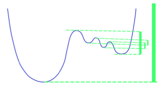
How to quantify to what extent a given local minimum represents an obstacle for gradient-based optimization trajectories? Clearly, some minima pose more obstacles than others (see Figure 1). Usually the badness of local minima is quantified via the Hessian. However this is often unsatisfactory. For example the two minima on Figure 1 pose different difficulties although locally they look the same.

Figure 1: The two local minima, indicated by circles, look the same locally, but pose different difficulty to gradient-based optimization. The difficulty is quantified by the lengths of the green segments (bars) $s_{p}$ attached to these minima in $\text{Barcode}\,(L)$

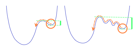
Barcodes are precisely the numerical invariants that quantify the badness of local minima, more specifically, the minima’s global, reparametrization invariant ”badness” characteristics.

To escape a vicinity of a given local minimum $p$, a path starting at $p$ has to climb up on the loss landscape. However, climbing up to the closest ridge point from which the path can then go down in the direction of another minimum, does not guarantee that such a path descends to a point with loss lower than $L(p)$. For any local minimum $p$ there is the minimal height ($L(p)$ plus “penalty”) to which a path starting at $p$ has to climb, before it can reach a point with loss lower than $L(p)$ (see Figure 1).

Definition. Consider various paths $\gamma:[0,1]\rightarrow\Theta$ starting from local minimum $p$ and going to a point with loss lower than $L(p)$. Let $m_{\gamma}\in\Theta$ be the maximum of the loss $L$ on such path $\gamma$. Let $h_{p}$ be the minimal value of $m_{\gamma}$, or the height corresponding to the smallest ”penalty” for going to lower loss points starting from $p$:

$$h_{p}=\min_{\begin{subarray}{c}\gamma:[0,1]\rightarrow\Theta\\ \gamma(0)=p,\,L(\gamma(1))<L(p)\end{subarray}}\max_{t}L\big{(}\gamma(t)\big{)}$$ (1)

We associate with the local minimum $p$ the segment $s_{p}=[L(p),h_{p}]$. The segment’s length represents the minimal obligatory penalty for reaching lower loss points starting from $p$.

Definition. The barcode of minima for loss function is the disjoint union of the segments $s_{p}$ for local minima $p$, plus half-line accounting for the global minimum

$$\text{Barcode}\,(L)=[L(p_{\text{global}}),+\infty)\sqcup\big{(}\sqcup_{p}[L(p),h_{p}]\big{)}$$ (2)

see Figure 9 for a simple example.

The bigger the length of the segment $s_{p}$ the more difficult for gradient-based optimization trajectory trapped in a vicinity of $p$ to escape it and to reach lower loss values.

Saddles of small indexes and flat regions in vicinity’s of them can also pose obstacles for gradient-based optimization (Dauphin et al., 2014). All these obstacles are topological in nature, as any critical point or critical manifold. We discuss in the appendix the analogous topological invariants, barcodes of arbitrary indices (Barannikov, 1994; Le Peutrec et al., 2013), quantifying ”lifetimes” of saddles.

1.2 Barcodes via gradient flow on segments. Algorithm

In terms of gradient flow the barcode of minima can be calculated using the formula (1) as follows.

Let $\gamma(t)$, $t\in[0,1]$ be a path from a local minimum $p$ to a lower value minimum $p^{\prime}$. Consider action of the gradient flow generated by the gradient vector field

$$\dot{\theta}=-\textrm{grad}\,L$$

on the path $\gamma$, up to the reparametrization of the path. At each path’s point $t$ the gradient $\textrm{grad}\,L$ is decomposed into sum

$$-\textrm{grad}\,L=(-\textrm{grad}\,L)_{\|}+(-\textrm{grad}\,L)_{n}$$

of two components, where $(-\textrm{grad}\,L)_{\|}$ is parallel to the tangent vector to $\gamma(t)$ and $(-\textrm{grad}\,L)_{n}$ is orthogonal to it. The action by the tangent component $-(\textrm{grad}\,l)_{\|}$ is absorbed into reparametrization of path $\gamma(t)$. The gradient flow moves the curve $\gamma(t)$ by $-(\textrm{grad}\,L)_{n}$, the normal component of $-\textrm{grad}\,L$.

In realization we optimize the path by applying the orthogonal gradient $-(\textrm{grad}\,L)_{n}$, multiplied by learning rate, to a set of points approximating $\gamma(t)$. The gradient is calculated via SGD or other gradient-based methods. The maximum value of the loss function on the set of points approximating $\gamma(t)$ decreases for sufficiently small learning rate at each iteration. For Lipshitz $L$ and sufficient number of points this also ensures that $\max_{t}L\left(\gamma\left(t\right)\right)$, the maximal value on the path, decreases. Details of this optimization on sampled paths are described in section 3.1.

After optimizing a set of sampled paths starting at the given minimum $p$ and going to points with lower loss, we calculate the segment corresponding to $p$ in $\text{Barcode}\,(L)$ using formula (1). This is summarized in Algorithm 1.

  $S_{\text{0}}\leftarrow\{\text{Minima (optimized sampled points)}\,p\in\Theta\}$

  $\text{Barcode}\leftarrow\varnothing$

  for $p\in S_{0}$ in increasing order of $L(p)$ do

     $b[p]\leftarrow L(p)$

     $h[p]\leftarrow+\infty$

     for ${(q\in S_{0})}\And{(L(q)<L(p))}$ do

        $\gamma\leftarrow\text{Optimized sampled path}\gamma(0)=p,\gamma(1)=q$

        $h[p]\leftarrow\min\left(h[p],\max_{t\in[0,1]}L(\gamma(t))\right)$

     end for

     $\text{Barcode}\leftarrow\text{Barcode}\sqcup\left[b[p],h[p]\right]$

  end forreturn Barcode

Algorithm 1 Barcode of minima computation for loss function of DNN.

This algorithm gives a stochastic estimate for $\text{Barcode}\,(L)$.

1.3 Topological obstructions (TO-) score

In the ideal situation, if the loss function has a single minimum and no other local minima, then all gradient trajectories $\dot{x}=-\textrm{grad}\,L$ for all starting points, except for a set of measure zero, always converge to the single minimum.

We define the neural network’s Topological obstructions (TO-) score as the distance between the minima’s barcode of the neural network’s loss function $L$ and the minima’s barcode of such ideal function $L^{\text{ideal}}$ with the single minimum at the same level as the value of the global minimum of $L$:

$$\textrm{TO Score}=\textrm{Distance}\left(\textrm{Barcode}\left(L\right),\textrm{Barcode}\left(L^{\textrm{ideal}}\right)\right)$$ (3)

The distance here is the standard Bottleneck distance (Efrat et al., 2001) on barcodes, also known as Wasserstein$-\infty$ distance $\mathbb{W}_{\infty}$:

$$\mathbb{W}_{\infty}(\mathcal{D},\mathcal{D}^{\prime}):=\inf_{\pi\in\Gamma(\mathcal{D},\mathcal{D}^{\prime})}\sup_{a\in\mathcal{D}\cup\Delta}\lVert a-\pi(a)\rVert.$$ (4)

Here the barcode is represented as point cloud of points $(L(p),h_{p})\in\mathbb{R}^{2}$ and the point $L(p_{\text{global}})\in\mathbb{R}$ on the line ”at infinity”, $\Delta$ denotes the ”diagonal” in $\mathbb{R}^{2}$ and $\Gamma(\mathcal{D},\mathcal{D}^{\prime})$ denotes the set of partial matchings between $\mathcal{D}$ and $\mathcal{D}^{\prime}$ defined as bijections between $\mathcal{D}\cup\Delta$ and $\mathcal{D}^{\prime}\cup\Delta$.

We have found in our experiments that the TO-score diminishes with increase of the network depth and width, see section 2, Figures 3 and 4.

1.4 Lifetimes of saddles, r-saddles’ barcode via gradient descent on simplexes

Here we describe analogous algorithm for estimation of barcodes for saddles of arbitrary index $r\geq 1$. These barcodes quantify the index $r$ saddles’ ”lifetimes”. The general definition of the higher barcodes is described in the Appendix. It is based on the evolution of higher dimensional topologial features in the sublevel sets of the loss. The $r-$th barcode records the ”birth” and ”death” intervals of $r-$dimensional topological features.

For the calculation of the higher barcodes one first optimizes sampled $(r+1)-$simplices. This is similar to the optimization of sampled $1-$simplices described in section 1.1. At each interior point of the simplex the gradient $\textrm{grad}\,L$ is decomposed again into the sum

$$-\textrm{grad}\,L=(-\textrm{grad}\,L)_{\|}+(-\textrm{grad}\,L)_{n}$$

of two components, where $(-\textrm{grad}\,L)_{\|}$ is parallel to the simplex’s tangent plane and $(-\textrm{grad}\,L)_{n}$ is orthogonal to it. The action by tangent component $-(\textrm{grad}\,l)_{\|}$ is absorbed into the reparametrization of the simplex. The gradient flow moves the simplex by $-(\textrm{grad}\,L)_{n}$, the normal component of $-\textrm{grad}\,L$.

The set of optimized simplices is constructed inductively starting from a set of optimized sampled $0$-simplices (minima), then optimized $1-$simplices for each pair of minima; then optimized $2-$simplex for every triple of sampled minima etc.

After optimizing the set of sampled simplices, we calculate the filtration on this set defined by the maximal value of loss on the given simplex. Next step is the construction of filtered simplicial complex from the optimized simplices. The linear boundary operator $\partial_{r}$ acts on the linear space formally generated by $(r+1)-$simplices by sending a simplex to the alternated sum of its $r-$faces. Next the filtration is used to calculate the “births” and the “deaths” of topological features, via bringing the set of the boundary linear operators $\partial_{r}$ to simple form (Barannikov, 1994; Zomorodian, 2001; Le Peutrec et al., 2013).

This calculation is summarized in the Algorithm 2.

  Require: $\text{B}(C,r)$: function computing “births”-“deaths” intervals of filtered complex $C$ in dimension $r$

  $S_{j}\leftarrow\{\text{optimized sampled }j\text{-simplices}\,\Delta\subset\Theta\},j\leq i$

  $F\leftarrow\text{filtration on }\cup_{j}S_{j}$ defined by $\max_{\Delta}L$

  $C\leftarrow$ simplicial complex $\cup_{j}S_{j}$ with filtration $F$

  for $r<i$ do

     $\text{Barcode}^{r}(L)\leftarrow\text{B}(C,r)$

  end forreturn $\text{Barcode}^{r}(L)$, for all $r<i$

Algorithm 2 Higher Barcodes computation.

The index $r$ TO-score for index $r$ barcodes is defined by the same formula (3), where $L^{ideal}$ is an ideal function without critical points except for the global minimum. Zero TO-scores for all indexes indicates that the loss function, after a change of parametrization in $\Theta$, can be made convex.

1.5 Zero TO-scores and convexity up to reparametrization.

Theorem. Let $L$ be a piece-wise smooth continuous function on a domain $D\subset\mathbb{R}^{n}$, $n\geq 5$, with $\nabla(L)|_{\partial D}$ pointing outside the domain $D$, and such that for all $r\geq 0$ index-$r$ TO-score$(L)=0$. Then there exist an arbitrary small smooth perturbation of $L$ which is convex after a smooth reparametrization of the domain $D$.

The idea of the proof, given in the appendix, is as follows. Firstly, take a small smooth perturbation $\tilde{L}$ of $L$ whose all critical points are nondegenerate. Then the vanishing of all TO-scores of $L$ implies that all $\tilde{L}$ critical points, except for the global minimum, come in pairs with small ”lifespans”. Then the standard elimination of pairs of critical points technique (Smale, 1967) shows the existence of a small perturbation $\hat{L}$ of $L$ whose only critical point is the non-degenerate global minimum. Lastly, a diffeomorphism making $\hat{L}$ convex is constructed with the help of the gradient flow of $\hat{L}$.

1.6 Barcode and optimal learning rates

The lengths of segments in the barcode are known to be equal to the Arrhenius law’s activation energies from the expressions for the exponentially small eigenvalues of the Witten Laplacian (Le Peutrec et al., 2013). These Witten Laplacian small eigenvalues were shown recently to play role in determining the optimal learning rates for stochastic gradient descent (Shi et al., 2020; Zhang et al., 2017). This gives yet another argument for the necessity of developing an accurate assessment for the lengths of segments in $\text{Barcode}(L)$ for neural networks.

1.7 Lowering of barcodes with the increase of neural networks’ depth and width

Embedding of Neural Networks. The neural networks which we consider can be embedded, preserving the loss, into similar networks, which are wider and/or deeper, and which have more parameters. For example, in the FCC case one can add an extra neuron in any layer and set all its incoming and outcoming weights to zero. Similar embeddings can be constructed with CNN architectures. These loss preserving embeddings permit to compare the barcodes of networks of similar type with different number of parameters.

An increase in the number of parameters leads to the lowering of the value of a given minimum, which gets a possibility to descent lower in new directions.

It turns out that in the considered networks the barcodes of minima also get lower. Examples of calculations of minima’s barcodes for bench optimization functions were given in (Barannikov et al., 2019), where this barcode’s lowering phenomena was confirmed for neural networks with few neurons.

We demonstrate the phenomena of barcodes’ lowering with the increase of network depth and width on the MNIST, FMNIST datasets with fully-connected neural networks with 2,3,4,6 and 8 hidden layers in section 2.1, and on CIFAR10 dataset in section 2.2 with convolutional neural networks CNN32-1,CNN32-2,CNN32-3, CNN64-1, CNN64-2, CNN128-1.

1.8 Complexity

Complexity of the proposed method is linear with respect to $n$, the number of points used for the approximation of each path. The gradient’s estimation at each point was calculated at each step during the paths’ optimization, requiring $O(Cn)$ operations, where $C$ is the number of weights in the neural network. The number of epochs in path’s optimization required for full convergence is typically the same as the number of epochs required for the optimization of minima.

1.9 Related work

Recently there were several applications of topology related ideas to neural networks e.g. (Kim et al., 2020; Moor et al., 2020), see (Chazal & Michel, 2017) for a review.

Two works studied optimization of curves and first showed that the local optima found by stochastic optimization methods are connected by curves with surprisingly flat training and test losses (Draxler et al., 2018; Garipov et al., 2018). The paper (Gotmare et al., 2018) established the wide generality of the mode connectivity framework. Further, the work (Fort & Jastrzebski, 2019) showed an existence of low loss subspaces connecting a set of minima. Also the work (Kuditipudi et al., 2019) gave an explanation of the minima connectivity, assuming generic properties of neural network such as dropout stability or noise stability of a network. The work (Skorokhodov & Burtsev, 2019; Czarnecki et al., 2019) demonstrates that the loss surface of neural networks conceals regions with arbitrary 2D landscape patterns, implicating its diversity and optimization complexity. The work (Zhao et al., 2020) has related the mode connectivity property with robustness against adversarial attacks.

As we have emphasized, a part of the set of maximal values on the almost “flat”, “mode-connecting” curves from these papers have, from our point of view, a specially distinguished meaning on equal footing with the values of loss at the minima. We demonstrate in section 2 that a portion of these maximal values on the optimized curves, after the combinatorial procedure, extracting the “penalty” values associated with each minimum, gives in certain situations a somewhat better prediction for minima’s generalization error.

We have also used the numerical invariants, that we extracted from the maximal values on the almost “flat” curves, in order to define a robust topological characteristic of the neural network, the TO-score. This gives a way for the application of a vast series of results on the stability of barcodes, see e.g. (Chazal & Michel, 2017), in the context of deep neural networks loss functions and architectures.

In the work (Li et al., 2018) a new technique for 2D visualization of neural networks’ loss surfaces was described. They concluded that most of the networks with residual connections have large convex areas and confirmed the “flat minima” hypothesis. The work (Choromanska et al., 2015) empirically verified that for large-size networks, most local minima are equivalent and yield similar performance on a test set and attempted to explain this property through the use of random matrix theory applied to the analysis of critical points in high degree polynomials on the sphere. The work (Nguyen, 2019) showed that every sublevel set of the loss function of a class of deep overparameterized neural nets with piecewise linear activation functions is connected and unbounded if “one of the hidden layers” is wide enough.

The properties of minima are also a topic of study. The well-known “flat minima” hypothesis (Hochreiter & Schmidhuber, 1997) states that flat minima generalize better. While confirmed by some studies (Keskar et al., 2016; Li et al., 2018) the network could be reparametrized to transform flat minima to sharp minima (Dinh et al., 2017). The work (He et al., 2019) concluded that at a local minimum there exist many asymmetric directions such that the loss increases abruptly along one side, and slowly along the opposite side – which they call “asymmetric valleys”.

2 Experiments on the lowering of barcodes

We show in this section how the barcodes are calculated by the proposed procedure (Algorithm 3, together with Algorithm 4 to tackle convergence problems for more complicated loss surfaces) and demonstrate the lowering of barcodes with increase of the neural networks depth.

2.1 Fully connected neural networks.

Figure 2: Barcodes of fully-connected deep neural networks (consisting of 2, 3, 4, 6, 8 layers) on MNIST and FMNIST datasets. The global minima correspond to infinite bars.

(a) MNIST

(b) FMNIST

Figure 3: The effect of decreasing TO score with the growth of number of layers in FC networks.

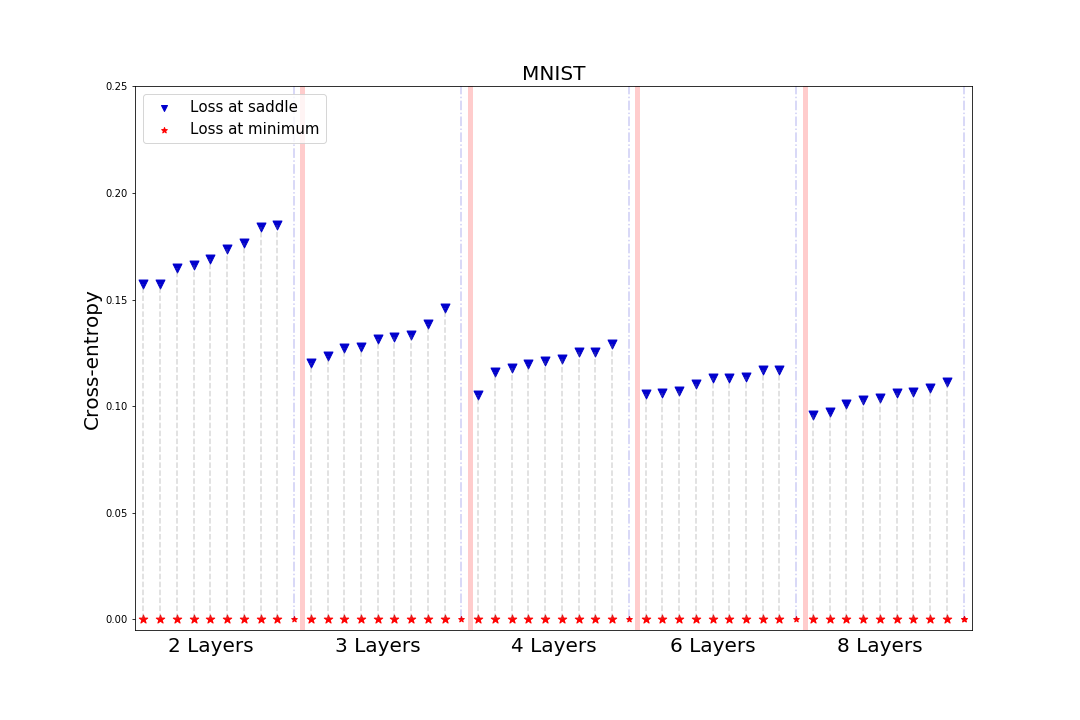
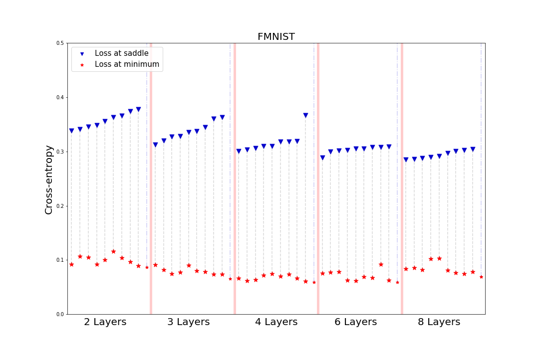
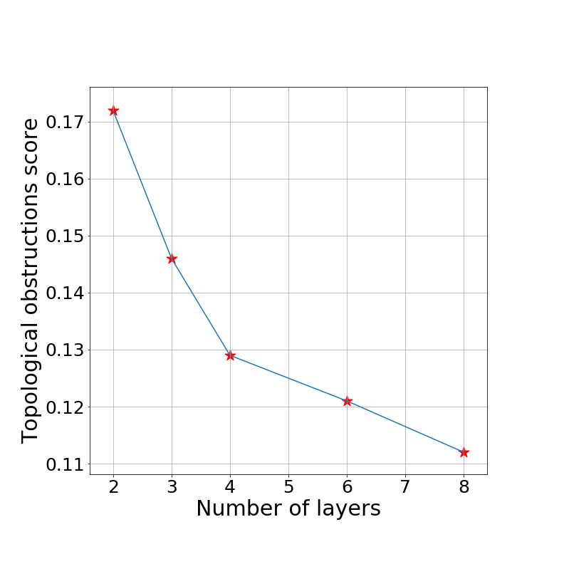
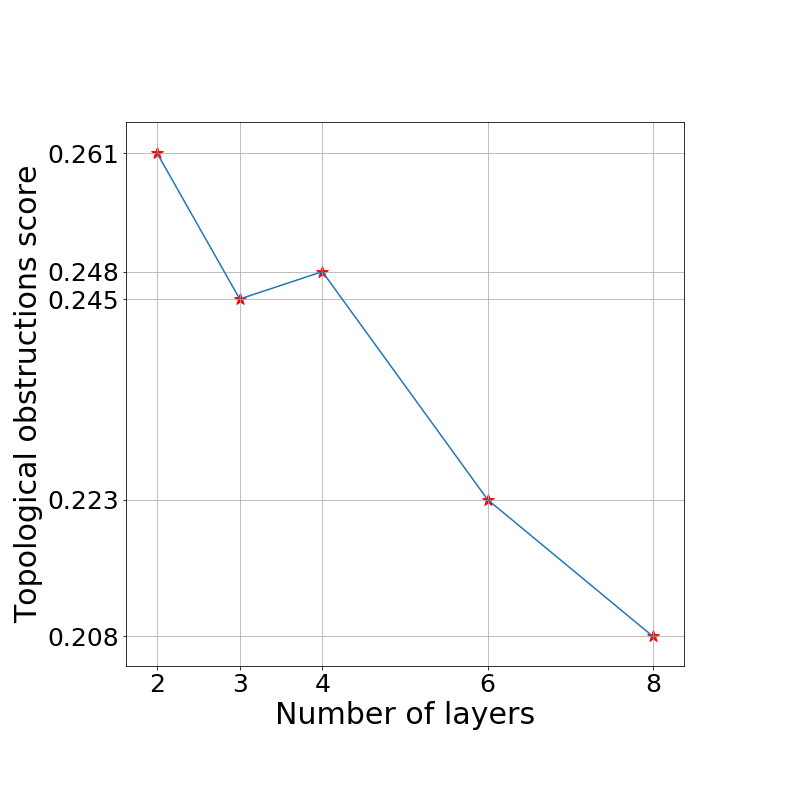
We demonstrate the lowering of barcodes on MNIST and FMNIST datasets using fully connected neural networks with 2,3,4,6 and 8 layers with 32 neurons in each layer, see Figure 2. We have randomly chosen a set of 10 minima trained until full convergence using Adam (Kingma & Ba, 2014) and Cyclical Learning Rate (Smith, 2015). Each pair of minima was connected by a path in the form of line segment. Then the training procedure described in section 1.2 was applied to the path. After the low loss connecting path is obtained, for each path the maximal value of loss is found, and then for each of minima $p$ the lowest value maximum $h_{p}$ on such paths is calculated. Then $[L(p),h_{p}]$ gives the segment corresponding to the given minimum in the barcode.

(a) Increase of number of channels in convolutional layer.

(b) Networks sorted by the numbers of parameters.

Figure 4: Barcodes for Convolutional Neural Networks. Effect of the increase of parameters’ number on the barcodes’ height for CNNs.

2.2 Convolutional neural networks (CNN).

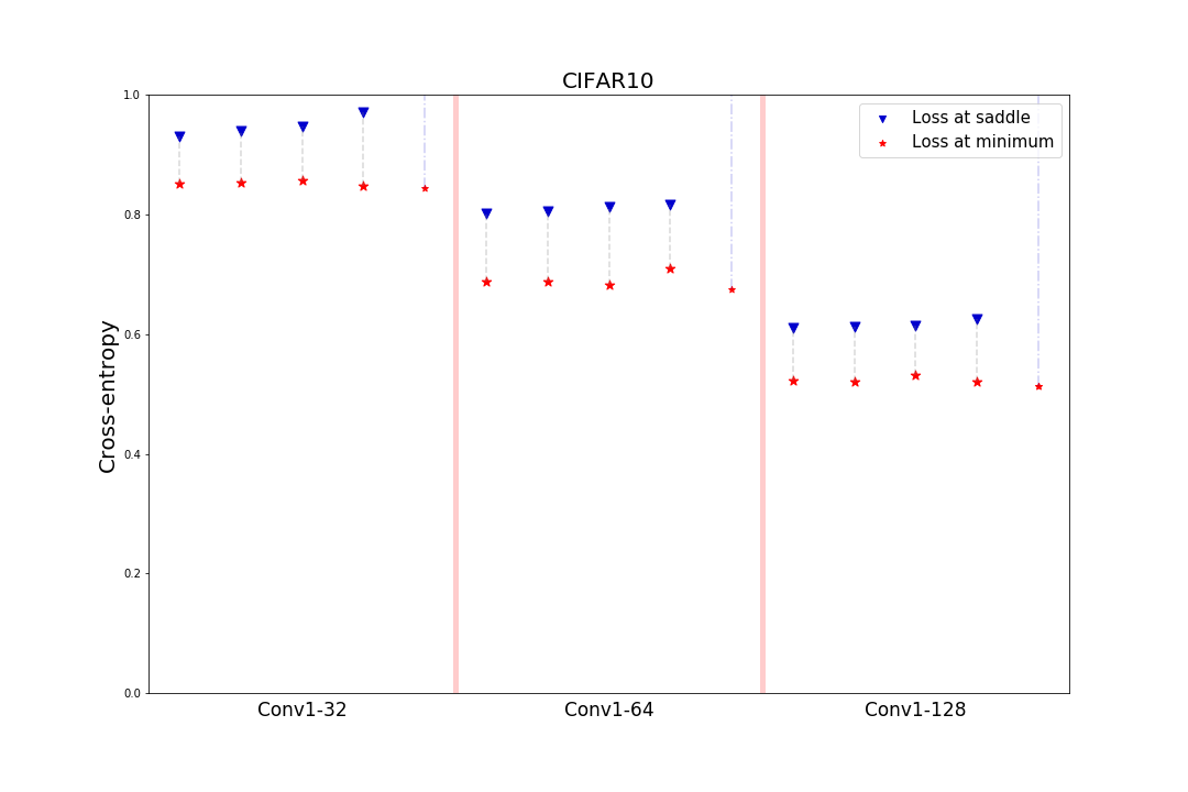
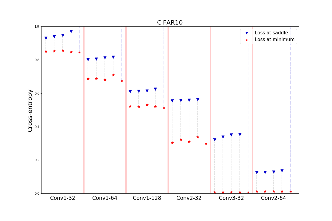
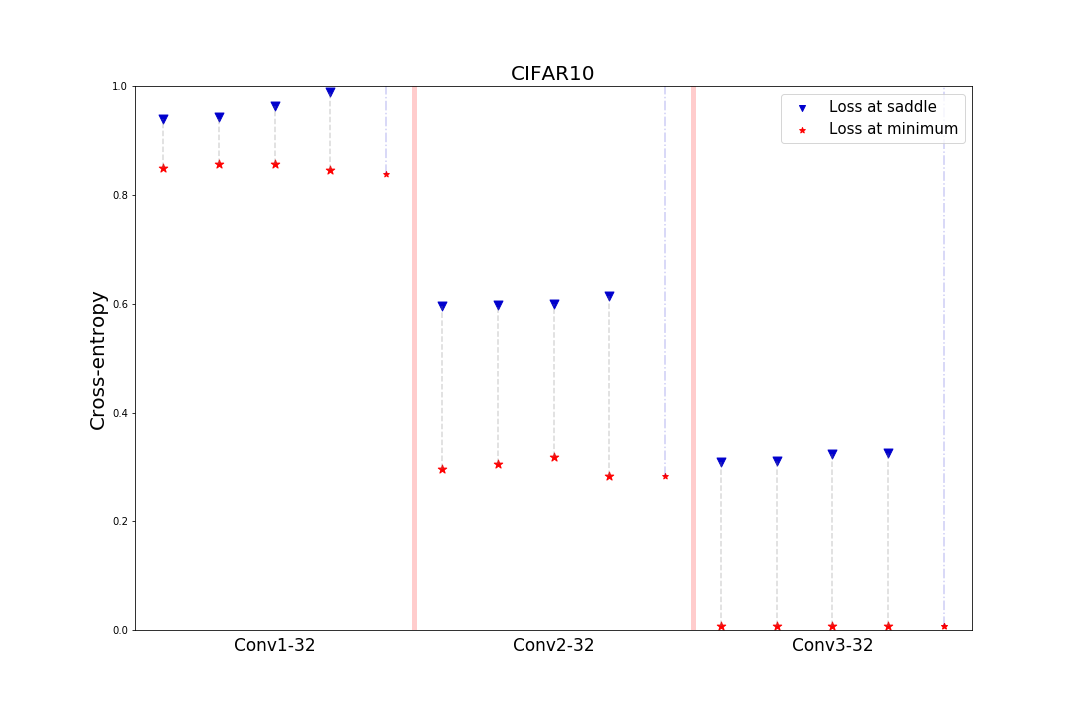
To validate the barcodes’ lowering hypothesis we have experimented with various CNN architectures on the well-known CIFAR10 dataset. For this purpose we have used standard networks, containing one, two and three convolutional layers, see Tables 8,9,10. The number of parameters in the last FC layer remains constant among CNNs with the same number of channels, to pay closer attention to the convolutional layers. As a downsampling method max-pooling operation was used to obtain the same spatial size before final FC layer for each network. The six convolutional networks from our experiments in this section have between 7K (Conv1-32) and 117K (Conv2-64) parameters.

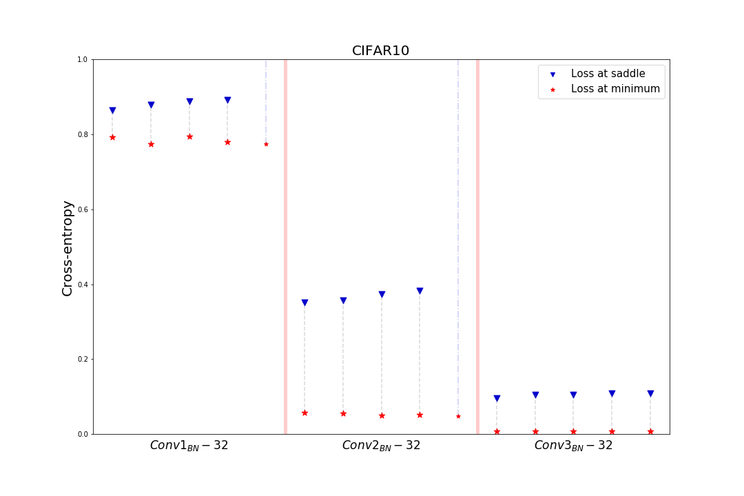
We have experimented also with CNN with Batch Normalization before activation function. As it was mentioned in prior works, Batch Normalization has a smoothing effect on the loss function. Figure 8 helps to evaluate this statement. We see that among CNNs of all considered depth, their counterparts with BN have both lower loss values in local minimas and in saddle points, which is especially clear in case of CNN-3. It can be understood from the position that initial points of the path, being initialized on a segment may have completely irrelevant parameters in early convolutional layers, inducing instability in activations which is later corrected by Batch Normalization.

Our experiments presented in the Figure 4 exhibit the barcode lowering phenomena. They show that the connection between the architecture of a network and the value of loss function at the saddle points $h_{p}$ associated with minima is established in a very intuitive way. Namely, these values are decreased both by increasing the number of convolutional layers or the number of channels in them. On Figure 4(a) we see monotonic decrease of loss function’s value in the found saddle points $h_{p}$ due to increase of channels number in a single convolutional layer. Moreover, on 4(b) one can distinguish even more rapid drop after adding new convolutional layers. Here we sort the architectures w.r.t. number of parameters and see the straightforward dependence. However, increasing the number of parameters in a simple architecture might lead to saturation of the considered effect.

3 ResNet’s barcodes and minima’s generalization property

Here we demonstrate that the height of segment from barcode is a topological characteristic of minima that is correlated with the generalization error of given minimum compared to minima obtained using other optimization parameters.

To investigate the connection between lengths of segments in the barcode and the generalization properties of obtained minima we have considered the work (Li et al., 2019).

In that paper, the designed experiment on CIFAR10 showed that neural networks trained with constant small learning rate have less test accuracy compared to ones trained with a higher learning rate, being annealed during the training process. The authors provide evidence that this is due to the effect of presence of easy-to-generalize, hard-to-fit patterns in the dataset, which are commonly learned initially with the small learning rate. On the other hand, when starting with a larger learning rate, these patterns are initially ignored and easy-to-fit, hard-to-generalize patterns attract at first a sufficient amount of attention. To explore this phenomenon from a different perspective, we have analyzed the loss surface global behaviour around both types of these minima.

Firstly, 8 ResNet-like (He et al., 2015) models were trained on CIFAR10 in two scenarios: using a constant small learning rate ($10^{-4}$) and applying annealing of learning rate (starting from $10^{-2}$ and ending with $10^{-4}$). The goal of the training process was to achieve the lowest possible loss on the training set. That’s why at that point we have obtained two groups of minima with similar, nearly zero values of loss function on the training set. However, their test accuracy differed significantly: 67.4% vs 75.7%, see Table 1. There is a huge generalization gap between the first types of minima compared to the second. Further training details can be found in the appendix.

3.1 Paths’ optimization for ResNet networks.

Initially minima were connected by straight segments on which we have selected points within equal distance between each other. Our experiments showed that for different types of model’s architectures and datasets the optimal number of points may vary. The most undesired behavior of path during the optimization process is when the number of points does not match the complexity of the model. It might lead to the situation when the optimized points converge to the local optima and reach low regions of loss function by the cost of becoming distant from each other. Due to the complexity of the loss surface, the structure of the path might be lost in that case.

Algorithm 3 Optimize path

Procedure proj($\theta_{i}$, $\theta_{j}$):

      return $\frac{\theta_{j}-\theta_{i}}{\|\theta_{j}-\theta_{i}\|}$

     

      Procedure STEP(path, $x$):

           $i\leftarrow 1$ while $i<|\text{\emph{path}}|-1$ do

                $\theta_{l}\leftarrow\text{path}_{i-1}$ $\theta_{c}\leftarrow\text{path}_{i}$ $\theta_{r}\leftarrow\text{path}_{i+1}$ $\nabla f_{\theta_{c}}=\nabla_{\theta_{c}}\big{(}\mathcal{L}(f_{\theta_{c}},x)\big{)}$ $\nabla^{left}f_{\theta_{c}}$ = $\langle\nabla f_{\theta_{c}},\text{proj}(\theta_{l},\theta_{c})\rangle\cdot\text{proj}(\theta_{l},\theta_{c})$ $\nabla^{right}f_{\theta_{c}}$ = $\langle\nabla f_{\theta_{c}},\text{proj}(\theta_{c},\theta_{r})\rangle\cdot\text{proj}(\theta_{c},\theta_{r})$ $\text{path}_{i}\leftarrow$ $\theta_{c}-\eta\big{(}\nabla f_{\theta_{c}}-\frac{\nabla^{left}f_{\theta_{c}}+\nabla^{right}f_{\theta_{c}}}{2}\big{)}$ $i\leftarrow i+1$

                end while

               

                return path

In our set up we have came up with a number of 19 points, connecting a pair of minima. Experimentally we observed that picking larger number does not give an improvement without a carefully tuned point insertion/rejection procedure. Also we discovered that $L_{2}$ regularization on parameters $\theta_{j}$ (single point belonging to the optimized path) has positive effect on optimization process as generally prevents points from moving far from the origin and as a result constrains pairwise distance. Every 25 epochs the decision was made via Algorithm 4 whether to insert new points preserving the structure of the path in it’s particular region or it is not necessary.

Procedure INSERTION(path, criterion):

      $\mu\leftarrow\frac{\|\theta_{last}-\theta_{first}\|_{2}}{|path|}$ $L_{max}\leftarrow max_{i}(L(\theta_{i})_{f,D})$ where $i\in[0,|path|-1]$ $T\leftarrow 1.2$, $i\leftarrow 0$, $B\leftarrow array()$, $D\leftarrow array()$ while $i<|path|-1$ do

           $D[i]\leftarrow criterion(\theta_{i},\theta_{i+1})$ $i:=i+1$

           end while

          if $max(D)>T$ then

                $max_{1}\leftarrow argmax_{i}(D)$ $max_{2}\leftarrow argmax_{j}(D\backslash\{max(D)\})$ $path[max_{1}]\leftarrow\frac{\theta_{max_{1}}+\theta_{max_{1}+1}}{2}$ $path[max_{2}]\leftarrow\frac{\theta_{max_{2}}+\theta_{max_{2}+1}}{2}$ Length $|path|\uparrow$ 2 $B\leftarrow path_{0}$ $path=path\backslash\{path_{0}\}$ $B\leftarrow path_{|path|}$ $path=path\backslash\{path_{|path|}\}$ Length $|path|\downarrow$ 2

                end if

               return $path,\,B$

               

               Procedure loss criterion($\theta_{i}$, $\theta_{i+1}$):

                     $loss=L((1-\alpha)\theta_{i}+\alpha\theta_{i+1})_{f,D}$, where $\alpha\in(0,1)$ return $\frac{max(loss)}{L_{max}}$

                    

                    Procedure distance criterion($\theta_{i}$, $\theta_{i+1}$):

                          return $\frac{\|\theta_{i}-\theta_{i+1}\|_{2}}{\mu}$

                         

Algorithm 4 Refine path

Insertion procedure is applied in combination with one of two proposed criterions, based on loss or distance between optimized points. To evaluate the values of the loss function between the optimized points on the path, the linear interpolation for the paths between them was used. Then a continuous set of values representing loss along path may be written as $\cup_{i=1}^{|path|}L(f,(1-\alpha)\theta_{i}+\alpha\theta_{i+1},D)$, where $\alpha\in[0,1]$. In case of loss criterion, the situation is clear, as revealing high values between optimized points our natural reaction is to insert additional point in that region to bypass the peak. However by doing that we may harm the structure of the path by producing superior density of points in a particular region of loss function. Our observations showed that frequently high loss between optimized points is a result of them becoming more distant from each other compared with other points, then we can set an upper bound on distance between them and, by adding intermediate points, maintain the structure of the path.

3.2 Barcode intervals’ length and generalization

The information about the obtained minima is summarized in Tables 1, 2 where the loss refers to the cross-entropy.

Type	Small LR	Annealing of LR
Train loss	0.009 $\pm 10^{-3}$	0.002 $\pm 10^{-4}$
Test loss	1.74 $\pm$ 0.058	1.32 $\pm$ 0.033
Train acc, %	99.97 $\pm$ 0.02	99.99 $\pm$ 0.01
Test acc, %	67.41 $\pm$ 0.93	75.74 $\pm$ 0.64

Table 1: CIFAR10 minima characteristics

Type	Small LR	Annealing of LR
Train loss	0.008 $\pm 10^{-3}$	0.001 $\pm 10^{-4}$
Test loss	0.53 $\pm$ 0.025	0.42 $\pm$ 0.015
Train acc, %	99.98 $\pm$ 0.01	99.99 $\pm$ 0.01
Test acc, %	88.12 $\pm$ 0.40	93.29 $\pm$ 0.19

Table 2: SVHN minima characteristics

(a) CIFAR10, test acc. (1): $67.41\pm 0.93$, (2): $75.74\pm 0.64$

(b) SVHN, test acc (1): $88.12\pm 0.40$, (2): $93.29\pm 0.19$

Figure 5: Differences of barcodes segments length for local minima trained with a constant small learning rate (left from the red line), and with annealing of learning rate (right from the red line). ResNet neural networks.

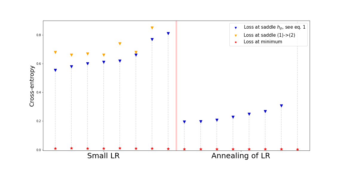
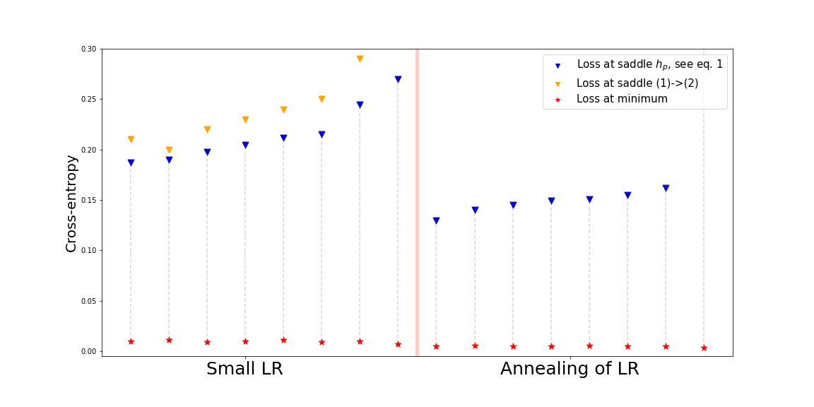
This experiment implied optimizing 28 paths between pairs of minima of type 1, 28 paths between pairs of type 2, and 64 paths from type 1 minima to type 2 minima. Considering the procedure described in section 1, barcodes were calculated based not only on the optimized points but also on intermediate points lying on the straight segments connecting the optimized points. To perform such evaluation, the following set of values $\alpha\in[0.2,0.4,0.6,0.8]$ was considered. We observe that loss at the saddle points for minima of the first type are always higher than for the second type minima. We have applied the same procedure for the SVHN dataset to validate this result and obtained the same outcome.

This tells us that even if models have nearly the same training loss, their generalization potential can be quantified by calculating barcodes and thus one can make a decision to use a model with a lower barcode as it indicates higher generalization guarantees. Though this process is very computationally costly and for now can not be effectively scaled across too complex architectures and large-scale-datasets.

In this experiment we have used the ResNet-like architecture with 195k trainable parameters, see Table 11.

4 Random points path optimization

In the cases of very high dimensional deep neural networks, the computation of $(-\textrm{grad}\,L)_{n}$ on sufficiently big number of points approximating a curve may become prohibitively expensive. Then, based on the recent works about DNN mode connectivity, e.g. (Garipov et al., 2018; Gotmare et al., 2018), we propose to change the curve optimization procedure, obtaining the following strategy: replace the computation of $(-\textrm{grad}\,L)_{n}$ for a large number of points on the curve by stochastic estimate via calculation on a fewer number of points distributed randomly along the curve. In this section, we show an example of running such algorithm on CIFAR100 dataset. We also use this approach to find optimized triangles and calculate the 1-saddle barcode using the algorithm 2, see Figure 6b.

Type	Value
Train loss	0.0072 $\pm$ 0.0007
Test loss	0.9093 $\pm$ 0.0130
Train acc, %	99.9812 $\pm$ 0.0060
Test acc, %	77.9280 $\pm$ 0.2665

Table 3: WideResNet16x10 CIFAR100 minima

First, 5 WideResNet16x10-like (Zagoruyko & Komodakis, 2016) models were independently trained on CIFAR100 dataset. Table 3 contains the characteristics of the learned minima. We used the WideResNet16x10 architecture containing about 17.1M of trainable parameters. Second, we optimize and evaluate a curve for each pair of the trained minima. We used a curve in the form of polygonal chain with one bend and fixed its endpoints during training. Finally, the barcode of the loss function was computed using the obtained minima and curves between them. Detailed training procedures for both minima and curves can be found in the Appendix.

Figure 6: Barcodes of WideResNet16x10 on CIFAR100 dataset. (a) Minima Barcode. (b) 1-saddle Barcode.

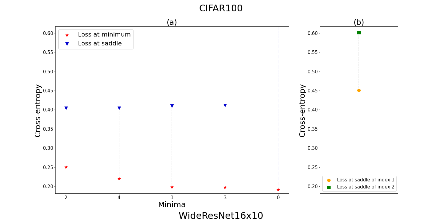
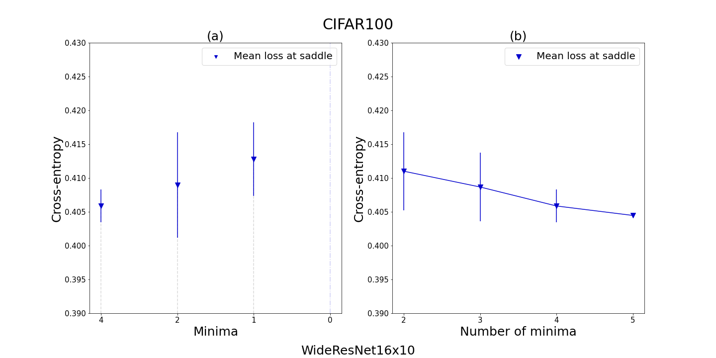
The resulting barcode is depicted in the Figure 6. From Figure 7, we also note that the barcode is a rather robust characteristic of the loss function in terms of both the set of learned minima and the number of minima used in the computation. In this experiment, the computation of the barcode requires an optimized curve between each pair of learned minima. Computational budget to train a curve was equivalent to the training budget for a minimum. Thus, this algorithm can be seen as an alternative approach for the barcode computation with better scalability.

Figure 7: Robustness of the barcode computation for WideResNet16x10 and CIFAR100 dataset. (a) Mean and standard deviation of minima’s saddles averaged over the choice of the minima’s set. (b) For the fixed minimum (minimum 4), dependence of the mean and standard deviation of the saddle in the barcode with increase of the minima’s set size and averaged over the choice of the minima’s set.

5 Conclusion

In this work we have described the topological invariants, Barcodes(L), and the neural networks’ Topological Obstruction’s score that provide the numerical characterization for “badness” of loss landscapes in gradient-based learning. The pattern of the barcodes diminishing and descending lower with increase of the neural network depth and width is found and confirmed on various datasets: MNIST, Fashion MNIST, CIFAR10. We have observed an intriguing connection between the lengths of segments in barcodes and the minima generalization ability.

Appendix

(a) Without Batch Normalization

(b) With Batch Normalization

Figure 8: Effect of Batch Normalization on the barcodes’ height for convolutional neural networks.

Appendix A Finding local minima

During networks training we used the following learning rate scheduler:

$$\begin{split}\begin{cases}lr^{max},&\mbox{if }b_{i}\leq|D|m_{1}\\ (1-\Delta_{i})\cdot lr^{max}+\Delta_{i}\cdot lr^{min},&\mbox{if }|D|m_{1}<b_{i}<|D|m_{2}\\ lr^{min},&\mbox{if }b_{i}\geq|D|m_{2}\end{cases}\end{split}$$

where $|D|$ - number of batches in the dataset and $\Delta_{i}=\frac{b_{i}-|D|m_{1}}{|D|(m_{2}-m_{1})}$. Without the loss of generality this system of conditions can be expressed as a function $S(m_{1},m_{2},lr^{max},lr^{min},i)$.

Note that in such a formulation $S(0,0,lr_{0},lr_{0},\cdot)$ will correspond to the simplest case, when the learning rate is fixed to the value $lr_{0}$ during the whole training process. Let’s denote it $S(lr_{0})$ for simplicity. In this work, we have used schedulers $S_{c10}:=S(10,80,10^{-2},10^{-4},\cdot)$ and $S_{svhn}:=S(50,100,5\cdot 10^{-2},10^{-4},\cdot)$ to observe the expected effect on CIFAR10 (Table 4) and SVHN (Table 5) datasets respectively in combination with Stochastic Gradient Descent and momentum $\nu=0.9$.

Type	Batch size	$\|\theta\|_{2}$	Scheduler	Epochs
1	256	0	$S(10^{-4})$	1500
2	256	0	$S_{c10}$	300

Table 4: CIFAR10 Training parameters.

Type	Batch size	$\|\theta\|_{2}$	Scheduler	Epochs
1	256	0	$S(10^{-4})$	1500
2	256	0	$S_{svhn}$	100

Table 5: SVHN Training parameters.

To train WideResNet16x10 on CIFAR100 dataset, we used the training procedure from the paper (Garipov et al., 2018), i.e., the following learning rate schedule together with hyperparameters from the Table 6:

$$\begin{split}\begin{cases}lr^{base},&\mbox{if }\alpha\leq 0.5\\ \left[1.0-\frac{(\alpha-0.5)}{0.4}\cdot 0.99\right]\cdot lr^{base},&\mbox{if }\alpha\leq 0.9\\ 0.01\cdot lr^{base},&\mbox{if }\alpha>0.9\end{cases}\end{split}$$

where $\alpha=\frac{m}{M}$ and $m$ is the number of the current epoch, $M$ - total number of epochs during training. We used Stochastic Gradient Descent and momentum $\nu=0.9$.

Batch size	$\|\theta\|_{2}$	$lr^{base}$	Epochs
128	$5\times 10^{-4}$	0.03	200

Table 6: WideResNet16x10 CIFAR100 Training hyperparameters.

To train LeNet-like model on FashionMNIST dataset, we used hyperparameters from the Table 7 and Stochastic Gradient Descent and momentum $\nu=0.9$.

Batch size	$\|\theta\|_{2}$	$lr^{base}$	Epochs
128	$10^{-3}$	0.01	50

Table 7: WideResNet16x10 CIFAR100 Training hyperparameters.

Figure 9: Barcode of a $1-\dim$ function.

Appendix B Architectures of NNs

CNN-1-C
$x^{0}$ = Conv(3, C, 5x5), ReLU
$x^{1}$ = MaxPooling(8x8)
$\hat{y}$ = Linear(16 $\cdot$ C, 10)

Table 8: Architecture of CNN-1-C used in the section 2 experiments.

CNN-2-C
$x^{0}$ = Conv(3, C, 5x5), ReLU
$x^{1}$ = MaxPooling(2x2)
$x^{2}$ = Conv(C, C, 5x5), ReLU
$x^{3}$ = MaxPooling(4x4)
$\hat{y}$ = Linear(16 $\cdot$ C, 10)

Table 9: Architecture of CNN-2-C used in the section 2 experiments.

CNN-3-C
$x^{0}$ = Conv(3, 32, 5x5), ReLU
$x^{1}$ = MaxPooling(2x2)
$x^{2}$ = Conv(32, 32, 5x5), ReLU
$x^{3}$ = MaxPooling(2x2)
$x^{4}$ = Conv(32, 32, 5x5), ReLU
$x^{5}$ = MaxPooling(2x2)
$\hat{y}$ = Linear(16 $\cdot$ 32, 10)

Table 10: Architecture of CNN-3-32 used in the section 2 experiments.

ResNet
$x^{0}$ = Conv(3, 16, 3x3), ReLU
$x^{1}$ = Conv(16, 16, 3x3), ReLU, Conv(16, 16, 3x3) + $x^{0}$
$x^{2}$ = MaxPooling(2x2), Conv(16, 32, 3x3), ReLU
$x^{3}$ = Conv(32, 32, 3x3), ReLU, Conv(32, 32, 3x3) + $x^{2}$
$x^{4}$ = MaxPooling(2x2), Conv(32, 64, 3x3), ReLU
$x^{5}$ = Conv(64, 64, 3x3), ReLU, Conv(64, 64, 3x3) + $x^{4}$
$x^{6}$ = MaxPooling(2x2), Conv(64, 64, 3x3), ReLU
$x^{7}$ = Conv(64, 64, 3x3), ReLU, Conv(64, 64, 3x3) + $x^{6}$
$x^{8}$ = MaxPooling(2x2), BatchNorm(64)
$\hat{y}$ = Linear($X^{8}$, 10)

Table 11: Architecture of Res-Net used.

LeNet
$x^{0}$ = Conv(1, 6, 5x5), ReLU, MaxPooling(2x2)
$x^{1}$ = Conv(6, 16, 5x5), ReLU, MaxPooling(2x2)
$x^{2}$ = Linear(256, 120), ReLU
$x^{3}$ = Linear(120, 84), ReLU
$x^{4}$ = Linear(84, 10)

Table 12: Architecture of LeNet used.

Appendix C Optimization of Path

While calculating barcodes for CIFAR10 the following hyperparameters were used in combination with Distance Criterion, responsible for efficiently preserving the structure of a path. In this work, we have used schedulers $S_{c10}^{o}:=S(270,300,2\cdot 10^{-3},1.25\cdot 10^{-4},\cdot)$ and $S_{svhn}^{o}:=S(170,200,2\cdot 10^{-3},1.25\cdot 10^{-4},\cdot)$ to observe the expected effect on CIFAR10 and SVHN datasets respectively in combination with Stochastic Gradient Descent and momentum $\nu=0$

While calculating barcode for WideResNet16x10 model and CIFAR100 dataset, we optimized the curves with the same training procedure as for the minima, i.e. see Appendix A.

Dataset	Batch size	$\|\theta\|_{2}$	Scheduler	Epochs
CIFAR10	150	$10^{-5}$	$S_{c10}^{o}$	300
SVHN	256	$10^{-5}$	$S_{svhn}^{o}$	200

Table 13: Path optimization hyperparameters.

Appendix D Visual interpretation of the insertion procedure

Figure 10: Illustration of point insertion.

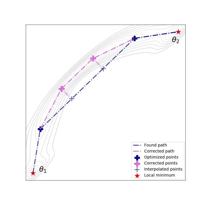
We motivate proposed insertion procedure with the following example on the model data. At the first stage, two points were optimized and they ended in reasonable regions of loss function with low loss values. However, it is visually noticeable that linear interpolation between them sometimes produce points completely off the desired manifold, preserving low values of loss function. But applying our procedure, by adding new points and optimizing them, they will reach relevant region and we can get rid of such negative effect, which can be viewed in Figure 10.

Appendix E Characteristics of an optimized path

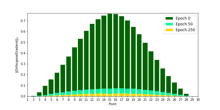
Norm of the gradient’s tangent projection in every point of a path, averaged across an epoch at different moments of the training. During training, we see a rapid drop in the middle.

Figure 11: Norm of tangent projection during optimization.

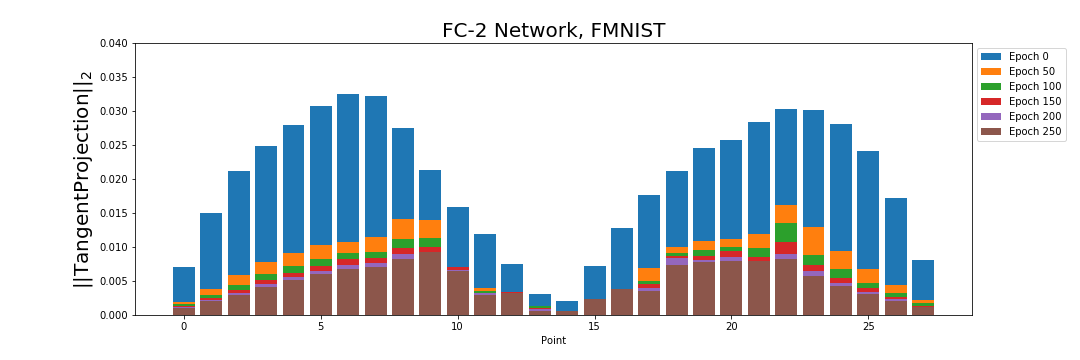
To illustrate the process of convergence of a single path, in each point, the norm of orthogonal gradient is accumulated after several epochs. We see that at the end of training the values are much lower and nearly zero, telling us that the points of obtained path nearly found flat regions of loss surface and will not change much after optimization.

Figure 12: Norm of orthogonal gradient during optimization.

Appendix F Morse complex and index $k$ critical points’ ”lifespans”

Morse theory principal notions are critical points and gradient flow trajectories. Gradient-based optimization algorithms’ two main objects are essentially parallel: minima and gradient descent trajectories.

Here for the sake of geometric intuitivity we describe the considered topological invariants under assumption that the loss is a generic smooth function.

Definition. A point $p$ is a critical point if the gradient at $p$ is zero: $df|_{p}=0$. A critical point $p$ is non-degenerate if the Hessian matrix of $f$ at $p$ is non-degenerate. The index of a non-degenerate critical point is the dimension of the Hessian’s negative subspace.

A gradient flow trajectory $x(t)$, $t\in[t_{0},+\infty)$ is a solution to

$$\dot{x}=-\nabla L(x)$$ (5)

A nondegenerate critical point of index $k$ is also called $k-$saddle. Near such point the function can be written in some coordinates as

$$L=-x_{1}^{2}\ldots-x_{k}^{2}+x_{k+1}^{2}\ldots+x_{n}^{2}.$$ (6)

Saddles of small index play important role in the gradient descent optimization algorithms. The gradient descent trajectories are attracted by such points, and more generally by critical manifolds of small index. Gradient trajectories spend long periods of time in vicinities of such points where the gradient is small, while they are trying to find one of the few descending, i.e. negative for the Hessian, directions.

The gradient flow trajectories can be extended back either to converge in the limit $t\to-\infty$ to a critical point, or to start from a point at the boundary of parameter domain. Here and further in this section we assume for simplicity that the gradient of $f$ at each point of the boundary of the domain $\Theta$ is pointing outside the domain, modifications for the general case are straightforward. For each point with nonzero gradient there is a unique gradient flow trajectory passing through this point. This gives a decomposition of the parameter domain.

The set of all points which lie on gradient flow trajectories converging to a given critical point in the limit $t\to-\infty$, is diffeomorphic to a ball of dimension $k$, where $k$ is the index of the critical point. Indeed, first notice that locally near the given critical point of index $k$ the set of such points lying on gradient flow trajectories emanating from this critical point is diffeomorphic to a ball of dimension $k$. Next this diffeomorphism can be extended to the set of all points lying on gradient flow trajectories emanating from this critical point, using the gradient flow. Similarly the union of all trajectories emanating from the boundary of the parameter domain is diffeomorphic to $S^{N-1}\times\mathbb{R}$.

Therefore, the parameter domain decomposes into pieces with uniform flow. For each critical point there is the cell formed by all gradient flow trajectories converging in the limit $t\to-\infty$ to this critical point.

Morse complex records how these cells are glued to each other to form the nontrivial part of the decomposition of the total parameter domain.

Let

$$\mathcal{M}(p_{\alpha},p_{\beta})=\bigg{\{}\gamma:\mathbb{R}\rightarrow M^{n}\big{|}\bigg{.}\\ \bigg{.}\dot{\gamma}=-(\textrm{grad}L)(\gamma(t)),\lim_{t\rightarrow-\infty}=p_{\alpha},\lim_{t\rightarrow+\infty}=p_{\beta}\bigg{\}}/\mathbb{R}$$

be the set of gradient trajectories connecting critical points $p_{\alpha}$ and $p_{\beta}$, where the natural action of $\mathbb{R}$ is by the shift $\gamma(t)\mapsto\gamma(t+\tau)$.

If $\textrm{index}(p_{\beta})=\textrm{index}(p_{\alpha})-1$ then generically the set $\mathcal{M}(p_{\alpha},p_{\beta})$ is finite. Let $\#\mathcal{M}(\left[p_{\alpha},\texttt{or}\right],\left[p_{\beta},\texttt{or}\right])$ denotes in this case the number of the trajectories, counted with signs taking into account a choice of orientation, between critical points $p_{\alpha}$ and $p_{\beta}$. Here we have fixed a choice of orientation ”or” of negative Hessian subspace at each critical point.

Let $\partial_{j}$ denotes the matrix with entries $\#\mathcal{M}(\left[p_{\alpha},\textrm{or}\right],\left[p_{\beta},\textrm{or}\right])$. Each critical points with a choice of orientation can be recorded as a vector (a generator) in vector space. Then $\partial_{j}$ is the linear operator

$$\partial_{j}\left[p_{\alpha},\texttt{or}\right]=\sum_{\textrm{index}(p_{\beta})=j-1}\left[p_{\beta},\texttt{or}\right]\#\mathcal{M}(p_{\alpha},p_{\beta})$$

An important property of matrices $\partial_{j}$ is that their consecutive composition is zero

$$\partial_{j}\circ\partial_{j-1}=0$$ (7)

This can be proved by looking at families of gradient flow trajectories connecting critical points with indexes $\textrm{index}(p_{\beta})=\textrm{index}(p_{\alpha})-2$. Generically such family is one-dimensional and compact, and therefore it is a disjoint union of circles and segments. The property 7 follows then from the fact that each segment has two boundary points, so that the corresponding composite gradient trajectories naturally cancel each other.

Such sets of matrices $\partial_{j}$ with the property (7) define a chain complex. Recall that a chain complex $(C_{*},\partial_{*})$ is a sequence of finite-dimensional vector spaces $C_{j}$ (spaces of ”$j-$chains”) and linear operators (”differentials”)

$$\rightarrow C_{j+1}\stackrel{{\scriptstyle\partial_{j+1}}}{{\rightarrow}}C_{j}\stackrel{{\scriptstyle\partial_{j}}}{{\rightarrow}}C_{j-1}\rightarrow\ldots\rightarrow C_{0},$$

which satisfy (7). The vector spaces in our case are $C_{j}=\mathbb{F}^{m_{j}}$ where $m_{j}$ is the number of index $j$ critical points and $\mathbb{F}$ is the field of coefficients which is most often taken in applications to be $\mathbb{F}=\{0,1\}$ or $\mathbb{Q}$. Chain complex can be thought of as the algebraic counterpart of intuitive idea of representing complicated geometric object as something decomposed into simple pieces.

The $j-$th homology of the chain complex $(C_{*},\partial_{*})$ is the quotient of vector spaces

$$H_{j}(C_{*},\partial_{*})=\ker\left(\partial_{j}\right)/\textrm{im}\left(\partial_{j+1}\right).$$ (8)

Elements from $\ker\left(\partial_{j}\right)$ are called ”cycles”.

For any pair of critical points $p_{\alpha}$, $p_{\beta}$ with $\mathcal{M}(p_{\alpha},p_{\beta})\neq\varnothing$, we have $L(p_{\alpha})>L(p_{\beta})$ since the value of the function is always decreasing along the gradient trajectory (5). Let $F_{r}C_{j}\subseteq C_{j}$ denotes the subspace of $C_{j}$ spanned by the critical points of index $j$ with critical value $L(p_{\alpha})\leq r$. It follows that:

$$\partial_{j}(F_{r}C_{j})\subset F_{r}C_{j-1}.$$ (9)

These subspaces $F_{r}C_{j}$ are nested: $F_{r_{1}}C_{j}\subseteq F_{r_{2}}C_{j}$ for any pair $r_{1}<r_{2}$.

The homology of the chain complex $(F_{r}C_{*},\partial_{*})$ are the homology of the subset $\Theta_{L\leq r}=\{L(x)\leq r|x\in\Theta\}$ of the parameter domain. In particular, the dimension of the $j-$th homology $H_{j}(F_{r}C_{*},\partial_{*})$ equals to the number of independent $j-$dimensional topological features in $\Theta_{L\leq r}$.

As $r$ increases the dimension of the homology $H_{*}(F_{r}C_{*},\partial_{*})$ can increase or decrease. These changes can only happen at $r$ equal to one of the critical values of the loss function. The ”Main” theorem on persistent homology, also sometimes called ”Structure” or ”Principal” theorem on persistent homology, (Barannikov, 1994, 2021; Zomorodian, 2001; Le Peutrec et al., 2013) describes these changes in terms of simple “birth”-”death” phenomena of cycles chosen uniformly across all values of $r$.

The relevant notion to formulate this result is the notion of filtration on the chain complex. The set of nested subspaces $(F_{r_{\alpha}}C_{*})$ indexed by a subset $\{r_{\alpha}\}\subset\mathbb{R}$ and satisfying (9) is called an ”$\mathbb{R}-$filtration”. Then the mentioned theorem can be described as the classification theorem for $\mathbb{R}-$filtered chain complexes.

It follows that the critical values of the loss function, except for the global minimum, are canonically split into pairs. Let us remark that this fact generalizes straightforwardly also to the case of critical manifolds and/or piece-wise smooth loss functions.

Such splitting implies in particular that each $k-$saddle of the loss function either kills a topological feature that was born at a lower $(k-1)-$saddle, or gives birth to a topological feature that is killed at a higher $(k+1)-$saddle. In both cases this gives the ”lifespan” bars from the barcode associated with these pairs of critical points. We expect that for critical points of small indexes these ”lifespan” bars from the higher barcodes are also located in a small lower part of the range of the loss values and the ”lifespans” of critical points of small indexes diminish with increase of the depth and the width of the deep neural networks.

Appendix G TO-score and convexity up to reparametrization

Theorem. Let $L$ be a piece-wise smooth continuous function on a domain $D\subset\mathbb{R}^{n}$, $n\geq 5$, with $-\nabla(L)|_{\partial D}$ pointing outside the domain $D$, and such that for all $r\geq 0$ index $r$ TO-score$(L)=0$. Then there exist an arbitrary small smooth perturbation of $L$ which is convex after a smooth reparametrization of the domain $D$.

Proof.

First, there exists an arbitrary small smooth perturbation $\tilde{L}$ of $L$ whose all critical points are nondegenerate by Stone-Weierstrass and Sard’s theorems. Then, because of stability of the barcode, see e.g. (Chazal & Michel, 2017), the vanishing of all TO-scores of $L$ implies that all $\tilde{L}$ critical points, except for the global minimum, come in pairs with small ”lifespans”. Then the first, the second and the third elimination theorems from (Milnor, 2015), see also (Smale, 1967), permit to eliminate all these pairs of critical points and the constructed perturbation is small because of the smallness of the critical ponts lifespans. This gives a smooth arbitrary small perturbation $\hat{L}$ of $L$ whose only critical point is the non-degenerate global minimum. A diffeomorphism making $\hat{L}$ convex is constructed then with the help of the $\hat{L}$ gradient flow. Namely the $\hat{L}$ gradient flow can be used to bring the domain $D$ to a neighborhood of the critical point, while rescaling the function, and by Morse lemma $\hat{L}$ is quadratic in some coordinates in a neighborhood of its unique critical point . ∎

Appendix H Error bars

Figure 13: Error bars in the expirement with FC deep neural networks with 2,3, and 4 hidden layers.

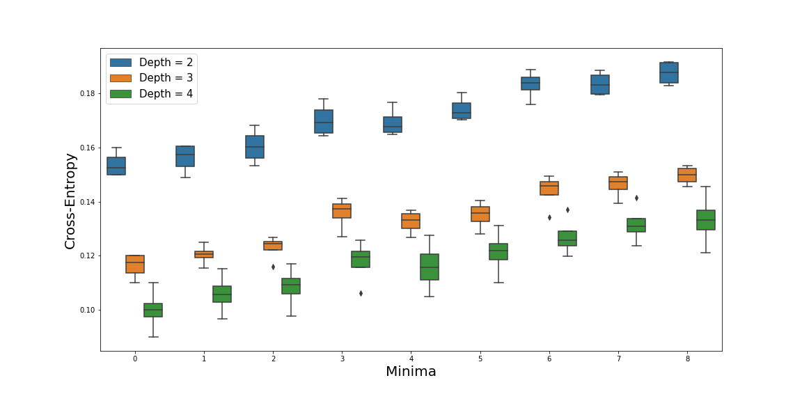
We report the error bars in the experiments with FC deep neural networks on Figure 13. Standard deviations are calculated for the values of the maxima of loss on the optimized curves connecting the minima.

Appendix I Higher Barcodes

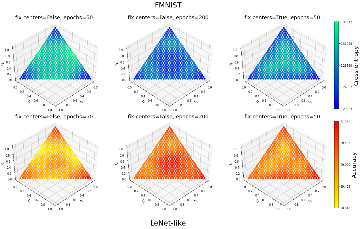
In this section we demonstrate some results on the computation of higher barcodes. Previously, we had a mapping from $[0,1]$-segment to a curve between two minima in the parameter space. Here we have a mapping from the standard triangle to a 2-dim simplex in the parameter space.

Figure 14: Standard 2-simplex.

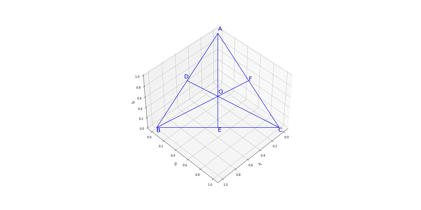
Consider a standard 2-simplex in $\mathbb{R}^{3}$, i.e. triangle, see Figure 14, and a point $t=(t_{1},t_{2},t_{3})$ inside this triangle. There are six possible orders of the coordinates $t_{1},t_{2},t_{3}$, each of which correspond to the case when this point $t=(t_{1},t_{2},t_{3})$ falls inside one of the smaller component triangles. Indeed,

$$\begin{gathered}\triangle AOD:t_{1}\leq t_{2}\leq t_{3},\quad\triangle AOF:t_{2}\leq t_{1}\leq t_{3},\\ \triangle BOD:t_{1}\leq t_{3}\leq t_{2},\quad\triangle BOE:t_{3}\leq t_{1}\leq t_{2},\\ \triangle COE:t_{3}\leq t_{2}\leq t_{1},\quad\triangle COF:t_{2}\leq t_{3}\leq t_{1}\end{gathered}$$ (10)

Assume $t=(t_{1},t_{2},t_{3})\in\triangle ABC$ and $t_{1}\leq t_{2}\leq t_{3}$. Then $t\in\triangle AOD$, and

$$\begin{gathered}D=\frac{1}{2}A+\frac{1}{2}B,\\ O=\frac{1}{3}A+\frac{1}{3}B+\frac{1}{3}C\end{gathered}$$ (11)

From this it follows:

$$\begin{gathered}B=2D-A,\\ C=3O-2D\end{gathered}$$ (12)

Finally, $t=t_{3}A+t_{2}B+t_{1}C=t_{3}A+t_{2}(2D-A)+t_{1}(3O-2D)=(t_{3}-t_{2})A+3t_{1}O+(2t_{2}-2t_{1})D$.

More generally, for every point $t=(t_{1},t_{2},t_{3})\in\triangle ABC$ with $t_{i}\leq t_{j}\leq t_{k}$, using the ordering of its coordinates we determine $t\in\triangle X_{1}OX_{2}$, where $X_{1}\in\{A,B,C\}$ and $X_{2}\in\{D,F,E\}$. Representation of $t$ as linear combination of vertices of the triangle $\triangle X_{1}OX_{2}$ is $t=(t_{k}-t_{j})X_{1}+3t_{i}O+(2t_{j}-2t_{i})X_{2}=\tilde{t_{1}}X_{1}+\tilde{t_{2}}O+\tilde{t_{3}}X_{2}$. Hence, every point $t$ inside the triangle $\triangle ABC$ falls into one of its component triangles and can be represented as linear combination of its vertices.

Type	Value
Train loss	0.1596 $\pm$ 0.0050
Test loss	0.2600 $\pm$ 0.0034
Train acc, %	94.3204 $\pm$ 0.2578
Test acc, %	90.7725 $\pm$ 0.2987

Table 14: LeNet FashionMNIST minima characteristics.

Similarly to one-dimensional case, we associated each of the points $A,B,C,D,F,E$ with a set of parameters of a DNN model. Our goal was to tune some of the parameters to obtain a ”triangle” of low loss and high accuracy. There were two ways we used to train this model. In the first one, we associated vertices of the triangle with the trained minima of a model and fixed them during training. In this case, there remained four sets (three - centers of triangle’s sides, one - center of the whole triangle) of trainable parameters which were tuned during training. In the second approach, we associated sides of the triangle with the trained curves of a model. Then six sets of parameters were fixed during training and one set is trainable.

The training algorithm was similar to the approach from (Garipov et al., 2018) used in Section 4. In this case, we sampled a point $t=(t_{1},t_{2},t_{3})\in\triangle ABC$. As explained before, we represented this point as linear combination of vertices $X_{1},O,X_{2}$ of a smaller triangle $\triangle X_{1}OX_{2}$ with new coefficients $\tilde{t_{1}},\tilde{t_{2}},\tilde{t_{3}}$. Finally, we computed a linear combination of parameter sets corresponding to $X_{1},O,X_{2}$ with new coefficients $\tilde{t_{1}},\tilde{t_{2}},\tilde{t_{3}}$.

Figure 15: Triangle model for WideResNet16x10 and CIFAR100 dataset, non-trainable sides’ centers.

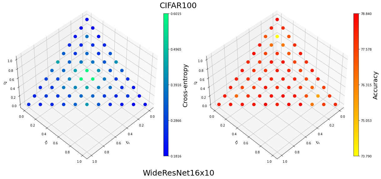
Figures 15, 16 show some examples of the observed results. In Figure 15, triangle model for WideResNet16x10 was trained on CIFAR100 with fixed sides’ centers. The training procedure was identical to training procedure for minima, i.e., see Appendix A. In Figure 16, we experimented with both regimes of work (fixed and trainable sides’ centers) and with different computational budgets for LeNet-like model and FashionMNIST dataset. Details on the minima’s training procedure are in Appendix A, Table 14. For the curve training we used the same training procedure as for the minima. Similarly for triangle training, only increasing the number of epochs for the trainable centers of the triangle’s sides. The more flexible model leads to better performance but requires bigger computational cost.

Figure 16: Triangle model for LeNet-like model and FashionMNIST dataset, trainable and non-trainable sides’ centers, different computational budgets.

In this case, barcode is a segment where the starting point is the maximum value of the triangle’s sides and the final point is the maximal value over the whole triangle. Figure 6 presents an example of the barcode computed for WideResNet16x10 and CIFAR100.

References

- Barannikov (1994) Barannikov, S. Framed Morse complexes and its invariants. Advances in Soviet Mathematics, 21:93–116, 1994. doi: 10.1090/advsov/021/03.
- Barannikov (2021) Barannikov, S. Canonical Forms = Persistence Diagrams. Tutorial. In European Workshop on Computational Geometry (EuroCG 2021), 2021.
- Barannikov et al. (2019) Barannikov, S., Korotin, A., Oganesyan, D., Emtsev, D., and Burnaev, E. Barcodes as summary of objective function’s topology. arXiv preprint arXiv:1912.00043, 2019.
- Chazal & Michel (2017) Chazal, F. and Michel, B. An introduction to topological data analysis: fundamental and practical aspects for data scientists. arXiv preprint arXiv:1710.04019, 2017.
- Choromanska et al. (2015) Choromanska, A., Henaff, M., Mathieu, M., Arous, G. B., and LeCun, Y. The loss surfaces of multilayer networks. In Artificial intelligence and statistics, pp. 192–204, 2015.
- Czarnecki et al. (2019) Czarnecki, W. M., Osindero, S., Pascanu, R., and Jaderberg, M. A deep neural network’s loss surface contains every low-dimensional pattern, 2019.
- Dauphin et al. (2014) Dauphin, Y. N., Pascanu, R., Gulcehre, C., Cho, K., Ganguli, S., and Bengio, Y. Identifying and attacking the saddle point problem in high-dimensional non-convex optimization. In Advances in Neural Information Processing Systems, pp. 2933–2941, 2014.
- Dinh et al. (2017) Dinh, L., Pascanu, R., Bengio, S., and Bengio, Y. Sharp minima can generalize for deep nets. arXiv preprint arXiv:1703.04933, 2017.
- Draxler et al. (2018) Draxler, F., Veschgini, K., Salmhofer, M., and Hamprecht, F. A. Essentially no barriers in neural network energy landscape. arXiv:1803.00885, 2018.
- Efrat et al. (2001) Efrat, A., Itai, A., and Katz, M. J. Geometry helps in bottleneck matching and related problems. Algorithmica, 31(1):1–28, 2001.
- Fort & Jastrzebski (2019) Fort, S. and Jastrzebski, S. Large scale structure of neural network loss landscapes. In Advances in Neural Information Processing Systems, pp. 6709–6717, 2019.
- Garipov et al. (2018) Garipov, T., Izmailov, P., Podoprikhin, D., Vetrov, D. P., and Wilson, A. G. Loss surfaces, mode connectivity, and fast ensembling of dnns. In Advances in Neural Information Processing Systems, pp. 8789–8798, 2018.
- Goodfellow et al. (2016) Goodfellow, I., Bengio, Y., Courville, A., and Bengio, Y. Deep learning, volume 1. MIT press Cambridge, 2016.
- Gotmare et al. (2018) Gotmare, A., Keskar, N. S., Xiong, C., and Socher, R. Using mode connectivity for loss landscape analysis. arXiv preprint arXiv:1806.06977, 2018.
- He et al. (2019) He, H., Huang, G., and Yuan, Y. Asymmetric valleys: Beyond sharp and flat local minima. In Advances in Neural Information Processing Systems, pp. 2553–2564, 2019.
- He et al. (2015) He, K., Zhang, X., Ren, S., and Sun, J. Deep residual learning for image recognition. arXiv:1512.03385, 2015.
- Hochreiter & Schmidhuber (1997) Hochreiter, S. and Schmidhuber, J. Flat minima. Neural Computation, 9(1):1–42, 1997.
- Keskar et al. (2016) Keskar, N. S., Mudigere, D., Nocedal, J., Smelyanskiy, M., and Tang, P. T. P. On large-batch training for deep learning: Generalization gap and sharp minima. arXiv preprint arXiv:1609.04836, 2016.
- Kim et al. (2020) Kim, K., Kim, J., Zaheer, M., Kim, J., Chazal, F., and Wasserman, L. Pllay: Efficient topological layer based on persistence landscapes. In 34th Conference on Neural Information Processing Systems (NeurIPS 2020), 2020.
- Kingma & Ba (2014) Kingma, D. P. and Ba, J. Adam: A method for stochastic optimization, 2014.
- Kuditipudi et al. (2019) Kuditipudi, R., Wang, X., Lee, H., Zhang, Y., Li, Z., Hu, W., Ge, R., and Arora, S. Explaining landscape connectivity of low-cost solutions for multilayer nets. In Advances in Neural Information Processing Systems, pp. 14601–14610, 2019.
- Le Peutrec et al. (2013) Le Peutrec, D., Nier, F., and Viterbo, C. Precise Arrhenius law for p-forms: The Witten Laplacian and Morse–Barannikov complex. Annales Henri Poincaré, 14(3):567–610, Apr 2013. ISSN 1424-0661. doi: 10.1007/s00023-012-0193-9.
- LeCun et al. (2015) LeCun, Y., Bengio, Y., and Hinton, G. Deep learning. nature, 521(7553):436–444, 2015.
- Li et al. (2018) Li, H., Xu, Z., Taylor, G., Studer, C., and Goldstein, T. Visualizing the loss landscape of neural nets. In Advances in Neural Information Processing Systems, pp. 6389–6399, 2018.
- Li et al. (2019) Li, Y., Wei, C., and Ma, T. Towards explaining the regularization effect of initial large learning rate in training neural networks. arXiv:1907.04595, 2019.
- Milnor (2015) Milnor, J. Lectures on the h-cobordism theorem. Princeton university press, 2015.
- Moor et al. (2020) Moor, M., Horn, M., Rieck, B., and Borgwardt, K. Topological autoencoders. In International Conference on Machine Learning, pp. 7045–7054. PMLR, 2020.
- Nguyen (2019) Nguyen, Q. On connected sublevel sets in deep learning. arXiv preprint arXiv:1901.07417, 2019.
- Shi et al. (2020) Shi, B., Su, W. J., and Jordan, M. I. On learning rates and Schrödinger operators. arXiv preprint arXiv:2004.06977, 2020.
- Skorokhodov & Burtsev (2019) Skorokhodov, I. and Burtsev, M. Loss landscape sightseeing with multi-point optimization. arXiv:1910.03867, 2019.
- Smale (1967) Smale, S. Differentiable dynamical systems. Bulletin of the American mathematical Society, 73(6):747–817, 1967.
- Smith (2015) Smith, L. N. Cyclical learning rates for training neural networks, 2015.
- Zagoruyko & Komodakis (2016) Zagoruyko, S. and Komodakis, N. Wide residual networks. In BMVC, 2016.
- Zhang et al. (2017) Zhang, Y., Liang, P., and Charikar, M. A hitting time analysis of stochastic gradient langevin dynamics. In Conference on Learning Theory, pp. 1980–2022. PMLR, 2017.
- Zhao et al. (2020) Zhao, P., Chen, P.-Y., Das, P., Ramamurthy, K. N., and Lin, X. Bridging mode connectivity in loss landscapes and adversarial robustness. arXiv preprint arXiv:2005.00060, 2020.
- Zomorodian (2001) Zomorodian, A. J. Computing and comprehending topology: Persistence and hierarchical Morse complexes (Ph.D.Thesis). University of Illinois at Urbana-Champaign, 2001.