Universal Adaptive Control of Nonlinear Systems

Abstract

This work develops a new direct adaptive control framework that extends the certainty equivalence principle to general nonlinear systems with unmatched model uncertainties. The approach adjusts the rate of adaptation online to eliminate the effects of parameter estimation transients on closed-loop stability. The method can be immediately combined with a previously designed or learned feedback policy if a corresponding model-parameterized Lyapunov function or contraction metric is known. Simulation results of various nonlinear systems with unmatched uncertainties demonstrates the approach.

I Introduction

Concurrent stabilization and model parameter estimation for uncertain nonlinear systems has long been a focus of the controls community. Despite several decades of research, a comprehensive direct adaptive control approach has remained elusive. The main difficulty in developing such a framework is the idea that the certainty equivalence principle cannot be employed when the model uncertainties are outside the span of the control input, i.e., are unmatched. Departure from certainty equivalence significantly complicates the design process as the controller must either anticipate or be robust to transients in the parameter estimates. This work will show that the certainty equivalence principle can be extended to systems with unmatched uncertainties by actively adjusting the rate of adaptation. The approach only requires the uncertainty be linearly parameterized and imposes no restrictions on the type or structure of the dynamics. Due to its generality, the approach is referred to as universal adaptive control.

Initial work in adaptive control of nonlinear systems used Lyapunov-like stability arguments and the certainty equivalence principle to construct stabilizing adaptive feedback policies for feedback linearized systems with matched uncertainties [1, 2, 3, 4, 5], i.e., those that can be directly canceled through control. The difficulty of extending these early approaches to general systems with unmatched uncertainties led to the development of adaptive backstepping [6, 7, 8, 9]. Restricting the system to have a triangular structure enabled the recursive application of the extended matching condition [10] and certainty equivalence. Combining a control Lyapunov function (clf) with parameter adaptation has also been investigated [10, 11] although these methods are often limited to systems with matched uncertainties. In [12], adaptive clf’s (aclf) were proposed for systems with unmatched uncertainties. However, computing an aclf is difficult because it entails stabilizing a modified system whose dynamics depend on its own clf. The above challenges spurred interest in indirect methods where an identifier is combined with an input-to-state stable (ISS) controller [10]. The strict ISS condition is needed as the identifier may not be fast enough to achieve closed-loop stability – an issue not encountered with direct methods as they employ Lyapunov-like arguments to derive the adaptation law. Recently, [13] used random basis functions [14, 15] to approximate unmatched uncertainties as matched but can require extensive parameter tuning as the underlying physics are not exploited.

The main contribution of this work is a new direct adaptive control framework based on certainty equivalence design for general nonlinear systems with unmatched uncertainties. The approach is comprised of two core ideas. The first is defining the unmatched control Lyapunov function which is a family of clf’s parameterized over all possible models. This follows the certainty equivalence philosophy of computing “infinitely-many” stabilizing clf’s instead of just one for all models. The second is to adjust the adaptation rate online to eliminate the effects of estimation transients on closed-loop stability. These ideas are further extended by introducing unmatched control contraction metrics, building upon [16], where a differential [17, 18] rather than explicit clf is utilized. The approach only requires the system be stabilizable or contracting for every parametric variation – an intuitive criteria easily included in algorithms that compute a clf or contraction metric. It can also be immediately combined with analytic or learned controllers with a known model-parameterized clf or contraction metric. Simulations illustrate the generality and effectiveness of the approach.

Notation: Symmetric positive-definite $n\times n$ matrices are denoted as $\mathcal{S}^{n}_{+}$. Positive and strictly-positive scalars are designated as $\mathbb{R}_{+}$ and $\mathbb{R}_{>0}$ respectively. The shorthand notation of a function $T$ parameterized by a vector $a$ with vector argument $s$ is $T_{a}(s):=T(s;a)$. The directional derivative of a smooth matrix $M:\mathbb{R}^{n}\times\mathbb{R}\rightarrow\mathcal{S}^{n}_{+}$ along a vector field $v:\mathbb{R}^{n}\times\mathbb{R}\rightarrow\mathbb{R}^{n}$ is $\partial_{v}M(x,t)=\sum_{i}^{n}\partial M/\partial x_{i}\,{v}_{i}(x,t)$. A desired trajectory and control input pair is $(x_{d},\,u_{d})$.

II Problem Formulation

This work addresses control of uncertain dynamical systems of the form

$$\dot{x}=f(x,t)-\Delta(x,t)^{\top}\theta+B(x,t)u,$$ (1)

with state $x\in\mathbb{R}^{n}$, control input $u\in\mathbb{R}^{m}$, nominal dynamics $f:\mathbb{R}^{n}\times\mathbb{R}\rightarrow\mathbb{R}^{n}$, and control input matrix $B:\mathbb{R}^{n}\times\mathbb{R}\rightarrow\mathbb{R}^{n\times m}$ with columns $b_{i}(x,t)$ for $i=1,\dots,m$. The uncertain dynamics are a linear combinations of known regression vectors $\Delta:\mathbb{R}^{n}\times\mathbb{R}\rightarrow\mathbb{R}^{p\times n}$ with rows $\varphi_{i}(x,t)$ for $i=1,\dots,p$ and unknown parameters $\theta\in\mathbb{R}^{p}$. We assume the dynamics Equation 1 are locally Lipschitz uniformly and the state $x$ is measurable. Systems with non-parametric or nonlinearly parameterized uncertainties can be converted into a linear weighting of handpicked or learned basis functions. A a new adaptive control framework based on certainty equivalence is developed for nonlinear systems in the form of Equation 1.

III Universal Adaptive Control

III-A Overview

This section presents the main technical results of this letter. First, a new type of clf is defined and an equivalence to stabilizability is established. The new clf is then used to adaptively stabilize Equation 1 using the certainty equivalence principle and online adjustment of the adaptation rate. The result is then extended to contracting systems where a new control contraction metric is defined.

III-B Unmatched Control Lyapunov Functions

Definition 1.

A smooth, positive-definite function $V_{\theta}:\mathbb{R}^{n}\times\mathbb{R}^{p}\times\mathbb{R}\rightarrow\mathbb{R}_{+}$ is an unmatched control Lyapunov function (uclf) if it is radially unbounded in $x$ and for each $\theta\in\mathbb{R}^{p}$

$$\underset{u\in\mathbb{R}^{m}}{\mathrm{inf}}\left\{\frac{\partial V_{\theta}}{\partial t}+\frac{\partial V_{\theta}}{\partial x}\left[f-\Delta^{\top}\theta+Bu\right]\right\}\leq-Q_{\theta}(x,t)$$

where $Q_{\theta}:\mathbb{R}^{n}\times\mathbb{R}^{p}\times\mathbb{R}\rightarrow\mathbb{R}_{+}$ is continuously differentiable, radially unbounded in $x$, and positive-definite with $Q_{\theta}(x,t)=0\iff x\neq x_{d}$.

Proposition 1.

The system Equation 1 is stabilizable for each $\theta\in\mathbb{R}^{p}$ if and only if there exists an uclf.

Proof.

“$\Leftarrow$”: Follows from [19, 20].
“$\Rightarrow$”: If Equation 1 is stabilizable for each $\theta\in\mathbb{R}^{p}$, then there exists a controller $u$ and a clf $V_{\theta}(x,t)$ [19] which, without loss of generality, satisfies $\dot{V}_{\theta}(x,t)\leq-Q_{\theta}(x,t)\leq 0$ where $Q_{\theta}(x,t)$ is a uniformly positive-definition function. Then, by Definition 1 $V_{\theta}(x,t)$ must be an uclf. ∎

Proposition 1 highlights the fundamental difference between an uclf and aclf (Definition 3, see Appendix): existence of an uclf is equivalent to the stabilizability of Equation 1 for each $\theta\in\mathbb{R}^{p}$. This equivalence means known approaches that compute a clf can be trivially extended to construct an uclf by searching over $x$ and $\theta$. Conversely, existence of an aclf is equivalent to Equation 1 being adaptively stabilizable [12]; a property not easily verified as it entails finding either 1) a stabilizing controller and adaptation law or 2) a stabilizing policy for a modified system that depends on its own (unknown) clf. As shown next, uclf’s play a central role in adaptive control of systems with unmatched uncertainties.

Theorem 1.

Consider an uncertain system of the form Equation 1. If an uclf $V_{\theta}(x,t)$ exists, then, for any strictly-increasing and uniformly-positive scalar function $\upsilon(\rho)$, the closed-loop system is globally asymptotically stable with the unmatched adaptation law

$$\dot{\hat{\theta}} =-\upsilon(\rho)\Gamma\Delta(x,t)\frac{\partial V_{\hat{\theta}}}{\partial{x}}^{\top},$$ (2a)

$$\dot{\rho} =-\frac{\upsilon(\rho)}{\upsilon_{\rho}(\rho)}\sum_{i=1}^{p}\frac{1}{V_{\hat{\theta}}(x,t)+\eta}\frac{\partial V_{\hat{\theta}}}{\partial\hat{\theta}_{i}}\dot{\hat{\theta}}_{i},$$ (2b)

where $\Gamma\in\mathcal{S}^{p}_{+}$, $\eta\in\mathbb{R}_{>0}$, and $\upsilon_{\rho}(\rho):={\partial\upsilon}/{\partial\rho}$.

Proof.

Consider the Lyapunov-like function

$$V_{c}(t)=\upsilon(\rho)(V_{\hat{\theta}}(x,t)+\eta)+\tfrac{1}{2}\tilde{\theta}^{\top}\Gamma^{-1}\tilde{\theta},$$

where $0<\eta<\infty$, and $\tilde{\theta}:=\hat{\theta}-\theta$. Differentiating $V_{c}(t)$,

$$\dot{V}_{c}(t) =\upsilon(\rho)\dot{V}_{\hat{\theta}}(x,t)+\dot{\rho}\upsilon_{\rho}(\rho)(V_{\hat{\theta}}(x,t)+\eta)+\tilde{\theta}^{\top}\Gamma^{-1}\dot{\hat{\theta}}$$

$$=\upsilon(\rho)\left\{\frac{\partial V}{\partial t}+\frac{\partial V_{\hat{\theta}}}{\partial x}\left[f-\Delta^{\top}\hat{\theta}+Bu\right]\right\}$$

$$\hphantom{=}+\upsilon(\rho)\frac{\partial V_{\hat{\theta}}}{\partial x}\Delta(x,t)^{\top}\tilde{\theta}+\upsilon(\rho)\sum_{i=1}^{p}\frac{\partial V_{\hat{\theta}}}{\partial\hat{\theta}_{i}}\dot{\hat{\theta}}_{i}$$

$$\hphantom{=}+\dot{\rho}\upsilon_{\rho}(\rho)(V_{\hat{\theta}}(x,t)+\eta)+\tilde{\theta}^{\top}\Gamma^{-1}\dot{\hat{\theta}},$$

where $\upsilon_{\rho}(\rho)=\partial\upsilon/\partial\rho$. Employing the certainty equivalence property in conjunction with Definition 1 and (2) yields $\,\dot{V}_{c}(t)\leq-\upsilon(\rho)Q_{\hat{\theta}}(x,t)\leq 0\,$ which implies that both $\,\upsilon(\rho)(V_{\hat{\theta}}(x,t)+\eta)\,$ and $\,\tilde{\theta}\,$ are bounded. Since $\,V_{\hat{\theta}}(x,t)>0\,$ for all $\,x\neq x_{d}\,$ and $\,\upsilon(\rho)>0$ uniformly, then both $\,V_{\hat{\theta}}(x,t)\,$ and $\,\upsilon(\rho)\,$ are bounded for all $\,x\neq x_{d}$. Since $\,\smash{\dot{\hat{\theta}}}=0\,$ when $x=x_{d}$, then from Equation 2b $\,\dot{\rho}=0\,$ so $\,\upsilon(\rho)\,$ remains bounded. Hence, $\,V_{\hat{\theta}}(x,t)\,$ is bounded because $\,\eta$, $\,\upsilon(\rho)$, and $\,\upsilon(\rho)(V_{\hat{\theta}}(x,t)+\eta)\,$ are bounded. Differentiating $\,\upsilon(\rho)Q_{\hat{\theta}}(x,t)\,$ and utilizing Equation 2b,

$$\frac{d}{dt}\left(\upsilon(\rho)Q_{\hat{\theta}}(x,t)\right)= ~{}\upsilon(\rho)\sum_{i}^{p}\left[\frac{\partial Q_{\hat{\theta}}}{\partial\hat{\theta}_{i}}-\frac{Q_{\hat{\theta}}(x,t)}{V_{\hat{\theta}}(x,t)+\eta}\frac{\partial V_{\hat{\theta}}}{\partial\hat{\theta}_{i}}\right]\dot{\hat{\theta}}_{i}$$

$$+\upsilon(\rho)\frac{\partial Q_{\hat{\theta}}}{\partial x}\dot{x}+\upsilon(\rho)\frac{\partial Q}{\partial t},$$

which is bounded by continuity of $\,V_{\hat{\theta}}(x,t),~{}Q_{\hat{\theta}}(x,t)\,$ and boundedness of $x$ and $\upsilon(\rho)$. Hence, $\upsilon(\rho)Q_{\hat{\theta}}(x,t)\,$ is uniformly continuous. Integrating $\dot{V}_{c}(t)$ yields $\int\limits_{0}^{\infty}\upsilon(\rho(\tau))Q_{\hat{\theta}}(x(\tau),\tau)d\tau\leq V_{c}(0)<\infty$, so by Barbalat’s lemma [21] $\,\upsilon(\rho)Q_{\hat{\theta}}(x,t)\rightarrow 0$. Since $\,\upsilon(\rho)>0\,$ uniformly and $\,Q_{\hat{\theta}}(x,t)=0\iff x=x_{d}\,$ then $\,x\rightarrow x_{d}\,$ as $t\rightarrow+\infty$. ∎

Remark 1.

Theorem 1 immediately extends to the case when $\sqrt{Q_{\theta}(x,t)}$ is an input to a virtual contracting system [17, 22] with $x$ and $x_{d}$ as particular solutions, rather than satisfying $Q_{\theta}(x,t)=0\Longleftrightarrow x=x_{d}$. As in [23], this follows from the hierarchical combination property of contracting systems, which generalizes the notion of a sliding variable [21].

Remark 2.

If the unknown parameters belong to a closed convex set $\Theta$, i.e., $\theta\in\Theta\subset\mathbb{R}^{p}$, then one can employ the projection operator $\mathrm{Proj}_{\Theta}(\cdot)$ to ensure $\hat{\theta}\in\Theta$ without affecting stability [21, 24].

Remark 3.

If an uclf is designed to use full desired trajectory for feedback, then an adaptive reference model – where $(x_{d},\,u_{d})$ is re-computed for every new parameter estimate $\hat{\theta}$ – is required for closed-loop stability. The origin of adaptive reference models will be discussed further in Section III-C.

Theorem 1 shows how the certainty equivalence property can be extended to systems with unmatched uncertainties by combining uclf with an effective adaptation gain $\upsilon(\rho)\Gamma$ that adjusts in response to whether the parameter adaptation transients terms are stabilizing or destabilizing in $\dot{V}_{c}(t)$. Inspecting Equation 2b, if the parameter adaptation transients is destabilizing then $\upsilon(\rho)\Gamma$ decreases thereby slowing the rate of parameter adaptation; the opposite occurs when the adaptation transients is stabilizing. Note the effective adaptation gain can be kept constant in this scenario, i.e., set $\dot{\rho}=0$, without affecting stability. This is advantageous given the well-known negative effects of high-rate adaptation.

Sufficiency for Theorem 1 requires the existence of an uclf, which is guaranteed if Equation 1 is stabilizable for each $\theta$ (Proposition 1). Practically, methods like backstepping, feedback linearization, or sum-of-squares (SOS) optimization can be utilized to compute $V_{\theta}(x,t)$ analytically while more recent data-driven approaches [25, 26] can also be used. For linear systems one can solve a parameter-dependent algebraic Ricatti equation. The above approaches find an explicit state transformation $z_{\theta}=T_{\theta}(x)$ where $V_{\theta}(x)=\tfrac{1}{2}z_{\theta}(x)^{\top}z_{\theta}(x)$ is a suitable uclf. Section III-C will show how the unmatched adaptation law Equation 2 can be combined with contraction theory to instead use a differential transformation $\delta_{z}=\mathcal{T}_{\theta}(x,t)\delta_{x}$ yielding a more general result.

III-C Unmatched Control Contraction Metrics

Contraction analysis [17] uses differential geometry to construct stabilizing feedback controllers without constructing an explicit state transformation. This is achieved by deriving a differential controller $\delta_{u}$ for the nominal differential dynamics of Equation 1 given by $\dot{\delta}_{x}=A(x,u,t)\delta_{x}+B(x,t)\delta_{u}$ where $A(x,u,t):=\partial f/\partial x+\sum^{m}_{i}\partial b_{i}/\partial x\,u_{i}$. Convex constructive conditions can be formulated for the so-called control contraction metric [18] $\ M:\mathbb{R}^{n}\times\mathbb{R}\rightarrow\mathcal{S}^{n}_{+}$ that ensures the distance defined by the metric $M$ between any two points, such as the current and desired state, converges exponentially with rate $\lambda$. More precisely, for a smooth manifold $\mathcal{M}$ and geodesic $\gamma:\left[0~{}1\right]\times\mathbb{R}\rightarrow\mathcal{M}$ with boundary conditions $\gamma(0,t)=x_{d}(t)$ and $\gamma(1,t)=x(t)$, the Riemannian energy $E(x,t):=\int_{0}^{1}\gamma_{s}(s,t)M(\gamma,t)\gamma_{s}(s,t)ds$ where $\gamma_{s}(s,t):=\partial\gamma/\partial s$ satisfies $\dot{E}(x,t)\leq-2\lambda E(x,t)$ yielding $x\rightarrow x_{d}$ exponentially with rate $\lambda$. In order to leverage the versatility of contraction, a new contraction metric suitable for adaptive control with unmatched uncertainties is required.

Definition 2.

A uniformly bounded Riemannian metric $M_{\theta}:\mathbb{R}^{n}\times\mathbb{R}^{p}\times\mathbb{R}\rightarrow\mathcal{S}^{n}_{+}$ is an unmatched control contraction metric (uccm) if, for each $\theta\in\mathbb{R}^{p}$, the dual metric $W_{\theta}(x,t):=M_{\theta}(x,t)^{-1}$ satisfies

$$B_{\perp}^{\top}\left(W_{\theta}A_{\theta}^{\top}+A_{\theta}W_{\theta}-\dot{W}_{\theta}+2\lambda W_{\theta}\right)B_{\perp}\preceq 0$$ (C1)

$$\partial_{b_{i}}W_{\theta}-W_{\theta}\frac{\partial b_{i}}{\partial x}^{\top}-\frac{\partial b_{i}}{\partial x}W_{\theta}=0,~{}~{}i=1,\dots,m$$ (C2)

where $A_{\theta}(x,u,t):=\partial f/\partial x-\sum^{p}_{i}\partial\varphi_{i}/\partial x\,\theta_{i}+\sum^{m}_{i}\partial b_{i}/\partial x\,u_{i}$, $B_{\perp}(x,t)$ is the annihilator matrix of $B(x,t)$, i.e., $B_{\perp}^{\top}B=0$, and $\dot{W}_{\theta}:=\partial W_{\theta}/\partial t+\partial_{\dot{x}}W_{\theta}$.

Remark 4.

The existence of uccm is equivalency to Equation 1 be contracting for each $\theta\in\mathbb{R}^{p}$; a criteria easily included in numerical methods that search for ccm’s. The proof can be found in Appendix.

Remark 5.

Since the proposed approach employs the the certainty equivalence principle, $\dot{W}_{\theta}$ does not include a parameter adaptation term which makes computing uccm tractable.

Remark 6.

If the uncertainty is matched then the metric does not need to depend on the unknown parameters [16].

An important property of uccm’s is summarized in Lemma 1; it will be later used in Theorem 2.

Lemma 1.

If an uccm $M_{\theta}(x,t)$ exists, then the Riemannian energy satisfies $\dot{E}_{\theta}(x,t)\leq-2\lambda E_{\theta}(x,t)$ for each $\theta\in\mathbb{R}^{p}$.

Theorem 2.

Consider an uncertain system of the form Equation 1. If an uccm $M_{\theta}(x,t)$ exists, then, for any strictly-increasing and uniformly-positive scalar function $\upsilon(\rho)$, the closed-loop system is globally asymptotically stable with the unmatched adaptation law

$$\dot{\hat{\theta}} =-\upsilon(\rho)\Gamma\Delta(x,t)M_{\hat{\theta}}(x,t)\gamma_{s}(1,t),$$ (3a)

$$\dot{\rho} =-\frac{\upsilon(\rho)}{\upsilon_{\rho}(\rho)}\sum_{i=1}^{p}\frac{1}{E_{\hat{\theta}}(x,t)+\eta}\frac{\partial E_{\hat{\theta}}}{\partial\hat{\theta}_{i}}\dot{\hat{\theta}}_{i},$$ (3b)

where $\Gamma\in\mathcal{S}^{p}_{+}$, $\gamma_{s}:={\partial\gamma}/{\partial s}$ is the geodesic speed, $\eta\in\mathbb{R}_{>0}$, and $\upsilon_{\rho}(\rho):={\partial\upsilon}/{\partial\rho}$.

Theorem 2 shows how the results of Section III-B can be extended to contracting systems where only a differential transform $\delta_{z}=\mathcal{T}_{\theta}(x,t)\delta_{x}$ is possible. As mentioned previously, the origin of adaptive reference models, i.e., where the desired trajectory $(x_{d},\,u_{d})$ are re-computed with $\hat{\theta}$, is more obvious under the lens of contraction. Taking the first variation of the Riemannian energy with Equation 1 yields (time dependency omitted in the dynamics)

$$\tfrac{1}{2}\dot{E}_{\hat{\theta}} (x,t)=\gamma_{s}(1,t)^{\top}M_{\hat{\theta}}(x,t)\underbrace{\left[f(x)-\Delta(x)^{\top}\hat{\theta}+B(x)u\right]}_{\textrm{Estimated System}}$$

$$-\gamma_{s}(0,t)^{\top}M_{\hat{\theta}}(x_{d},t)\underbrace{\left[f({x}_{d})-\Delta(x_{d})^{\top}\hat{\theta}+B(x_{d})u_{d}\right]}_{\textrm{Adaptive Reference Model}}$$

$$+\gamma_{s}(1,t)^{\top}M_{\hat{\theta}}(x,t)\Delta(x,t)^{\top}\tilde{\theta}+\tfrac{1}{2}\sum_{i=1}^{p}\frac{\partial E_{\hat{\theta}}}{\partial\hat{\theta}_{i}}\dot{\hat{\theta}}_{i}+\tfrac{1}{2}\frac{\partial E}{\partial t}$$

where the second term on the right-hand side must depend on the parameter estimate $\hat{\theta}$ in order to leverage Lemma 1 and prove Theorem 2. Although the reference model is changing, the system will still exhibit the desired behavior as at least one state can also be arbitrarily specified. Note Theorem 2 can be directly used to extend the related formalism of [27] and [28] to unmatched uncertainties.

(a)

(b)

Figure 1: Norm of state $x$ and the scaling function $\upsilon(\rho)$ for 100 different simulations where $x_{0}$ and $\theta^{*}$ are sampled uniformly from bounded sets. (a): Every simulation instance converged to the origin despite the unmatched model uncertainty. (b): Scaling function adjusting to achieve closed-loop stability where $\upsilon(\rho)=1$ corresponds to no change in the adaptation rate.

IV Numerical Simulations

IV-A Example 1: Strict-Feedback System

Consider the following system with state $x=[x_{1}~{}x_{2}~{}x_{3}]^{\top}$, unknown parameters $\theta=[\theta_{1}~{}\theta_{2}]^{\top}$, and dynamics

$$\left[\begin{array}[]{c}\dot{x}_{1}\\ \dot{x}_{2}\\ \dot{x}_{3}\end{array}\right]=\left[\begin{array}[]{c}-\theta_{1}\mathrm{sin}(x_{1})-\theta_{2}x_{1}^{2}+x_{2}\\ x_{3}\\ 0\end{array}\right]+\left[\begin{array}[]{c}0\\ 0\\ 1\end{array}\right]u,$$ (4)

which are in strict feedback form with unmatched uncertainties. Note that Equation 4 is a reasonable benchmark since triangular systems are commonly found in the nonlinear adaptive controls literature. The developed approach is applicable to a much broader class of systems as shown in Proposition 1. The goal is to stabilize the origin where the initial state $x_{0}$ and true parameters $\theta^{*}$ are sampled uniformly from bounded sets, i.e., $x_{0}\in[-2,\,2]^{3}$ and $\theta^{*}\in[-0.2,\,0.4]\times[0.2,\,0.6]$. The uclf $V_{\theta}(x)=\tfrac{1}{2}z_{\theta}(x)^{\top}z_{\theta}(x)$ was derived via backstepping [10] as if $\theta$ was known yielding $\dot{V}_{\theta}(x)\leq-4V_{\theta}(x)$. The scaling function was chosen to be $\upsilon(\rho)=0.9\,e^{\nicefrac{{\rho}}{{5}}}+0.1$ while other parameters were $\Gamma=0.1I_{2}$, $\eta=100$, and simulation time step $dt=0.005$.

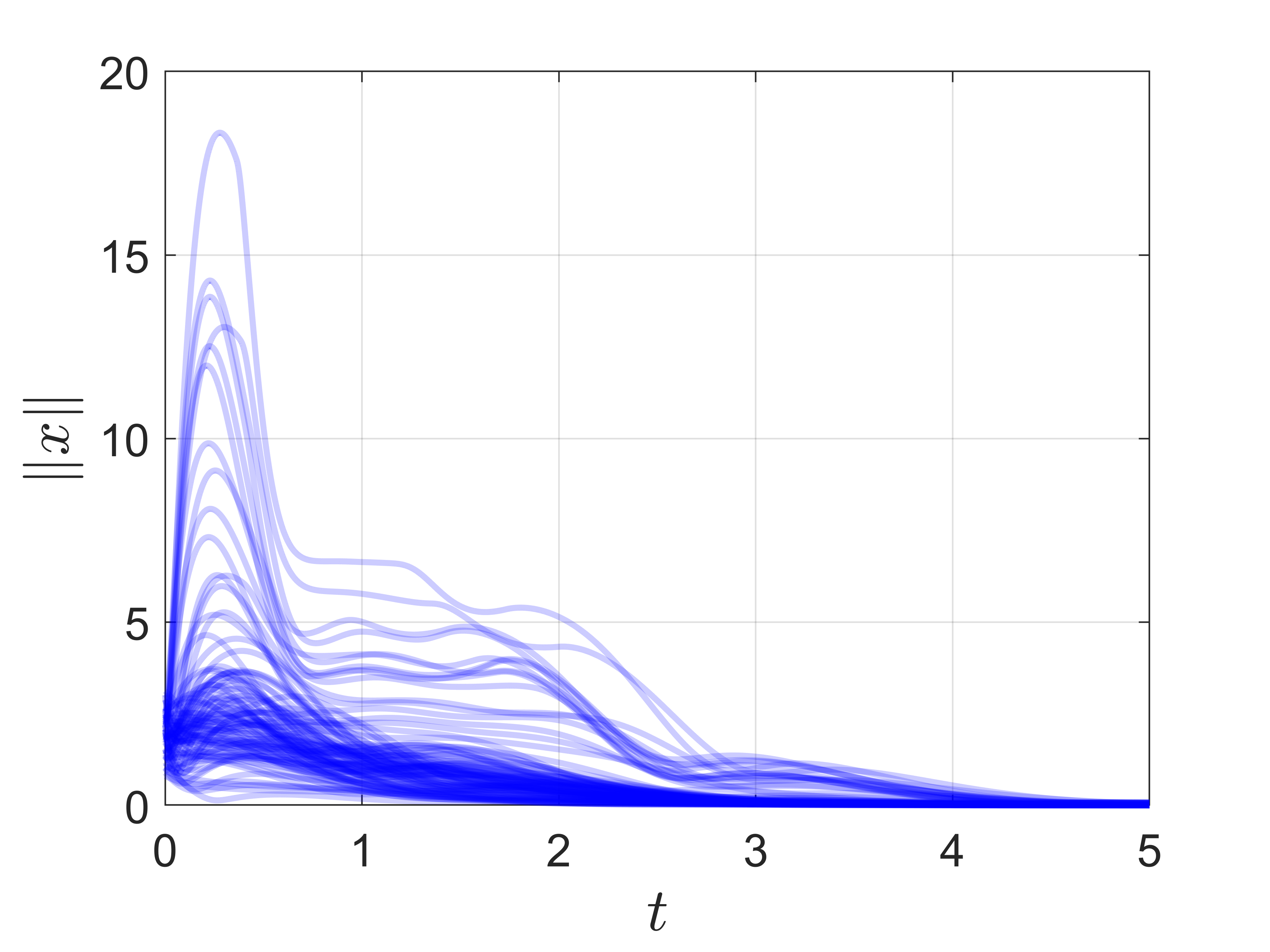
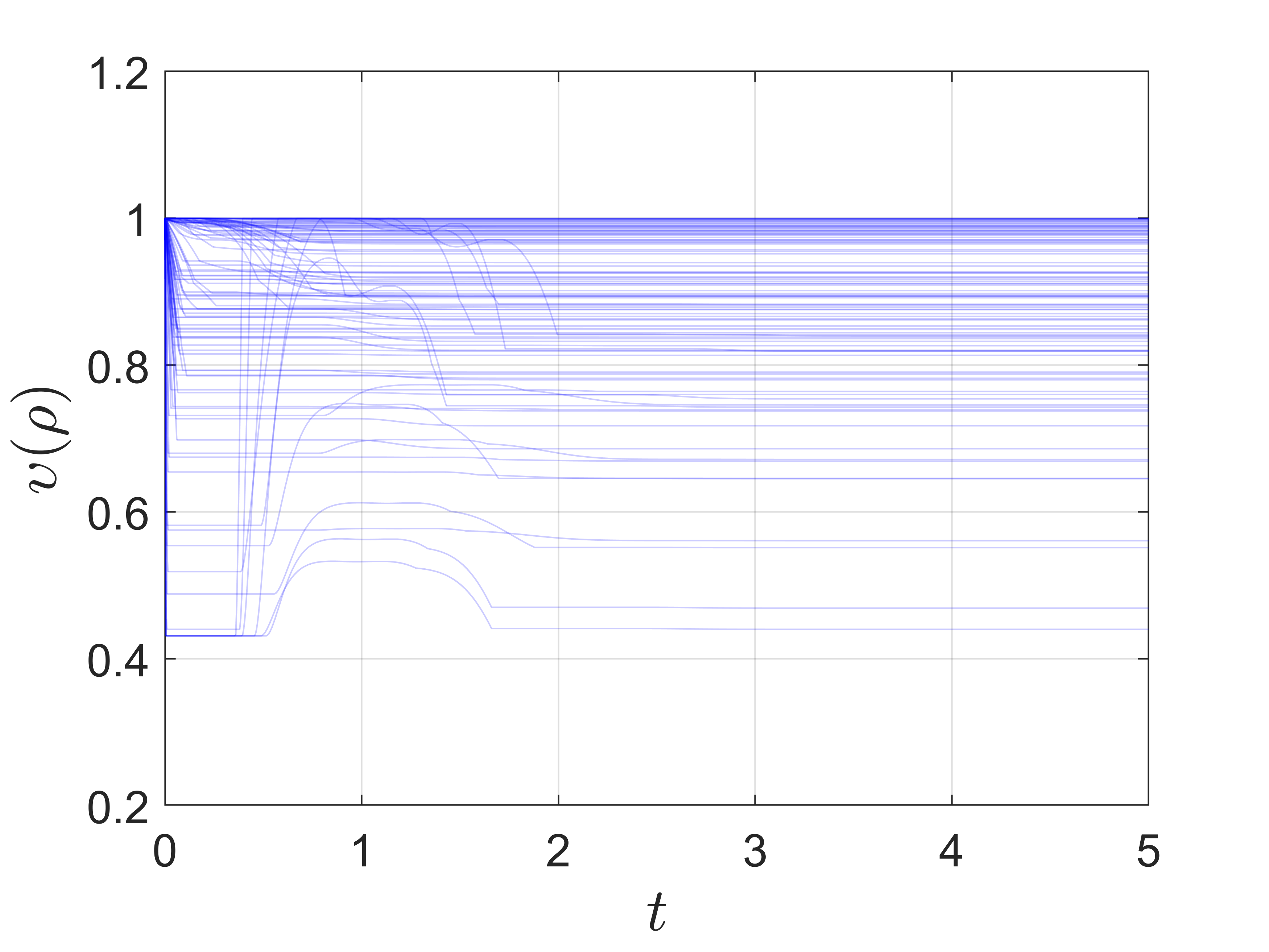
One hundred simulation experiments were conducted with different initial conditions $x_{0}$ and model parameters $\theta^{*}$ to evaluate the performance of the proposed adaptive controller. Fig. 1(a) shows the norm of the state vector $x$ converges to the origin for each trial as desired; 11% of the trials without adaptation failed resulting in the closed-loop system diverging. The scaling function $\upsilon(\rho)$ for each trial is seen in Fig. 1(b) and shows the adaptation rate adjusting in the majority of trials to maintain stability.

IV-B Example 2: Contracting System

Consider the following system with state $x=[x_{1}~{}x_{2}~{}x_{3}]^{\top}$, unknown parameters $\theta=[\theta_{1}~{}\theta_{2}~{}\theta_{3}~{}\theta_{4}]^{\top}$, and dynamics

$$\left[\begin{array}[]{c}\dot{x}_{1}\\ \dot{x}_{2}\\ \dot{x}_{3}\end{array}\right]=\left[\begin{array}[]{c}x_{3}-\theta_{1}x_{1}\\ -x_{2}-\theta_{2}x^{2}_{1}\\ \mathrm{tanh}(x_{2})-\theta_{3}x_{3}-\theta_{4}x_{1}^{2}\end{array}\right]+\left[\begin{array}[]{c}0\\ 0\\ 1\end{array}\right]u.$$ (5)

The system is not feedback linearizable (controllability matrix drops rank at the origin) and is not in strict feedback form. Note that $\theta_{1}$ and $\theta_{2}$ are unmatched parameters. The goal is to track a desired trajectory ($x_{d},~{}u_{d}$) generated with parameters $\theta_{d}=[\hat{\theta}_{1}\,\hat{\theta}_{2}\,0\,0]^{\top}$ driven by a reference $x_{1d}(t)=\mathrm{sin}(t)$. The true model parameters were $\theta^{*}=[-0.3\,-0.8\,-0.25\,-0.75]^{\top}$. The set of allowable parameter variations was ${\theta}\in[-0.4,~{}0.5]\times[-1,~{}0.6]\times[-0.6,~{}0.75]\times[-1.75,~{}0.4]$; each parameter was bounded by the projection operator from [21]. The scaling function was chosen to be $\upsilon(2\rho)=0.9\,e^{\nicefrac{{\rho}}{{5}}}+0.1$ while $\Gamma=5I_{4}$, $\eta=0.1$, and simulation time step $dt=0.01$. A dual uccm was computed using YALMIP and SOS [29]; it was non-flat meaning a quadratic clf does not exist. Geodesics and the pointwise min-norm controller [30] were computed at each time step.

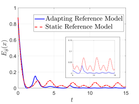
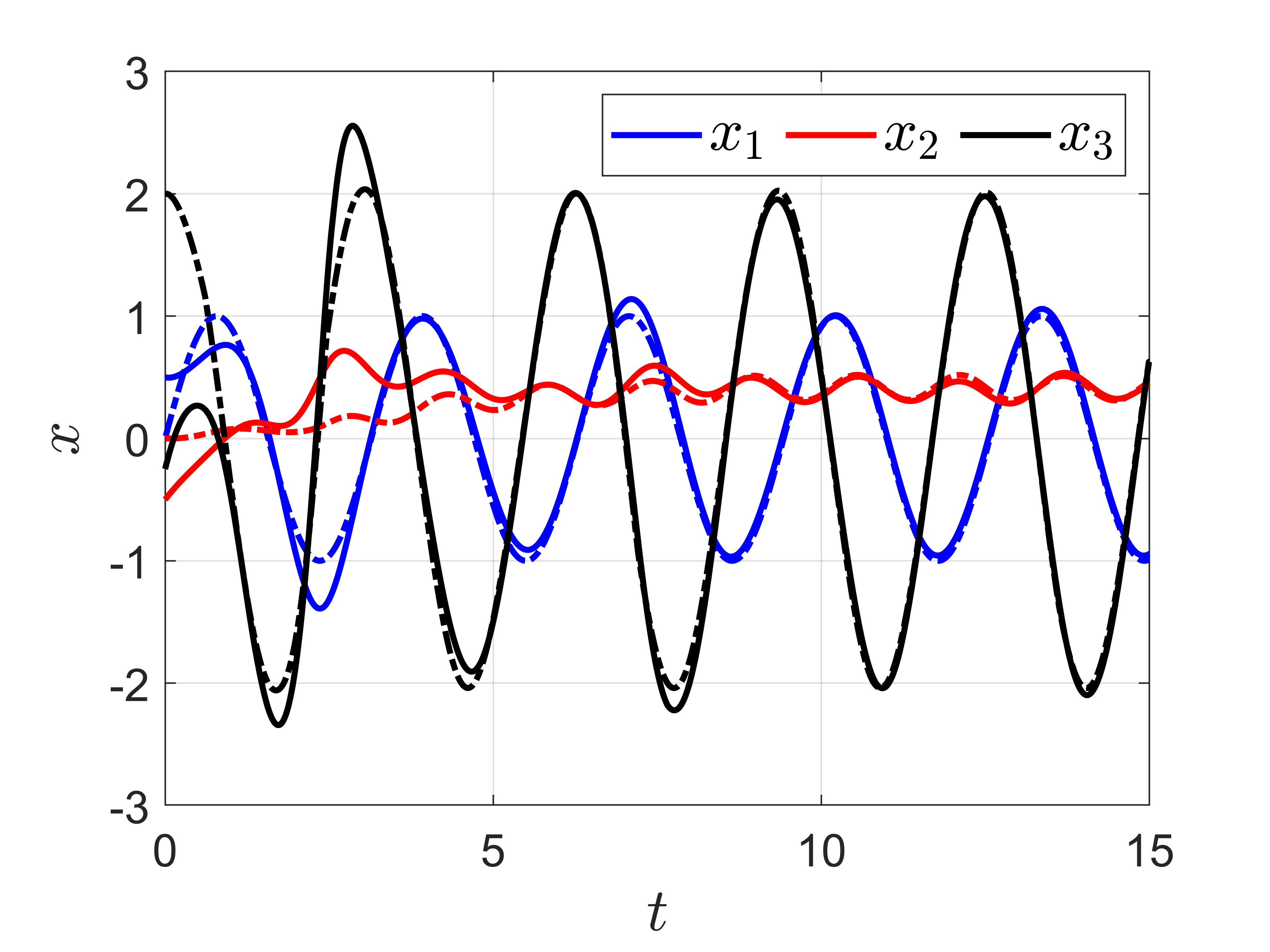
Fig. 2 compares the performance of the proposed controller to a controller that utilizes the same contraction metric but does not adapt to the unmatched parameters, i.e., the reference mode is fixed. The Riemannian energy – an indicator of the closed-loop tracking error – with and without an adaptive reference model is shown in Fig. 2(a). The tracking performance of the proposed approach is superior to that of the controller with a static reference model demonstrating the importance and effectiveness of adapting the reference model with the current parameter estimates. Moreover, Fig. 2(b) confirms that the system will still exhibit the desired behavior (blue curve) despite the reference model changing.

(a)

(b)

Figure 2: Controller comparison with and without an adapting reference model. (a): Riemannian energy of the proposed approach is lower than that of a controller with a static reference model. (b): Closed-loop system exhibits desired behavior (blue) despite the reference model adapting online.

V Concluding Remarks

This work developed a new direct adaptive control technique that eliminates the effects of parameter estimation transients on stability through online adjustment of the adaptation rate. The key advantage of the method is the ability to leverage the certainty equivalence principle in synthesizing stabilizing controllers via Lyapunov or contraction theory for systems with unmatched uncertainties. Several extensions are of interest, including combining the unmatched adaptation law with data-driven controllers for high-dimensional nonlinear systems, e.g., robotic manipulation or mobility; expanding the notion of adaptive safety [31] via certainty equivalence design of barrier functions; and the output feedback with adaptive nonlinear observers. The proposed framework may also be particularly useful in the field of machine learning for dynamical systems, where standard practice is to learn a single feedback policy for all possible model realizations. With the results presented here, the certainty equivalence principle can now be employed to learn a family of optimal policies that then can be later combined with online adaptation to achieve stability despite the presence of uncertainty. Finally, further investigation into the connection between adaptive stabilizability [12] and stabilizability for each $\theta$ is of interest.

VI Appendix

VI-A Adaptive Control Lyapunov Functions

Definition 3 (cf. [12]).

A smooth, positive-definite function $V_{a}:\mathbb{R}^{n}\times\mathbb{R}^{p}\times\mathbb{R}\rightarrow\mathbb{R}_{+}$ is an adaptive control Lyapunov function (aclf) if it is radially unbounded in $x$ and for each $\theta\in\mathbb{R}^{p}$ satisfies

$$\underset{u\in\mathbb{R}^{m}}{\mathrm{inf}} \left\{\frac{\partial V_{a}}{\partial t}+\frac{\partial V_{a}}{\partial x}\left[f-\Delta^{\top}\left(\theta-\Gamma\frac{\partial V_{a}}{\partial\theta}^{\top}\right)+Bu\right]\right\}\leq 0.$$

VI-B Universal Adaptive Control with uccm

Proposition 2.

The system Equation 1 is contracting for each $\theta\in\mathbb{R}^{p}$ if and only if there exists an uccm.

Proof.

“$\Leftarrow$”: Let $\delta V_{\theta}=\delta_{x}^{\top}M_{\theta}(x,t)\delta_{x}$ with uccm $M_{\theta}(x,t)$. Using Definition 2, one can show the implication $\delta_{x}^{\top}M_{\theta}B=0\Rightarrow\dot{\delta V}_{\theta}\leq-2\lambda\delta V_{\theta}$ is true for each $\theta\in\mathbb{R}^{p}$ with uccm $M_{\theta}(x,t)$. Therefore, Equation 1 is contracting for each $\theta\in\mathbb{R}^{p}$.
“$\Rightarrow$”: If Equation 1 is contracting for each $\theta\in\mathbb{R}^{p}$, then there exists a ccm $M_{\theta}(x,t)$ such that the implication $\delta_{x}^{\top}M_{\theta}B=0\Rightarrow\dot{\delta V}_{\theta}\leq-2\lambda\delta V_{\theta}$ is true for $\delta V_{\theta}=\delta_{x}^{\top}M_{\theta}(x,t)\delta_{x}$ and each $\theta\in\mathbb{R}^{p}$. Using the constructive conditions from [18], one arrives to those in Definition 2. Hence, $M_{\theta}(x,t)$ is an uccm.

∎

Proof of Lemma 1.

Since an uccm exists then $\,\frac{d}{dt}\left(\delta_{x}^{\top}M_{\theta}(x,t)\delta_{x}\right)\leq-2\lambda\delta_{x}^{\top}M_{\theta}(x,t)\delta_{x}$. Integrating along a geodesic $\,\gamma(s,t)\,$ yields $\,\dot{E}_{\theta}(x,t)\leq-2\lambda E_{\theta}(x,t)$. ∎

Proof of Theorem 2.

Proof largely follows that of Theorem 1 where $V_{\hat{\theta}}(x,t)=\int_{0}^{1}\gamma_{s}(s,t)^{\top}M_{\hat{\theta}}(\gamma,t)\gamma_{s}(s,t)ds$ and $Q_{\hat{\theta}}(x,t)=2\lambda E_{\hat{\theta}}(x,t)$. Using Lemma 1 and Eqs. 3a and 3b, it can be shown that $\dot{V}_{c}(t)\leq-\lambda\upsilon(\rho)E_{\hat{\theta}}(x,t)$ which implies that both $\,\upsilon(\rho)(E_{\hat{\theta}}(x,t)+\eta)\,$ and $\,\tilde{\theta}\,$ are bounded. Using identical arguments to those in Theorem 1, since $\eta$, $\upsilon(\rho)$, and $\,\upsilon(\rho)(E_{\hat{\theta}}(x,t)+\eta)\,$ are bounded then $E_{\hat{\theta}}(x,t)$ is bounded. Differentiating the right side of $\dot{V}_{c}(t)$,

$$\frac{d}{dt}(\upsilon(\rho)E_{\hat{\theta}}( x,t))=~{}2\upsilon(\rho)\gamma_{s}(s,t)M_{\hat{\theta}}(\gamma(s,t),t)\dot{\gamma}(s,t)\Big{\rvert}^{s=1}_{s=0}$$

$$~{}+\upsilon(\rho)\sum_{i=1}^{p}\left[1-\frac{E_{\hat{\theta}}(x,t)}{E_{\hat{\theta}}(x,t)+\eta}\right]\frac{\partial E}{\partial\hat{\theta}_{i}}\dot{\hat{\theta}}_{i}+\frac{\partial E_{\hat{\theta}}}{\partial t}$$

which is bounded. First note that $E_{\hat{\theta}}(x,t),~{}\tilde{\theta},$ and $\upsilon(\rho)$ are all bounded. Since $E_{\hat{\theta}}(x,t)$ is bounded then $x$ is also bounded for bounded $x_{d}$. Additionally, $\gamma_{s}(s,t)$ is bounded because geodesics have constant speed so $E_{\hat{\theta}}(x,t)=\langle\gamma_{s},\gamma_{s}\rangle_{M_{\hat{\theta}}}$ and since $E_{\hat{\theta}}(x,t)$ is bounded and $M_{\hat{\theta}}(x,t)\succ 0$ then $\gamma_{s}(s,t)$ must also be bounded for all $s\in[0~{}1]$ and $t$. All terms in Equation 3a are bounded so $\smash{\dot{\hat{\small{\theta}}}}$ is also bounded. By smoothness ${\partial E_{\hat{\theta}}/\partial\hat{\theta}_{i}}$ is bounded. Hence $\,\upsilon(\rho)E_{\hat{\theta}}(x,t)\,$ is uniformly continuous. Integrating $\dot{V}_{c}(t)$ yields $\int\limits_{0}^{\infty}\upsilon(\rho(\tau))E_{\hat{\theta}}(x(\tau),\tau)d\tau\leq V_{c}(0)\leq\infty$ so $\,\upsilon(2\rho)E_{\hat{\theta}}(x,t)\rightarrow 0$ by Barbalat’s lemma [21]. Since $\,\upsilon(\rho)>0\,$ uniformly and $\,E_{\hat{\theta}}(x,t)=0\iff x=x_{d}\,$ then $\,x\rightarrow x_{d}\,$ as $t\rightarrow+\infty$. ∎

VI-C Example 1: Backstepping Controller Derivation

The state transformation $z_{\theta}(x)$ for Equation 4 was computed using the standard backstepping technique, which yields

$$z_{\theta,1}(x) =x_{1}$$

$$z_{\theta,2}(x) =x_{2}+2x_{1}-\theta_{2}x_{1}^{2}-\theta_{1}\mathrm{sin}(x_{1})$$

$$z_{\theta,3}(x) =x_{1}+x_{3}+2(-\theta_{2}x_{2}^{2}+x_{2}+x_{1}-\theta_{1}\mathrm{sin}(x_{1}))$$

$$+(\theta_{2}x_{1}^{2}-x_{2}+\theta_{1}\mathrm{sin}(x_{1}))(2\theta_{2}x_{1}-2+\theta_{1}\mathrm{cos}(x_{1})).$$

With the controller Equation 6, the uclf $V_{\theta}(x)=\tfrac{1}{2}z_{\theta}(x)^{\top}z_{\theta}(x)$ satisfies $\dot{V}_{\theta}(x)\leq-4V_{\theta}(x)$ for each $\theta\in\mathbb{R}^{2}$.

 

$$u_{\theta}(x)= \,\,(\theta_{2}x_{1}^{2}-x_{2}+\theta_{1}\mathrm{sin}(x_{1}))\left[(2\theta_{2}x_{1}+\theta_{1}\mathrm{cos}(x_{1}))(2\theta_{2}x_{1}-2+\theta_{1}\mathrm{cos}(x_{1}))+(2\theta_{2}-\theta_{1}\mathrm{sin}(x_{1}))\right.$$

$$\left.(\theta_{2}x_{1}^{2}-x_{2}+\theta_{1}\mathrm{sin}(x_{1}))-2(2\theta_{2}x1-2+\theta_{1}\mathrm{cos}(x_{1}))-1)\right]-2\left[x_{1}+x_{3}+2(-\theta_{2}x_{2}^{2}+x_{2}+2x_{1}-\theta_{1}\mathrm{sin}(x_{1}))\right.$$

$$+\left.(\theta_{2}x_{1}^{2}-x_{2}+\theta_{1}\mathrm{sin}(x_{1}))(2\theta_{2}x_{1}-2+\theta_{1}\mathrm{cos}(x_{1}))\right]-x_{2}-2x_{1}+\theta_{2}x_{1}^{2}+\theta_{1}\mathrm{sin}(x_{1})$$

$$+x_{3}(2\theta_{2}x_{1}-4+\theta_{1}\mathrm{cos}(x_{1}))$$ (6)

 

Acknowledgements: The authors thank Sumeet Singh for his specific suggestions on an early draft of the manuscript.

References

- [1] J.-J. E. Slotine and J. Coetsee, “Adaptive sliding controller synthesis for non-linear systems,” International Journal of Control, vol. 43, no. 6, pp. 1631–1651, 1986.
- [2] J.-J. E. Slotine and W. Li, “On the adaptive control of robot manipulators,” International Journal of Robotics Research, vol. 6, no. 3, 1987.
- [3] D. Taylor, P. Kokotovic, R. Marino, and I. Kanellakopoulos, “Adaptive regulation of nonlinear systems with unmodeled dynamics,” IEEE Transactions on automatic control, vol. 34, no. 4, pp. 405–412, 1989.
- [4] S. Sastry and A. Isidori, “Adaptive control of linearizable systems,” IEEE Transactions on automatic control, vol. 34, no. 11, 1989.
- [5] I. Kanellakopoulos, P. V. Kokotovic, and R. Marino, “An extended direct scheme for robust adaptive nonlinear control,” Automatica, vol. 27, no. 2, pp. 247–255, 1991.
- [6] J. Tsinias, “A theorem on global stabilization of nonlinear systems by linear feedback,” Systems & control letters, vol. 17, no. 5, 1989.
- [7] I. Kanellakopoulos, P. Kokotovic, and A. Morse, “Systematic design of adaptive controllers for feedback linearizable systems,” IEEE Transactions on Automatic Control, vol. 36, no. 11, pp. 1241–1253, 1991.
- [8] M. Krstić, I. Kanellakopoulos, and P. Kokotović, “Adaptive nonlinear control without overparametrization,” Systems & Control Letters, vol. 19, no. 3, pp. 177–185, 1992.
- [9] J. Tsinias, “Backstepping design for time-varying nonlinear systems with unknown parameters,” Systems & Control Letters, vol. 39, no. 4, pp. 219–227, 2000.
- [10] M. Krstic, P. V. Kokotovic, and I. Kanellakopoulos, Nonlinear and adaptive control design. John Wiley & Sons, 1995.
- [11] N. M. Boffi and J.-J. E. Slotine, “Implicit regularization and momentum algorithms in nonlinearly parameterized adaptive control and prediction,” Neural Computation, vol. 33, no. 3, pp. 590–673, 2021.
- [12] M. Krstić and P. V. Kokotović, “Control lyapunov functions for adaptive nonlinear stabilization,” Systems & Control Letters, vol. 26, no. 1, pp. 17–23, 1995.
- [13] N. M. Boffi, S. Tu, and J.-J. E. Slotine, “Regret bounds for adaptive nonlinear control,” in Learning for Dynamics and Control, pp. 471–483, PMLR, 2021.
- [14] R. M. Sanner and J.-J. E. Slotine, “Gaussian networks for direct adaptive control,” in 1991 American control conference, pp. 2153–2159, IEEE, 1991.
- [15] N. M. Boffi, S. Tu, and J.-J. E. Slotine, “Random features for adaptive nonlinear control and prediction,” arXiv:2106.03589, 2021.
- [16] B. T. Lopez and J.-J. E. Slotine, “Adaptive nonlinear control with contraction metrics,” IEEE Control Systems Letters, vol. 5, no. 1, pp. 205–210, 2020.
- [17] W. Lohmiller and J.-J. E. Slotine, “On contraction analysis for non-linear systems,” Automatica, vol. 34, no. 6, pp. 683–696, 1998.
- [18] I. R. Manchester and J.-J. E. Slotine, “Control contraction metrics: Convex and intrinsic criteria for nonlinear feedback design,” IEEE Transactions on Automatic Control, vol. 62, no. 6, pp. 3046–3053, 2017.
- [19] Z. Artstein, “Stabilization with relaxed controls,” Nonlinear Analysis: Theory, Methods & Applications, vol. 7, no. 11, pp. 1163–1173, 1983.
- [20] E. D. Sontag, “A ‘universal’construction of artstein’s theorem on nonlinear stabilization,” Systems & control letters, vol. 13, no. 2, pp. 117–123, 1989.
- [21] J.-J. E. Slotine and W. Li, Applied nonlinear control. Prentice Hall, 1991.
- [22] W. Wang and J.-J. E. Slotine, “On partial contraction analysis for coupled nonlinear oscillators,” Biological cybernetics, vol. 92, no. 1, pp. 38–53, 2005.
- [23] J.-J. E. Slotine, “Modular stability tools for distributed computation and control,” International Journal of Adaptive Control and Signal Processing, vol. 17, no. 6, pp. 397–416, 2003.
- [24] P. A. Ioannou and J. Sun, Robust adaptive control. Courier Corporation, 2012.
- [25] P. Giesl, B. Hamzi, M. Rasmussen, and K. Webster, “Approximation of lyapunov functions from noisy data.,” Journal of Computational Dynamics, vol. 7, no. 1, 2020.
- [26] N. M. Boffi, S. Tu, N. Matni, J.-J. E. Slotine, and V. Sindhwani, “Learning stability certificates from data,” CoRL, 2020.
- [27] H. Tsukamoto, S.-J. Chung, and J.-J. Slotine, “Learning-based adaptive control via contraction theory,” arXiv:2103.02987, 2021.
- [28] S. Richards, N. Azizan, J.-J. Slotine, and M. Pavone, “Adaptive-control-oriented meta-learning for nonlinear systems,” in Robotics science and systems, 2021.
- [29] J. Löfberg, “Yalmip : A toolbox for modeling and optimization in matlab,” in In Proceedings of the CACSD Conference, (Taipei, Taiwan), 2004.
- [30] J. A. Primbs, V. Nevistic, and J. C. Doyle, “A receding horizon generalization of pointwise min-norm controllers,” IEEE Transactions on Automatic Control, vol. 45, no. 5, pp. 898–909, 2000.
- [31] B. T. Lopez, J.-J. E. Slotine, and J. P. How, “Robust adaptive control barrier functions: An adaptive and data-driven approach to safety,” IEEE Control Systems Letters, vol. 5, no. 3, pp. 1031–1036, 2020.