A hybrid Fourier–Real Gaussian Mixture method for fast galaxy–PSF convolution
Abstract
I present a method for the fast convolution of a model galaxy profile by a point-spread function (PSF) model represented as a pixel grid. The method relies upon three observations: First, most simple radial galaxy profiles of common interest (deVaucouleurs, exponential, Sérsic) can be approximated as mixtures of Gaussians. Second, the Fourier transform of a Gaussian is a Gaussian, thus the Fourier transform of a mixture-of-Gausssian approximation of a galaxy can be directly evaluated as a mixture of Gaussians in Fourier space. Third, if a mixture component would result in Fourier-space aliasing, that component can be evaluated in real space. For mixture components to be evaluated in Fourier space, we use the FFT for the PSF model, direct evaluation of the Fourier transform for the galaxy, and the inverse-FFT to return the result to pixel space. For mixture components to be evaluated in real space—which only happens when the mixture components is much larger than the PSF—we use a simple Gaussian approximation of the PSF, perform the convolution analytically, and evaluate in real pixel space. The method is fast and exact (to the extent that the mixture-of-Gaussians approximation of the galaxy profile is exact) as long as the pixelized PSF model is well sampled. This Fourier method can be seen as a way of applying a perfect low-pass filter to the (typically strongly undersampled) galaxy profile before convolution by the PSF, at exactly the Nyquist frequency of the PSF pixel model grid. In this way, it avoids the computational expense of a traditional super-resolution approach. This method allows the efficient use of pixelized PSF models (ie, a PSF represented as a grid of pixel values) in galaxy forward model-fitting approaches such as the Tractor.
1 Introduction
A number of codes exist to render images of galaxies as they would appear when observed with a (real or imagined) telescope and camera, and given observing conditions (sky brightness, atmosphere). These include GalSim (Rowe et al., 2015), Ufig (Bergé et al., 2013), phosim (Peterson et al., 2015), galfit (Peng et al., 2002), ngmix (Sheldon, 2014), the Tractor (Lang et al., in prep), and several others.
In codes that simulate at the pixel level rather than the photon level, it is necessary to convolve a galaxy’s appearance “above the atmosphere” (at high resolution and before any effects from the atmosphere, optics, or detector) by the point-spread function to produce the image as it would appear on the CCD. This step often dominates the computation time required to render a galaxy. Since model galaxy profiles such as the deVaucouleurs profile are very “peaky”, typical galaxy images “above the atmosphere” are undersampled by the native resolution of the CCD. Thus it is not possible to render naïvely the above-the-atmosphere galaxy at native pixel scale and then convolve by the PSF (also represented at native pixel scale), because undersampling will lead to aliasing. Codes typically attempt to render the images at higher resolution than the CCD pixels and then bin down to the native CCD resolution; this significantly increases the computational cost, and may still not achieve exactly correct results.
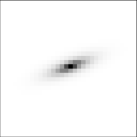
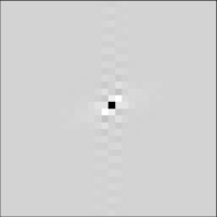
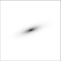
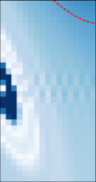
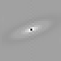
As an illustration of this problem, consider the limit of a tiny, point-like galaxy. If rendered “above the atmosphere” at the native image pixel scale, nearly all its light will appear in one pixel, regardless of its position within that pixel. If we generate a series of images, scanning the galaxy across different subpixel positions in the image, the galaxy’s pixelized light will jump from one pixel to the next in steps. When convolved by the PSF, the galaxy will look like a point source in the image, but rather than moving smoothly will jump from one pixel to the next. If rendered at twice the native pixel scale and binned, it will jump in half-pixel steps, and if rendered at four times the native pixel resolution, will jump in quarter-pixel steps. This occurs because the “above the atmosphere” image is undersampled; a point source has power at all frequencies, and rendering it at the native pixel scale causes the high-frequency power to alias into the band, causing errors in the rendering. As example of this is shown in Figure 3.
Some of the codes mentioned above, and in particular GalSim, provide the option to render PSF-convolved galaxies in Fourier space. To avoid the aliasing discussed above, it is necessary to evaluate the Fourier transform of the galaxy profile directly in Fourier space. For exponential galaxy profiles, the GalSim authors give an analytic expression. For deVaucouleurs and Sérsic profiles, however, a look-up table must be used, and they caution that a separate look-up table must be pre-computed for each Sérsic index, which can dominate the computational cost. Finally, due to the periodic nature of the inverse Fourier transform, spatial aliasing can occur if the galaxy profile is rendered into an image that is too small (as illustrated in Figure 2). If the GalSim user requests such a rendering, it produces the rendering on a larger image (possibly at considerable extra cost) and returns the un-aliased sub-image. The hybrid Fourier/real method presented here provides an inexpensive alternative.
In the Tractor, we have previously taken the approach of using mixture-of-Gaussian approximations111 A mixture of Gaussians is a weighted sum of Gaussian components, with . for both the PSF and the model galaxy profiles. The galaxy profile approximations are presented in Hogg & Lang (2013), and we use direct chi-squared minimization to fit mixture-of-Gaussian models to pixelized PSF models. With the PSF and galaxy represented as mixtures of Gaussians, convolution is analytic and results in a larger mixture of Gaussians (the product of the two mixture sizes), which can then be directly evaluated in pixel space. This approach has the distinct limitation that the PSF must be approximated as a mixture of Gaussians; in practice, it takes many Gaussians to achieve a good approximation, and this makes the computation expensive.
In this work, I consider pixelized PSF models, such as those produced by PsfEx (Bertin, 2011). Since these models are created from real images, they are naturally pixel-convolved models; that is, they already include the effect of being sampled by square pixels.
The galaxy models considered here are simple elliptical isophotes with surface brightness defined, as a functional of radius , by
| (1) |
where we can fix (exponential profile), (deVaucouleurs profile), or fit for (Sérsic profile). It is also common to fit for a linear combination of and profiles (“bulge-disk decomposition” or “composite galaxy profile”). The term is a scalar, usually defined for each so that half the light falls within . The elliptical shape can be represented in terms of effective radius, axis ratio, and position angle, or a variety of other ellipse representations.
| Step 1: PSF | FFT(PSF) | |
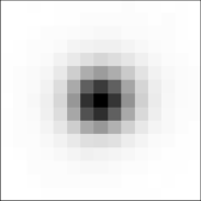 |
 |
|
| Step 3: Galaxy MoG | Step 5: FT(MoG) | Step 6: FT(Galaxy) |
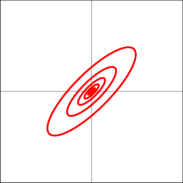 |

|
 |
| PSF Galaxy | FT(PSF Galaxy) | |
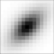 |
 |
2 The method
The method presented here builds directly upon our mixture-of-Gaussians approximation of galaxy profiles, with the realization that the Fourier transform of a Gaussian is also a Gaussian. This allows us to evaluate the Fourier transform of a model galaxy profile directly in Fourier space, without ever having to render the “above the atmosphere” (unconvolved) galaxy profile in pixel space. We can then multiply this Fourier-space representation of the galaxy by the Fourier transform of the pixelized PSF model, then inverse Fourier transform back to pixel space to get the PSF-convolved galaxy profile. As long as the pixelized PSF model is well sampled, this method produces exact answers for each Gaussian in the mixture.
We will elaborate on each step of the method below. In summary:
-
1.
Choose the desired output image size and embed the pixelized PSF model in a zero-padded image of this size.
-
2.
Compute the Fourier Transform of the padded PSF model via the Fast Fourier Transform (FFT), recording the frequencies of the FFT terms.
-
3.
Transform the mixture-of-Gaussians approximation of the model galaxy through an ellipticity matrix and the local image World Coordinate System (WCS) matrix to get pixel-space Gaussians (optionally including sub-pixel shifts).
-
4.
Determine which (if any) components of the mixture-of-Gaussians galaxy model are large enough to produce significant spatial aliasing in the chosen output image size; omit these from the Fourier-space evaluation and evaluate in real space instead.
-
5.
Convert the galaxy mixture-of-Gaussians from pixel space to Fourier space, analytically.
-
6.
Evaluate the Fourier-space Gaussians on the frequency grid .
-
7.
Multiply the PSF and galaxy Fourier transforms, then inverse-FFT back to pixel space.
-
8.
Add any galaxy Gaussian mixture terms evaluated in real space, then, optionally, use Lanczos interpolation to perform sub-pixel shifting, if not done in Fourier space.
The process is illustrated in Figure 1. Example code is available alongside the paper source,222 Available at https://github.com/dstndstn/fft-gal-convolution. and the method is also implemented in the Tractor code.333Available at https://github.com/dstndstn/tractor.
Step 1, choosing the desired output image size, depends on the size of the PSF model as well as the galaxy. If the chosen size is too small, wrap-around spatial aliasing will occur since the FFT is periodic. This is mitigated by Step 4 (evaluating galaxy mixture-of-Gaussian terms that will result in aliasing in real space rather than Fourier space), but it remains necessary to choose a large enough output image to capture a sufficient fraction of the light from the galaxy model. In practice, one would likely choose the PSF size plus some factor of the galaxy half-light radius to capture a sufficient fraction of the flux, or, taking the brightness of the galaxy into account, a sufficient surface brightness accuracy.
In Step 2, we compute the FFT of the PSF. If the PSF is constant across the image, this FFT need only be computed once per image. Alternatively, some PSF modelling tools, including PsfEx (Bertin, 2011), produce eigen-PSF models. That is, the PSF model varies spatially across the image, and the variation is represented as polynomial variations in the amplitudes of a set of pixelized PSF components. This is convenient, since the FFT of each eigen-component can be computed once in preprocessing and the FFT at a given position in the image can be computed by weighting the component FFTs using the PSF model’s polynomial spatial variation terms.
In Step 3, we transform the mixture-of-Gaussians approximation of the galaxy profiles from their representation in units of galaxy effective radius into pixel units. This includes an ellipse transformation (scaling by effective radius, shearing by galaxy axis ratio, rotation by galaxy position angle), plus a transformation into pixel coordinates based on a locally-linear approximation of the image’s World Coordinate System. The result is a pixel-space mixture-of-Gaussians representation of the galaxy.
Specifically, in the Tractor, we prefer to represent the shape of a galaxy by the effective radius and two ellipticity components and as are typically used in weak lensing. We can represent this as a matrix that transforms from celestial coordinates into units of effective radius (the coordinates in which the galaxy profiles are written). This is most easily done by computing the position angle and axis ratio ,
| (2) | ||||
| (3) | ||||
| (4) |
leading to the transformation matrix
| (5) |
If we represent the local astrometric world coordinate system by an affine transformation that takes celestial coordinates to pixel coordinates, then we can multiply the two transformation matrices to convert from pixels to galaxy profile coordinates. The FITS WCS standard (Calabretta & Greisen, 2002) defines a transformation matrix that takes pixels to intermediate world coordinates. The combined affine transformation matrix is then
| (6) |
so that a covariance matrix in galaxy effective radius coordinates can be transformed into pixel space by computing
| (7) |
where the galaxy profile’s variances are isotropic; . When we write out this matrix in full, we find that the and terms always appear in pairs, so we can avoid computing these trigonometric functions explicitly in the above. See Appendix A.
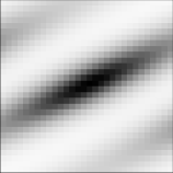
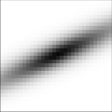
In Step 4, we determine which components of the mixture-of-Gaussians representation of the galaxy profile will result in significant spatial aliasing in the FFT. In the Tractor, we compute the sum of the diagonal elements of the pixel-space covariance matrix , take the square root and divide this by half the output image size; this is roughly the number of ‘sigmas’ from the center to the edge of the image, for that Gaussian component. For Gaussian mixture components where this is greater than , we evaluate in Fourier space. For components less than , we evaluate in real space. For components between and , we compute both real and Fourier versions and ramp smoothly between them, so that the galaxy profile has continuous first derivatives. To evaluate in real space, we use a single-Gaussian approximation of the PSF. Since this approximate PSF model is only used when the galaxy model is much larger than the PSF, this approximation is reasonable. See Figure 2.
| -pixel FFT | FFT | Hybrid |
|---|---|---|
 |
 |
 |
Step 5 is the core of the method. The Fourier transform of a Gaussian is another Gaussian; our mixture-of-Gaussian representation of galaxy profiles can be converted into a mixture of Gaussians in Fourier space. A single 2-dimensional Gaussian centered at the origin and with covariance in pixel space is defined by
| (8) |
which becomes, writing out the pixel coordinate vector as and symmetric covariance ,
| (9) |
We can perform sub-pixel shifts of the galaxy model either in Fourier space, or by Lanczos convolution in pixel space. If we choose to shift in Fourier space, the Fourier Transform of the shifted Gaussian is defined as
| (10) |
and we use the shift theorem to move the centroid to in pixel space via a phase term in Fourier space;
| (11) |
which, plugging in the covariance matrix , works out to
| (12) |
which can easily be evaluated on a grid of frequencies . This is the expression we must evaluate to produce the Fourier transform of a single Gaussian component of a galaxy model. Recall that the values , and are simple manipulations of the galaxy radius and ellipticity and the local astrometric transformation, while and handle sub-pixel shifts.
For a mixture of Gaussians, we must evaluate for each component in the mixture and compute their weighted sum. In the case of a mixture-of-Gaussians representation of affine-transformed galaxy profiles, the centers are the same for each component in the mixture; only the covariances, , differ. The Fourier transform of a mixture of Gaussians,
| (13) |
is therefore
| (14) |
In practice, computing the phase shift in Fourier space requires many and operations, so in the Tractor we instead use Lanczos interpolation to perform sub-pixel shifting of the final pixel-space model. This also has the desirable effect that galaxy models with tiny radius approach point-source models, to higher precision than we find in practice when using Fourier phase shifts.
In Step 6 of our method, we directly evaluate these Gaussians in Fourier space, on the same discrete frequency grid used for the FFT of the PSF. This has interesting properties. By taking the Fourier transform, we are effectively assuming that the PSF model is well sampled, thus has zero power outside the frequency grid of the FFT. The galaxy profile may have power outside that frequency range; this is the reason that one cannot simply render the galaxy profile “above the atmosphere” at the native image pixel scale and apply FFT convolution naïvely: In the limit, a point-like galaxy has power at all frequencies. But when we multiply the PSF and galaxy profile in Fourier space, all that high-frequency power will be zeroed out by the assumption of a well-sampled PSF model. Effectively, by evaluating the galaxy Fourier transform directly in the frequency space of the PSF model, we are applying a perfect low-pass filter at exactly the Nyquist limit. By zeroing out the high-frequency power, we avoid the aliasing that would otherwise result from Fourier transforming an undersampled signal.
In Step 7, we multiply the PSF and galaxy Fourier transforms, and apply the inverse FFT to return to pixel space. Finally, in Step 8, we add in the Gaussian mixture terms that were evaluated in real space, and, if not done in Fourier space, use Lanczos interpolation to perform a sub-pixel shift.
3 Discussion
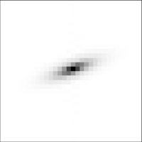
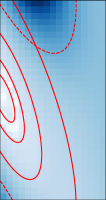
This method for convolution of astronomical galaxy profiles with point spread functions is both accurate and computationally efficient. The accuracy is demonstrated in Figure 3, surpassing the accuracy of the significantly more expensive approach of using sub-pixel bins in real space. This method handles the real-world complications of elliptical galaxy shapes and more complex galaxy profiles such as Sérsic profiles. Code implementing the method is publicly available in the Tractor444https://github.com/dstndstn/tractor.
| This method | log((This)) | |||
 |
 |
|||
| Naïve | log((Naïve)) | (Naïve This) | Naïve This | |
 |
 |
 |
 |
 |
| Double-resolution | log((Double)) | (Double This) | Double This | |
 |
 |
 |
 |
 |
A lot of the computational cost of this method is in evaluating the exp function rather than in the FFT or inverse-FFT, so fast exp approximations555For example, https://github.com/herumi/fmath as used in ngmix, https://github.com/esheldon/ngmix. could provide significant speedups.
The method is implemented in the Tractor code and has been used at scale in the data reduction for the DESI Legacy Imaging Surveys (Dey et al., 2019), which include square degrees of imaging data from three different cameras (the Dark Energy Camera (Flaugher et al., 2015), the 90Prime camera (Williams et al., 2004), and the Mosaic3 camera (Dey et al., 2016)), measuring over two billion sources through forward modeling.
As mentioned earlier, when rendering Sérsic or deVaucoulers galaxy models in Fourier space, GalSim must pre-compute look-up tables for the Fourier transforms, with a different table required for each Sérsic index. The expense of this operation means that the GalSim authors recommend using only discrete Sérsic indices. We have recently found that the Gaussian mixture components (amplitudes and variances) for Sérsic galaxies vary smoothly with respect to Sérsic index, so we can fit for a discrete set of indices and then interpolate for intermediate values. This allows us to evaluate general Sérsic models for the same computational cost as exponential or deVaucoulers models. Indeed, our latest Legacy Surveys release, Data Release 9, performs these fits at scale and reports general Sérsic fits for millions of galaxies.
Appendix A Galaxy variances in pixel space
Writing out the matrix multiplication in Equation 7 assuming an isotropic variance , we get the pixel-space covariance matrix
| (A1) |
where the matrix is symmetric so that and the terms are
| (A2) | ||||
| (A3) | ||||
| (A4) | ||||
| (A5) |
where is the galaxy effective radius in degrees, is the axis ratio (Equation 4) and we have defined the abbreviations
| (A6) | ||||
| (A7) | ||||
| (A8) |
where the matrix terms have units of degrees per pixel. Observe that the covariance terms only contain , , and terms. We can therefore use the identities:
| (A9) | ||||
| (A10) | ||||
| (A11) |
where and are the two ellipticity components and . This allows us to avoid computing , and explicitly when transforming a galaxy into pixel space.
References
- Bergé et al. (2013) Bergé, J. et al., 2013, Astronomy and Computing, 1, 23; arXiv:1209.1200
- Bertin (2011) Bertin, E., 2011, ADASS XX, ASP Conference Series, 442, 435
- Calabretta & Greisen (2002) Calabretta, M. R. & Greisen, E. W., 2002, Astronomy & Astrophysics, 395, 1077; arXiv:astro-ph/0207413
- Dey et al. (2016) Dey, A., Rabinowitz, D. et al., 2016, in Proc. SPIE, 9908, Ground-based and Airborne Instrumentation for Astronomy VI, 99082C
- Dey et al. (2019) Dey, A., Schlegel, D.J., et al., 2019, AJ, 157, 168; arXiv:1804.08657
- Flaugher et al. (2015) Flaugher, B. et al., 2015, AJ, 150, 150; arXiv:1504.02900
- Hogg & Lang (2013) Hogg, D. W. & Lang, D., 2013, PASP, 125, 719; arXiv:1210.6563
- Peng et al. (2002) Peng, C. Y. et al., 2002, AJ, 124, 266; arXiv:0204182
- Peterson et al. (2015) Peterson, J. R. et al., 2015, ApJS, 218, 14; arXiv:1504.06570
- Rowe et al. (2015) Rowe, B. et al., 2015, Astronomy and Computing, 10, 121; arXiv:1407.7676
- Sheldon (2014) Sheldon, E. S., 2014, MNRAS, 444, 25; arXiv:1403.7669
- Williams et al. (2004) Williams, G. G et al., 2014, SPIE Conference Series, 5492, Ground-based Instrumentation for Astronomy, 787W