Scaling Replicated State Machines with Compartmentalization

Abstract.

State machine replication protocols, like MultiPaxos and Raft, are a critical component of many distributed systems and databases. However, these protocols offer relatively low throughput due to several bottlenecked components. Numerous existing protocols fix different bottlenecks in isolation but fall short of a complete solution. When you fix one bottleneck, another arises. In this paper, we introduce compartmentalization, the first comprehensive technique to eliminate state machine replication bottlenecks. Compartmentalization involves decoupling individual bottlenecks into distinct components and scaling these components independently. Compartmentalization has two key strengths. First, compartmentalization leads to strong performance. In this paper, we demonstrate how to compartmentalize MultiPaxos to increase its throughput by $6\times$ on a write-only workload and $16\times$ on a mixed read-write workload. Unlike other approaches, we achieve this performance without the need for specialized hardware. Second, compartmentalization is a technique, not a protocol. Industry practitioners can apply compartmentalization to their protocols incrementally without having to adopt a completely new protocol.

PVLDB Reference Format:
PVLDB, 14(1): XXX-XXX, 2020.
doi:XX.XX/XXX.XX

PVLDB Artifact Availability:
The source code, data, and/or other artifacts have been made available at http://vldb.org/pvldb/format_vol14.html.

1. Introduction

State machine replication protocols are a crucial component of many distributed systems and databases (Corbett et al., 2013; Thomson et al., 2012; Burrows, 2006; Taft et al., 2020; cos, [n.d.]; tid, [n.d.]; yug, [n.d.]; cas, [n.d.]). In many state machine replication protocols, a single node has multiple responsibilities. For example, a Raft leader acts as a batcher, a sequencer, a broadcaster, and a state machine replica. These overloaded nodes are often a throughput bottleneck, which can be disastrous for systems that rely on state machine replication.

Many databases, for example, rely on state machine replication to replicate large data partitions of tens of gigabytes (Schultz et al., 2019; cos, [n.d.]). These databases require high-throughput state machine replication to handle all the requests in a partition. However, in such systems, it is not uncommon to exceed the throughput budget of a partition. For example, Cosmos DB will split a partition if it experiences high throughput despite being under the storage limit. The split, aside from costing resources, may have additional adverse effects on applications, as Cosmos DB provides strongly consistent transactions only within the partition. Eliminating state machine replication bottlenecks can help avoid such unnecessary partition splits and improve performance, consistency, and resource utilization.

Researchers have studied how to eliminate throughput bottlenecks, often by inventing new state machine replication protocols that eliminate a single throughput bottleneck (Moraru et al., 2013; Arun et al., 2017; Mao et al., 2008; Ailijiang et al., 2019; Lamport, 2005, 2006; Charapko et al., 2019; Howard et al., 2017; Zhu et al., 2019; Terrace and Freedman, 2009; Biely et al., 2012). However, eliminating a single bottleneck is not enough to achieve the best possible throughput. When you eliminate one bottleneck, another arises. To achieve the best possible throughput, we have to eliminate all of the bottlenecks.

The key to eliminating these throughput bottlenecks is scaling, but it is widely believed that state machine replication protocols don’t scale (Kapritsos and Junqueira, 2010; Zhang et al., 2018; Mao et al., 2008; Moraru et al., 2013; Arun et al., 2017). In this paper, we show that this is not true. State machine replication protocols can indeed scale. As a concrete illustration, we analyze the throughput bottlenecks of MultiPaxos and systematically eliminate them using a combination of decoupling and scaling, a technique we call compartmentalization. For example, consider the MultiPaxos leader, a notorious throughput bottleneck. The leader has two distinct responsibilities. First, it sequences state machine commands into a log. It puts the first command it receives into the first log entry, the next command into the second log entry, and so on. Second, it broadcasts the commands to the set of MultiPaxos acceptors, receives their responses, and then broadcasts the commands again to a set of state machine replicas. To compartmentalize the MultiPaxos leader, we first decouple these two responsibilities. There’s no fundamental reason that the leader has to sequence commands and broadcast them. Instead, we have the leader sequence commands and introduce a new set of nodes, called proxy leaders, to broadcast the commands. Second, we scale up the number of proxy leaders. We note that broadcasting commands is embarrassingly parallel, so we can increase the number of proxy leaders to avoid them becoming a bottleneck. Note that this scaling wasn’t possible when sequencing and broadcasting were coupled on the leader since sequencing is not scalable. Compartmentalization has three key strengths.

(1) Strong Performance Without Strong Assumptions. We compartmentalize MultiPaxos and increase its throughput by a factor of $6\times$ on a write-only workload using $6.66\times$ the number of machines and $16\times$ on a mixed read-write workload using $4.33\times$ the number of machines. Moreover, we achieve our strong performance without the strong assumptions made by other state machine replication protocols with comparable performance (Terrace and Freedman, 2009; Zhu et al., 2019; Van Renesse and Schneider, 2004; Takruri et al., 2020; Jin et al., 2018). For example, we do not assume a perfect failure detector, we do not assume the availability of specialized hardware, we do not assume uniform data access patterns, we do not assume clock synchrony, and we do not assume key-partitioned state machines.

(2) General and Incrementally Adoptable. Compartmentalization is not a protocol. Rather, it’s a technique that can be systematically applied to existing protocols. Industry practitioners can incrementally apply compartmentalization to their current protocols without having to throw out their battle-tested implementations for something new and untested. We demonstrate the generality of compartmentalization by applying it three other protocols (Mao et al., 2008; Biely et al., 2012; Ding et al., 2020) in addition to MultiPaxos.

(3) Easy to Understand. Researchers have invented new state machine replication protocols to eliminate throughput bottlenecks, but these new protocols are often subtle and complicated. As a result, these sophisticated protocols have been largely ignored in industry due to their high barriers to adoption. Compartmentalization is based on the simple principles of decoupling and scaling and is designed to be easily understood.

In summary, we present the following contributions

• We characterize all of MultiPaxos’ throughput bottlenecks and explain why, historically, it was believed that they could not be scaled.

• We introduce the concept of compartmentalization: a technique to decouple and scale throughput bottlenecks.

• We apply compartmentalization to systematically eliminate MultiPaxos’ throughput bottlenecks. In doing so, we debunk the widely held belief that MultiPaxos and similar state machine replication protocols do not scale.

2. Background

2.1. System Model

Throughout the paper, we assume an asynchronous network model in which messages can be arbitrarily dropped, delayed, and reordered. We assume machines can fail by crashing but do not act maliciously; i.e., we do not consider Byzantine failures. We assume that machines operate at arbitrary speeds, and we do not assume clock synchronization. Every protocol discussed in this paper assumes that at most $f$ machines will fail for some configurable $f$.

2.2. Paxos

Consensus is the act of choosing a single value among a set of proposed values, and Paxos (Lamport, 1998) is the de facto standard consensus protocol. We assume the reader is familiar with Paxos, but we pause to review the parts of the protocol that are most important to understand for the rest of this paper.

A Paxos deployment that tolerates $f$ faults consists of an arbitrary number of clients, at least $f+1$ proposers, and $2f+1$ acceptors, as illustrated in Figure 1. When a client wants to propose a value, it sends the value to a proposer $p$. The proposer then initiates a two-phase protocol. In Phase 1, the proposer contacts the acceptors and learns of any values that may have already been chosen. In Phase 2, the proposer proposes a value to the acceptors, and the acceptors vote on whether or not to choose the value. If a value receives votes from a majority of the acceptors, the value is considered chosen.

More concretely, in Phase 1, $p$ sends Phase1a messages to at least a majority of the $2f+1$ acceptors. When an acceptor receives a Phase1a message, it replies with a Phase1b message. When the leader receives Phase1b messages from a majority of the acceptors, it begins Phase 2. In Phase 2, the proposer sends Phase2a$\langle x\rangle$ messages to the acceptors with some value $x$. Upon receiving a Phase2a$\langle x\rangle$ message, an acceptor can either ignore the message, or vote for the value $x$ and return a Phase2b$\langle x\rangle$ message to the proposer. Upon receiving Phase2b$\langle x\rangle$ messages from a majority of the acceptors, the proposed value $x$ is considered chosen.

(a) Phase 1

(b) Phase 2

Figure 1. An example execution of Paxos ($f=1$).

2.3. MultiPaxos

While consensus is the act of choosing a single value, state machine replication is the act of choosing a sequence (a.k.a. log) of values. A state machine replication protocol manages a number of replicas of a deterministic state machine. Over time, the protocol constructs a growing log of state machine commands, and replicas execute the commands in log order. By beginning in the same initial state, and by executing commands in the same order, all state machine replicas are kept in sync. This is illustrated in Figure 2.

(a) $t=0$

(b) $t=1$

(c) $t=2$

(d) $t=3$

Figure 2. At time $t=0$, no state machine commands are chosen. At time $t=1$ command $x$ is chosen in slot $0$. At times $t=2$ and $t=3$, commands $z$ and $y$ are chosen in slots $2$ and $1$. Executed commands are shaded green. Note that all state machines execute the commands $x$, $y$, $z$ in log order.

MultiPaxos is one of the most widely used state machine replication protocols. Again, we assume the reader is familiar with MultiPaxos, but we review the most salient bits. MultiPaxos uses one instance of Paxos for every log entry, choosing the command in the $i$th log entry using the $i$th instance of Paxos. A MultiPaxos deployment that tolerates $f$ faults consists of an arbitrary number of clients, at least $f+1$ proposers, and $2f+1$ acceptors (like Paxos), as well as at least $f+1$ replicas, as illustrated in Figure 3.

Figure 3. An example execution of MultiPaxos ($f=1$). The leader is adorned with a crown.

Initially, one of the proposers is elected leader and runs Phase 1 of Paxos for every log entry. When a client wants to propose a state machine command $x$, it sends the command to the leader (1). The leader assigns the command a log entry $i$ and then runs Phase 2 of the $i$th Paxos instance to get the value $x$ chosen in entry $i$. That is, the leader sends Phase2a$\langle i,x\rangle$ messages to the acceptors to vote for value $x$ in slot $i$ (2). In the normal case, the acceptors all vote for $x$ in slot $i$ and respond with Phase2b$\langle i,x\rangle$ messages (3). Once the leader learns that a command has been chosen in a given log entry (i.e. once the leader receives Phase2b$\langle i,x\rangle$ messages from a majority of the acceptors), it informs the replicas (4). Replicas insert commands into their logs and execute the logs in prefix order.

Note that the leader assigns log entries to commands in increasing order. The first received command is put in entry $0$, the next command in entry $1$, the next command in entry $2$, and so on. Also note that even though every replica executes every command, for any given state machine command $x$, only one replica needs to send the result of executing $x$ back to the client (5). For example, log entries can be round-robin partitioned across the replicas.

2.4. MultiPaxos Doesn’t Scale?

It is widely believed that MultiPaxos does not scale (Kapritsos and Junqueira, 2010; Zhang et al., 2018; Mao et al., 2008; Moraru et al., 2013; Arun et al., 2017). Throughout the paper, we will explain that this is not true, but it first helps to understand why trying to scale MultiPaxos in the straightforward and obvious way does not work. MultiPaxos consists of proposers, acceptors, and replicas. We discuss each.

First, increasing the number of proposers does not improve performance because every client must send its requests to the leader regardless of the number proposers. The non-leader replicas are idle and do not contribute to the protocol during normal operation.

Second, increasing the number of acceptors hurts performance. To get a value chosen, the leader must contact a majority of the acceptors. When we increase the number of acceptors, we increase the number of acceptors that the leader has to contact. This decreases throughput because the leader—which is the throughput bottleneck—has to send and receive more messages per command. Moreover, every acceptor processes at least half of all commands regardless of the number of acceptors.

Third, increasing the number of replicas hurts performance. The leader broadcasts chosen commands to all of the replicas, so when we increase the number of replicas, we increase the load on the leader and decrease MultiPaxos’ throughput. Moreover, every replica must execute every state machine command, so increasing the number of replicas does not decrease the replicas’ load.

3. Compartmentalizing MultiPaxos

We now compartmentalize MultiPaxos. Throughout the paper, we introduce six compartmentalizations, summarized in Table 1. For every compartmentalization, we identify a throughput bottleneck and then explain how to decouple and scale it.

Table 1. A summary of the compartmentalizations presented in this paper.

Compartmentalization	Bottleneck	Decouple	Scale
1 (Section 3.1)	leader	command sequencing and command broadcasting	the number of proxy leaders
2 (Section 3.2)	acceptors	read quorums and write quorums	the number of write quorums
3 (Section 3.3)	replicas	command sequencing and command broadcasting	the number of replicas
4 (Section 3.4)	leader and replicas	read path and write path	the number of read quorums
5 (Section 4.1)	leader	batch formation and batch sequencing	the number of batchers
6 (Section 4.2)	replicas	batch processing and batch replying	the number of unbatchers

3.1. Compartmentalization 1: Proxy Leaders

Bottleneck

The MultiPaxos leader is a well known throughput bottleneck for the following reason. Refer again to Figure 3. To process a single state machine command from a client, the leader must receive a message from the client, send at least $f+1$ Phase2a messages to the acceptors, receive at least $f+1$ Phase2b messages from the acceptors, and send at least $f+1$ messages to the replicas. In total, the leader sends and receives at least $3f+4$ messages per command. Every acceptor on the other hand processes only $2$ messages, and every replica processes either $1$ or $2$. Because every state machine command goes through the leader, and because the leader has to perform disproportionately more work than every other component, the leader is the throughput bottleneck.

Decouple

To alleviate this bottleneck, we first decouple the leader. To do so, we note that a MultiPaxos leader has two jobs. The first is sequencing. The leader sequences commands by assigning each command a log entry. Log entry $0$, then $1$, then $2$, and so on. The second is broadcasting. The leader sends Phase2a messages, collects Phase2b responses, and broadcasts chosen values to the replicas. Historically, these two responsibilities have both fallen on the leader, but this is not fundamental. We instead decouple the two responsibilities. We introduce a set of at least $f+1$ proxy leaders, as shown in Figure 4. The leader is responsible for sequencing commands, while the proxy leaders are responsible for getting commands chosen and broadcasting the commands to the replicas.

Figure 4. An example execution of Compartmentalized MultiPaxos with three proxy leaders ($f=1$). Throughout the paper, nodes and messages that were not present in previous iterations of the protocol are highlighted in green.

More concretely, when a leader receives a command $x$ from a client (1), it assigns the command $x$ a log entry $i$ and then forms a Phase2a message that includes $x$ and $i$. The leader does not send the Phase2a message to the acceptors. Instead, it sends the Phase2a message to a randomly selected proxy leader (2). Note that every command can be sent to a different proxy leader. The leader balances load evenly across all of the proxy leaders. Upon receiving a Phase2a message, a proxy leader broadcasts it to the acceptors (3), gathers a quorum of $f+1$ Phase2b responses (4), and notifies the replicas of the chosen value (5). All other aspects of the protocol remain unchanged.

Without proxy leaders, the leader processes $3f+4$ messages per command. With proxy leaders, the leader only processes $2$. This makes the leader significantly less of a throughput bottleneck, or potentially eliminates it as the bottleneck entirely.

Scale

The leader now processes fewer messages per command, but every proxy leader has to process $3f+4$ messages. Have we really eliminated the leader as a bottleneck, or have we just moved the bottleneck into the proxy leaders? To answer this, we note that the proxy leaders are embarrassingly parallel. They operate independently from one another. Moreover, the leader distributes load among the proxy leaders equally, so the load on any single proxy leader decreases as we increase the number of proxy leaders. Thus, we can trivially increase the number of proxy leaders until they are no longer a throughput bottleneck.

Discussion

Note that decoupling enables scaling. As discussed in Section 2.4, we cannot naively increase the number of proposers. Without decoupling, the leader is both a sequencer and broadcaster, so we cannot increase the number of leaders to increase the number of broadcasters because doing so would lead to multiple sequencers, which is not permitted. Only by decoupling the two responsibilities can we scale one without scaling the other.

Also note that the protocol remains tolerant to $f$ faults regardless of the number of machines. However, increasing the number of machines does decrease the expected time to $f$ failures (this is true for every protocol that scales up the number of machines, not just our protocol). We believe that increasing throughput at the expense of a shorter time to $f$ failures is well worth it in practice because failed machines can be replaced with new machines using a reconfiguration protocol (Lamport, 2001; Ongaro and Ousterhout, 2014). The time required to perform a reconfiguration is many orders of magnitude smaller than the mean time between failures.

3.2. Compartmentalization 2: Acceptor Grids

Bottleneck

After compartmentalizing the leader, it is possible that the acceptors are the throughput bottleneck. It is widely believed that acceptors do not scale: “using more than $2f+1$ [acceptors] for $f$ failures is possible but illogical because it requires a larger quorum size with no additional benefit” (Zhang et al., 2018). As explained in Section 2.4, there are two reasons why naively increasing the number of acceptors is ill-advised.

First, increasing the number of acceptors increases the number of messages that the leader has to send and receive. This increases the load on the leader, and since the leader is the throughput bottleneck, this decreases throughput. This argument no longer applies. With the introduction of proxy leaders, the leader no longer communicates with the acceptors. Increasing the number of acceptors increases the load on every individual proxy leader, but the increased load will not make the proxy leaders a bottleneck because we can always scale them up.

Second, every command must be processed by a majority of the acceptors. Thus, even with a large number of acceptors, every acceptor must process at least half of all state machine commands. This argument still holds.

Decouple

We compartmentalize the acceptors by using flexible quorums (Howard et al., 2017). MultiPaxos—the vanilla version, not the compartmentalized version—requires $2f+1$ acceptors, and the leader communicates with $f+1$ acceptors in both Phase 1 and Phase 2 (a majority of the acceptors). The sets of $f+1$ acceptors are called quorums, and MultiPaxos’ correctness relies on the fact that any two quorums intersect. While majority quorums are sufficient for correctness, they are not necessary. MultiPaxos is correct as long as every quorum contacted in Phase 1 (called a read quorum) intersects every quorum contacted in Phase 2 (called a write quorum). Read quorums do not have to intersect other read quorums, and write quorums do not have to intersect other write quorums.

By decoupling read quorums from write quorums, we can reduce the load on the acceptors by eschewing majority quorums for a more efficient set of quorums. Specifically, we arrange the acceptors into an $r\times w$ rectangular grid, where $r,w\geq f+1$. Every row forms a read quorum, and every column forms a write quorum ($r$ stands for row and for read). That is, a leader contacts an arbitrary row of acceptors in Phase 1 and an arbitrary column of acceptors for every command in Phase 2. Every row intersects every column, so this is a valid set of quorums.

A $2\times 3$ acceptor grid is illustrated in Figure 5. There are two read quorums (the rows $\{a_{1},a_{2},a_{3}\}$ and $\{a_{4},a_{5},a_{6}\}$) and three write quorums (the columns $\{a_{1},a_{4}\}$, $\{a_{2},a_{5}\}$, $\{a_{3},a_{6}\}$). Because there are three write quorums, every acceptor only processes one third of all the commands. This is not possible with majority quorums because with majority quorums, every acceptor processes at least half of all the commands, regardless of the number of acceptors.

Figure 5. An execution of Compartmentalized MultiPaxos with a $2\times 3$ grid of acceptors ($f=1$). The two read quorums—$\{a_{1},a_{2},a_{3}\}$ and $\{a_{4},a_{5},a_{6}\}$—are shown in solid red rectangles. The three write quorums—$\{a_{1},a_{4}\}$, $\{a_{2},a_{5}\}$, and $\{a_{3},a_{6}\}$—are shown in dashed blue rectangles.

Scale

With majority quorums, every acceptor has to process at least half of all state machines commands. With grid quorums, every acceptor only has to process $\frac{1}{w}$ of the state machine commands. Thus, we can increase $w$ (i.e. increase the number of columns in the grid) to reduce the load on the acceptors and eliminate them as a throughput bottleneck.

Discussion

Note that, like with proxy leaders, decoupling enables scaling. With majority quorums, read and write quorums are coupled, so we cannot increase the number of acceptors without also increasing the size of all quorums. Acceptor grids allow us to decouple the number of acceptors from the size of write quorums, allowing us to scale up the acceptors and decrease their load.

Also note that increasing the number of write quorums increases the size of read quorums which increases the number of acceptors that a leader has to contact in Phase 1. We believe this is a worthy trade-off since Phase 2 is executed in the normal case and Phase 1 is only run in the event of a leader failure.

3.3. Compartmentalization 3: More Replicas

Bottleneck

After compartmentalizing the leader and the acceptors, it is possible that the replicas are the bottleneck. Recall from Section 2.4 that naively scaling the replicas does not work for two reasons. First, every replica must receive and execute every state machine command. This is not actually true, but we leave that for the next compartmentalization. Second, like with the acceptors, increasing the number of replicas increases the load on the leader. Because we have already decoupled sequencing from broadcasting on the leader and introduced proxy leaders, this is no longer true, so we are free to increase the number of replicas. In Figure 6, for example, we show MultiPaxos with three replicas instead of the minimum required two.

Scale

If every replica has to execute every command, does increasing the number of replicas decrease their load? Yes. Recall that while every replica has to execute every state machine, only one of the replicas has to send the result of executing the command back to the client. Thus, with $n$ replicas, every replica only has to send back results for $\frac{1}{n}$ of the commands. If we scale up the number of replicas, we reduce the number of messages that each replica has to send. This reduces the load on the replicas and helps prevent them from becoming a throughput bottleneck. In Figure 6 for example, with three replicas, every replica only has to reply to one third of all commands. With two replicas, every replica has to reply to half of all commands. In the next compartmentalization, we’ll see another major advantage of increasing the number of replicas.

Figure 6. An example execution of Compartmentalized MultiPaxos with three replicas as opposed to the minimum required two ($f=1$).

Discussion

Again decoupling enables scaling. Without decoupling the leader and introducing proxy leaders, increasing the number of replicas hurts rather than helps performance.

3.4. Compartmentalization 4: Leaderless Reads

Bottleneck

We have now compartmentalized the leader, the acceptors, and the replicas. At this point, the bottleneck is in one of two places. Either the leader is still a bottleneck, or the replicas are the bottleneck. Fortunately, we can bypass both bottlenecks with a single compartmentalization.

Decouple

We call commands that modify the state of the state machine writes and commands that don’t modify the state of the state machine reads. The leader must process every write because it has to linearize the writes with respect to one another, and every replica must process every write because otherwise the replicas’ state would diverge (imagine if one replica performs a write but the other replicas don’t). However, because reads do not modify the state of the state machine, the leader does not have to linearize them (reads commute), and only a single replica (as opposed to every replica) needs to execute a read.

We take advantage of this observation by decoupling the read path from the write path. Writes are processed as before, but we bypass the leader and perform a read on a single replica by using the idea from Paxos Quorum Reads (PQR) (Charapko et al., 2019). Specifically, to perform a read, a client sends a PreRead$\langle\rangle$ message to a read quorum of acceptors. Upon receiving a PreRead$\langle\rangle$ message, an acceptor $a_{i}$ returns a PreReadAck$\langle w_{i}\rangle$ message where $w_{i}$ is the index of the largest log entry in which the acceptor has voted (i.e. the largest log entry in which the acceptor has sent a Phase2b message). We call this $w_{i}$ a vote watermark. When the client receives PreReadAck messages from a read quorum of acceptors, it computes $i$ as the maximum of all received vote watermarks. It then sends a Read$\langle x,i\rangle$ request to any one of the replicas where $x$ is an arbitrary read (i.e. a command that does not modify the state of the state machine).

When a replica receives a Read$\langle x,i\rangle$ request from a client, it waits until it has executed the command in log entry $i$. Recall that replicas execute commands in log order, so if the replica has executed the command in log entry $i$, then it has also executed all of the commands in log entries less than $i$. After the replica has executed the command in log entry $i$, it executes $x$ and returns the result to the client. Note that upon receiving a Read$\langle x,i\rangle$ message, a replica may have already executed the log beyond $i$. That is, it may have already executed the commands in log entries $i+1$, $i+2$, and so on. This is okay because as long as the replica has executed the command in log entry $i$, it is safe to execute $x$.

Figure 7. An example execution of Compartmentalized MultiPaxos’ read and write path ($f=1$) with a $2\times 2$ acceptor grid. The write path is shown using solid blue lines. The read path is shown using red dashed lines.

Scale

The decoupled read and write paths are shown in Figure 7. Reads are sent to a row (read quorum) of acceptors, so we can increase the number of rows to decrease the read load on every individual acceptor, eliminating the acceptors as a read bottleneck. Reads are also sent to a single replica, so we can increase the number of replicas to eliminate them as a read bottleneck as well.

Discussion

Note that read-heavy workloads are not a special case. Many workloads are read-heavy (Ghemawat et al., 2003; Nishtala et al., 2013; Atikoglu et al., 2012; Moraru et al., 2013). Chubby (Burrows, 2006) observes that fewer than 1% of operations are writes, and Spanner (Corbett et al., 2013) observes that fewer than 0.3% of operations are writes.

Also note that increasing the number of columns in an acceptor grid reduces the write load on the acceptors, and increasing the number of rows in an acceptor grid reduces the read load on the acceptors. There is no throughput trade-off between the two. The number of rows and columns can be adjusted independently. Increasing read throughput (by increasing the number of rows) does not decrease write throughput, and vice versa. However, increasing the number of rows does increase the size (but not number) of columns, so increasing the number of rows might increase the tail latency of writes, and vice versa.

3.5. Correctness

We now define linearizability and prove that our protocol implements linearizable reads.

Linearizability is a correctness condition for distributed systems (Herlihy and Wing, 1990). Intuitively, a linearizable distributed system is indistinguishable from a system running on a single machine that services all requests serially. This makes a linearizable system easy to reason about. We first explain the intuition behind linearizability and then formalize the intuition.

Consider a distributed system that implements a single register. Clients can send requests to the distributed system to read or write the register. After a client sends a read or write request, it waits to receive a response before sending another request. As a result, a client can have at most one operation pending at any point in time.

(a) An example execution

(b) An incorrect linearization

(c) A linearization

Figure 8.

As a simple example, consider the execution illustrated in Figure 8(a) where the $x$-axis represents the passage of time (real time, not logical time (Lamport, 2019)). This execution involves two clients, $c_{1}$ and $c_{2}$. Client $c_{1}$ sends a $w(0)$ request to the system, requesting that the value $0$ be written to the register. Then, client $c_{2}$ sends a $w(1)$ request, requesting that the value $1$ be written to the register. The system then sends acknowledgments to $c_{1}$ and $c_{2}$ before $c_{1}$ sends a read request and receives the value $0$.

For every client request, let’s associate the request with a point in time that falls between when the client sent the request and when the client received the corresponding response. Next, let us imagine that the system executes every request instantaneously at the point in time associated with the request. This hypothetical execution may or may not be consistent with the real execution.

For example, in Figure 8(a), we have associated every request with a point halfway between its invocation and response. Thus, in this hypothetical execution, the system executes $c_{1}$’s $w(0)$ request, then $c_{2}$’s $w(1)$ request, and finally $c_{1}$’s $r()$ request. In other words, it writes $0$ into the register, then $1$, and then reads the value $1$ (the latest value written). This hypothetical execution is not consistent with the real execution because $c_{1}$ reads $1$ instead of $0$.

Now consider the hypothetical execution in Figure 8(c) in which we execute $w(1)$, then $w(0)$, and then $r()$. This execution is consistent with the real execution. Note that $c_{1}$ reads $0$ in both executions. Such a hypothetical execution—one that is consistent with the real execution—is called a linearization. Note that from the clients’ perspective, the real execution is indistinguishable from its linearization. Maybe the distributed register really is executing our requests at exactly the points in time that we selected? There’s no way for the clients to prove otherwise.

If an execution has a linearization, we say the execution is linearizable. Similarly, if a system only allows linearizable executions, we say the system is linearizable. Note that not every execution is linearizable. The execution in Figure 9, for example, is not linearizable. Try to find a linearization. You’ll see that it’s impossible.

Figure 9. An execution that is not linearizable

We now formalize our intuition on linearizability (Herlihy and Wing, 1990). A history is a finite sequence of operation invocation and response events. For example, the following history:

$$H_{wwr}=c_{1}.{\color[rgb]{0.75390625,0.22265625,0.16796875}w(0)};\>c_{2}.{\color[rgb]{0.75390625,0.22265625,0.16796875}w(1)};\>c_{1}.{\color[rgb]{0.16015625,0.5,0.7265625}\text{OK}};\>c_{2}.{\color[rgb]{0.16015625,0.5,0.7265625}\text{OK}};\>c_{1}.{\color[rgb]{0.75390625,0.22265625,0.16796875}r()};\>c_{1}.{\color[rgb]{0.16015625,0.5,0.7265625}0}$$

is the history illustrated in Figure 8(a). We draw invocation events in red, and response events in blue. We call an invocation and matching response an operation. In $H_{wwr}$, every invocation is followed eventually by a corresponding response, but this is not always the case. An invocation in a history is pending if there does not exist a corresponding response. For example, in the history $H_{\text{pending}}$ below, $c_{2}$’s invocation is pending:

$$H_{\text{pending}}=c_{1}.{\color[rgb]{0.75390625,0.22265625,0.16796875}w(0)};\>c_{2}.{\color[rgb]{0.75390625,0.22265625,0.16796875}w(1)};\>c_{1}.{\color[rgb]{0.16015625,0.5,0.7265625}\text{OK}};\>c_{1}.{\color[rgb]{0.75390625,0.22265625,0.16796875}r()};\>c_{1}.{\color[rgb]{0.16015625,0.5,0.7265625}0}$$

$H_{\text{pending}}$ is illustrated in Figure 10. complete$(H)$ is the subhistory of $H$ that only includes non-pending operations. For example,

$$\text{complete}(H_{\text{pending}})=c_{1}.{\color[rgb]{0.75390625,0.22265625,0.16796875}w(0)};\>c_{1}.{\color[rgb]{0.16015625,0.5,0.7265625}\text{OK}};\>c_{1}.{\color[rgb]{0.75390625,0.22265625,0.16796875}r()};\>c_{1}.{\color[rgb]{0.16015625,0.5,0.7265625}0}$$

Figure 10. A history, $H_{\text{pending}}$, with a pending invocation

A client subhistory, $H\,|\,c_{i}$, of a history $H$ is the subsequence of all events in $H$ associated with client $c_{i}$. Referring again to $H_{wwr}$ above, we have:

$$H_{wwr}\,|\,c_{1}=c_{1}.{\color[rgb]{0.75390625,0.22265625,0.16796875}w(0)};\>c_{1}.{\color[rgb]{0.16015625,0.5,0.7265625}\text{OK}};\>c_{1}.{\color[rgb]{0.75390625,0.22265625,0.16796875}r()};\>c_{1}.{\color[rgb]{0.16015625,0.5,0.7265625}0}$$

$$H_{wwr}\,|\,c_{2}=c_{2}.{\color[rgb]{0.75390625,0.22265625,0.16796875}w(1)};\>c_{2}.{\color[rgb]{0.16015625,0.5,0.7265625}\text{OK}}$$

$H_{wwr}\,|\,c_{1}$ is illustrated in Figure 11.

Figure 11. $H_{wwr}\,|\,c_{1}$

Two histories $H$ and $H^{\prime}$ are equivalent if for every client $c_{i}$, $H\,|\,c_{i}=H^{\prime}\,|\,c_{i}$. For example, consider the following history:

$$H_{wrw}=c_{1}.{\color[rgb]{0.75390625,0.22265625,0.16796875}w(0)};\>c_{1}.{\color[rgb]{0.16015625,0.5,0.7265625}\text{OK}};\>c_{1}.{\color[rgb]{0.75390625,0.22265625,0.16796875}r()};\>c_{2}.{\color[rgb]{0.75390625,0.22265625,0.16796875}w(1)};\>c_{1}.{\color[rgb]{0.16015625,0.5,0.7265625}0};\>c_{2}.{\color[rgb]{0.16015625,0.5,0.7265625}\text{OK}}$$

$H_{wrw}$ is illustrated in Figure 12. $H_{wwr}$ is equivalent to $H_{wrw}$ because

$$H_{wwr}\,|\,c_{1}=c_{1}.{\color[rgb]{0.75390625,0.22265625,0.16796875}w(0)};\>c_{1}.{\color[rgb]{0.16015625,0.5,0.7265625}\text{OK}};\>c_{1}.{\color[rgb]{0.75390625,0.22265625,0.16796875}r()};\>c_{1}.{\color[rgb]{0.16015625,0.5,0.7265625}0}=H_{wrw}\,|\,c_{1}$$

$$H_{wwr}\,|\,c_{2}=c_{2}.{\color[rgb]{0.75390625,0.22265625,0.16796875}w(1)};\>c_{2}.{\color[rgb]{0.16015625,0.5,0.7265625}\text{OK}};\>=H_{wrw}\,|\,c_{2}$$

Figure 12. $H_{wrw}$

A history $H$ induces an irreflexive partial order $<_{H}$ on operations where $o_{1}<_{H}o_{2}$ if the response of $o_{1}$ precedes the invocation of $o_{2}$ in $H$. If $o_{1}<_{H}o_{2}$, we say $o_{1}$ happens before $o_{2}$. In $H_{wwr}$ for example, $c_{2}$’s operation happens before $c_{1}$’s second operation. In $H_{wrw}$, on the other hand, the two operations are not ordered by the happens before relation. This shows that equivalent histories may not have the same happens before relation.

Finally, a history $H$ is linearizable if it can be extended (by appending zero or more response events) to some history $H^{\prime}$ such that (a) complete($H^{\prime}$) is equivalent to some sequential history $S$, and (b) $<_{S}$ respects $<_{H}$ (i.e. if two operations are ordered in $H$, they must also be ordered in $S$). $S$ is called a linearization. The history $H_{wwr}$, for example, is linearizable with the linearization

$$S_{wwr}=c_{2}.{\color[rgb]{0.75390625,0.22265625,0.16796875}w(1)};\>c_{2}.{\color[rgb]{0.16015625,0.5,0.7265625}\text{OK}};\>c_{1}.{\color[rgb]{0.75390625,0.22265625,0.16796875}w(0)};\>c_{1}.{\color[rgb]{0.16015625,0.5,0.7265625}\text{OK}};\>c_{1}.{\color[rgb]{0.75390625,0.22265625,0.16796875}r()};\>c_{1}.{\color[rgb]{0.16015625,0.5,0.7265625}0}$$

illustrated in Figure 13

Figure 13. $S_{wrw}$

We now prove that our protocol correctly implements linearizable reads.

Proof.

Let $H$ be an arbitrary history permitted by our protocol. To prove that our protocol is linearizable, we must extend $H$ to a history $H^{\prime}$ such that $\text{complete}(H^{\prime})$ is equivalent to a sequential history that respects $<_{H}$.

Recall that extending $H$ to $H^{\prime}$ is sometimes necessary because of situations like the one shown in Figure 14. This example involves a single register with an initial value of 0. $c_{1}$ issues a request to write the value of 1, but has not yet received a response. $c_{2}$ issues a read request and receives the value 1. If we do not extend the history to include a response to $c_{1}$’s write, then there will not exist an equivalent sequential history.

Figure 14. A motivating example of history extension

So, which operations should we include in $H^{\prime}$? Let $k$ be the largest log index written in or read from in $\text{complete}(H)$. First note that for every index $0\leq i\leq k$, there exists a (potentially pending) write in $H$ that has been chosen in index $i$. Why? Well, our protocol executes commands in log order, so a write at index $k$ can only complete after all writes with smaller indices have been chosen (and executed by some replica). Similarly, if a read operation reads from slot $k$, then the write in slot $k$ must have been executed, so again all writes with smaller indices have also been chosen. We extend $H$ to history $H^{\prime}$ by including responses for all pending write invocations with indices $0\leq i\leq k$. The responses are formed by executing the $k+1$ commands in log order.

For example, consider the history $G$ shown in Figure 15. $w_{i}$ represents a write chosen in log index $i$, $r_{i}$ represents a read operation that reads from slot $i$, $w_{?}$ represents a pending write which has not been chosen in any particular log index, and $r_{?}$ represents a pending read. $\text{complete}(G)$ includes $w_{1}$ and $r_{2}$, so here $k=2$ and we must include all writes in indices $0$, $1$, and $2$. That is, we extend $G$ to complete $w_{0}$ and $w_{2}$. $w_{4}$ is left pending, as is $w_{?}$ and $r_{?}$. Also note that we could not complete $w_{4}$ even if we wanted to because there is no $w_{3}$.

Figure 15. An example history $G$. Responses are not shown, as they are not important for this example.

Now, we must prove that (1) $\text{complete}(H^{\prime})$ is equivalent to some legal sequential history $S$, and (2) $<_{S}$ respects $<_{H}$. We let $S$ be the sequential history formed from executing all writes in log order and from executing every read from index $i$ after the write in index $i$. If there are multiple reads from index $i$, the reads are ordered in an arbitrary way that respects $<_{H}$. For example, the history $G$ in Figure 15 has the sequential history $S_{G}$ shown in Figure 16. Note that $c_{4}$’s read comes after $c_{3}$’s read. This is essential because we must respect $<_{G}$. If the two reads were concurrent in $G$, they could be ordered arbitrarily in $S_{G}$.

Figure 16. A linearization $S_{G}$ of the history in $G$ Figure 15

To prove (1) and (2), we show that if two distinct operations $x$ and $y$ that write to (or read from) log indices $i$ and $j$ are related in $H$—i.e. $x<_{H}y$, or $x$ finishes before $y$ begins—then $i\leq j$. We perform a case analysis on whether $x$ and $y$ are reads or writes.

• $x$ and $y$ are both writes: At the time $x$ completes in index $i$, all commands in indices less than $i$ have been chosen because our protocol executes commands in log order. Thus, when $y$ later begins, it cannot be chosen in a log entry less than $i$, since every log entry implements consensus. Thus, $i<j$.

• $x$ and $y$ are both reads: When $x$ completes, command $i$ has been chosen. Thus, some write quorum $w$ of acceptors must have voted for the command in log entry $i$. When $y$ begins, it sends PreRead messages to some read quorum $r$ of acceptors. $r$ and $w$ intersect, so the client executing $y$ will receive a PreReadAck$\langle w_{i}\rangle$ message from some acceptor in $r$ with $w_{i}\geq i$. Therefore, $y$ is guaranteed to read from some $j\geq i$.

• $x$ is a read and $y$ is a write: When $x$ completes, all commands in indices $i$ and smaller have been chosen. By the first case above, $y$ must be chosen in some index $j>i$.

• $x$ is a write and $y$ is a read: When $x$ completes, command $i$ has been chosen. As with the second case above, when $y$ begins it will contact an acceptor group with a vote watermark at least as large as $i$ and will subsequently read from at least $i$.

From this, (1) is immediate since every client’s operations are in the same order in $H^{\prime}$ and in $S$. (2) holds because $S$ is ordered by log index with ties broken respecting $<_{H}$, so if $x<_{H}y$, then $i\leq j$ and $x<_{S}y$. ∎

3.6. Non-Linearizable Reads

Our protocol implements linearizable reads, the strongest form of non-transactional consistency. However, we can extend the protocol to support reads with better performance but weaker consistency. Notably, we can implement sequentially consistent (Lamport, 1979) and eventually consistent reads. Writes are always linearizable. The decision of which consistency level to choose depends on the application.

Sequentially Consistent Reads. Sequential consistency is a lot like linearizability but without the real-time ordering requirements. Specifically, a history $H$ is sequentially consistent if we can extend it to some history $H^{\prime}$ such that complete($H^{\prime}$) is equivalent to some sequential history $S$. Unlike with linearizability, we do not require that $<_{S}$ respects $<_{H}$.

To implement sequentially consistent reads, every client needs to (a) keep track of the largest log entry it has ever written to or read from, and (b) make sure that all future operations write to or read from a log entry as least as large. Concretely, we make the following changes:

• Every client $c_{i}$ maintains an integer-valued watermark $w_{i}$, initially $-1$.

• When a replica executes a write $w$ in log entry $j$ and returns the result of executing $w$ to a client $c_{i}$, it also includes $j$. When $c_{i}$ receives a write index $j$ from a replica, it updates $w_{i}$ to the max of $w_{i}$ and $j$.

• To execute a sequentially consistent read $r$, a client $c_{i}$ sends a Read$\langle r,w_{i}\rangle$ message to any replica. The replica waits until it has executed the write in log entry $w_{i}$ and then executes $r$. It then replies to the client with the result of executing $r$ and the log entry $j$ from which $r$ reads. Here, $j\geq w_{i}$. When a client receives a read index $j$, it updates $w_{i}$ to the max of $w_{i}$ and $j$.

Note that a client can finish a sequentially consistent read after one round-trip of communication (in the best case), whereas a linearizable read requires at least two. Moreover, sequentially consistent reads do not involve the acceptors. This means that we can increase read throughput by scaling up the number of replicas without having to scale up the number of acceptors. Also note that sequentially consistent reads are also causally consistent.

Eventually Consistent Reads. Eventually consistent reads are trivial to implement. To execute an eventually consistent read, a client simply sends the read request $r$ directly to any replica. The replica executes the read immediately and returns the result back to the client. Eventually consistent reads do not require any watermark bookkeeping, do not involve acceptors, and never wait for writes. Moreover, the reads are always executed against a consistent prefix of the log.

4. Batching

All state machine replication protocols, including MultiPaxos, can take advantage of batching to increase throughput. The standard way to implement batching (Santos and Schiper, 2012, 2013b) is to have clients send their commands to the leader and to have the leader group the commands together into batches, as shown in Figure 17. The rest of the protocol remains unchanged, with command batches replacing commands. The one notable difference is that replicas now execute one batch of commands at a time, rather than one command at a time. After executing a single command, a replica has to send back a single result to a client, but after executing a batch of commands, a replica has to send a result to every client with a command in the batch.

Figure 17. An example execution of Compartmentalized MultiPaxos with batching ($f=1$). Messages that contain a batch of commands, rather than a single command, are drawn thicker. Note how replica $r_{2}$ has to send multiple messages after executing a batch of commands.

4.1. Compartmentalization 5: Batchers

Bottleneck

We first discuss write batching and discuss read batching momentarily. Batching increases throughput by amortizing the communication and computation cost of processing a command. Take the acceptors for example. Without batching, an acceptor processes two messages per command. With batching, however, an acceptor only processes two messages per batch. The acceptors process fewer messages per command as the batch size increases. With batches of size 10, for example, an acceptor processes $10\times$ fewer messages per command with batching than without.

Refer again to Figure 17. The load on the proxy leaders and the acceptors both decrease as the batch size increases, but this is not the case for the leader or the replicas. We focus first on the leader. To process a single batch of $n$ commands, the leader has to receive $n$ messages and send one message. Unlike the proxy leaders and acceptors, the leader’s communication cost is linear in the number of commands rather than the number of batches. This makes the leader a very likely throughput bottleneck.

Decouple

The leader has two responsibilities. It forms batches, and it sequences batches. We decouple the two responsibilities by introducing a set of at least $f+1$ batchers, as illustrated in Figure 18. The batchers are responsible for forming batches, while the leader is responsible for sequencing batches.

Figure 18. An example execution of Compartmentalized MultiPaxos with batchers ($f=1$).

More concretely, when a client wants to propose a state machine command, it sends the command to a randomly selected batcher (1). After receiving sufficiently many commands from the clients (or after a timeout expires), a batcher places the commands in a batch and forwards it to the leader (2). When the leader receives a batch of commands, it assigns it a log entry, forms a Phase 2a message, and sends the Phase2a message to a proxy leader (3). The rest of the protocol remains unchanged.

Without batchers, the leader has to receive $n$ messages per batch of $n$ commands. With batchers, the leader only has to receive one. This either reduces the load on the bottleneck leader or eliminates it as a bottleneck completely.

Scale

The batchers are embarrassingly parallel. We can increase the number of batchers until they’re not a throughput bottleneck.

Discussion

Read batching is very similar to write batching. Clients send reads to randomly selected batchers, and batchers group reads together into batches. After a batcher has formed a read batch $X$, it sends a PreRead$\langle\rangle$ message to a read quorum of acceptors, computes the resulting watermark $i$, and sends a Read$\langle X,i\rangle$ request to any one of the replicas.

4.2. Compartmentalization 6: Unbatchers

Bottleneck

After executing a batch of $n$ commands, a replica has to send $n$ messages back to the $n$ clients. Thus, the replicas (like the leader without batchers) suffer communication overheads linear in the number of commands rather than the number of batches.

Decouple

The replicas have two responsibilities. They execute batches of commands, and they send replies to the clients. We decouple these two responsibilities by introducing a set of at least $f+1$ unbatchers, as illustrated in Figure 19. The replicas are responsible for executing batches of commands, while the unbatchers are responsible for sending the results of executing the commands back to the clients. Concretely, after executing a batch of commands, a replica forms a batch of results and sends the batch to a randomly selected unbatcher (7). Upon receiving a result batch, an unbatcher sends the results back to the clients (8). This decoupling reduces the load on the replicas.

Figure 19. An example execution of Compartmentalized MultiPaxos with unbatchers ($f=1$).

Scale

As with batchers, unbatchers are embarrassingly parallel, so we can increase the number of unbatchers until they are not a throughput bottleneck.

Discussion

Read unbatching is identical to write unbatching. After executing a batch of reads, a replica forms the corresponding batch of results and sends it to a randomly selected unbatcher.

5. Further Compartmentalization

The six compartmentalizations that we’ve discussed are not exhaustive, and MultiPaxos is not the only state machine replication protocol that can be compartmentalized. Compartmentalization is a generally applicable technique. There are many other compartmentalizations that can be applied to many other protocols. We now demonstrate this generality by compartmentalizing Mencius (Mao et al., 2008) and S-Paxos (Biely et al., 2012). We are also currently working on compartmentalizing Raft (Ongaro and Ousterhout, 2014) and EPaxos (Moraru et al., 2013).

6. Mencius

6.1. Background

As discussed previously, the MultiPaxos leader is a throughput bottleneck because all commands go through the leader and because the leader performs disproportionately more work per command than the acceptors or replicas. Mencius is a MultiPaxos variant that attempts to eliminate this bottleneck by using more than one leader.

Rather than having a single leader sequence all commands in the log, Mencius round-robin partitions the log among multiple leaders. For example, consider the scenario with three leaders $l_{1}$, $l_{2}$, and $l_{3}$ illustrated in Figure 20. Leader $l_{1}$ gets commands chosen in slots $0$, $3$, $6$, etc.; leader $l_{2}$ gets commands chosen in slots $1$, $4$, $7$, etc.; and leader $l_{3}$ gets commands chosen in slots $2$, $5$, $8$, etc.

Figure 20. A Mencius log round robin partitioned among three leaders.

Having multiple leaders works well when all the leaders process commands at the exact same rate. However, if one of the leaders is slower than the others, then holes start appearing in the log entries owned by the slow leader. This is illustrated in Figure 21(a). Figure 21(a) depicts a Mencius log partitioned across three leaders. Leaders $l_{1}$ and $l_{2}$ have both gotten a few commands chosen (e.g., $a$ in slot 0, $b$ in slot 1, etc.), but leader $l_{3}$ is lagging behind and has not gotten any commands chosen yet. Replicas execute commands in log order, so they are unable to execute all of the chosen commands until $l_{3}$ gets commands chosen in its vacant log entries.

(a) Before noops

(b) After noops

Figure 21. An example of using noops to deal with a slow leader. Leader $l_{3}$ is slower than leaders $l_{1}$ and $l_{2}$, so the log has holes in $l_{3}$’s slots. $l_{3}$ fills its holes with noops to allow commands in the log to be executed.

If a leader detects that it is lagging behind, then it fills its vacant log entries with a sequence of noops. A noop is a distinguished command that does not affect the state of the replicated state machine. In Figure 21(b), we see that $l_{3}$ fills its vacant log entries with noops. This allows the replicas to execute all of the chosen commands.

More concretely, a Mencius deployment that tolerates $f$ faults is implemented with $2f+1$ servers, as illustrated in Figure 22. Roughly speaking, every Mencius server plays the role of a MultiPaxos leader, acceptor, and replica.

Figure 22. An example execution of Mencius.

When a client wants to propose a state machine command $x$, it sends $x$ to any of the servers (1). Upon receiving command $x$, a server $s_{l}$ plays the role of a leader. It assigns the command $x$ a slot $i$ and sends a Phase 2a message that includes $x$ and $i$ to the other servers (2). Upon receiving a Phase 2a message, a server $s_{a}$ plays the role of an acceptor and replies with a Phase 2b message (3).

In addition, $s_{a}$ uses $i$ to determine if it is lagging behind $s_{l}$. If it is, then it sends a skip message along with the Phase 2b message. The skip message informs the other servers to choose a noop in every slot owned by $s_{a}$ up to slot $i$. For example, if a server $s_{a}$’s next available slot is slot $10$ and it receives a Phase 2a message for slot $100$, then it broadcasts a skip message informing the other servers to place noops in all of the slots between slots $10$ and $100$ that are owned by server $s_{a}$. Mencius leverages a protocol called Coordinated Paxos to ensure noops are chosen correctly. We refer to the reader to (Mao et al., 2008) for details.

Upon receiving Phase 2b messages for command $x$ from a majority of the servers, server $s_{l}$ deems the command $x$ chosen. It informs the other servers that the command has been chosen and also sends the result of executing $x$ back to the client.

6.2. Compartmentalization

Mencius uses multiple leaders to avoid being bottlenecked by a single leader. However, despite this, Mencius still does not achieve optimal throughput. Part of the problem is that every Mencius server plays three roles, that of a leader, an acceptor, and a replica. Because of this, a server has to send and receive a total of roughly $3f+5$ messages for every command that it leads and also has to send and receive messages acking other servers as they simultaneously choose commands.

We can solve this problem by decoupling the servers. Instead of deploying a set of heavily loaded servers, we instead view Mencius as a MultiPaxos variant and deploy it as a set of proposers, a set of acceptors, and set of replicas. This is illustrated in Figure 23.

Figure 23. An example execution of decoupled Mencius. Note that every proposer is a leader.

Now, Mencius is equivalent to MultiPaxos with the following key differences. First, every proposer is a leader, with the log round-robin partitioned among all the proposers. If a client wants to propose a command, it can send it to any of the proposers. Second, the proposers periodically broadcast their next available slots to one another. Every server uses this information to gauge whether it is lagging behind. If it is, it chooses noops in its vacant slots, as described above.

This decoupled Mencius is a step in the right direction, but it shares many of the problems that MultiPaxos faced. The proposers are responsible for both sequencing commands and for coordinating with acceptors; we have a single unscalable group of acceptors; and we are deploying too few replicas. Thankfully, we can compartmentalize Mencius in exactly the same way as MultiPaxos by leveraging proxy leaders, acceptor grids, and more replicas. This is illustrated in Figure 24.

Figure 24. An execution of Mencius with proxy leaders, acceptor grids, and an increased number of replicas.

This protocol shares all of the advantages of compartmentalized MultiPaxos. Proxy leaders and acceptors both trivially scale so are not bottlenecks, while leaders and replicas have been pared down to their essential responsibilities of sequencing and executing commands respectively. Moreover, because Mencius allows us to deploy multiple leaders, we can also increase the number of leaders until they are no longer a bottleneck. We can also introduce batchers and unbatchers like we did with MultiPaxos and can implement linearizable leaderless reads.

7. S-Paxos

7.1. Background

S-Paxos (Biely et al., 2012) is a MultiPaxos variant that, like Mencius, aims to avoid being bottlenecked by a single leader. Recall that when a MultiPaxos leader receives a state machine command $x$ from a client, it broadcasts a Phase 2a message to the acceptors that includes the command $x$. If the leader receives a state machine command that is large (in terms of bytes) or receives a large batch of modestly sized commands, the overheads of disseminating the commands begin to dominate the cost of the protocol, exacerbating the fact that command disseminating is performed solely by the leader.

S-Paxos avoids this by decoupling command dissemination from command sequencing—separating control from from data flow—and distributing command dissemination across all nodes. More concretely, an S-Paxos deployment that tolerates $f$ faults consists of $2f+1$ servers, as illustrated in Figure 25. Every server plays the role of a MultiPaxos proposer, acceptor, and replica. It also plays the role of a disseminator and stabilizer, two roles that will become clear momentarily.

(a) Dissemination

(b) Ordering

Figure 25. An example execution of S-Paxos. Messages that include client commands (as opposed to ids) are bolded.

When a client wants to propose a state machine command $x$, it sends $x$ to any of the servers. Upon receiving a command from a client, a server plays the part of a disseminator. It assigns the command a globally unique id $\text{id}_{x}$ and begins a dissemination phase with the goal of persisting the command and its id on at least a majority of the servers. This is shown in Figure 25(a). The server broadcasts $x$ and $\text{id}_{x}$ to the other servers. Upon receiving $x$ and $\text{id}_{x}$, a server plays the role of a stabilizer and stores the pair in memory. It then broadcasts an acknowledgement to all servers. The acknowledgement contains $\text{id}_{x}$ but not $x$.

One of the servers is the MultiPaxos leader. Upon receiving acknowledgements for $\text{id}_{x}$ from a majority of the servers, the leader knows the command is stable. It then uses the id $\text{id}_{x}$ as a proxy for the corresponding command $x$ and runs the MultiPaxos protocol as usual (i.e. broadcasting Phase 2a messages, receiving Phase 2b messages, and notifying the other servers when a command id has been chosen) as shown in Figure 25(b). Thus, while MultiPaxos agrees on a log of commands, S-Paxos agrees on a log of command ids.

The S-Paxos leader, like the MultiPaxos leader, is responsible for ordering command ids and getting them chosen. But, the responsibility of disseminating commands is shared by all the servers.

7.2. Compartmentalization

We compartmentalize S-Paxos similar to how we compartmentalize MultiPaxos and Mencius. First, we decouple servers into a set of at least $f+1$ disseminators, a set of $2f+1$ stabilizers, a set of proposers, a set of acceptors, and a set of replicas. This is illustrated in Figure 26. To propose a command $x$, a client sends it to any of the disseminators. Upon receiving $x$, a disseminator persists the command and its id $\text{id}_{x}$ on at least a majority of (and typically all of) the stabilizers. It then forwards the id to the leader. The leader gets the id chosen in a particular log entry and informs one of the stabilizers. Upon receiving $\text{id}_{x}$ from the leader, the stabilizer fetches $x$ from the other stabilizers if it has not previously received it. The stabilizer then informs the replicas that $x$ has been chosen. Replicas execute commands in prefix order and reply to clients as usual.

Figure 26. An example execution of decoupled S-Paxos. Messages that include client commands (as opposed to ids) are bolded. Note that the MultiPaxos leader does not send or receive any messages that include a command, only messages that include command ids.

Though S-Paxos relieves the MultiPaxos leader of its duty to broadcast commands, the leader still has to broadcast command ids. In other words, the leader is no longer a bottleneck on the data path but is still a bottleneck on the control path. Moreover, disseminators and stabilizers are potential bottlenecks. We can resolve these issues by compartmentalizing S-Paxos similar to how we compartmentalized MultiPaxos. We introduce proxy leaders, acceptor grids, and more replicas. Moreover, we can trivially scale up the number of disseminators; we can deploy disseminator grids; and we can implement linearizable leaderless reads. This is illustrated in Figure 27. To support batching, we can again introduce batchers and unbatchers.

Figure 27. An example execution of S-Paxos with stabilizer grids, proxy leaders, acceptor grids, and an increased number of replicas. Messages that include client commands (as opposed to ids) are bolded.

8. Evaluation

8.1. Latency-Throughput

(a) Without batching

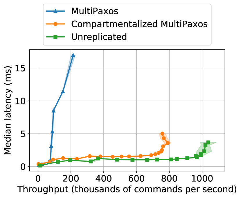
(b) With batching

Figure 28. The latency and throughput of MultiPaxos, Compartmentalized MultiPaxos, and an unreplicated state machine.

Experiment Description

We call MultiPaxos with the six compartmentalizations described in this paper Compartmentalized MultiPaxos. We implemented MultiPaxos, Compartmentalized MultiPaxos, and an unreplicated state machine in Scala using the Netty networking library (see github.com/mwhittaker/frankenpaxos). MultiPaxos employs $2f+1$ machines with each machine playing the role of a MultiPaxos proposer, acceptor, and replica. The unreplicated state machine is implemented as a single process on a single server. Clients send commands directly to the state machine. Upon receiving a command, the state machine executes the command and immediately sends back the result. Note that unlike MultiPaxos and Compartmentalized MultiPaxos, the unreplicated state machine is not fault tolerant. If the single server fails, all state is lost and no commands can be executed. Thus, the unreplicated state machine should not be viewed as an apples-to-apples comparison with the other two protocols. Instead, the unreplicated state machine sets an upper bound on attainable performance.

We measure the throughput and median latency of the three protocols under workloads with a varying numbers of clients. Each client issues state machine commands in a closed loop. It waits to receive the result of executing its most recently proposed command before it issues another. All three protocols replicate a key-value store state machine where the keys are integers and the values are 16 byte strings. In this benchmark, all state machine commands are writes. There are no reads.

We deploy the protocols with and without batching for $f=1$. Without batching, we deploy Compartmentalized MultiPaxos with two proposers, ten proxy leaders, a two by two grid of acceptors, and four replicas. With batching, we deploy two batchers, two proposers, three proxy replicas, a simple majority quorum system of three acceptors, two replicas, and three unbatchers. For simplicity, every node is deployed on its own machine, but in practice, nodes can be physically co-located. In particular, any two logical roles can be placed on the same machine without violating fault tolerance constraints, so long as the two roles are not the same.

We deploy the three protocols on AWS using a set of m5.xlarge machines within a single availability zone. Every m5.xlarge instance has 4 vCPUs and 16 GiB of memory. Everything is done in memory, and nothing is written to disk (because everything is replicated, data is persistent even without writing it to disk). In our experiments, the network is never a bottleneck. All numbers presented are the average of three executions of the benchmark. As is standard, we implement MultiPaxos and Compartmentalized MultiPaxos with thriftiness enabled (Moraru et al., 2013). For a given number of clients, the batch size is set empirically to optimize throughput. For a fair comparison, we deploy the unreplicated state machine with a set of batchers and unbatchers when batching is enabled.

Results

The results of the experiment are shown in Figure 28. The standard deviation of throughput measurements are shown as a shaded region. Without batching, MultiPaxos has a peak throughput of roughly 25,000 commands per second, while Compartmentalized MultiPaxos has a peak throughput of roughly 150,000 commands per second, a $6\times$ increase. The unreplicated state machine outperforms both protocols. It achieves a peak throughput of roughly 250,000 commands per second. Compartmentalized MultiPaxos underperforms the unreplicated state machine because—despite decoupling the leader as much as possible—the single leader remains a throughput bottleneck. Note that after fully compartmentalizing MultiPaxos, either the leader or the replicas are guaranteed to be the throughput bottleneck because all other components (e.g., proxy leaders, acceptors, batchers, unbatchers) can be scaled arbitrarily. Implementation and deployment details (e.g., what state machine is being replicated) determine which component is the ultimate throughput bottleneck. All three protocols have millisecond latencies at peak throughput. With batching, MultiPaxos, Compartmentalized MultiPaxos, and the unreplicated state machine have peak throughputs of roughly 200,000, 800,000 and 1,000,000 commands per second respectively.

Compartmentalized MultiPaxos uses $6.66\times$ more machines than MultiPaxos. On the surface, this seems like a weakness, but in reality it is a strength. MultiPaxos does not scale, so it is unable to take advantage of more machines. Compartmentalized MultiPaxos, on the other hand, achieves a $6\times$ increase in throughput using $6.66\times$ the number of resources. Thus, we achieve 90% of perfect linear scalability. In fact, with the mixed read-write workloads below, we are able to scale throughput superlinearly with the number of resources. This is because compartmentalization eliminates throughput bottlenecks. With throughput bottlenecks, non-bottlenecked components are underutilized. When we eliminate the bottlenecks, we eliminate underutilization and can increase performance without increasing the number of resources. Moreover, a protocol does not have to be fully compartmentalized. We can selectively compartmentalize some but not all throughput bottlenecks to reduce the number of resources needed. In other words, MultiPaxos and Compartmentalized MultiPaxos are not two alternatives, but rather two extremes in a trade-off between throughput and resource usage.

We also compared the unbatched performance of Compartmentalized MultiPaxos and the unreplicated state machine with values being 100 bytes and 1000 bytes. The results are shown in Figure 29. Expectedly, the protocols’ peak throughput decreases as we increase the value size.

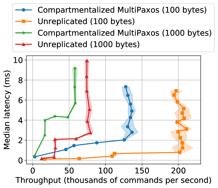
Figure 29. The latency and throughput of Compartmentalized MultiPaxos and an unreplicated state machine without batching and with larger value sizes.

8.2. Mencius Latency-Throughput

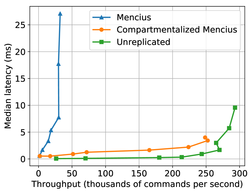
(a) Without batching

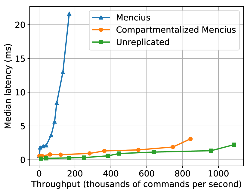
(b) With batching

Figure 30. The latency and throughput of Mencius, Compartmentalized Mencius, and an unreplicated state machine.

We repeat the experiment above but with Mencius and Compartmentalized Mencius. The results are shown in Figure 30. Without batching, Mencius can process roughly 30,000 commands per second. Compartmentalized Mencius can process roughly 250,000 commands per second, an $8.3\times$ improvement. With batching, Mencius and Compartmentalized Mencius achieve peak throughputs of nearly 200,000 and 850,000 commands per second respectively, a $4.25\times$ improvement.

8.3. S-Paxos Latency-Throughput

We repeat the experiments above with S-Paxos and Compartmentalized S-Paxos. Without batching, Compartmentalized S-Paxos achieves a peak throughput of 180,000 commands per second compared to S-Paxos’ throughput of 22,000 (an $8.2\times$ improvement). With batching, Compartmentalized S-Paxos achieves a peak throughput of 750,000 commands per second compared to S-Paxos’ throughput of 180,000 (a $4.16\times$ improvement). Note that our implementation of S-Paxos is not as optimized as our other two implementations, so its absolute performance is lower.

8.4. Ablation Study

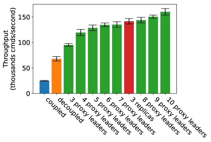
(a) Without batching

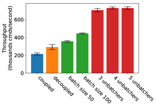
(b) With batching

Figure 31. An ablation study. Standard deviations are shown using error bars.

Experiment Description

We now perform an ablation study to measure the effect of each compartmentalization. In particular, we begin with MultiPaxos and then decouple and scale the protocol according to the six compartmentalizations, measuring peak throughput along the way. Note that we cannot measure the effect of each individual compartmentalization in isolation because decoupling and scaling a component only improves performance if that component is a bottleneck. Thus, to measure the effect of each compartmentalization, we have to apply them all, and we have to apply them in an order that is consistent with the order in which bottlenecks appear. All the details of this experiment are the same as the previous experiment unless otherwise noted.

Results

The unbatched ablation study results are shown in Figure 31(a). MultiPaxos has a throughput of roughly 25,000 commands per second. When we decouple the protocol and introduce proxy leaders (Section 3.1), we increase the throughput to roughly 70,000 commands per second. This decoupled MultiPaxos uses the bare minimum number of proposers (2), proxy leaders (2), acceptors (3), and replicas (2). We then scale up the number of proxy leaders from 2 to 7. The proxy leaders are the throughput bottleneck, so as we scale them up, the throughput of the protocol increases until it plateaus at roughly 135,000 commands per second. At this point, the proxy leaders are no longer the throughput bottleneck; the replicas are. We introduce an additional replica (Section 3.3), though the throughput does not increase. This is because proxy leaders broadcast commands to all replicas, so introducing a new replica increases the load on the proxy leaders making them the bottleneck again. We then increase the number of proxy leaders to 10 to increase the throughput to roughly 150,000 commands per second. At this point, we determined empirically that the leader was the bottleneck. In this experiment, the acceptors are never the throughput bottleneck, so increasing the number of acceptors does not increase the throughput (Section 3.2). However, this is particular to our write-only workload. In the mixed read-write workloads discussed momentarily, scaling up the number of acceptors is critical for high throughput.

The batched ablation study results are shown in Figure 31(b). We decouple MultiPaxos and introduce two batchers and two unbatchers with a batch size of 10 (Section 4.1, Section 4.2). This increases the throughput of the protocol from 200,000 commands per second to 300,000 commands per second. We then increase the batch size to 50 and then to 100. This increases throughput to 500,000 commands per second. We then increase the number of unbatchers to 3 and reach a peak throughput of roughly 800,000 commands per second. For this experiment, two batchers and three unbatchers are sufficient to handle the clients’ load. With more clients and a larger load, more batchers would be needed to maximize throughput.

Compartmentalization allows us to decouple and scale protocol components, but it doesn’t automatically tell us the extent to which we should decouple and scale. Understanding this, through ablation studies like the one presented here, must currently be done by hand. As a line of future work, we are researching how to automatically deduce the optimal amount of decoupling and scaling.

8.5. Read Scalability

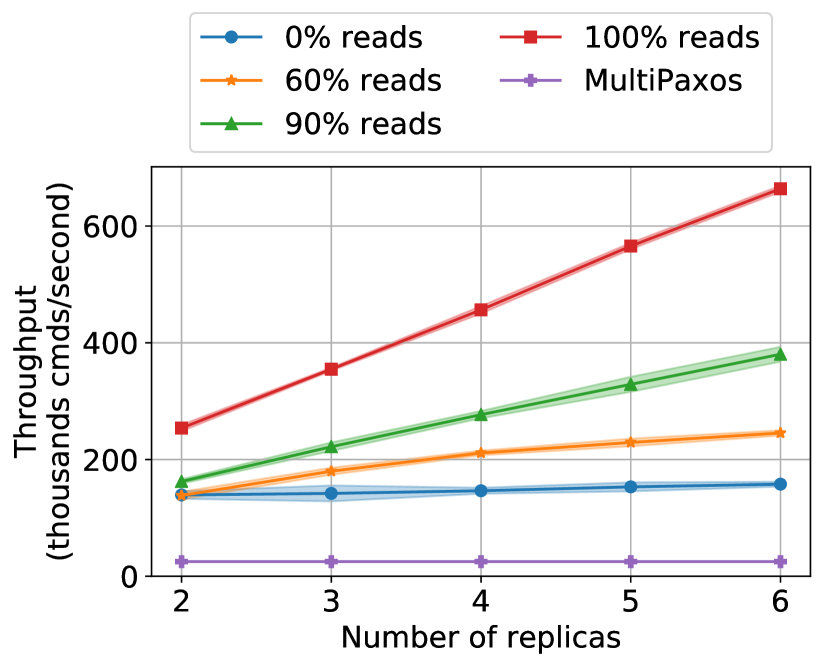
(a) Unbatched linearizable reads

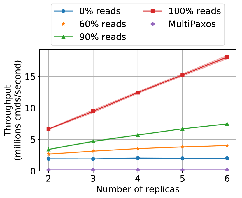
(b) Batched linearizable reads

Figure 32. Peak throughput vs the number of replicas

Experiment Description

Thus far, we have looked at write-only workloads. We now measure the throughput of Compartmentalized MultiPaxos under a workload with reads and writes. In particular, we measure how the throughput of Compartmentalized MultiPaxos scales as we increase the number of replicas. We deploy Compartmentalized MultiPaxos with and without batching; with 2, 3, 4, 5, and 6 replicas; and with workloads that have 0%, 60%, 90%, and 100% reads. For any given workload and number of replicas, proxy leaders, and acceptors is chosen to maximize throughput. The batch size is 50. In the batched experiments, we do not use batchers and unbatchers. Instead, clients form batches of commands themselves. This has no effect on the throughput measurements. We did this only to reduce the number of client machines that we needed to saturate the system. This was not an issue with the write-only workloads because they had significantly lower peak throughputs.

Results

The unbatched results are shown in Figure 32(a). We also show MultiPaxos’ throughput for comparison. MultiPaxos does not distinguish reads and writes, so there is only a single line to compare against. With a 0% read workload, Compartmentalized MultiPaxos has a throughput of roughly 150,000 commands per second, and the protocol does not scale much with the number of replicas. This is consistent with our previous experiments. For workloads with reads and writes, our results confirm two expected trends. First, the higher the fraction of reads, the higher the throughput. Second, the higher the fraction of reads, the better the protocol scales with the number of replicas. With a 100% read workload, for example, Compartmentalized MultiPaxos scales linearly up to a throughput of roughly 650,000 commands per second with 6 replicas. The batched results, shown in Figure 32(b), are very similar. With a 100% read workload, Compartmentalized MultiPaxos scales linearly up to a throughput of roughly 17.5 million commands per second.

Our results also show two counterintuitive trends. First, a small increase in the fraction of writes can lead to a disproportionately large decrease in throughput. For example, the throughput of the 90% read workload is far less than 90% of the throughput of the 100% read workload. Second, besides the 100% read workload, throughput does not scale linearly with the number of replicas. We see that the throughput of the 0%, 60%, and 90% read workloads scale sublinearly with the number of replicas. These results are not an artifact of our protocol; they are fundamental. Any state machine replication protocol where writes are processed by every replica and where reads are processed by a single replica (Terrace and Freedman, 2009; Zhu et al., 2019; Charapko et al., 2019) will exhibit these same two performance anomalies.

We can explain this analytically. Assume that we have $n$ replicas; that every replica can process at most $\alpha$ commands per second; and that we have a workload with a $f_{w}$ fraction of writes and a $f_{r}=1-f_{w}$ fraction of reads. Let $T$ be peak throughput, measured in commands per second. Then, our protocol has a peak throughput of $f_{w}T$ writes per second and $f_{r}T$ reads per second. Writes are processed by every replica, so we impose a load of $nf_{w}T$ writes per second on the replicas. Reads are processed by a single replica, so we impose a load of $f_{r}T$ reads per second on the replicas. The total aggregate throughput of the system is $n\alpha$, so we have $n\alpha=nf_{w}T+f_{r}T$. Solving for $T$, we find the peak throughput of our system is

$$\frac{n\alpha}{nf_{w}+f_{r}}$$

This formula is plotted in Figure 33 with $\alpha=100,000$. The limit of our peak throughput as $n$ approaches infinity is $\frac{\alpha}{f_{w}}$. This explains both of the performance anomalies described above. First, it shows that peak throughput has a $\frac{1}{f_{w}}$ relationship with the fraction of writes, meaning that a small increase in $f_{w}$ can have a large impact on peak throughput. For example, if we increase our write fraction from 1% to 2%, our throughput will half. A 1% change in write fraction leads to a 50% reduction in throughput. Second, it shows that throughput does not scale linearly with the number of replicas; it is upper bounded by $\frac{\alpha}{f_{w}}$. For example, a workload with 50% writes can never achieve more than twice the throughput of a 100% write workload, even with an infinite number of replicas.

The results for sequentially consistent and eventually consistent reads are shown in Figure 34. The throughput of these weakly consistent reads are similar to that of linearizable reads, but they can be performed with far fewer acceptors.

Figure 33. Analytical throughput vs the number of replicas.

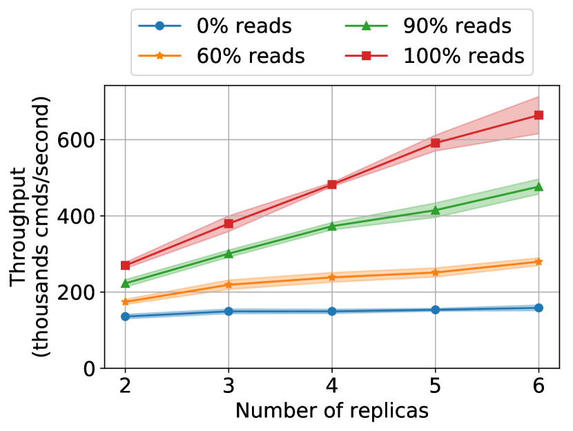
(a) Unbatched eventually consistent reads

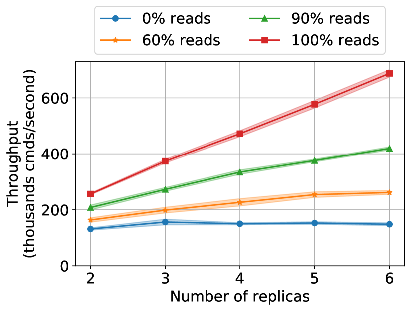
(b) Unbatched sequentially consistent reads

Figure 34. Peak throughput vs the number of replicas

8.6. Skew Tolerance

Experiment Description

CRAQ (Terrace and Freedman, 2009) is a chain replication (Van Renesse and Schneider, 2004) variant with scalable reads. A CRAQ deployment consists of at least $f+1$ nodes arranged in a linked list, or chain. Writes are sent to the head of the chain and propagated node-by-node down the chain from the head to the tail. When the tail receives the write, it sends a write acknowledgement to its predecessor, and this ack is propagated node-by-node backwards through the chain until it reaches the head. Reads are sent to any node. When a node receives a read of key $k$, it checks to see if it has any unacknowledged write to that key. If it doesn’t, then it performs the read and replies to the client immediately. If it does, then it forwards the read to the tail of the chain. When the tail receives a read, it executes the read immediately and replies to the client.

We now compare Compartmentalized MultiPaxos with our implementation of CRAQ. In particular, we show that CRAQ (and similar protocols like Harmonia (Zhu et al., 2019)) are sensitive to data skew, whereas Compartmentalized MultiPaxos is not. We deploy Compartmentalized MultiPaxos with two proposers, three proxy leaders, twelve acceptors, and six replicas, and we deploy CRAQ with six chain nodes. Though, our results hold for deployments with a different number of machines as well, as long as the number of Compartmentalized MultiPaxos replicas is equal to the number of CRAQ chain nodes. Both protocols replicate a key-value store with 10,000 keys in the range $1,\ldots,10,000$. We subject both protocols to the following workload. A client repeatedly flips a weighted coin, and with probability $p$ chooses to read or write to key $0$. With probability $1-p$, it decides to read or write to some other key $2,\ldots,10,000$ chosen uniformly at random. The client then decides to perform a read with 95% probability and a write with 5% probability. As we vary the value of $p$, we vary the skew of the workload. When $p=0$, the workload is completely uniform, and when $p=1$, the workload consists of reads and writes to a single key. This artificial workload allows to study the effect of skew in a simple way without having to understand more complex skewed distributions.

Results

The results are shown in Figure 35, with $p$ on the $x$-axis. The throughput of Compartmentalized MultiPaxos is constant; it is independent of $p$. This is expected because Compartmentalized MultiPaxos is completely agnostic to the state machine that it is replicating and is completely unaware of the notion of keyed data. Its performance is only affected by the ratio of reads to writes and is completely unaffected by what data is actually being read or written. CRAQ, on the other hand, is susceptible to skew. As we increase skew from $p=0$ to $p=1$, the throughput decreases from roughly 300,000 commands per second to roughly 100,000 commands per second. As we increase $p$, we increase the fraction of reads which are forwarded to the tail. In the extreme, all reads are forwarded to the tail, and the throughput of the protocol is limited to that of a single node (i.e. the tail).

However, with low skew, CRAQ can perform reads in a single round trip to a single chain node. This allows CRAQ to implement reads with lower latency and with fewer nodes than Compartmentalized MultiPaxos. However, we also note that Compartmentalized MultiPaxos outperforms CRAQ in our benchmark even with no skew. This is because every chain node must process four messages per write, whereas Compartmentalized MultiPaxos replicas only have to process two. CRAQ’s write latency also increases with the number of chain nodes, creating a hard trade-off between read throughput and write latency. Ultimately, neither protocol is strictly better than the other. For very read-heavy workloads with low-skew, CRAQ will likely outperform Compartmentalized MultiPaxos using fewer machines, and for workloads with more writes or more skew, Compartmentalized MultiPaxos will likely outperform CRAQ. For the 95% read workload in our experiment, Compartmentalized MultiPaxos has strictly better throughput than CRAQ across all skews, but this is not true for workloads with a higher fraction of reads.

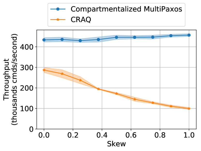
Figure 35. The effect of skew on Compartmentalized MultiPaxos and CRAQ.

8.7. Comparison to Scalog

Experiment Description

Scalog (Ding et al., 2020) is a replicated shared log protocol that achieves high throughput using an idea similar to Compartmentalized MultiPaxos’ batchers and unbatchers. We implemented Scalog to compare against Compartmentalized MultiPaxos with batching, but the two protocols are not immediately comparable. Scalog is replicated shared log protocol, whereas Compartmentalized MultiPaxos is a state machine replication protocol. Practically, the main difference between the two is that Scalog doesn’t have state machine replicas. To compare the two protocols fairly, we extended Scalog with replicas to implement state machine replication.

For simplicity, we implemented Scalog with a single aggregator, though we confirmed empirically that it was never the bottleneck. We deploy Scalog with three shards, two servers per shard, and five replicas. Servers send their local cuts to the aggregator after every 100 commands received. Re-running the same experiment from Section 8.1, we measure the latency and throughput of the protocol on a write-only workload as we vary the number of clients.

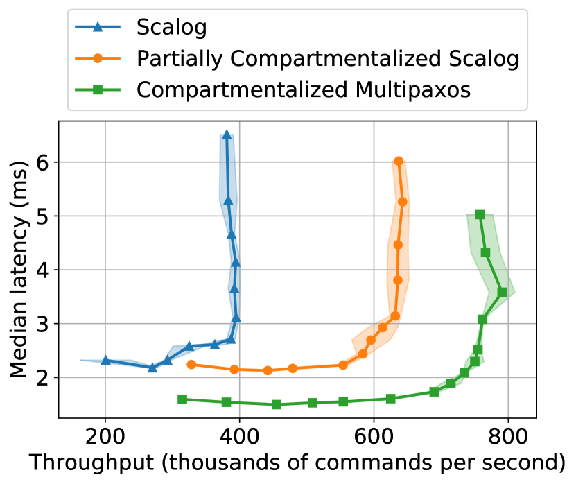
Figure 36. The latency and throughput of Scalog, Compartmentalized Scalog, and Compartmentalized MultiPaxos.

Results

The results are shown in Figure 36. Scalog achieves a peak throughput of roughly 400,000 commands per second compared to Compartmentalized MultiPaxos’ throughput of 800,000 commands per second. Scalog also uses 17 machines, and Compartmentalized MultiPaxos uses 15. The Scalog servers implement batching very efficiently, however, batching is not the bottleneck in our experiment. The protocol is instead bottlenecked by the replicas. This demonstrates the importance of eliminating every bottleneck rather than eliminating a single bottleneck. We compartmentalized the Scalog replicas by introducing proxy replicas. When deployed with two replicas and four proxy replicas, the protocol’s throughput increased to roughly 650,000 requests per second. This is a $1.625\times$ increase in throughput using one additional machine (a $1.05\times$ increase in the number of machines).

9. Related Work

MultiPaxos

Unlike state machine replication protocols like Raft (Ongaro and Ousterhout, 2014) and Viewstamped Replication (Liskov and Cowling, 2012), MultiPaxos (Lamport, 1998, 2001; Van Renesse and Altinbuken, 2015) is designed with the roles of proposer, acceptor, and replicas logically decoupled. This decoupling alone is not sufficient for MultiPaxos to achieve the best possible throughput, but the decoupling allows for the compartmentalizations described in this paper.

PigPaxos

PigPaxos (Charapko et al., 2020) is a MultiPaxos variant that alters the communication flow between the leader and the acceptors to improve scalability and throughput. Similar to compartmentalization, PigPaxos realizes that the leader is doing many different jobs and is a bottleneck in the system. In particular, PigPaxos substitutes direct leader-to-acceptor communication with a relay network. In PigPaxos the leader sends a message to one or more randomly selected relay nodes, and each relay rebroadcasts the leader’s message to the peers in its relay-group and waits for some threshold of responses. Once each relay receives enough responses from its peers, it aggregates them into a single message to reply to the leader. The leader selects a new set of random relays for each new message to prevent faulty relays from having a long-term impact on the communication flow. PigPaxos relays are comparable to our proxy leaders, although the relays are simpler and only alter the communication flow. As such, the relays cannot generally take over the other leader roles, such as quorum counting or replying to the clients. Unlike PigPaxos, whose main goal is to grow to larger clusters, compartmentalization is more general and improves throughput under different conditions and situations.

Chain Replication

Chain Replication (Van Renesse and Schneider, 2004) is a state machine replication protocol in which the set of state machine replicas are arranged in a totally ordered chain. Writes are propagated through the chain from head to tail, and reads are serviced exclusively by the tail. Chain Replication has high throughput compared to MultiPaxos because load is more evenly distributed between the replicas, but every replica must process four messages per command, as opposed to two in Compartmentalized MultiPaxos. The tail is also a throughput bottleneck for read-heavy workloads. Finally, Chain Replication is not tolerant to network partitions and is therefore not appropriate in all situations.

Ring Paxos

Ring Paxos (Marandi et al., 2010) is a MultiPaxos variant that decouples control flow from data flow (as in S-Paxos (Biely et al., 2012)) and that arranges nodes in a chain (as in Chain Replication). As a result, Ring Paxos has the same advantages as S-Paxos and Chain Replication. Like S-Paxos and Mencius, Ring Paxos eliminates some but not all throughput bottlenecks. It also does not optimize reads; reads are processed the same as writes.

NoPaxos

NoPaxos (Li et al., 2016) is a Viewstamped Replication (Liskov and Cowling, 2012) variant that depends on an ordered unreliable multicast (OUM) layer. Each client sends commands to a centralized sequencer that is implemented on a network switch. The sequencer assigns increasing IDs to the commands and broadcasts them to a set of replicas. The replicas speculatively execute commands and reply to clients. In this paper, we describe how to use proxy leaders to avoid having a centralized leader. NoPaxos’ on-switch sequencer is a hardware based alternative to avoid the bottleneck.

Scalog

Scalog (Ding et al., 2020) is a replicated shared log protocol that achieves high throughput using an idea similar to Compartmentalized MultiPaxos’ batchers and unbatchers. A client does not send values directly to a centralized leader for sequencing in the log. Instead, the client sends its values to one of a number of servers. Periodically, the servers’ batches are sealed and assigned an id. This id is then sent to a state machine replication protocol, like MultiPaxos, for sequencing.

Compartmentalization and Scalog are fundamentally different because compartmentalization is a generally applicable technique, while Scalog is a protocol. Because compartmentalization is a technique, it can be applied to many existing protocols. In this paper, we have shown how to compartmentalize MultiPaxos, Mencius, and S-Paxos. In (Whittaker et al., 2020), we show how to compartmentalize EPaxos (Moraru et al., 2013). In Section 8.7, we even show how to partially compartmentalize Scalog. Scalog, on the other hand, is a specific protocol.

Restricting our attention to Compartmentalized MultiPaxos, Scalog and Compartmentalized MultiPaxos are still fundamentally different. Scalog is a log replication protocol, whereas Compartmentalized MultiPaxos is a complete state machine replication protocol. In other words, Scalog doesn’t have state machine replicas, while Compartmentalized MultiPaxos does. These two types of protocols are similar, but differ in a number of key ways. For example, to implement state machine replication on top of Scalog, we have to implement the replicas ourselves, and as discussed in Section 8.7, these replicas become the protocol’s throughput bottleneck when they’re not compartmentalized. As an another example, Scalog cannot perform fast linearizable reads like Compartmentalized MultiPaxos can, as described in Section 3.4.

Ignoring this, the two protocols still have different focuses. Scalog focuses on one bottleneck. Specifically, the protocol implements an efficient form of batching, with a focus on replicating commands before ordering them. Compartmentalized MultiPaxos, on the other hand, provides a framework to address every bottleneck. Compartmentalized batchers solve the same problem as Scalog servers, and the introduction of proxy leaders, flexible quorums, unbatchers, decoupled read and write paths addresses the other bottlenecks that we have seen arise. Scalog does not address these other bottlenecks. We show this empirically in Section 8.7. This is a contribution of our paper.

There are other technical differences between the two protocols as well. For example, there is complexity in managing the Scalog aggregators. If one fails, we need to detect and replace it. If the root fails, for example, the short term “goodput” drops to zero. Moreover, if a Compartmentalized batcher in Compartmentalized MultiPaxos fails, we lose all of its unsent commands. If any server in a Scalog shard fails, then any unreplicated commands on any of the servers within the shard are lost.

Scalable Agreement

In (Kapritsos and Junqueira, 2010), Kapritsos et al. present a protocol similar to Compartmentalized Mencius. The protocol round-robin partitions log entries among a set of replica clusters co-located on a fixed set of machines. Every cluster has $2f+1$ replicas, with every replica playing the role of a Paxos proposer and acceptor. Compartmentalized Mencius extends the protocol with the compartmentalizations described in this paper.

SEDA Architecture

The SEDA architecture (Welsh et al., 2001) is a server architecture in which functionality is divided into a pipeline of multithreaded modules that communicate with one another using queues. This architecture introduces pipeline parallelism and allows individual components to be scaled up or down to avoid becoming the bottleneck. Our work on decoupling and scaling state machine replication protocols borrows these same ideas, except that we apply them at a fine grain to distributed protocols rather than a single server.

Multithreaded Replication

(Santos and Schiper, 2013a) and (Behl et al., 2015) both propose multithreaded state machine replication protocols. The protocol in (Santos and Schiper, 2013a) is implemented using a combination of actors and the SEDA architecture (Welsh et al., 2001). A replica’s functionality is decoupled into a number of modules, with each module run on its own thread. For example, a MultiPaxos leader has one module to receive messages, one to sequence them, and one to send them. (Behl et al., 2015) argues for a Mencius-like approach in which each thread has complete functionality (receiving, sequencing, and sending), with slots round-robin partitioned across threads. Multithreaded protocols like these are necessarily decoupled and scale within a single machine. This work is complementary to compartmentalization. Compartmentalization works at the protocol level, while multithreading works on the process level. Both can be applied to a single protocol.

A Family of Leaderless Generalized Protocols

In (Losa et al., 2016), Losa et al. propose a template that can be used to implement state machine replication protocols that are both leaderless and generalized. The template involves a module to compute dependencies between commands and a module to choose and execute commands. The goal of this modularization is to unify existing protocols like EPaxos (Moraru et al., 2013), and Caesar (Arun et al., 2017). However, the modularity also introduces decoupling which can lead to performance gains. This is an example of compartmentalization.

Read Leases

A common way to optimize reads in MultiPaxos is to grant a lease to the leader (Chandra et al., 2007; Corbett et al., 2013; Burrows, 2006). While the leader holds the lease, no other node can become leader. As a result, the leader can perform reads locally without contacting other nodes. Leases assume some degree of clock synchrony, so they are not appropriate in all circumstances. Moreover, the leader is still a read bottleneck. Raft has a similar optimization that does not require any form of clock synchrony, but the leader is still a read bottleneck (Ongaro and Ousterhout, 2014). With Paxos Quorum Leases (Moraru et al., 2014), any set of nodes—not just the leader—can hold a lease for a set of objects. These lease holders can read the objects locally. Paxos Quorum Leases assume clock synchrony and are a special case of Paxos Quorum Reads (Charapko et al., 2019) in which read quorums consist of any lease holding node and write quorums consist of any majority that includes all the lease holding nodes. Compartmentalization MultiPaxos does not assume clock synchrony and has no read bottlenecks.

Harmonia

Harmonia (Zhu et al., 2019) is a family of state machine replication protocols that leverage specialized hardware—specifically, a specialized network switch—to achieve high throughput and low latency. Like CRAQ, Harmonia is sensitive to data skew. It performs extremely well under low contention, but degrades in performance as contention grows. Harmonia also assumes clock synchrony, whereas Compartmentalized MultiPaxos does not. FLAIR (Takruri et al., 2020) is replication protocol that also leverages specialized hardware, similar to Harmonia.

Sharding

In this paper, we have discussed state machine replication in its most general form. We have not made any assumptions about the nature of the state machines themselves. Because of this, we are not able to decouple the state machine replicas. Every replica must execute every write. This creates a fundamental throughput limit. However, if we are able to divide the state of the state machine into independent shards, then we can further scale the protocols by sharding the state across groups of replicas. For example, in (Bezerra et al., 2014), Bezerra et al. discuss how state machine replication protocols can take advantage of sharding.

Low Latency Replication Protocols

While compartmentalization increases throughput, it also increases the number of network delays required to get a state machine command executed. For example, starting from a client, MultiPaxos can execute a state machine command and return a response to a client in four network delays, whereas Compartmentalized MultiPaxos requires six. Within a single data center, this translates to a small increase in latency, but when deployed on a wide area network, the latency is increased substantially. Thus, if your goal is to minimize latency, you should choose latency optimized protocols like CURP (Park and Ousterhout, 2019) or SpecPaxos (Ports et al., 2015) over a compartmentalized protocol.

10. Conclusion

In this paper, we analyzed the throughput bottlenecks in state machine replication protocols and demonstrated how to eliminate them using a combination of decoupling and scale, a technique we call compartmentalization. Using compartmentalization, we establish a new baseline for MultiPaxos’ performance. We increase the protocol’s throughput by a factor of $6\times$ on a write-only workload and $16\times$ on a 90% read workload, all without the need for complex or specialized protocols.

References

- (1)
- tid ([n.d.]) [n.d.]. A Brief Introduction of TiDB. https://pingcap.github.io/blog/2017-05-23-perconalive17/. Accessed: 2019-10-21.
- cos ([n.d.]) [n.d.]. Global data distribution with Azure Cosmos DB - under the hood. https://docs.microsoft.com/en-us/azure/cosmos-db/global-dist-under-the-hood. Accessed: 2019-10-21.
- cas ([n.d.]) [n.d.]. Lightweight transactions in Cassandra 2.0. https://www.datastax.com/blog/2013/07/lightweight-transactions-cassandra-20. Accessed: 2019-10-21.
- yug ([n.d.]) [n.d.]. Raft Replication in YugaByte DB. https://www.yugabyte.com/resources/raft-replication-in-yugabyte-db/. Accessed: 2019-10-21.
- Ailijiang et al. (2019) Ailidani Ailijiang, Aleksey Charapko, Murat Demirbas, and Tevfik Kosar. 2019. WPaxos: Wide Area Network Flexible Consensus. IEEE Transactions on Parallel and Distributed Systems (2019).
- Arun et al. (2017) Balaji Arun, Sebastiano Peluso, Roberto Palmieri, Giuliano Losa, and Binoy Ravindran. 2017. Speeding up Consensus by Chasing Fast Decisions. In Dependable Systems and Networks (DSN), 2017 47th Annual IEEE/IFIP International Conference on. IEEE, 49–60.
- Atikoglu et al. (2012) Berk Atikoglu, Yuehai Xu, Eitan Frachtenberg, Song Jiang, and Mike Paleczny. 2012. Workload analysis of a large-scale key-value store. In Proceedings of the 12th ACM SIGMETRICS/PERFORMANCE joint international conference on Measurement and Modeling of Computer Systems. 53–64.
- Behl et al. (2015) Johannes Behl, Tobias Distler, and Rüdiger Kapitza. 2015. Consensus-oriented parallelization: How to earn your first million. In Proceedings of the 16th Annual Middleware Conference. ACM, 173–184.
- Bezerra et al. (2014) Carlos Eduardo Bezerra, Fernando Pedone, and Robbert Van Renesse. 2014. Scalable state-machine replication. In 2014 44th Annual IEEE/IFIP International Conference on Dependable Systems and Networks. IEEE, 331–342.
- Biely et al. (2012) Martin Biely, Zarko Milosevic, Nuno Santos, and Andre Schiper. 2012. S-paxos: Offloading the leader for high throughput state machine replication. In Reliable Distributed Systems (SRDS), 2012 IEEE 31st Symposium on. IEEE, 111–120.
- Burrows (2006) Mike Burrows. 2006. The Chubby lock service for loosely-coupled distributed systems. In Proceedings of the 7th symposium on Operating systems design and implementation. USENIX Association, 335–350.
- Chandra et al. (2007) Tushar D Chandra, Robert Griesemer, and Joshua Redstone. 2007. Paxos made live: an engineering perspective. In Proceedings of the twenty-sixth annual ACM symposium on Principles of distributed computing. ACM, 398–407.
- Charapko et al. (2019) Aleksey Charapko, Ailidani Ailijiang, and Murat Demirbas. 2019. Linearizable quorum reads in Paxos. In 11th USENIX Workshop on Hot Topics in Storage and File Systems (HotStorage 19).
- Charapko et al. (2020) Aleksey Charapko, Ailidani Ailijiang, and Murat Demirbas. 2020. PigPaxos: Devouring the communication bottlenecks in distributed consensus. arXiv preprint arXiv:2003.07760 (2020).
- Corbett et al. (2013) James C Corbett, Jeffrey Dean, Michael Epstein, Andrew Fikes, Christopher Frost, Jeffrey John Furman, Sanjay Ghemawat, Andrey Gubarev, Christopher Heiser, Peter Hochschild, et al. 2013. Spanner: Google’s globally distributed database. ACM Transactions on Computer Systems (TOCS) 31, 3 (2013), 8.
- Ding et al. (2020) Cong Ding, David Chu, Evan Zhao, Xiang Li, Lorenzo Alvisi, and Robbert van Renesse. 2020. Scalog: Seamless Reconfiguration and Total Order in a Scalable Shared Log. In 17th USENIX Symposium on Networked Systems Design and Implementation (NSDI 20). 325–338.
- Ghemawat et al. (2003) Sanjay Ghemawat, Howard Gobioff, and Shun-Tak Leung. 2003. The Google file system. In Proceedings of the nineteenth ACM symposium on Operating systems principles. 29–43.
- Herlihy and Wing (1990) Maurice P Herlihy and Jeannette M Wing. 1990. Linearizability: A correctness condition for concurrent objects. ACM Transactions on Programming Languages and Systems (TOPLAS) 12, 3 (1990), 463–492.
- Howard et al. (2017) Heidi Howard, Dahlia Malkhi, and Alexander Spiegelman. 2017. Flexible Paxos: Quorum Intersection Revisited. In 20th International Conference on Principles of Distributed Systems (OPODIS 2016) (Leibniz International Proceedings in Informatics (LIPIcs)), Panagiota Fatourou, Ernesto Jiménez, and Fernando Pedone (Eds.), Vol. 70. Schloss Dagstuhl–Leibniz-Zentrum fuer Informatik, Dagstuhl, Germany, 25:1–25:14. https://doi.org/10.4230/LIPIcs.OPODIS.2016.25
- Jin et al. (2018) Xin Jin, Xiaozhou Li, Haoyu Zhang, Nate Foster, Jeongkeun Lee, Robert Soulé, Changhoon Kim, and Ion Stoica. 2018. Netchain: Scale-free sub-rtt coordination. In 15th USENIX Symposium on Networked Systems Design and Implementation (NSDI 18). 35–49.
- Kapritsos and Junqueira (2010) Manos Kapritsos and Flavio Paiva Junqueira. 2010. Scalable Agreement: Toward Ordering as a Service.. In HotDep.
- Lamport (1979) Leslie Lamport. 1979. How to make a multiprocessor computer that correctly executes multiprocess progranm. IEEE transactions on computers 9 (1979), 690–691.
- Lamport (1998) Leslie Lamport. 1998. The part-time parliament. ACM Transactions on Computer Systems (TOCS) 16, 2 (1998), 133–169.
- Lamport (2001) Leslie Lamport. 2001. Paxos made simple. ACM Sigact News 32, 4 (2001), 18–25.
- Lamport (2005) Leslie Lamport. 2005. Generalized consensus and Paxos. (2005).
- Lamport (2006) Leslie Lamport. 2006. Fast paxos. Distributed Computing 19, 2 (2006), 79–103.
- Lamport (2019) Leslie Lamport. 2019. Time, clocks, and the ordering of events in a distributed system. In Concurrency: the Works of Leslie Lamport. 179–196.
- Li et al. (2016) Jialin Li, Ellis Michael, Naveen Kr Sharma, Adriana Szekeres, and Dan RK Ports. 2016. Just Say NO to Paxos Overhead: Replacing Consensus with Network Ordering. In 12th USENIX Symposium on Operating Systems Design and Implementation (OSDI 16). 467–483.
- Liskov and Cowling (2012) Barbara Liskov and James Cowling. 2012. Viewstamped replication revisited. (2012).
- Losa et al. (2016) Giuliano Losa, Sebastiano Peluso, and Binoy Ravindran. 2016. Brief announcement: A family of leaderless generalized-consensus algorithms. In Proceedings of the 2016 ACM Symposium on Principles of Distributed Computing. ACM, 345–347.
- Mao et al. (2008) Yanhua Mao, Flavio P Junqueira, and Keith Marzullo. 2008. Mencius: building efficient replicated state machines for WANs. In 8th USENIX Symposium on Operating Systems Design and Implementation (OSDI 08). 369–384.
- Marandi et al. (2010) Parisa Jalili Marandi, Marco Primi, Nicolas Schiper, and Fernando Pedone. 2010. Ring Paxos: A high-throughput atomic broadcast protocol. In 2010 IEEE/IFIP International Conference on Dependable Systems & Networks (DSN). IEEE, 527–536.
- Moraru et al. (2013) Iulian Moraru, David G Andersen, and Michael Kaminsky. 2013. There is more consensus in egalitarian parliaments. In Proceedings of the Twenty-Fourth ACM Symposium on Operating Systems Principles. ACM, 358–372.
- Moraru et al. (2014) Iulian Moraru, David G Andersen, and Michael Kaminsky. 2014. Paxos quorum leases: Fast reads without sacrificing writes. In Proceedings of the ACM Symposium on Cloud Computing. 1–13.
- Nishtala et al. (2013) Rajesh Nishtala, Hans Fugal, Steven Grimm, Marc Kwiatkowski, Herman Lee, Harry C Li, Ryan McElroy, Mike Paleczny, Daniel Peek, Paul Saab, et al. 2013. Scaling memcache at facebook. In Presented as part of the 10th USENIX Symposium on Networked Systems Design and Implementation (NSDI 13). 385–398.
- Ongaro and Ousterhout (2014) Diego Ongaro and John K Ousterhout. 2014. In search of an understandable consensus algorithm.. In USENIX Annual Technical Conference. 305–319.
- Park and Ousterhout (2019) Seo Jin Park and John Ousterhout. 2019. Exploiting commutativity for practical fast replication. In 16th USENIX Symposium on Networked Systems Design and Implementation (NSDI 19). 47–64.
- Ports et al. (2015) Dan RK Ports, Jialin Li, Vincent Liu, Naveen Kr Sharma, and Arvind Krishnamurthy. 2015. Designing Distributed Systems Using Approximate Synchrony in Data Center Networks.. In NSDI. 43–57.
- Santos and Schiper (2012) Nuno Santos and André Schiper. 2012. Tuning paxos for high-throughput with batching and pipelining. In International Conference on Distributed Computing and Networking. Springer, 153–167.