The Role of Referrals in Immobility, Inequality, and Inefficiency in Labor Markets

Abstract

We study the consequences of job markets’ heavy reliance on referrals. Referrals screen candidates and lead to better matches and increased productivity, but disadvantage job-seekers who have few or no connections to employed workers, leading to increased inequality. Coupled with homophily, referrals also lead to immobility: a demographic group’s low current employment rate leads that group to have relatively low future employment as well. We identify conditions under which distributing referrals more evenly across a population not only reduces inequality, but also improves future productivity and economic mobility. We use the model to examine optimal policies, showing that one-time affirmative action policies involve short-run production losses, but lead to long-term improvements in equality, mobility, and productivity due to induced changes in future referrals. We also examine how the possibility of firing workers changes the effects of referrals.

JEL Classification Codes: D85, D13, L14, O12, Z13

Keywords: Inequality, Immobility, Job Contacts, Job Referrals, Social Networks, Networks, Productivity

I’ve never seen baseball advertise for a job, and I’ve never heard of whites applying for a job. I mean, there’s an old boy network, and it’s lily white. Frank Robinson

1 Introduction

The past few decades have seen inequality in countries like the US and UK rise to levels not seen since the Great Depression, and witnessed countries like China hit unprecedented levels of inequality. Inequality within a generation is accompanied by immobility across generations, as made clear by Alan Krueger’s 2012 famous demonstration of the “Great Gatsby Curve,” which showed that countries with higher inequality also tend to have higher immobility (a correlation between parent and child income). Understanding the common sources of inequality and immobility is essential to designing policies that deal not only with their symptoms but also their causes.

Some forces underlying persistent inequality and immobility – such as prejudice, racism, and cultural features like caste systems – are based on biases in people’s treatment and expectations of others. Other forces are structural – in the ways that markets work – and can lead to persistent differences even in the absence of any behavioral biases. Both need to be understood and addressed to improve welfare. Here we study a central form of structural bias in markets that leads to persistent inequality, immobility and inefficiency in markets, and policies to mitigate the bias. Most importantly, there is broad evidence that network connections lead to substantial differences in employment across people. For instance, Laschever (2013) uses random assignments to military units to show a forty percent spillover in peers’ employment years later.

A key feature of labor markets is that many, if not most, employees – of all skill levels – are hired via referrals, and people applying without some connection are at a substantial disadvantage. Furthermore these connections typically exhibit a degree of group-based homophily – the tendency of people to be friends with others with similar characteristics: ethnicity, gender, age, religion, etc. This homophily distorts the distribution of referrals in the population as a whole and has implications for inequality, immobility and productivity.

In this paper we develop a model in which current employees refer new ones. These referrals exhibit homophily, so that employees are more likely to refer workers of their own race, geneder, etc. Firms hire both via referrals and open applications. This allows us to provide a detailed analysis of the role of referrals in driving inequality and the persistence of that inequality (immobility), as well as the impact on productivity. The model also enables us to study the dynamic impacts of key policies: the short and long-term effects of different forms of affirmative action, as well as how hiring from open applications is affected by the ease with which firms can identify and fire workers who underperform.

The effect of referrals on inequality is well known. In particular, the reliance on referrals can result in inequality in employment and wages across groups. For instance, in our model, referred workers have an advantage of extra chances of being hired, and higher average wages conditional upon being hired, since their value is known and they are being selected for that higher value.

What has not been analyzed is the relationship between referrals and immobility as well as productivity, and the role of homophily in all three relationships. In particular, homophily coupled with referrals also helps us understand why inequality is so strongly tied with immobility. If one is born into a group that has poor employment, and has most of their connections within that group, then it becomes hard to get referrals to jobs. Thus, when there is high inequality across groups, referrals can make it naturally persistent. Referrals also serve a productive purpose. Namely, referrals provide information about the productivity of referred workers. Referrals thus help firms vet workers, and hence those hired via referrals are more productive (according to several measurements), on average, than those hired through a less informative open application process. Asymmetric distributions of referrals, which result from homophily when employment rates across groups are not balanced, mean that fewer workers with high productivities are being found and employed, and so again we see the role of homophily and referrals.

In summary, comparing an economy in which referrals are spread widely to one in which they are concentrated among a subset of a society not only leads to increased inequality and immobility, but also lowers a society’s productivity. Thus, inequality in employment and wages is not only to be related to immobility, but also to lower productivity. Although the intuitions behind these relationships are straightforward, the details are not, since the structure of equilibria and their dynamics involve countervailing effects and nontrivial analysis, as we discuss more below.

Another key focus of our study is to examine policies in this sort of market, including different forms of affirmative action. The first class of policies we consider – affirmative action policies – boil down to influencing the relative fractions of workers hired from under-represented groups (greens) and over-represented groups (blues). Roughly, this can be done in two ways: encouraging the hiring of referred greens who normally would have been rejected, or else discouraging the hiring of some blues from referrals so that more greens without a connection have a chance to be hired.

We show two main results on the economic impact of affirmative action policies. First, while affirmative action is usually analyzed in terms of short-run implications, we show that affirmative action has long-lasting implications for inequality, immobility, and productivity. The basic intuition is that it helps even the distribution of referrals, and that this network effect then persists across generations. This offers an explanation as to why data show that affirmative action has a lasting effect, even after it is removed. By bringing the balance of blue and green employment into better alignment with their prevalence in the population, the concentration of future referrals is reduced. This not only reduces current inequality, but also reduces immobility and bolsters future productivity. Second, discouraging the hiring of referred blues versus encouraging the hiring of referred greens involve different productivity impacts. Which policy involves less current loss of productivity depends on the composition of workers applying via open applications (either because they do not have a referral or because they were not hired through their referral) . When workers applying via open applications have a high expected productivity and are likely to be green, then it is better to discourage the hiring of referred blues in favor of those applying via open applications, while if the expected productivity is low and workers applying via open applications are unlikely to be green, then it is better to encourage the hiring of (low-productivity) referred greens. Furthermore, subject to feasibility, it is always better to pursue one of these policies rather than a mixture of the two.

Thus our analysis provides new insights about the longevity of affirmative action policies, as well as how the different ways in which it can be implemented have different short-term consequences.

We also consider another policy, which involves an extension to the structure of the model. In our basic model, once a worker is hired, then the firm retains with that worker for the next full period. In an extension, we consider what happens when firms can fire workers part way through a period. The ability to fire a worker improves the market by making it relatively more attractive for a firm to hire workers applying via open applications, since the firm can get rid of a low productivity worker should it end up hiring one, and get a second try at hiring. This improvement of the efficiency of hiring applying via open applications ends up improving productivity, and also lowering inequality and immobility.

Lastly, we study the effects of changes in macroeconomic conditions on inequality and inefficiency. Reducing the number of firms hiring leads to a reduction in production. However, the remaining firms are better able to secure high-skilled workers so that labor productivity (per worker) increases. This reduced competition in hiring also depresses wages as fewer firms are competing for the same workers.

Our analysis is nuanced and more complicated than initial intuitions would suggest. The main challenges are twofold.

First, there are two different ways in which referrals can be concentrated, and each has different effects. To understand this distinction it is important to note that more than one current employee might refer the same person. For instance, if blues have a higher employment rate than greens, and tend to refer other blues, then as the current employment becomes more tilted towards blues, more blues will get referrals and fewer greens will – with more blues getting multiple referrals. This corresponds to one way in which referrals can be concentrated, which is to have a smaller number of the next generation get referrals. Given that referrals provide information, firms have information about fewer applicants, which hurts overall productivity. Thus, it is this sort of concentration that is the key to understanding the impact of changing the distribution of referrals on productivity.

In contrast, to understand inequality in wages, one needs to understand the effects of multiple referrals. Having more than one referral can give an employee multiple offers and hence more bargaining power. Thus, determining the fraction of the population that gets higher wages as referrals are concentrated depends on the fraction of the population that gets multiple referrals. Note that increasing the probability of not getting a referral is neither necessary nor sufficient for having a larger fraction of the population get multiple referrals. Since how many people get any referral governs productivity and how many people get multiple referrals drives wage inequality, there is a close but imperfect relationship between how productivity and inequality are influenced by referrals.

Second, beyond the direct effect that referrals have on who gets employment offers, referrals also have an indirect countervailing effect – a lemons effect – that makes comparative statics regarding the impacts of referrals somewhat subtle. The lemons effect refers to the phenomenon that some people who apply for jobs via open applications had referrals but were not hired via those referrals – so they were already rejected by at least one firm. The fact that the open applications include previously-rejected job seekers lowers the expected productivity from hiring via open applications. A main complication in our analysis is that the lemons effect decreases as one concentrates referrals, since there are then fewer workers who are screened by hiring firms and rejected. This effect attenuates the relationship between productivity and the concentration of referrals. It also complicates the relationship between inequality and the concentration of referrals, and causes comparative statics on inequality to differ fundamentally from the comparative statics on productivity. All of our results, and their proofs, deal with this issue.

The rest of the paper is organized as follows. In Section 2, we introduce the model and discuss how the aggregate distribution of referrals determines hiring decisions, wages, and productivity. In Section 3, we introduce groups of agents – e.g., tracking ethnicity or gender – to follow employment of different groups and see how referrals link group outcomes over generations (immobility) and generate inefficiency. We then proceed, in Section 4, to study interventions, such as affirmative action policies. Such interventions have long-lasting effects, and even one time interventions not only reduce short-term inequality, but also increase mobility and improving efficiency for generations to come. In Section 5 we study the effects of changes in the referral distribution on population-wide measures of inequality and productivity. We also identify the different aspects of the referral distribution that determine productivity, inequality and immobility. While logically distinct, we show how these different aspects are jointly determined so that referrals tie together productivity, inequality and immobility. We also examine how productivity and wages vary with the number of firms hiring. Section 6 concludes.

More Discussion of the Relationship to the Literature.

As discussed in the many references mentioned above, it is well-known that referrals play a prominent role in job markets and, when combined with homophily (the tendency of people to be connected to others to whom they are similar), can lead to inequality. Also, the fact that search processes can lead to lemons effects has also been noted before (Gibbons and Katz, 1991; Montgomery, 1991; Farber, 1999; Krueger, Cramer and Cho, 2014; Bond and Fernandez, 2019b). Our contributions are in the analysis of how productivity, inequality, and immobility are all inter-related because of their shared relationships with referrals; and in showing how affirmative action and market rigidities (ease of firing) affect these relationships.

The closest antecedents to our model are Montgomery (1991) and Calvo-Armengol and Jackson (2004, 2007). Montgomery (1991) examines a model in which people are either of high or low productivity and their productivities correlate with their friends’ productivities. This gives firms a reason to hire via referrals and leads to higher wages for referred workers compared to those who are not referred and suffer from a lemons effect. Montgomery establishes that referred workers get higher wages, and firms earn higher profits from referred workers. Also, he establishes that the lemons effect gets worse with an increase in the number of referrals and the correlation between referrer and referred values, as does the difference in wages between referred and unreferred workers. So, his analysis shows that inequality in wages can result from inequality in referrals. In his model, however, there is always full employment and so there are no questions of productivity or unemployment. He also does not examine the dynamics and immobility, as they make no sense in his model which lacks different groups of workers. The full employment in his model also precludes any analysis of policy impacts on employment and productivity. Thus, none of our main questions can be asked in his model.

Calvo-Armengol and Jackson (2004, 2007) show how referrals can correlate employment between friends and examine dynamic incentives to invest and a resulting poverty trap. Thus, immobility in their model comes from an investment decision, rather than the dynamics of the referral distribution. Also, they do not model firm behavior, and thus do not explore productivity or wage distributions.

Our contributions are to develop a dynamic model that combines referrals and open applications with less than full employment and with different groups of workers, and to use it to study dynamics and policies. The model enables us to characterize how the distribution of referrals affects all three of inequality, immobility, and productivity; and to shed new light on the dynamic implications of some prominent policy interventions. To our knowledge, there are no antecedents to our comparative statics, including the distinction between the different ways in which referrals can be concentrated, as well as our results establishing the relationships between inequality, immobility, and productivity, and the policy implications. Importantly, our results on productivity imply that one should care about imbalances in people’s access to referrals not just because of inequality and immobility (i.e., fairness), but also because such imbalances reduce efficiency. Furthermore, and perhaps most importantly, we show that one should care about affirmative action not just because it provides a fairer distribution of employment within a given period, but also because it improves mobility and productivity in future periods.

Finally, there is a literature on the impacts of a wide variety of labor market rigidities (e.g., Nickell (1997)), and our results on the effects of the ease of firing provide some new comparative statics and hypotheses in that direction, by showing how greater ease of firing lowers the lemons effect and reduces the advantage and impact of referrals.

2 A Model and Preliminaries

We consider a labor market with a unit mass of risk-neutral firms, each having one current but retiring employee. Each firm wishes to hire at most one next-generation worker to replace its retiring employee. There is a mass $n\geq 1$ of risk-neutral agents seeking work at these firms; so there can be unemployment. We refer to these agents as “workers” regardless of their employment status and the currently employed agents as employees.

A generic worker $i$ provides a productive value $v_{i}$ to any firm that employs that worker. This value includes the worker’s skill and talent, and whatever else makes the worker productive, and is the maximum amount that the firm would be willing to pay to hire the worker, if the firm had no other possibilities of filling the vacancy. The distribution of $v_{i}$ is denoted by $F$, and is independent across workers. $F$ has a finite mean and we consider the nondegenerate case in which $F$ has weight on more than one value, and so $v_{i}$ has nonzero variance.

Firms hire workers either through referrals or via a pool of open applications – via “referrals” or “the pool.” Referrals are generated through a network in which each firm’s current (retiring) employee refers a next-generation worker. For simplicity, we assume each employee refers exactly one worker. Nonetheless, some next-generation workers may get multiple referrals as several current employees may each refer the same next-generation worker to their respective firms. We denote the distribution of referrals a worker gets by $P$, with $P(k)$ being the probability that a generic worker gets exactly $k$ referrals.

We allow for a variety of different referral processes, each captured via a different degree distribution. For example, if referrals are made uniformly at random across all workers then $P$ is a Poisson distribution; i.e.,

$$P(k)=\frac{n^{-k}e^{-1/n}}{k!},$$

with $1/n$ being the average number of referrals per worker. We assume throughout that $1>P(0)>0$ where the first inequality rules out the trivial case in which no referral market exists and the latter has to be the case if e.g., $n>1$.

Workers have a minimum wage that they must be paid, $w_{min}$, that is presumed to be equal to their outside-option value. Our results do not change substantially if $w_{min}$ is greater than workers’ outside-option value; and we discuss differences as they arise below. We presume throughout that $w_{min}$ lies below the max of the support of $F$, so that there is a positive mass of workers that firms find strictly worth hiring.

Each firm observes the value of its referred worker and then chooses whether to hire the worker. If a firm chooses not to hire its referred worker, it can go to an anonymous pool, consisting of all workers who either have no referrals or are not hired via any of their referrals, and may hire a worker picked at random from that pool.

Firms have a payoff of the expected value of the worker they hire (if they hire one) minus the wage. A worker’s payoff is the wage if they are hired and their outside option value otherwise.

In summary, the timing of the game is as follows.

1. Hiring from Referrals:

   1. Each firm has one worker referred to it and chooses whether to make an offer to its referred worker and if so, at what wage.

   2. Referred workers who receive at least one wage offer choose to accept one of them or to reject all of them. Any accepted offer is consummated and the firm and worker are matched.

2. Hiring From the Pool:

   1. Workers and firms who are unmatched after the referral stage, go to the pool. Each such firm gets matched with one worker chosen uniformly at random from the pool (without replacement, so that no two firms are matched to the same worker from the pool). Firms choose whether to make an offer to its worker from the pool and if so, at what wage.

   2. Workers from the pool who receive a wage offer accept or reject it. Any accepted offer is consummated and the firm and worker are matched. Remaining firms and workers are unmatched.

As the mass of workers (weakly) exceeds the mass of firms, some workers will necessarily be unemployed and the referral market helps in selecting more productive workers for employment.

2.1 Some Comments on the Model

In our model referrals have an extreme informational advantage over those from the pool, since a firm perfectly observes the value of a referred worker, but only knows the (equilibrium) expected value of the workers in the pool. What is essential for our results is that there is some informational advantage (for which there is ample evidence) - current workers have some valuable information about how well their connections would perform on the job, and that information is less costly than learning the equivalent information about an applicant from the pool.

We have modeled the process of referrals and hiring from the pool as happening in direct succession and within a period. In practice, some firms (especially large ones) are constantly hiring, and exploit their referrals when available and hire from applications when they have openings that they are not filling otherwise. What is important is that some of the people who openly apply for positions have used connections to get interviews but failed to land a job, thus exhibiting a lemons effect, a fact well-documented by the duration-dependence literature.

In the way we have described our model, each current worker refers a friend to its employer even if that worker is of a low value and will be rejected by the firm. A current worker may or may not wish to make such referrals (depending on whether this is perceived as a favor by a friend or a nuisance by the firm). The model works with absolutely no changes in what follows if (some or all) current workers only refer friends whom they know will be hired in equilibrium. Having referrals be automatic simply eliminates an inconsequential step from the equilibrium analysis.

2.2 Equilibrium Characterization

We examine (weak) perfect Bayesian equilibria of the game.

The basic equilibrium structure is easy to discern in this game, and can be seen from backward induction. Workers accept any wages at or above $w_{min}$ but not below. The only possibility to have workers mixing at $w_{min}$ is if both firms and workers are indifferent. In that (non-generic) case, the mixing becomes irrelevant since there is 0 net expected value in the relationship to either side. Thus, equilibrium behavior in the pool stage is such that firms hire workers from the pool at a wage of $w_{min}$ if the expected value of workers in the pool exceeds $w_{min}$, do not hire from the pool if the expected value is below $w_{min}$, and both sides can mix arbitrarily if the expected value of workers in the pool is exactly $w_{min}$ (which is also the workers’ outside option value).

Then given the continua of firms and workers, taking the strategies of others as given, firms have a well-defined value from waiting and hiring (or not) from the pool - either something positive or 0. Thus, in the first period, a firm prefers to hire a referred worker if and only if that worker’s value minus the wage exceeds the expected value from the second period potential pool hiring. If there is no competition for the referred worker, the worker’s wage is $w_{min}$; otherwise the competing firms bid until they are indifferent between hiring and not hiring the worker.

The key to characterizing the equilibrium is thus a threshold such that firms attempt to hire a referred worker who has a value above that level, and do not hire workers below that level. That threshold corresponds to the value of waiting and possibly hiring from the pool. To characterize the threshold, the relevant function is the expected value of workers in the pool conditional on firms hiring referred workers who have values strictly above ${\tilde{v}}$, not hiring workers with values strictly below ${\tilde{v}}$, and hiring workers with values exactly equal to ${\tilde{v}}$ with probability $r$:

$${\mathrm{E}}_{\tilde{v},r}[v_{i}|i\in{\mathrm{pool}}]\coloneqq\frac{P(0){\mathrm{E}}[v_{i}]+(1-P(0))(\Pr(v_{i}<{\tilde{v}}){\mathrm{E}}[v_{i}|v_{i}<{\tilde{v}}]+\Pr(v_{i}=\tilde{v})(1-r)\tilde{v})}{P(0)+(1-P(0))(\Pr(v_{i}<\tilde{v})+\Pr(v_{i}=\tilde{v})(1-r))}.$$ (1)

So, all equilibria are equivalent to using a threshold $\tilde{v}$ (and a mixing parameter $r$) that is based on a fixed point of (1). Thus, we use the term “equilibrium threshold” to refer to a fixed point of (1).

Lemma 1.

There is a unique threshold solving

$$\tilde{v}=\max\left[w_{min},{\mathrm{E}}_{\tilde{v},r}[v_{i}|i\in{\mathrm{pool}}]\right],$$ (2)

and that threshold value characterizes the following equilibrium behavior:

1. a referred worker $i$ is hired if the worker’s value $v_{i}>{\tilde{v}}$, not hired if $v_{i}<{\tilde{v}}$, and hired with any arbitrary probability if $v_{i}={\tilde{v}}$;

2. firms that are unsuccessful in hiring a referred worker hire from the pool if ${\mathrm{E}}_{\tilde{v},r}[v_{i}|i\in{\mathrm{pool}}]>w_{min}$, do not hire if ${\mathrm{E}}_{\tilde{v},r}[v_{i}|i\in{\mathrm{pool}}]<w_{min}$, and hire from the pool with any arbitrary probability if ${\mathrm{E}}_{\tilde{v},r}[v_{i}|i\in{\mathrm{pool}}]=w_{min}$.

The equilibrium wages of a hired worker are $v_{i}-{\tilde{v}}+w_{min}$ if $i$ has more than one referral, and $w_{min}$ otherwise.

Although we account for all cases in what follows, the reader may find it easier to concentrate on situations in which firms find it worthwhile to hire workers from the pool, since then $\tilde{v}={\mathrm{E}}_{\tilde{v},r}[v_{i}|i\in{\mathrm{pool}}]$ and the threshold is simply the expected productivity in the pool.

The remaining details behind the proof of Lemma 1 (beyond the discussion that precedes the lemma), including why the threshold is unique, as well as all other proofs, unless otherwise indicated, appear in Appendix A.

Given that hiring on the referral market follows a simple cutoff rule, workers with referrals are hired if their productivity is above some cutoff, it follows that rejected workers go to the pool, which lowers the average value of workers in the pool. The impact of this selection on the pool productivity is a sort of lemons effect common to search markets.

Lemma 2.

In equilibrium there is a (strict) lemons effect: ${\mathrm{E}}_{\tilde{v},r}[v_{i}|i\in{\mathrm{pool}}]<{\mathrm{E}}[v_{i}]$.

This lemons effect is important to account for in our analysis, as it sometimes amplifies and sometimes mitigates the various effects that we study. For instance, it provides additional incentives for firms to hire referred workers. This feedback effect means that the hiring threshold for referrals, ${\tilde{v}}$, is less than the unconditional expected productivity value in the population. The lemons effect thus gives a further advantage to workers who have a referral. Some referred workers have lower-than-average productivity but, due to the lemons effect, are better than the expected value in the pool. Firms therefore knowingly hire these below-average referred workers even though the pool also contains some above-average workers. Thus workers who have referrals not only have an additional chance to be hired compared to those who are only in the pool, but also benefit from the lemons effect which makes firms even more willing to hire via referrals.

3 Inequality Across Groups, Immobility, and Inefficiency

With the basics of the model in place, in this section we study inequality across groups, immobility (measured as stickiness of average employment of a group over time) and inefficiency.

To this end, we explicitly introduce different groups of agents; e.g., by tracking ethnicity, gender, age, education, geography, etc. Then, coupled with homophily (tendencies to refer own group) or some other asymmetry (people being relatively biased towards referring some particular group), tracking groups leads to differences in the referrals to which groups have access. Those differences have immediate inequality and inefficiency implications; and then tracking groups enables us to see how lower current employment among one group compared to another translates into lower employment and lower wages for the first group compared to the second in the next generation, hence tracking immobility.

3.1 Homophily in Referrals

For simplicity we consider two groups, but the results extend easily to more. We refer to one group as blue and the other as green, with respective masses $n_{b}>0$ and $n_{g}>0$ of workers per generation, such that $n_{b}+n_{g}=n$. Let $e_{b}$ and $e_{g}$ be the masses of employed blue and green workers at the beginning of the period respectively; i.e., the masses of the retiring employees or the “current employment” for short. There is a current employment bias towards blues if $\frac{e_{b}}{e_{g}}>\frac{n_{b}}{n_{g}}$.

To model homophily in referrals, we track group-dependent referral-bias parameters $h_{b}\in[0,1]$ and $h_{g}\in[0,1]$. A fraction $h_{b}$ of employed blue workers of the current generation refer blue workers from the next generation and the remaining $(1-h_{b})$ fraction of employed blue workers refer green workers; with $h_{g}$ defined analogously. Levels of $h_{b}>\frac{n_{b}}{n}$ and $h_{g}>\frac{n_{g}}{n}$ indicate homophily; i.e., a bias towards referring one’s own group.

For the remainder of this paper, we assume only that $h_{b}\geq 1-h_{g}$. This is implied by homophily, but is in fact a weaker condition. It admits, for instance, a situation in which both greens and blues bias referrals towards, say, blues as happens in some cases with gender bias. Instead, it rules out extreme cases with reversals: greens referring blues more often than blues referring blues, and vice versa. This assumption implies the natural case: if a group’s employment goes up, then it gets more referrals.

Employment levels $e_{b},e_{g}$ and homophily levels $h_{b},h_{g}$, determine the average number of referrals that are made to blues and greens. For instance, the average number of referrals blue workers get is

$$m_{b}=\frac{h_{b}e_{b}+(1-h_{g})e_{g}}{n_{b}},$$

and similarly for greens (swapping labels).

Referrals for a group happen according to some distribution:

$$\widehat{P}(\cdot|m),$$

which is the same for both groups – mean adjusted. For instance, if workers randomly choose someone to refer from the next generation (subject to homophily), then $\widehat{P}$ would follow a Poisson distribution. Alternatively, the process might follow some other distribution. Regardless of the specific form of the distribution, the important property that we require is that a higher mean number of referrals to a group implies an improvement in the overall distribution for that group. That is, $\widehat{P}(\cdot|m^{\prime})$ first-order stochastically dominates $\widehat{P}(\cdot|m)$ if $m^{\prime}>m$, with a strict inequality at $k=0$. The other property that we impose is that $\widehat{P}(0|m)$ is strictly convex, again satisfied by most standard distributions including Poisson, exponential, and others.

The aggregate distribution of referrals is then given by

$$P(\cdot|m_{b},m_{g})=\frac{n_{b}}{n}\hat{P}(\cdot|m_{b})+\frac{n_{g}}{n}\hat{P}(\cdot|m_{g}).$$

As homophily and current employment levels are adjusted, the distribution of referrals across groups, and hence the overall concentration of referrals, changes. For example, with full homophily ($h_{b}=h_{g}=1$), increased current employment inequality (moving $\frac{e_{b}}{e_{g}}$ away from $\frac{n_{b}}{n_{g}}$) results in an increase in the overall probability of not getting a single referral, which affects productivity.

To extend our analysis to a dynamic version of the model, with overlapping generations, we simply have workers hired in period $t$ refer workers in period $t+1$. To keep the analysis uncluttered, we consider the case in which firms are myopic and maximize their profits in each time period separately, but we comment below on how things change if firms are forward looking.

Equilibrium can be analyzed as discussed in Section 2, since whether a worker is green or blue does not impact firm payoffs.

3.2 Inequality and Immobility

Note that the economy has a Markov property: referrals and equilibrium actions depend only on current employment and not on how the system got there. Thus, to understand the full dynamics it is useful to first understand how employment levels from one period transition to the next.

In particular, a useful expression turns out to be what referrals would be if employment rates were equal to the relative population proportions. If there was no current employment bias, then the blue and green workers looking for jobs would get a total of

$$R_{b}=\frac{h_{b}n_{b}+(1-h_{g})n_{g}}{n}\quad\text{and}\quad R_{g}=\frac{h_{g}n_{g}+(1-h_{b})n_{b}}{n}$$ (3)

referrals respectively. If $\frac{R_{b}}{R_{g}}=\frac{n_{b}}{n_{g}}$, then when employment matches population shares ($\frac{e_{b}}{e_{g}}=\frac{n_{b}}{n_{g}}$), there is a balance in referrals: each population would get a number of referrals proportional to their representation in the population if employment reflected population shares.

If current employment rates are balanced ($\frac{e_{b}}{e_{g}}=\frac{n_{b}}{n_{g}}$) and referrals are balanced ($\frac{R_{b}}{R_{g}}=\frac{n_{b}}{n_{g}}$), then outcomes are equal for the two groups, regardless of the degree of homophily. On the other hand, should either of these conditions strictly favor one group, for instance blues ($\frac{e_{b}}{e_{g}}\geq\frac{n_{b}}{n_{g}}$ and $\frac{R_{b}}{R_{g}}\geq\frac{n_{b}}{n_{g}}$ with at least one strict inequality), then the referral distribution of blue workers first-order stochastically dominates that of green workers, resulting in better wages and higher employment rates.

Such an advantage also leads to a worse lemons effect for blues since relatively more of them are screened, and rejected, and so the average values of blues in the pool is worse than the average value of greens in the pool. As a higher fraction of employed blue workers is hired through the referral market compared to greens, employed blue workers have higher productivity than employed green workers. This is consistent with the observation that referral-hired workers tend to outperform other workers (again, see the discussion in the Introduction).

This discussion is summarized in the following proposition.

Proposition 1.

If there is a (weak) employment bias ($\frac{e_{b}}{e_{g}}\geq\frac{n_{b}}{n_{g}}$) and a (weak) referral imbalance ($\frac{R_{b}}{R_{g}}\geq\frac{n_{b}}{n_{g}}$) in favor of blues, then

• the wage distribution of blue workers first-order stochastically dominates the wage distribution of green workers,

• the employment rate of blue workers is (weakly) higher than the employment rate of green workers,

• and this is true of all future periods (immobility).

Furthermore, the average productivity of employed blue workers is at least as high as that of employed green workers. Correspondingly, the average productivity of unemployed green workers is at least as high as that of blues. All comparisons are strict if at least one of the bias and imbalance conditions holds with strict inequality.

We remark that the difference in average productivity of employed workers across types could perpetuate a biased perception of their respective abilities if observers do not understand the selection process. In particular, estimating productivity by looking at employed populations (the way that productivity is usually measured) systematically overestimates blues’ productivity and underestimates greens’ productivity.

3.3 Comparative Statics in Employment

As a next step in understanding dynamics and policy interventions, it is useful to understand how next-period employment changes as we adjust current employment.

Proposition 1 might lead one to conjecture that increasing the level of green employment in one period would lead to an increase in the following period. This turns out to be false. To see why, consider an increase in the current employment of green workers, $e_{g}$, and suppose that groups are purely homophilous, so that $h_{b}=h_{g}=1$. The probability of not getting a referral for green workers decreases while it increases for blues. If we held the equilibrium hiring threshold constant, this would increase the mass of green workers hired via referrals and decrease it for blue workers, and would increase green employment overall. Let us call this the direct effect of increasing current green employment. However, the threshold for hiring referrals is not fixed. As we increase current green employment to make it more balanced, the population-wide probability of not getting a referral decreases. This exacerbates the lemons effect, and thus reduces the referral hiring threshold. Thus, workers with referrals are now more likely to be hired. As there are relatively more blue than green workers with with referrals, this indirect effect disproportionately benefits blue workers. Depending on the setting, this can overturn the direct effect; so that increasing current green employment leads to fewer greens being hired in the next period than would have been hired otherwise.

(a) Referral market hires

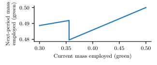
(b) Employment of Greens

Figure 1: Referrals for a group happen according to a Poisson distribution: $\hat{P}(k|m)=\frac{m^{k}e^{-m}}{k!}$; and parameters values are: $n_{b}=n_{g}=.7$ so that $n=1.4$; and $v_{i}$ takes on three values $0,\frac{1}{3}$, and $1$, with equal probability. We plot the mass of blue and green workers hired on the referral market, and the next-period employment mass of green workers, as a function of the current employment rate of green workers.

Figure 1 shows an example of this phenomenon in which referrals are made uniformly at random among a group. Increasing the current mass of employed green workers towards the unbiased employment rate of $1/2$ increases the number of referrals green workers get. The direct effect is then seen via the increase in green workers hired on the referral market. However, additionally the overall probability of not getting a referral decreases, which leads to more lemons in the pool, and so the hiring threshold on the referral market drops. In particular, at a current employment of greens below $\approx 0.355$, the threshold is such that referred workers with the middle value of $\frac{1}{3}$ are not hired whereas they are once green employment rises above $\approx 0.355$ (see Panel 1(a)). This change in the equilibrium threshold is the indirect effect: referred workers with the middle productivity value are hired for the higher current employment of green workers; but this disproportionately helps blue workers as they have more referrals. As a result, the next-period employment rate of green workers is lower when their current employment rate is just above $\approx 0.355$ rather than just below $\approx 0.355$ (see Panel 1(b)).

3.4 Dynamics and Immobility Across Periods

We now examine the long-run dynamics of the employment levels of the groups.

In this subsection, we presume that the minimum wage is low enough so that firms find it worthwhile to hire from the pool in steady state. Without this condition, it is possible to get cycles in whether firms hire from the pool which can preclude convergence.

If one group is more self-biased in giving referrals than the other group, then that group gets relatively more referrals, and they will dominate employment in the long-run. Convergence to balanced employment thus requires a balance in referral rates (recall the definitions in Section 3.2).

Proposition 2.

There exists a unique steady-state employment rate for each group. The steady-state employment rates are balanced ($\frac{e_{b}}{e_{g}}=\frac{n_{b}}{n_{g}}$) if and only if there is referral balance ($\frac{R_{b}}{R_{g}}=\frac{n_{b}}{n_{g}}$). If there is referral balance, then convergence to the steady state occurs from any starting employment levels.

Existence of a steady state follows from a standard fixed-point argument. Uniqueness is more subtle, and depends on bounding the slope of how next-period employment of a group can grow as a function of increasing current employment of that group. If that “slope” is everywhere less than one, then there can be only one fixed point. The idea is as follows. Adding one extra green today leads to at most one more green referral, and possibly a blue referral or a blue hire. So, the direct effect is at most one. When greens are in the minority, raising green employment increases the number of referrals and makes the lemons effect worse. This lowers the threshold and leads to relatively more blue hires, again working against green hires. Once greens are in the relative referral majority, then further increasing their numbers decreases the overall number of referrals and so actually decreases the lemons effect and raises the threshold – now disadvantaging the greens again since now they are getting more referrals. This establishes the uniqueness. Employment rates equal to population shares is a fixed point if referrals are balanced and not otherwise, and so uniqueness implies that this is the steady state if (and only if) balance holds. Convergence is again more subtle. Balanced referrals can be shown to imply a monotonicity, so that a group that is underemployed gains employment but never more than to a balanced level. However, without referral balance, the indirect effect can dominate and lead to a situation where the change in employment overshoots the steady-state.

Proposition 2 shows that if referrals are balanced, then initial employment rates become irrelevant in the very long run. Of course, that is over generations, and so with high rates of homophily, inequality could persist for many generations.

3.5 Productivity with Unequal Referrals

We define productivity to be the total value of employed workers, plus the outside option ($w_{min}$) for all the unemployed workers.

Equilibria have inefficiencies: firms hire referred workers with productivity below other workers in the pool. Nonetheless, one can show that an equilibrium is still constrained efficient – the threshold for hiring referred workers that maximizes total production is the unique equilibrium threshold. A formal statement of this together with a proof is given in Appendix B.3.

However, although each equilibrium uses the best threshold it can, the equilibrium varies with the how unequal referrals are distributed across groups. More equal initial employment results in more equally spread referrals and increases productivity.

To understand how productivity changes with how unequal referrals are distributed across groups, it is useful to note that a single referral is productivity enhancing: If a worker has high productivity (above the equilibrium threshold), then that worker is hired. If the referred worker has low productivity, then the firm has the option of taking a match from the pool. When some worker gets two or more referrals instead of one, then that does not improve the matching of that worker beyond the first referral – if they are low value then the referrals are all wasted, and if they are of high value then any referral past the first one is wasted. This then suggests that any change that increases the probability of not getting a referral, $P(0)$, is detrimental to productivity – the total value of production in the society goes down as fewer high-value workers are hired overall in the economy.

There are some subtleties – unequal referrals across groups, and hence a higher aggregate probability of not getting a referral, implies that that there are fewer lemons in the pool, making the pool more productive and raising the equilibrium threshold. The proof shows that this countervailing force is always overcome. The basic intuition is that having a higher probability of not getting a referral means that fewer workers get vetted overall, and more ultimately end up being hired without any vetting (lemons or otherwise). Ultimately, jobs that are not filled by a high-value worker end up being filled by someone of lower value or not filled at all (depending on the equilibrium, presuming that we are not changing from one type of equilibrium which hires from the pool to the other which does not), and replacing those with high value is good. The full proof takes care of all the possible cases, including in which we change whether workers are hired from the pool or not.

Proposition 3.

Suppose that referrals are purely homophilous; i.e., $h_{b}=h_{g}=1$. Employment ratios that are closer to being population-balanced strictly increase productivity: that is, if $\frac{e_{b}^{\prime}}{e_{g}^{\prime}}>\frac{e_{b}}{e_{g}}\geq\frac{n_{b}}{n_{g}}$, then the next-period productivity in the equilibrium with current employment $(e_{b}^{\prime},e_{g}^{\prime})$ is strictly less than the next-period equilibrium productivity with current employment $(e_{b},e_{g})$.

The proof of Proposition 3 appears in Section B.1 of the supplemental appendix.

This indicates that although an equilibrium is constrained efficient in terms of firms’ hiring decisions given a certain mix of referrals, if that mix of referrals can be made more balanced, that would improve overall productivity. We examine such policy interventions in Section 4.

3.6 Costly Investment and Immobility

There are (at least) two ways in which inequality may persist indefinitely. One is, as outlined in the proposition, that there is an imbalance in referral rates – for instance with one group being more homophilous in its referrals than another. A second is that there may be additional incentives in the matching process that induce long-run inequality in employment rates. For instance, if workers must make a costly investment – e.g., in education – to realize a productive value, then we may observe perpetual immobility and inequality. In particular, since Proposition 1 implies that the expected wage of blue workers of participating in the labor market is greater than that of green workers, if there is some cost to educating one’s self before knowing whether one will have a referral, then for some investment costs green workers will not invest while blue workers will.

Since poverty traps are analyzed elsewhere, we do not elaborate further here, but we note that this model induces a robust poverty trap if workers have to invest in order to be productive.

4 Affirmative Action and Other Policies

A government can impose policies to alleviate the inequality and immobility that arise in referral networks. Moreover, as we have seen above, this not only improves ‘fairness,’ but can also increase overall productivity. We now analyze some prominent policies in the context of the blue-green setting described above.

For simplicity, throughout this section, we specialize to the situation in which blues and greens are both completely homophilous, so that $h_{b}=h_{g}=1$. Furthermore, we presume that firms hire when indifferent ($r=1$). These restrictions simplify the exposition, but are not necessary for the results that follow.

Without loss of generality, suppose that blues are relatively advantaged in starting employment, so that $\frac{e_{b}}{e_{g}}>\frac{n_{b}}{n_{g}}$.

4.1 Affirmative Action’s Dynamic Impact

Affirmative action policies change hiring thresholds with the intent of moving the employment distribution to be closer to balanced. This not only has immediate effects, but can also have longer term effects since referrals are also moved closer to being balanced. This points out an interesting aspect of affirmative action: it not only increases short-term equality of employment based on characteristics, but it also has long-term network effects that further reduce inequality and improve mobility and future productivity.

The complication, as we have seen above, is that a change in employment rates can also impact the equilibrium referral hiring threshold, which can result in an indirect effect that can be countervailing. In spite of that effect, there is much that we can deduce about the impact of such policies.

First, we show that (generically) a small one-period increase in the employment of the under-employed group increases their employment as well as overall production in all subsequent periods.

Proposition 4.

Let $F$ be any discrete distribution. For almost every $e_{g}$, there exists $\varepsilon>0$ so that an increase in $e_{g}$ by up to $\varepsilon$ leads to a strict increase in total production as well as green employment in all future periods (relative to what they would have been without the increase).

Thus, affirmative action has long-run implications and even a one-time policy can have long lasting positive effects on both equality and total production.

We illustrate these dynamic effects in Figure 37, which pictures the impact of a one time increase in the employment of greens. Referrals are again made uniform at random among a group. We see three long-term effects. First, increasing current employment of greens increases their employment in all periods relative to what it would have been without. Second, the difference in average wages between blues and greens is decreased in all periods. Third, this also improves production in all subsequent periods, but has a cost in the current period from replacing referred blues with draws from the pool to get sufficient greens.

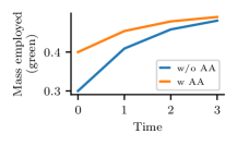
(a)

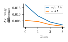
(b)

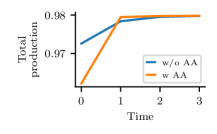
(c)

Figure 2: Referrals for a group happen according to a Poisson distribution: $\hat{P}(k|m)=\frac{m^{k}e^{-m}}{k!}$; and parameter values are: $n_{b}=n_{g}=1$ so that $n=2$; and $v_{i}$ takes on two values $0$ and $1$, with .95 and .05 probability, respectively. The blue line is without affirmative action and orange is with affirmative action in the first period. The graphs above show the dynamic effects of changing green employment in from .3 to .4 by randomly choosing some firms with high value referred blues and having those firms to go to the pool.

The above example works cleanly since it only involves two productivity levels. With more productivity levels, large changes in employment can lead to threshold reversals and so large affirmative action policies can involve some non-monotonicites in some future periods. In particular, as shown in Section 3.3, an increase in the current employment of a disadvantaged group does not necessarily increase their next-period employment rate compared to what it would have been, due to the indirect effect operating through the hiring threshold. As a result, employment rates in some future period can, under some particular situations, be further apart than they would have been without an affirmative action policy (furthermore implying a decrease in total production in that period relative to that without the policy). As shown in Proposition 2, there would still be eventual convergence, given referral balance, but it could be sped up in some periods and slowed down in others. Thus, care is warranted in designing such policies given the potential indirect effects due to changes in equilibrium lemons effects.

The long-term impact of affirmative action policies from a one-time intervention is important in light of the issues raised by Coate and Loury (1993). They show that a long-term affirmative action policy can make a group dependent upon the policy and reduce their skill acquisition. Our results showing that a one-time intervention can have a lasting impact implies that such policies can be designed to be temporary, thus avoiding the Coate and Loury (1993) conundrum.

4.2 Optimizing Affirmative Action

Next, we examine which of the two basic approaches to affirmative action – encouraging the hiring of greens versus discouraging the hiring of blues – is more effective.

More specifically, one can increase green employment by either encouraging the hiring of more greens from referrals (which decreases the number of blues hired from the pool), or discouraging the hiring of blues from referrals (and thus hiring relatively more greens from the pool). One can enact these by, for instance, paying a small subsidy for each green worker who is hired or else taxing firms that hire a blue worker. One can also think of a broader class of interventions that include quotas and caps for hires on the referral market. To capture the tradeoff between promoting green workers and demoting blue workers, we compare the effects of increasing the mass of green workers versus decreasing the mass of blue workers hired on the referral market.

Both types of policies distort the optimal hiring decision so that total production decreases in the period where the affirmative action is put in place, but have the longer term impact of increasing productivity in future periods. In general, one of the two policies will dominate the other, in the sense that it achieves the same desired goal at a lower reduction in current production.

We illustrate this trade-off in the simple case in which workers are either of high or low value, $v_{H}$ or $v_{L}$. Let $\tilde{v}$ be the expected value in the pool and $f_{g}$ the fraction of workers in the pool that are green, both in the absence of any intervention. Without any intervention, high-valued referrals are hired, and otherwise the firm hires from the pool. Consider a small intervention – just changing a few hires so that we don’t effect the pool value substantially. If one increases the number of green referrals hired, then that puts in a low valued worker in place of a random draw from the pool, so the lost productivity is $\tilde{v}-v_{L}$ and the gain in green employment is $1-f_{g}$. If one decreases the number of blue referrals hired, then that puts in a random draw from the pool in place of a high valued worker, so the lost productivity is $v_{H}-\tilde{v}$ and the gain in green employment is $f_{g}$. Which of these is better depends on whether the value of the pool is closer to the high value or the low value as well as the fraction fraction of workers in the pool that are green.

Proposition 5.

One prefers to increase green employment by some $\varepsilon$ close to 0 by increasing green referral hires if and only if

$$\frac{1-f_{g}}{\tilde{v}-v_{L}}>\frac{f_{g}}{v_{H}-\tilde{v}}.$$

Furthermore, as long as both policies can achieve the desired employment bias, using one of them as opposed to a combination of them is optimal.

The proof of Proposition 5 appears in Section B.1 of the supplemental appendix.

In addition to the type of affirmative action policy, effectively decreasing the number of blue or increasing the number of green referrals hired, one can also optimize over the size of the policy, i.e., how many hiring decisions should be changed. As one increases the size of the affirmative action policy, two things change: 1) the composition of the pool; and 2) the composition of the referral market (both due to not hired blue or hired green referral workers).

The first is important as those are the workers with which, for example, high-value blue referral workers are replaced with: a firm does not hire their high-value blue referral worker and instead hires from the pool. The second change matters, as those are the ones potentially forced to be hired or not. Interestingly, as in Proposition 5, changes in the composition of the pool may not affect the cost-benefit analysis of an affirmative action. Such changes simply reflect the possibility of undoing some of the policy, e.g., hiring a high-value blue referral worker from the pool who was forced to enter the pool. As Proposition 5 only deals with a two-type value distribution, the composition of workers on the referral market does not matter as long as there are e.g., low-value green workers.

However, this is not true more generally. When forcing firms to hire green referral workers that otherwise would not have been hired, the optimal policy ensures hiring of such green workers with the highest values. This value is decreasing the more green referral workers are hired so that the productivity decrease of hiring such workers becomes larger.

4.3 Forward-Looking Firms

Our analysis has examined myopic firms. For most of our analysis myopic and forward-looking firms would act similarly, since the value of the future referrals only differ across workers once we get to our green-blue analysis. When greens are relatively under-employed, hiring a green worker is more valuable than hiring a blue worker for two reasons. First, green workers in the pool suffer from less of a lemons effect and so are more productive on average compared to blue workers in the pool. Second, greens are more likely to refer other greens and those referred greens are less likely to have multiple referrals than a referred blue. So, a firm expects to hire referred greens at lower wages than referred blues. This provides a natural form of affirmative action: firms can have a preference for hiring the relatively disadvantaged group compared to the advantaged group, both at the referral stage and the pool stage.

If the green/blue distinction can be observed by firms, then that may cause them to (slightly) prefer to hire greens. To illustrate this effect, we revisit the example from Figure 37, but instead of affirmative action, we consider what happens if firms can see whether a worker is blue or green, and can repeatedly search in the pool by paying a search cost each time. Firms’ costs of repeated search are distributed uniformly on [0,1]. For simplicity, firms only consider the higher expected productivity of green workers in the pool rather then the network effects.

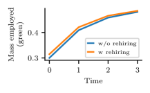
(a)

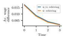
(b)

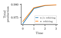
(c)

Figure 3: The blue line is with myopic firms. The orange line is when firms can redraw from the pool. The parameters are as in Figure 37, with costs of redrawing from the pool uniformly distributed on [0,1].

Without being able to distinguish blues and greens, the firms would never pay additional costs for more draws from the applicant pool; but if they can distinguish greens from blues, then for small enough costs they prefer to keep searching for a green. This means that more greens get hired from the pool. The effects of this policy are pictured in Figure 3. We see that employment and wages both increase for greens in all periods, as does overall productivity. This has similar directional effects as affirmative action, except that productivity increases in all periods rather than only in the future.

4.4 Firing Workers and Inequality

Referrals allow firms to learn about the type of a worker and are thus valuable to firms as well as the workers who are referred. Beyond affirmative action, there are other policies affecting what firms learn about workers that can also reduce inequality. In this section, we consider how the market changes when firms can fire a worker and replace them with another worker from an open application.

In particular, let us suppose that after some time has elapsed, firms have learned the value of any worker they have hired (they already know the value of a referred worker if they kept her, so this applies mainly to a worker hired from the pool), and can then choose whether to fire that worker and hire a new one from the pool for the remaining time. This makes hiring from the pool more attractive, as there is less expected loss if the worker turns out to have low productivity.

Let $\lambda$ be the fraction of time that is left in the period for which they would get the replacement worker, and $1-\lambda$ be the fraction of the period that has to elapse before a firm can fire a worker. In equilibrium, as we prove below, a firm would never fire a referred worker that they kept initially, so the decision will only be relevant for workers they hired from the initial pool.

The timing is as follows:

1. Firms get referrals from their current employees.

2. Firms can choose whether to (try to) hire a referred worker and make an offer.

3. Referred workers with offers can choose to accept any of those offers (in which case they exit with the firm) or to go to the pool, all other workers go to the pool.

4. Firms that did not hire a referred worker can choose whether to hire from the pool.

5. After $1-\lambda$ of the period has elapsed, firms can choose to fire their current worker.

6. All fired workers return to the pool, joining all other workers who are not employed.

7. Firms that have fired a worker can choose to hire from the new pool.

We refer to these pools as pool 1 and pool 2, respectively. We assume that the distribution of values is high enough so that firms prefer to hire from these pools than to have no worker at all in order to simplify the exposition; the full details are worked out in the appendix.

A firm’s production is given by $1-\lambda$ of the value of its worker before any firing, and then $\lambda$ of its worker that it has after any firing and rehiring decisions are made. An equilibrium is now characterized by a pair of threshold strategies: referred workers are hired if their value is above $\tilde{v}_{1}$ and otherwise firms hire from the first pool. Then at the second decision point firms fire workers, when given the opportunity, if the worker’s value is below $\tilde{v}_{2}$. Again, firms can mix with some probability when indifferent.

Let ${\mathrm{E}}_{\tilde{v}_{1},r_{1}}[v_{i}|i\in\text{pool }1]$ be defined as in equation (1) and ${\mathrm{E}}_{\tilde{v}_{1},\tilde{v}_{2},r_{1},r_{2}}[v_{i}|i\in\text{pool }2]$ denote the expected value in pool 2 if the hiring threshold on the referral market is given by $\tilde{v}_{1}$, the firing threshold by $\tilde{v}_{2}$, firms hire referral workers at the margin with mixing parameter $r_{1}$ and firms fire workers at the margin with mixing parameter $1-r_{2}$. The threshold strategies then imply the following two equilibrium conditions:

$$\tilde{v}_{1} =(1-\lambda){\mathrm{E}}_{\tilde{v}_{1},r_{1}}[v_{i}|i\in\text{pool }1]+\lambda{\mathrm{E}}_{\tilde{v}_{1},r_{1}}[\max\{v_{i},\tilde{v}_{2}\}|i\in\text{pool }1];$$ (4)

$$\tilde{v}_{2} ={\mathrm{E}}_{\tilde{v}_{1},\tilde{v}_{2},r_{1},r_{2}}[v_{i}|i\in\text{pool }2].$$ (5)

Let $\tilde{v}$ denote the hiring threshold for the model without firing (so that $\lambda=0$). For $\lambda\in(0,1]$, not hiring a referred worker and instead going to pool 1, now features an option value: the firm randomly draws a worker but may get a second draw to replace the worker if the worker’s value is too low; a draw from pool 2. As a result, firms have a higher threshold on the referral market compared to the base model. This lessens the lemons effect in the first pool and so the first pool value is actually higher than $\tilde{v}$. The second pool, however, has a worse lemons effect since it then includes all fired workers as well as rejected referral workers. The fact that the second threshold is less than $\tilde{v}$ takes some proof, but is true. Essentially, the extra opportunity to fire improves the overall productivity, and so the workers left in the second period pool are worse than in the case where there is just one chance to hire.

Lemma 3.

There are unique thresholds $(\tilde{v}_{1},\tilde{v}_{2})$ and mixing parameters $(r_{1},r_{2})$ with $r_{2}$ arbitrary satisfying equations (4) and (5). For $\lambda>0$, they satisfy $\tilde{v}_{2}<\tilde{v}<\tilde{v}_{1}.$

Note that our base model is nested in this formulation with $\lambda=0$.

The equilibrium thresholds, as before, are unique, so that we can perform comparative statics with respect to unique equilibrium quantities. Firms have a higher hiring threshold on the referral market when $\lambda>0$ and rely more on search via open applications. The additional weight on open applications in the hiring process increases the opportunities for disadvantaged groups – e.g., the green workers – and improves their employment prospects. The willingness of firms to engage in further search decreases the production in the first part of the period.

However, as the proposition below shows, overall production – the weighted production in the two parts of the period – increases with $\lambda$. Thus, efficiency and equality are always greater when there are opportunities for firms to fire their worker.

Proposition 6.

For any $\lambda>0$, the employment rate bias is less than, and total production is greater than, what it would have been without the opportunity to fire ($\lambda=0$). In terms of timing within the period: (i) both the employment bias in favor of blue workers and productivity measured before the firing stage are decreasing in $\lambda$; and (ii) the productivity at the end of the period is increasing in $\lambda$ while the employment bias in favor of blue workers at the end of the period changes ambiguously.

The proof of Proposition 6 appears in Section B.1 of the supplemental appendix.

Comparing productivity and equality between two different positive values of $\lambda$ is nuanced. While efficiency unambiguously increases the greater the opportunities for firms to fire a worker, the employment rate bias at the end of the period may behave nonmonotonically in $\lambda$. More use of the first pool leads to a worse lemons effect in the second pool, which can disadvantage the greens. As a result, the overall implication for the employment rate bias measured at the end of the period is ambiguous.

5 The Impact of Changes in the Referral Distribution on Inequality and Productivity

In the previous sections we identified relationships between immobility, inequality, and productivity; and also found that they changed as referrals were rearranged - for instance spread more evenly between greens and blues. These sorts of changes in the distribution of referrals spread referrals among fewer people. In this section, we examine some subtleties. Although we documented that having referrals more concentrated among one group leads to differences between groups, that does not indicate whether it leads to an overall increase in inequality when measured across the society as a whole, for instance, via a Gini coefficient. It turns out that the changes in referrals that impact productivity are actually different from those that impact overall inequality, and overall inequality depends on some specifics of the distribution of values.

Let $P(2+)=\sum_{k\geq 2}P(k)$ denote the fraction of workers (of any type) who get two or more referrals. $P(0)$ and $P(2+)$ can be thought of as two ways of changing referral inequality: increasing the probability of not getting a referral (increasing $P(0)$); and increasing the probability of getting multiple referrals (increasing $P(2+)$). As we will see, changes in $P(0)$ impact economic productivity whereas income inequality, as captured by the Gini coefficient, is also impacted by $P(2+)$.

Neither of these implies the other. It is possible to have $P^{\prime}$ increase the probability of not getting a referral but decrease the probability of getting multiple referrals compared to $P$, or vice versa. However, as we show in Section 5.3, $P(0)$ and $P(2+)$ can be closely tied together under natural assumptions, implying improvements in productivity and inequality go hand-in-hand in these economies.

5.1 Concentrating Referrals Decreases Productivity

In this subsection, we presume that firms hire when indifferent ($r=1$). The mixing cases do not change any of the productivity results, but comparing across distributions requires specifying the mixing for each distribution, which has no real consequence but complicates the proofs. We first investigate how equilibrium productivity changes with the underlying distribution of referrals. Section 3.5 and Proposition 3 established that productivity increases if employment ratios across groups are closer to being population-balanced. Here, we generalize the result and state it with respect to the aggregate probability of not getting a referral.

Proposition 7.

Consider two referral distributions, $P$ and $P^{\prime}$, and corresponding unique equilibria ${\tilde{v}}$ and ${\tilde{v}}^{\prime}$, respectively. If $P^{\prime}$ increases the probability of not getting a referral compared to $P$ (i.e., $P^{\prime}(0)\geq P(0)$), then

• ${\mathrm{E}}_{\tilde{v}^{\prime}}[v_{i}|i\in{\mathrm{pool}}]\geq{\mathrm{E}}_{\tilde{v}}[v_{i}|i\in{\mathrm{pool}}]$, and so there is a weak decrease in the lemons effect and a weak increase in the expected value of workers in the pool;

• and the total production in the economy associated with $P^{\prime}$ is less than or equal to that associated with $P$.

All comparisons are strict if there is a strict increase in the probability of not getting a referral (i.e., $P^{\prime}(0)>P(0)$).

Proposition 7 states that concentrating referrals among a smaller part of the population, leads to a decreased lemons effect and decreased productivity. Increasing the probability of not getting a referral reduces the lemons effect since fewer people are rejected and pushed into the pool (even accounting for the raised threshold, as that raised threshold is itself a reflection of the extent of the lemons effect). In fact, the lemons effect moves exactly with the total production in the economy: the average productivity of the workers in the pool equals the average productivity of the unemployed, and thus counter-weights the average productivity of the employed. Intuitively, production worsens since fewer workers are vetted, and less information leads to worse matching.

A change in the referral distribution can be the result of a change in macroeconomic conditions. For example, if fewer firms are hiring, then fewer people get referrals, but total employment is also changed. We study how such changes affect inequality and inefficiency in Section 5.4.

5.2 The Impact of Concentrating Referrals on Wage Inequality

In Section 3.2, we studied how employment bias via unequal referrals leads to inequality across groups (Proposition 1). However, this analysis does not speak to aggregate measures of inequality in society as a whole and how they respond to changes in the referral distribution. This is the subject of this section: the impact on wage inequality, which in this model is equivalent to income inequality (more comments on this below) from changes in the referral distribution.

The first thing to note is the key factor in determining the wage distribution in our model is the number of people who get more than one referral: those are the people who have some competition for their services and earn above the minimum wage. Thus, rather than how many people get referrals, what is key here is what fraction of people get multiple referrals. The probability of not getting a referral still determines the expected value from hiring from the pool, and thus impacts wages that people with multiple referrals obtain, so it is also involved but with a different (marginal) effect.

To measure inequality, we use the Gini coefficient of wages (see Equation 6 for a formal definition in our setting). As comparing distributions is generally an incomplete exercise, using such a coefficient allows one to make comparisons of partially ordered distributions. However, even using this standard one-dimensional measure, and looking at simple settings, we will see that inequality can move in different ways from the same comparative statics, depending on the specifics of the environment.

One might expect that an increase in the probability of getting multiple referrals would be sufficient to increase inequality, but things are not so direct. First, even if few workers are high-wage earners, increasing the size of that group can actually increase or decrease inequality, depending on relative wages and the relative size of the group to begin with, as the Gini coefficient makes relative comparisons. In addition, increasing the probability of getting multiple referrals can alleviate the lemons effect if accompanied by a decrease in the probability of not getting a referral. This tends to decrease the wages of the workers who have multiple referrals, lowering the high wage, which can then decrease inequality. Thus, there can be different sorts of countervailing effects.

To get a characterization of when inequality is raised by increasing the probability of getting multiple referrals, for this subsection only, we consider a situation in which productivity takes on two values $v_{H}>v_{L}$, with fraction $f_{H}$ of the population being of the higher productivity. As the minimum wage equals the value of workers’ outside options, this implies that there are just two levels of wages. All of the countervailing effects described above already exist with just two types, and this simplification makes it easier to see the intuition.

Let $\pi_{H}=P(2+)f_{H}$ denote the fraction of workers who earn the high wage, $w_{H}=v_{H}-\tilde{v}+w_{min}$ denote the equilibrium wage of a worker with high value, and $\pi_{L}=(1-P(2+)f_{H})$ be the remaining fraction of workers, who all earn the minimum wage. Let $W_{L}=\frac{w_{min}}{w_{H}}$ denote the low wage relative to the high wage. One can write the Gini coefficient, denoted by $Gini$, of an economy as follows:

$$Gini=\frac{\pi_{H}\pi_{L}(w_{H}-w_{min})}{\pi_{H}w_{H}+\pi_{L}w_{min}}=\frac{\pi_{H}\pi_{L}(1-W_{L})}{\pi_{H}+\pi_{L}W_{L}}=\frac{\pi_{H}(1-\pi_{H})(1-W_{L})}{\pi_{H}+(1-\pi_{H})W_{L}}.$$ (6)

Let us consider what happens when the fraction of people earning the high wage is increased ($\pi_{H}$ is increased), which is a consequence of increasing the probability of getting multiple referrals. Straightforward calculations show that:

$$\frac{\partial Gini}{\partial\pi_{H}}=\frac{(1-W_{L})(W_{L}\pi_{L}^{2}-\pi_{H}^{2})-\frac{\partial W_{L}}{\partial\pi_{H}}\pi_{H}\pi_{L}}{(\pi_{H}+\pi_{L}W_{L})^{2}}.$$

The change in the Gini coefficient consists of two parts: the effect of changing the fraction of people earning the high wage, and then the effect of changing the wage via the lemons effect.

The first part (ignoring the term including $\frac{\partial W_{L}}{\partial\pi_{H}}$) is positive for low $\pi_{H}$ and high $W_{L}$, but then becomes negative as $\pi_{H}$ increases and $W_{L}$ decreases. However, then the overall expression is impacted by the $\frac{\partial W_{L}}{\partial\pi_{H}}$ term, which accounts for the lemons effect. The change in the lemons effect depends on both the probability of not getting a referral as well as multiple referrals.

To fully sign the $\frac{\partial W_{L}}{\partial\pi_{H}}$ term, we also need to know what happens to the probability of not getting a referral. In particular, the change in $W_{L}$ comes from the change in $w_{H}$, which is exactly governed by the probability of not getting a referral. Knowing how $P(2+)$ changes, tells us about $\pi_{H}$, but we need to know how $P(0)$ changes to determine the change in $w_{H}$. If the change in the referral distribution is comprised of both an increase in the probability of not getting a referral and the probability of getting multiple referrals, then the increase in $\pi_{H}$ is accompanied by an increase in $P(0)$ which, using Proposition 7, decreases the lemons effect and thus the high wage so that $\frac{\partial W_{L}}{\partial\pi_{H}}>0$. This then counteracts the impact of the first term for low $\pi_{H}$ and can reverse the change in the Gini coefficient.

These results are summarized in the following proposition, which should be clear from the above discussion, so we omit a formal proof. Let $I_{H}=\pi_{H}w_{H}$ and $I_{L}=\pi_{L}w_{L}$ denote the total income going to the high and low wage earners, respectively.

Proposition 8.

The Gini coefficient decreases with an increase in the probability of not getting a referral (an increase in $P(0)$), holding $P(2+)$ constant. And, holding $P(0)$ constant, the Gini coefficient increases with an increase in the probability of getting multiple referrals (an increase in $P(2+)$) if and only if $I_{L}\pi_{L}>I_{H}\pi_{H}$.

The comparison $I_{L}\pi_{L}>I_{H}\pi_{H}$ captures the relative total wages, population weighted, which is important in determining whether the inequality is due to most of the society’s income coming from the low wage, which holds for low values of $\pi_{H}$ and ${w_{H}}$, or the reverse, which determines whether things are getting more or less equal.

Proposition 8 implies that a mean-preserving spread in $P$, such that the probability of not getting a referral goes down and the probability of getting multiple referrals goes up (presuming $I_{L}\pi_{L}>I_{H}\pi_{H}$), pushes up the fraction of high wage earners and also increases their wage due to an increased lemons effect, thus increasing the Gini. If instead (again presuming that $I_{L}\pi_{L}>I_{H}\pi_{H}$), we consider a first-order dominance shift in $P$, then there are countervailing forces: more people earn the higher wage, but that wage goes down due to an improved value of the pool. Either force can dominate depending on the particular parameters.

In Section B.4 of the supplemental appendix, we discuss what happens when firms’ profits are also included in the calculations of inequality.

5.3 Referrals Tie Immobility, Inequality and Inefficiency together

Even though changes in the probability of not getting a referral and getting multiple referrals are logically distinct, many of the interesting comparisons are ones in which they happen together. This can be caused by a variety of factors.

In Section 3.1, we have shown that if people belong to groups (e.g., ethnic or geographic), one group has an advantage in terms of its initial employment, and people tend to refer people of their own group, then this leads to an aggregate referral distribution with a higher probability of not getting a referral. This was driven by the assumption that the probability of not getting a referral for a group is strictly convex in the average number of referrals the group gets. Here, we show that unequal employment across groups can similarly lead to an aggregate referral distribution with a higher probability of getting multiple referrals. This holds when the probability of getting multiple referrals for a group is also strictly convex. For a fixed but arbitrary process (e.g., uniform at random), the second derivative of this probability depends on the probability of getting exactly one referral in that group. Thus, for low levels of referrals, strict convexity of the probability of getting multiple referrals for a group follows.

For simplicity, in addition to the same setting as in Section 3.1, assume that referral-bias parameters satisfy $h_{b}>1-h_{g}$. Let $\overline{e}_{b},\overline{e}_{g}$ be the unique employment rates that equate the average number of referrals across groups, $m_{b}=m_{g}$.

Lemma 4.

Suppose that $\hat{P}(0|m)$ is strictly convex in $m$; and $\hat{P}(2+|m)$ is strictly convex in $m$ for feasible average numbers of referrals $m$. Then:

• the aggregate probability of not getting a referral, $P(0|m_{b},m_{g})$, and the aggregate probability of getting multiple referrals, $P(2+|m_{b},m_{g})$, are strictly convex in employment levels; and

• both $P(0|m_{b},m_{g})$ and $P(2+|m_{b},m_{g})$ are minimized at $\overline{e}_{b},\overline{e}_{g}$.

Lemma 4 ties together immobility, inequality and inefficiency through the referral distribution. For example, if referrals are purely homophilous, $h_{b}=h_{g}=1$, and the assumptions in Lemma 4 hold, then a employment ratios that are closer to being population-balanced have the following effects:

• Immobility: employment is closer to being population-balanced in every future period (for discrete $F$ and small changes in initial employment; Proposition 4).

• Inequality in Wages: future Gini coefficients decrease under the conditions stated in Proposition 8.

• Inefficiency: future productivity increases (Proposition 3).

Hence, if people belong to groups (e.g., ethnic or geographic), one group has an advantage in terms of its initial employment, and people tend to refer people of their own group, then this can lead to referrals with a higher probability of not getting a referral and multiple referrals compared to a world that is group-blind (e.g., see Zeltzer (2020) for evidence of exactly this effect in the context of gender homophily in referring physicians).

In addition to differences in employment (with similar referral-bias parameters), it could also be that some groups get relatively more referrals per capita due to biases in referrals, $\frac{R_{b}}{R_{g}}>\frac{n_{b}}{n_{g}}$ (e.g., in some settings males are more strongly biased towards referring males than females are to referring females, as seen in Lalanne and Seabright (2016)). A variant of Lemma 4 – with no employment bias and varying the extent of the referral bias – implies that, under some conditions, a large referral bias (e.g., favoring men) increases the aggregate probability of not getting a referral and getting multiple referrals.

Lastly, the probabilities of not getting a referral and getting multiple referrals may also be tied together if people become more likely to refer more-popular friends than a friend at random, since their more-popular friend might be in a better position to return the favor some day. This causes an increase in $P(0)$ as well as $P(2+)$.

5.4 The Impact of Macroeconomic Conditions on Productivity and Inequality

As a last comparative static, we examine how macroeconomic conditions, such as the number of jobs available, affect productivity and inequality among those being hired in any given period. To answer this, we hold the network of connections fixed, but randomly remove some firms from the job market. In particular, if a mass $\kappa<1$ of firms are no longer hiring, what is the impact on the job market? Of course, this decreases overall employment. The more subtle question is what happens to the average productivity per employed worker and to the inequality in the society.

First, let us consider the productivity per employed worker. The drop in firms decreases the mass of workers who are looked at on the referral market, $(1-P(0))n$, by some positive amount (at most $\kappa$). As a result, the lemons effect decreases and the remaining firms now have better outside options and their production, so productivity per worker, increases.

Second, firms that do remain are less likely to face competition from other firms for their referred workers. This leads to a decrease in average wages because of the reduced competition and also the lower lemons effect and improved alternative of hiring from the pool.

These results are summarized in the following proposition, in which we presume that firms would hire from the pool if $\kappa=0$.

Proposition 9.

Suppose a mass $\kappa<1$ of firms no longer hire on the job market. Then:

• total production decreases;

• production per employed worker increases; and

• the old wage distribution of wages first-order stochastically dominates the new one.

All comparisons are strict if $\kappa>0$.

The consequences for inequality measured by the Gini coefficient are complicated as the Gini coefficient itself is nuanced (see Section 5.2). A downturn in the aggregate economy (some firms are removed from the job market) results in both an increase in the probability of not getting a referral, $P(0)$, as well as a decrease in the probability of getting multiple referrals, $P(2+)$. Thus Proposition 8 suggests that the Gini coefficient tends to decrease in economic downturns (under some conditions).

Are different groups (Section 3.1) differentially affected by such downturns? There are two effects. One is the reduction in the lemons effect: this unambiguously reduces inequality across groups as it disproportionately lowers the advantage of referrals both in terms of wages and the chances of being employed. The second effect is that workers lose referrals, which actually relatively hurts the disadvantaged group more, since more of them who are getting referrals are only getting one referral and lose that referral. In particular, if $\hat{P}(0|m)$ is convex in $m$ (as is naturally the case for most distributions, as discussed above), then for purely homophilous groups, the disadvantaged group, rather than the advantaged group, loses a larger fraction of workers looked at on the referral market.

6 Concluding Discussion

We have shown how referrals can lead to inequality, inefficient production, and persistent differences across groups. We have also shown that there is a relationship between immobility, inequality, and inefficiency: concentrating referrals among one group decreases productivity and mobility, and increases inequality. However, we have also showed that the relationships between these are more subtle that one might superficially imagine, due to the lemons effect.

As we have seen, immobility, inequality, and inefficiency can be counteracted by policies – for instance, affirmative action policies – that encourage hiring from the pool. These policies have long-run impacts even if enacted for short periods. We focused on whether the policy penalized the hiring of blues, or enhanced the hiring of greens; but there are many ways in which this can be done. For instance, requiring interviewing of qualified minorities for open positions as in many sports leagues for coaching positions, is a way to force firms to investigate workers from the pool. There are also other policies that have similar effects, for instance simply subsidizing internships of workers from the pool, or providing more information about non-referred workers, via various sorts of certification. In addition, even though full efficiency is not reached in the setting with firing, the ability to fire does improve overall productivity and reduce inequality; which provides insight into one advantage of flexible labor markets.

The model that we have presented here should be useful as a base for additional explorations. For instance, we have not modeled how firms choose how many people to hire. Firms’ decisions on hiring could react to the attractiveness of the pool and how much access they have to referrals, and so wider-spread referrals could also lead to the creation of new openings, amplifying some of the effects we have shown. Another effect of referrals is on how long workers last at their current jobs, and allowing for reduced turnover due to referrals would also be interesting to explore, but would require changes to the model. One could also explore career choices using this model as a base. People would (inefficiently) be driven to choose professions of their family and friends, even if they might be more talented in another profession, because of the improved wage and employment prospects due to referral connections. Finally, firms sometimes hire referred workers as favors to their current employees (or because the current employee lied), even when the referred workers are of low value. Such effects could exacerbate the advantage to referrals, and lead to further increases in inequality and immobility across groups.

Appendix A Proofs Omitted from the Text

Proof of Lemma 1.

We first argue the existence of the fixed point. Define a correspondence $G$ by

$$G(\tilde{v})=\{\max\left[w_{min},{\mathrm{E}}_{\tilde{v},r}[v_{i}|i\in{\mathrm{pool}}]\right]|{r\in[0,1]}\}.$$

Varying over $r$ has an impact on the expected value in the pool at atoms in the distribution (that differ from a fixed point). The existence of an equilibrium threshold follows from the fact that $G$ is convex- and compact-valued and upper-hemicontinuous, and is bounded above (by ${\mathrm{E}}[v_{i}]$ from Lemma 2) and below (by $w_{min}$). Thus, by Kakutani’s Theorem there is a fixed point. The fact that firms can mix arbitrarily at a fixed point, comes from the fact that if the equilibrium threshold equals the expected value in the pool, $\tilde{v}={\mathrm{E}}_{\tilde{v},r}[v_{i}|i\in{\mathrm{pool}}]$, the value of the referred worker and the expected value in the pool are then exactly equal, and then keeping or putting such a worker into the pool does not change the average value in the pool. If the equilibrium threshold equals the minimum wage, $\tilde{v}=w_{min}$, and the expected value in the pool is strictly less, then adding or removing the referred worker does not change the fact that the expected value in the pool is strictly less than the equilibrium threshold.

The uniqueness of the fixed point is shown as follows. Suppose to the contrary that there are two distinct equilibrium thresholds, ${\tilde{v}}<{\tilde{v}}^{\prime}$. We provide the argument for the case in which ${\tilde{v}}^{\prime}>w_{min}$ as otherwise it must be that ${\tilde{v}}={\tilde{v}}^{\prime}=w_{min}$, since the correspondence is lower-bounded by $w_{min}$. The pool for threshold ${\tilde{v}}^{\prime}$ consists of workers without any referral, referred workers with values not exceeding ${\tilde{v}}$, and referred workers with value between ${\tilde{v}}$ and ${\tilde{v}}^{\prime}$ (and possibly some at exactly ${\tilde{v}}^{\prime}$ depending on the mixing). The expected productivity of workers without referrals and referred workers with values not exceeding ${\tilde{v}}$ is at most ${\tilde{v}}$, since ${\tilde{v}}$ is an equilibrium threshold. Averaging the value of this group with the expected value of workers with referral and values between ${\tilde{v}}$ and ${\tilde{v}}^{\prime}$ gives the expected productivity in the pool if the threshold is ${\tilde{v}}^{\prime}$; but this cannot result in an expected value of ${\tilde{v}}^{\prime}$ as ${\tilde{v}}<{\tilde{v}}^{\prime}$.

The equilibrium behavior of firms and the wages of workers are immediate.∎

Proof of Lemma 2.

Clearly ${\mathrm{E}}_{\tilde{v},r}[v_{i}|i\in{\mathrm{pool}}]\leq{\mathrm{E}}[v_{i}]$, since the pool is a convex combination of workers who have no referrals, who thus have the unconditional expected value, and workers who had referrals but had a value no higher than a threshold, and thus have expected values no higher than the unconditional expected value. If the threshold is equal to the minimum value of $F$, then the expected value in the pool is as well and we are done. Thus, since $P(0)<1$, there are some referrals, and since $F$ is nondegenerate it follows that there is a positive mass of workers with values above and a positive mass below the threshold (which is at most the expected value and strictly greater that the minimum value), and thus the expected value of rejected referred workers is strictly below the unconditional expected value, which then means that the expected value of the pool is also below.∎

Proof of Proposition 1.

Note that referral imbalance and employment bias imply that

$$\frac{n_{b}}{n_{g}}\leq\frac{r_{b}}{r_{g}}=\frac{h_{b}n_{b}+(1-h_{g})n_{g}}{h_{g}n_{g}+(1-h_{b})n_{b}}=\frac{h_{b}\frac{n_{b}}{n}+(1-h_{g})\frac{n_{g}}{n}}{h_{g}\frac{n_{g}}{n}+(1-h_{b})\frac{n_{b}}{n}}\leq\frac{h_{b}{e_{b}}+(1-h_{g}){e_{g}}}{h_{g}e_{g}+(1-h_{b})e_{b}}.$$

where the last inequality also uses the assumption that $h_{b}\geq 1-h_{g}$. The last expression gives the ratio of the masses of referrals each group gets. The inequality implies that blue workers get more referrals per capita than green workers.

The first claimed comparative static now follows from the fact that the wage distribution of a worker with at least $2$ referrals first-order stochastically dominates the wage distribution of a worker with exactly $1$ referral which first-order stochastically dominates the wage distribution of a worker with no referrals; and, as the distribution of referrals for blue workers first-order stochastically dominates that of green workers as blue workers get more referrals per capita. The second comparative static also follows as having more referrals per capita implies a higher the employment rate. As the inequality above becomes strict if either of the conditions is strict, so do the first-order dominance comparison of the wage distributions and the difference in employment rates. (Recall that we assumed $\hat{P}(0|m)$ to be strictly decreasing in $m$.)

We next show the average productivity of employed green workers is lower than that of employed blue workers. Workers with value less than $\tilde{v}$ have the same probability of being hired regardless of their group as they are hired from the pool. Workers with value more than $\tilde{v}$ are hired on the referral market if they have at least one referral. As blues have (weakly) more referrals than greens and thus their distribution of referrals first-order stochastically dominates that of green workers, blue workers with value more than $\tilde{v}$ are (weakly) more likely to be hired overall than green workers with value more than $\tilde{v}$ (and strictly so if either of the conditions is strict). Together, these observations show the desired comparison of the productivity of employed green versus blue workers.

Finally, we show that the average productivity of unemployed green workers is at least as high as that of blues. Note that the productivity of an unemployed green (resp. blue) worker is equal to the productivity of a green (resp. blue) worker in the pool. Let

$${\mathrm{E}}^{g}_{\tilde{v},r}[v_{i}|i\in{\mathrm{pool}}\cap\text{green}]\coloneqq\frac{P_{g}(0){\mathrm{E}}[v_{i}]+(1-P_{g}(0))(\Pr(v_{i}<{\tilde{v}}){\mathrm{E}}[v_{i}|v_{i}<{\tilde{v}}]+\Pr(v_{i}=\tilde{v})(1-r)\tilde{v})}{P_{g}(0)+(1-P_{g}(0))(\Pr(v_{i}<{\tilde{v}})+\Pr(v_{i}=\tilde{v})(1-r))};$$

$${\mathrm{E}}^{b}_{\tilde{v},r}[v_{i}|i\in{\mathrm{pool}}\cap\text{blue}]\coloneqq\frac{P_{b}(0){\mathrm{E}}[v_{i}]+(1-P_{b}(0))(\Pr(v_{i}<{\tilde{v}}){\mathrm{E}}[v_{i}|v_{i}<{\tilde{v}}]+\Pr(v_{i}=\tilde{v})(1-r)\tilde{v})}{P_{b}(0)+(1-P_{b}(0))(\Pr(v_{i}<{\tilde{v}})+\Pr(v_{i}=\tilde{v})(1-r))}.\\$$

be the productivity in the pool of greens and blues, where $P_{g}(0)$ (resp. $P_{b}(0)$) is the probability that a green (resp. blue) worker gets no referral. Since $P_{g}(0)\geq P_{b}(0)$ as the referral distribution of blue workers first-order stochastically dominates that of green workers, it follows that ${\mathrm{E}}^{g}_{\tilde{v},r}[v_{i}|i\in{\mathrm{pool}}\cap\text{green}]\geq{\mathrm{E}}^{b}_{\tilde{v},r}[v_{i}|i\in{\mathrm{pool}}\cap\text{blue}]$, proving the claim.

∎

Proof of Proposition 2.

We first prove that there exists a unique steady state of the employment rates. Let $P_{b}^{t}(0)$ and $P_{g}^{t}(0)$ be the probabilities of not getting a referral for blues and greens if employment levels are given by $e_{b}^{t}$ and $e_{g}^{t}$, respectively. Then the difference in employment rates $\Delta\coloneqq\frac{e_{b}^{t+1}}{n_{b}}-\frac{e_{g}^{t+1}}{n_{g}}$, in period $t+1$ is

$$\Delta=\left(P_{b}^{t}(0)\cdot Q^{t}+(1-P_{b}^{t}(0))\cdot R^{t}\right)-\left(P_{g}^{t}(0)\cdot Q^{t}+(1-P_{g}^{t}(0))\cdot R^{t}\right)$$

where $Q^{t}$ is the probability of being hired in the pool and

$$R^{t}=\left(\Pr(v_{i}>\tilde{v}^{t})+r\Pr(v_{i}=\tilde{v}^{t})+Q^{t}(1-r)\Pr(v_{i}=\tilde{v}^{t})+Q^{t}\Pr(v_{i}<\tilde{v}^{t})\right)$$

is the probability of being hired given that you got a referral. Simplifying, we see

$$\Delta=\left(P_{b}^{t}(0)-P_{g}^{t}(0)\right)\cdot\left(Q^{t}-R^{t}\right).$$ (7)

First, note that $P_{b}^{t}(0)$ and $P_{g}^{t}(0)$ are continuous in $e_{b}^{t}$ and $e_{g}^{t}$. To see this, note that $\hat{P}(k|m)$ is continuous in $m$ for all $k$ as $m$ is the mean of the distribution and since $\hat{P}(\cdot|m^{\prime})$ first-order stochastically dominates $\hat{P}(\cdot|m)$ for $m^{\prime}>m$. It then follows that the right-hand side of (7) gives a convex- and compact-valued, upper hemicontinuous correspondence with respect to period $t$ employment masses if one varies $r$ whenever an atom at the referral threshold exists. Furthermore, if $e^{t}_{b}=\min\{1,n_{b}\}$, then mechanically it must be that $e_{b}^{t+1}\leq e_{b}^{t}$ (and thus $\Delta\leq\frac{e_{b}^{t}}{n_{b}}-\frac{e_{g}^{t}}{n_{g}}$). Similarly, if $e^{t}_{g}=\min\{1,n_{g}\}$, then $e_{g}^{t+1}\leq e^{t}_{g}$ (and thus $\Delta\geq\frac{e_{b}^{t}}{n_{b}}-\frac{e_{g}^{t}}{n_{g}}$). Thus, a fixed point of employment rates (or equivalently employment or referral masses) exists. By assumption, the induced expected value in the pool is above the minimum wage so that firms indeed hire from the pool.

Next, we show that the fixed point is unique. If $h_{b}=1-h_{g}$, then referrals per capita are always equal across groups and the unique fixed point is characterized by equal employment rates. Thus, assume that $h_{b}>1-h_{g}$ for the remainder of the proof.

We make use of the following lemma.

Lemma 5.

Let $\overline{e}_{b}$ and $\overline{e}_{g}$ with $\overline{e}_{g}=1-\overline{e}_{b}$ uniquely solve

$$\frac{1}{n_{b}}(h_{b}\overline{e}_{b}+(1-h_{g})\overline{e}_{g})=\frac{1}{n_{g}}(h_{g}\overline{e}_{g}+(1-h_{b})\overline{e}_{b}),$$

i.e., the employment masses at which the two groups get the same referrals per capita.

Take any two employment levels in period $t$, $e_{b}^{t}$ and $\tilde{e}_{b}^{t}$, and let the next-period employment levels be denoted by $e_{b}^{t+1}$ and $\tilde{e}_{b}^{t+1}$ respectively; with $e_{g}^{t}=1-e_{b}^{t},\tilde{e}_{g}^{t}=1-\tilde{e}_{b}^{t},e_{g}^{t+1}=1-e_{b}^{t+1},\tilde{e}_{g}^{t+1}=1-\tilde{e}_{b}^{t+1}$. If $\tilde{e}_{b}^{t}>e_{b}^{t}\geq\overline{e}_{b}$, then

$$\left(\frac{\tilde{e}_{b}^{t+1}}{n_{b}}-\frac{\tilde{e}_{g}^{t+1}}{n_{g}}\right)-\left(\frac{e_{b}^{t+1}}{n_{b}}-\frac{e_{g}^{t+1}}{n_{g}}\right)<\left(\frac{\tilde{e}_{b}^{t}}{n_{b}}-\frac{\tilde{e}_{g}^{t}}{n_{g}}\right)-\left(\frac{e_{b}^{t}}{n_{b}}-\frac{e_{g}^{t}}{n_{g}}\right).$$

Similarly, if $\tilde{e}_{b}^{t}<e_{b}^{t}\leq\overline{e}_{b}$, then

$$\left(\frac{\tilde{e}_{b}^{t+1}}{n_{b}}-\frac{\tilde{e}_{g}^{t+1}}{n_{g}}\right)-\left(\frac{e_{b}^{t+1}}{n_{b}}-\frac{e_{g}^{t+1}}{n_{g}}\right)>\left(\frac{\tilde{e}_{b}^{t}}{n_{b}}-\frac{\tilde{e}_{g}^{t}}{n_{g}}\right)-\left(\frac{e_{b}^{t}}{n_{b}}-\frac{e_{g}^{t}}{n_{g}}\right).$$

Let $e_{b}$ be a fixed point and consider any employment level $\widehat{e}_{b}^{t}\neq e_{b}$; with $\widehat{e}_{g}^{t}=1-\widehat{e}_{b}^{t}$. If $e_{b},\widehat{e}_{b}^{t}\geq\overline{e}_{b}$ or $e_{b},\widehat{e}_{b}^{t}\leq\overline{e}_{b}$ , then Lemma 5 directly implies that $\widehat{e}_{b}^{t}$ is not a fixed point. To see this, e.g., consider the case $e_{b}>\widehat{e}_{b}^{t}\geq\overline{e}_{b}$. By Lemma 5, letting $e_{b}^{t}=\widehat{e}_{b}^{t}$ and $\tilde{e}_{b}^{t}=e_{b}$, we have

$$\left(\frac{e_{b}}{n_{b}}-\frac{e_{g}}{n_{g}}\right)-\left(\frac{\widehat{e}_{b}^{t+1}}{n_{b}}-\frac{\widehat{e}_{g}^{t+1}}{n_{g}}\right)<\left(\frac{e_{b}}{n_{b}}-\frac{{e}_{g}}{n_{g}}\right)-\left(\frac{\widehat{e}_{b}^{t}}{n_{b}}-\frac{\widehat{e}_{g}^{t}}{n_{g}}\right),$$

as $e_{b}$ is a fixed point so that $\widehat{e}_{b}^{t}$ is not be a fixed point.

Suppose now that $e_{b}<\overline{e}_{b}\leq\widehat{e}_{b}^{t}$. By Lemma 5 letting $\tilde{e}_{b}^{t}=e_{b}$ and $e_{b}^{t}=\overline{e}_{b}$, we have

$$\left(\frac{{e}_{b}}{n_{b}}-\frac{e_{g}}{n_{g}}\right)-0>\left(\frac{{e}_{b}}{n_{b}}-\frac{{e}_{g}}{n_{g}}\right)-\left(\frac{\overline{e}_{b}}{n_{b}}-\frac{\overline{e}_{g}}{n_{g}}\right),$$

as the two groups get the same referrals per capita when the employment of blue workers is given by $\overline{e}_{b}$, and again as $e_{b}$ is a fixed point. Again by Lemma 5, now letting $e_{b}^{t}=\overline{e}_{b}$ and $\tilde{e}_{b}^{t}=\widehat{e}_{b}^{t}$, we have

$$\left(\frac{\widehat{e}_{b}^{t+1}}{n_{b}}-\frac{\widehat{e}_{g}^{t+1}}{n_{g}}\right)-0\leq\left(\frac{\widehat{e}_{b}^{t}}{n_{b}}-\frac{\widehat{e}_{g}^{t}}{n_{g}}\right)-\left(\frac{\overline{e}_{b}}{n_{b}}-\frac{\overline{e}_{g}}{n_{g}}\right),$$

where equality holds if $\widehat{e}_{b}^{t}=\overline{e}_{b}$. Combining the two previous inequality yields

$$\frac{\widehat{e}_{b}^{t+1}}{n_{b}}-\frac{\widehat{e}_{g}^{t+1}}{n_{g}}<\frac{\widehat{e}_{b}^{t}}{n_{b}}-\frac{\widehat{e}_{g}^{t}}{n_{g}},$$

so that $\widehat{e}_{b}^{t}$ is not a fixed point.

Lastly, the final case, $\widehat{e}_{b}^{t}\leq\overline{e}_{b}<e_{b}$, is proven analogously to the previous case by interchanging the subscripts as the role of green and blue workers is symmetric, and is thus omitted.

Let us now show that referral imbalance goes hand in hand with long-run bias in employment rates. As before, let $e_{b},e_{g}$ be be the fix point; further, let $R_{b}(e_{b},e_{g})$ denote the associated mass of referrals blues get; with $e_{g}=1-e_{b}$ and $R_{g}(e_{b},e_{g})$ defined analogously. We have

$$\frac{e_{b}}{e_{g}}=\frac{n_{b}}{n_{g}}\iff\frac{R_{b}(e_{b},e_{g})}{R_{g}(e_{b},e_{g})}=\frac{n_{b}}{n_{g}}\iff\frac{e_{b}h_{b}+e_{g}(1-h_{g})}{e_{g}h_{g}+e_{b}(1-h_{b})}=\frac{n_{b}}{n_{g}}\iff\frac{R_{b}}{R_{g}}=\frac{n_{b}}{n_{g}}.$$

As employment and referral are positively linked, we can further say that $\frac{e_{b}}{e_{g}}\geq\frac{n_{b}}{n_{g}}\iff\frac{R_{b}}{R_{g}}\geq\frac{n_{b}}{n_{g}}$.

Finally, we show that the system of employment rates converges to this fixed point if there is no referral imbalance, i.e., $\frac{R_{b}}{R_{g}}=\frac{n_{b}}{n_{g}}$. As there is no referral imbalance, the unique fixed point features equal employment rates.

First, by assumption, the expected value in the pool induced by the steady state of equal employment rates is above the minimum wage. As with referral balance, the probability no referrals is minimized with equal employment rates, so is the expected value in the pool. Hence, for any employment levels, firms will be hiring from the pool.

Consider any initial employment, $e_{b}^{t},e_{g}^{t}$, and suppose without loss that $\frac{e_{b}^{t}}{e_{g}^{t}}>\frac{n_{b}}{n_{g}}$. Then

$$h_{b}e_{b}^{t}+(1-h_{g})e_{g}^{t}>R_{b},\quad h_{g}e_{g}^{t}+(1-h_{b})e_{b}^{t}<R_{g}$$

implying

$$\frac{h_{b}e_{b}^{t}+(1-h_{g})e_{g}^{t}}{h_{g}e_{g}^{t}+(1-h_{b})e_{b}^{t}}>\frac{R_{b}}{R_{g}}=\frac{n_{b}}{n_{g}}.$$

Therefore blue workers get relatively more referrals per capita than green workers. Consequently, blue workers have a lower probability of not getting a referral and thus have a higher employment rate at the end of the period than greens. By Lemma 5, letting $e_{b}^{t}=\overline{e}_{b}=\frac{n_{b}}{n}$ and $\tilde{e}_{b}^{t}=e_{b}^{t}$, we have

$$\frac{e_{b}^{t+1}}{n_{b}}-\frac{e_{g}^{t+1}}{n_{g}}<\frac{e_{b}^{t}}{n_{b}}-\frac{e_{g}^{t}}{n_{g}},$$

i.e., the employment of blue workers is decreasing whenever $\frac{e_{b}^{t}}{e_{g}^{t}}>\frac{e_{b}}{e_{g}}$. As the employment of blue workers is bounded below, because per capita it is always greater than that of green workers, it must converge, and therefore converges to the unique fixed point. ∎

Proof of Proposition 7.

Let $G(\tilde{v},P(0))\coloneqq{\mathrm{E}}_{\tilde{v}}[v_{i}|i\in{\mathrm{pool}}]$; i.e.,

$$G(\tilde{v},P(0))\coloneqq\frac{P(0){\mathrm{E}}[v_{i}]+(1-P(0))\Pr(v_{i}<{\tilde{v}}){\mathrm{E}}[v_{i}|v_{i}<{\tilde{v}}]}{P(0)+(1-P(0))\Pr(v_{i}<\tilde{v})}.$$

$$={\mathrm{E}}[v_{i}]\frac{P(0)+(1-P(0))\Pr(v_{i}<{\tilde{v}})\frac{{\mathrm{E}}[v_{i}|v_{i}<{\tilde{v}}]}{{\mathrm{E}}[v_{i}]}}{P(0)+(1-P(0))\Pr(v_{i}<\tilde{v})}.$$

This expression is nondecreasing in $\tilde{v}$. For any $\tilde{v}$, as ${\mathrm{E}}_{\tilde{v},r}[v_{i}|i\in{\mathrm{pool}}]<{\mathrm{E}}[v_{i}]$ by Lemma 2, it is strictly increasing in $P(0)$ as well. Therefore

$$G(\tilde{v},P(0))\leq G(\tilde{v},P^{\prime}(0))\leq G(\tilde{v}^{\prime},P^{\prime}(0)),$$

As we’ve assumed $r=1$, $G(\tilde{v},P(0))={\mathrm{E}}_{\tilde{v}}[v_{i}|i\in{\mathrm{pool}}]$ and $G(\tilde{v}^{\prime},P^{\prime}(0))={\mathrm{E}}_{\tilde{v}^{\prime}}[v_{i}|i\in{\mathrm{pool}}]$, this proves the first claimed comparative static.

To prove the second claimed comparative static, note that by the equilibrium condition, employed workers always have higher average productivity than the productivity of unemployed workers in the broader economy (which is assumed to be equal to $w_{min}$). Therefore, to compare the productivities in the two economies, it suffices to compare the mass and productivity of employed workers.

We consider three cases based on whether firms hire from the pool in equilibrium.

First suppose that firms hire from the pool in both economies. Then the mass of employed workers is the same in both economies, and thus the value of the unemployed is the same in both cases. Note that, by a simple accounting argument, the productivity of employed workers is $n{\mathrm{E}}[v]$ minus the value of those not hired from the pool $(n-1){\mathrm{E}}_{\tilde{v}}[v_{i}|i\in{\mathrm{pool}}]$, or $(n-1){\mathrm{E}}_{\tilde{v}^{\prime}}[v_{i}|i\in{\mathrm{pool}}]$. Those not hired from the pool have value given by $G$ above, and so the productivity moves in the opposite direction as $G$ and the result follows from the first claim.

Next, suppose that they do not hire from the pool in either case. Then by the equilibrium condition, the hiring threshold in both economies is $w_{min}$. Therefore, the productivity of employed workers in the two economies is the same (namely, ${\mathrm{E}}[v_{i}|v_{i}\geq w_{min}]$, which is higher than the minimum wage). However, as there are weakly more referrals under $P$, there are weakly more employed workers and so productivity is weakly higher in that economy. The inequalities hold strictly if $P^{\prime}(0)>P(0)$ (as then there are strictly more referrals under $P$).

Finally suppose firms hire from the pool in one economy and not the other. Therefore, by the equilibrium condition and the first comparative static, it must be that

$${\mathrm{E}}_{\tilde{v}}[v_{i}|i\in{\mathrm{pool}}]<w_{min}\leq{\mathrm{E}}_{\tilde{v}^{\prime}}[v_{i}|i\in{\mathrm{pool}}].$$

Thus $G(\tilde{v}^{\prime},P^{\prime}(0))=\tilde{v}^{\prime}$ and $G(\tilde{v},P(0))<\tilde{v}=w_{min}$. Consider $\overline{P}$ so that $G(\overline{\tilde{v}},\overline{P}(0))=w_{min}$. Then $G(\tilde{v}^{\prime},P^{\prime}(0))\geq G(\overline{\tilde{v}},\overline{P}(0))\geq G(\tilde{v},P(0))$ and so, by the converse of the first comparative static, it must be that

$$P(0)\leq\overline{P}(0)\leq P^{\prime}(0).$$

Supposing firms do not hire workers from the pool given $\overline{P}$, we are in the first case and can conclude that productivity is higher given $P$ than $\overline{P}$ (and strictly so if $P(0)<\overline{P}(0)$). Given that firms hire workers from the pool given $\overline{P}$, we are in the second case and can conclude that productivity is weakly higher given $\overline{P}$ than $P^{\prime}$ (and strictly so if $\overline{P}(0)<P^{\prime}(0)$). Combining these two inequalities, it follows that productivity is higher in the economy with $P$ than in the economy with $P^{\prime}$ (and strictly so if $P^{\prime}(0)>P(0)$).∎

Proof of Proposition 9.

Let $P(0)$ and $P^{\prime}(0)$ denote the probabilities of not getting a referral before and after a mass $\kappa$ of firms shut down.

We first show that total production decreases. Consider the new equilibrium, after some firms shut down. Now allow the firms that shut down to hire from the pool; this can only increase production. But then we are comparing two economies with a unit mass of firms but with different probabilities of not getting a referral. As $P(0)\leq P^{\prime}(0)$, with $P(0)>P^{\prime}(0)$ when $\kappa>0$, the conclusion follows from Proposition 7.

Next, consider the average production of the remaining firms. The discussion preceding the lemma shows that at the initial hiring threshold, the value in the pool exceeds the initial value in the pool; and strictly so if $\kappa>0$. Due to the uniqueness of the equilibrium threshold (Lemma 1), it follows that the equilibrium threshold increased. After some firms shut down, a mass $(1-P^{\prime}(0))n$ of firms will have on average the max of a random worker’s value and the equilibrium threshold as their production; a complimentary mass, $1-\kappa-(1-P^{\prime}(0))$, will have on average the equilibrium threshold as their production. The claim follows as $(1-P(0))n-(1-P^{\prime}(0))n\leq\kappa$ and since the equilibrium threshold increases.

Lastly, recall that by Lemma 1, wage of worker $i$ is $v_{i}-\tilde{v}+w_{min}$ if $i$ has more than one referral and $w_{min}$ otherwise, where $\tilde{v}$ is the equilibrium threshold. As the equilibrium threshold increases and since there are fewer workers with multiple referrals (both strictly so if $\kappa>0$), the wage distribution after firms shut down is first-order stochastically dominated by the initial wage distribution. ∎

Appendix B Online Supplementary Material

B.1 Additional Proofs

Proof of Proposition 3.

By Lemma 4, $P(0)$ is strictly higher in the equilibrium starting with $(e_{b},e_{g})$ than in the equilibrium starting with $(e_{b}^{\prime},e_{g}^{\prime})$. The conclusion follows from Proposition 7. ∎

Proof of Proposition 4.

Recall that $h_{g}=h_{b}=1$ and the initial employment in period one, i.e., $e_{g}^{0}\coloneqq e_{g}$, is biased towards blues (i.e., $\frac{e_{b}^{0}}{e_{g}^{0}}>\frac{n_{b}}{n_{g}}$). A small increase in $e_{g}^{0}$ will not change the bias in employment. Thus, by Proposition 1 the initial employment in any period $t$ is biased with and without the increase in $e_{g}^{0}$ (i.e., $\frac{e_{b}^{t-1}}{e_{g}^{t-1}}<\frac{n_{b}}{n_{g}}$ for all finite $t\geq 1$).

Therefore, it if green employment strictly increase in all future periods, this implies a strict increases in total production as well by Proposition 3. The remainder of this proof is thus devoted to showing there is a strict increase in green employment in all future periods.

The proof consists of three steps. We first show that for all but finitely many levels of initial employment $e_{g}^{t-1}$ of green workers, final employment $e_{g}^{t}$ is strictly increasing and continuous in $e_{g}^{t-1}$. We then use this to argue that, over a finite number of periods $1,\ldots,T$, for all but finitely many initial employment levels $e_{g}^{0}$, final employment $e_{g}^{t}$ is strictly increasing and continuous in $e_{g}^{0}$. Finally, we argue that we can choose $T$ large enough that the convergence in employment levels from period $T$ onward is monotone.

Step 1:

We first show that for all but finitely many initial employment levels $e_{g}^{t-1}$ of green workers in period $t$, final employment $e_{g}^{t}$ is strictly increasing and continuous in $e_{g}^{t-1}$. Let $\tilde{v}(e_{g})$ denote the equilibrium threshold if initial green employment is given by $e_{g}$.

We proceed in cases. First suppose that the employment level is such that firms weakly prefer not to hire from the pool, i.e., employment levels in the set $B\coloneqq\{e_{g}:\tilde{v}(e_{g})=w_{min}\}$. If firms do not hire from the pool, then employment $e_{g}^{t}$ is strictly increasing and continuous in $e_{g}^{t-1}$ as, in this case,

$$e_{g}^{t}=(1-P_{g}(0|1-e_{g}^{t-1},e_{g}^{t-1}))n_{g}(\Pr(v_{i}>w_{min})+r\Pr(v_{i}=w_{min}))$$

and $P_{g}(0|1-e_{g},e_{g})$ is strictly decreasing and continuous in $e_{g}$; and $r$ is constant ($r=1$) by assumption. Continuity of $P_{g}(0|1-e_{g},e_{g})$ is implied by the assumed first-order stochastic dominance ordering. If firms are indifferent about hiring from the pool, then the choice of mixing parameter $r$ for hiring on the referral market does not impact the expected value in the pool. Furthermore, the expected value in the pool must be $w_{min}$. Therefore, we can solve Equation (1) for $P(0)$. As $P(0)$ is strictly decreasing and continuous in $e_{g}$, this implies there is only one employment level $e_{g}^{t-1}$ that leads to firms being indifferent about hiring from the pool (in which case $e_{g}^{t}$ may decrease).

Next suppose that the employment level $e_{g}^{t-1}$ is such that firms prefer to hire from the pool, i.e., $e_{g}^{t-1}\in C\coloneqq\{e_{g}:\tilde{v}(e_{g})>w_{min}\}$. Note that $B$ and $C$ form a partition of all possible employment levels. Let $A\coloneqq\{e_{g}:\tilde{v}(e_{g})\in{\mathrm{support}}(F)\}$ and let $D\coloneqq C\cap A$. We use the following fact.

Fact 1.

For $e_{g}\in C$, $\tilde{v}(e_{g})$ is strictly decreasing in $e_{g}$.

To see this, first note for $e_{g}\in C$, $\tilde{v}(e_{g})=E_{\tilde{v},r}[v_{i}|i\in{\mathrm{pool}}]$. Furthermore, for such $e_{g}$, the choice of mixing parameter $r$ does not impact the expected value in the pool. Thus by Proposition 7, $\tilde{v}(e_{g})$ is decreasing in $P(0)$. Furthermore, as before, $P(0)$ is strictly decreasing and continuous in $e_{g}$ (i.e., as employment becomes more equal, and given that workers refer their own group, fewer workers have no referrals), implying the fact.

Fact 1, combined with the assumption that $F$ has finite support, implies $|D|<\infty$. $D$ can thus be enumerated as $D=\{x_{0},x_{1},\dots,x_{N}\}$ with $x_{i}<x_{i+1}$ for $i=0,\dots,N-1$. We claim that employment $e_{g}^{t}$ is strictly increasing and continuous in $e_{g}^{t-1}$ on each open interval $(x_{i},x_{i+1})$ for $i=0,1,\dots,N-1$, and on $[0,x_{0})$ and $(x_{N},\min\{1,n_{g}\}]$. To see this, note that ${\mathrm{E}}_{\tilde{v},r}[v_{i}|i\in{\mathrm{pool}}]$ is constant in $\tilde{v}$ for $\tilde{v}\not\in{\mathrm{support}}(F)$. Furthermore, as an increase in $e_{g}^{t-1}$ continuously decreases $P(0)$, and $e_{g}^{t-1}\in(x_{i},x_{i+1})$ implies $\tilde{v}(e_{g}^{t-1})\not\in{\mathrm{support}}(F)$, increasing $e_{g}^{t-1}$ continuously decreases ${\mathrm{E}}_{\tilde{v},r}[v_{i}|i\in{\mathrm{pool}}]$ so that the equilibrium threshold must also changes continuously. As a result, we may ignore the change in the equilibrium threshold when assessing the induced change in $e_{g}^{t}$. Thus we can write $e_{g}^{t}$ as a function of the probabilities of blues and greens being hired on the referral market and the hiring threshold $\tilde{v}(e_{g}^{t-1})$:

$$e_{g}^{t}=n_{g}\left(M_{g}^{t}+(1-M_{g}^{t})Q^{t}\right),$$

where $M_{g}^{t}=(1-P_{g}(0))(\Pr(v_{i}>\tilde{v}(e_{g}^{t-1})))$ is the probability a green worker is hired on the referral market (resp. $M_{b}^{t}$) and $Q^{t}=(1-(M_{g}^{t}+M_{b}^{t}))/(n-(M_{g}^{t}+M_{b}^{t}))$ is the probability a worker is hired in the pool. As $P_{g}(0)$ strictly decreases continuously and $P_{b}(0)$ strictly increases continuously, and $e_{g}^{t}$ is a continuous function of $P_{g}(0)$ and $P_{b}(0)$, it must be that $e_{g}^{t}$ indeed strictly increases and is continuous. Thus, for any time period $t$, for all but finitely many values of the initial employment, $e_{g}^{t-1}$, the resulting employment, $e_{g}^{t}$, is strictly increasing and continuous in $e_{g}^{t-1}$.

Step 2:

We next show for all $T<\infty$, there exists a finite set of initial employment levels $E^{0}$ such that, if $e_{g}^{0}\not\in E^{0}$, then $e_{g}^{T}$ is continuous and strictly increasing in $e_{g}^{0}$.

Let $E$ denote the values of $e_{g}^{t-1}$ for which $e_{g}^{t}$ is not strictly increasing and continuous in $e_{g}^{t-1}$ at $e_{g}^{t-1}$. By Step 1, $|E|<\infty$. Let $\rho(e_{g})$ denote the final green employment when the initial employment is $e_{g}$. Set $E^{T}=\emptyset$ and for $t=1,\dots,T$ define

$$E^{t-1}\coloneqq E\cup\rho^{-1}(E^{t}).$$

By Step 1, the preimage for any finite set of values of $e_{g}^{t}$ is finite, as final employment is strictly increasing in initial employment on each interval in $D$ and there are finitely many intervals. Thus, as $E$ is finite, all sets $E^{t}$ for $t=0,\dots,T$ are finite; in particular, $E^{0}$ is finite. We argue by induction that $e_{g}^{t}=\rho^{t}(e_{g})$ is continuous and strictly increasing in $e_{g}$ at all points $e_{g}\not\in E^{0}$ (and hence at all but finitely many points). Suppose $e_{g}^{t-1}$ is continuous and strictly increasing in $e_{g}^{0}$. Note by construction $e_{g}^{t-1}\not\in E^{t-1}$. As $E\subset E^{t-1}$, and $e_{g}^{t}=\rho(e_{g}^{t-1})$, Step 1 implies $e_{g}^{t}$ is continuous and increasing at $e_{g}^{t-1}$ and hence, by the inductive hypothesis, at $e_{g}^{0}$.

Step 3:

We now extend the previous claim to the infinite. Note that by our assumption that $h_{b}=h_{g}=1$, there is referral balance. Therefore, by Proposition 2, the employment rates converge. This implies that $P(0)$ converges and as $\tilde{v}$ is monotone in $P(0)$ (by Proposition 7) and bounded, so does $\tilde{v}$. Again by Proposition 2, there is a unique steady state, and for all $e_{g}^{0}$, employment rates converge so that the limit must be the unique steady state. With referral balance, this steady state must feature proportional employment masses, i.e., $\frac{e_{b}}{e_{g}}=\frac{n_{b}}{n_{g}}$. The limit point of the equilibrium threshold is thus given by $\tilde{v}(\frac{n_{g}}{n})$. As the equilibrium threshold converges, there exists some $T<\infty$, so that $[\tilde{v}(e_{g}^{T}),\tilde{v}(\frac{n_{g}}{n}))\cap{\mathrm{support}}(F)=\emptyset$. Then, $e_{g}^{t}$ is strictly increasing in $e_{g}^{t-1}$ for all $t\geq T$. Using the previous steps, we know that there exists a small enough increase in $e_{g}^{0}$ so that $e_{g}^{t}$ increases in all periods up to $T$. Combining these two results, we conclude that there exists a small enough increase in $e_{g}^{0}$ so that $e_{g}^{t}$ increases in all future periods.∎

Proof of Proposition 5.

A combination of a quota and cap policy (referred to as the policy) can be represented by the sets $A_{b}$ and $A_{g}$ where $A_{b}$ is the set of blue workers who are not hired on the referral market because of the policy and $A_{g}$ is the set of green workers who are hired on the referral market because of the policy. As low-value blue workers would also not be hired on the referral market, $A_{b}$ consists of high-value blue workers. Similarly, $A_{g}$ consists of low-value green workers.

We want to understand the differences in total production and employment by group with and without the policy. To this end, we partition the set of workers into several subsets whose aggregate composition of workers stays constant with or without the policy. We then track the extend to which each of these sets of workers is employed. To be clear, the realization of randomization may imply that individual workers belong to different sets with or without the policy. However, workers can always be grouped into such subsets so that their composition in terms of value and group stays constant.

The pool under the policy differs from the pool without it in two ways. First, workers in $A_{b}$ enter the pool. Second, workers in $A_{g}$ do not enter pool. Letting $B$ denote the set of workers who enter the pool with and without the policy, the pool is given by the union of $A_{g}$ and $B$ without the policy and by the union of $A_{b}$ and $B$ with the policy. We represent these sets graphically in Figure 4 where $A_{g}$ is represented by the dotted green rectangle, $A_{g}$ by the dashed blue rectangle and $B$ by the solid black rectangle.

Due to uniform sampling from the pool, it must be that the same fraction of workers in $A_{g}$ and $B$ is hired without the policy and of $A_{b}$ and $B$ with the policy. We graphically represent this fact by placing the aforementioned rectangles side-by-side and horizontally slicing through them (the dashed black lines) with the top area representing the set of unemployed workers and the bottom area the set of workers hired from the pool.

Note that the size of the set of unemployed needs to be constant, it equals $n-1$, regardless of whether the policy is in place or not. Thus, in Figure 4, the size of the dotted area equals size of the gray area in each subfigure respectively.

Suppose first that more low-value green workers are hired on the referral market than high-value blue workers are not, i.e., $|A_{g}|\geq|A_{b}|$. To compare total production and employment by group with and without the policy, we do the following calculation. Due to the policy, workers in the gray region in Figure 4(a) are displaced by workers in the dotted region. We separately analyze the impact of displacing workers in the gray region inside $B$ and workers in the gray region outside $B$. For the first calculation, let $\tilde{v}^{*}$ denote the average value of a worker in $B$ and $f^{*}_{g}$ the fraction of workers in $B$ that are green. Replacing a mass of such workers with low-value green workers increases the employment of green workers (as $f^{*}_{g}\leq 1$) and decreases total production (as $\tilde{v}\geq v_{L}$). The rate at which this occurs, the gain in green employment divided by the loss in production is given by

$$\frac{1-f_{g}^{*}}{\tilde{v}^{*}-v_{L}}.$$ (8)

We can express $\tilde{v}^{*}$ and $f_{g}^{*}$ in terms of $\tilde{v}$ and $f_{g}$, the average productivity and the fraction of green workers in the pool without the policy in place, i.e., in $B\cup A_{g}$

$$\tilde{v}=\frac{|B|\tilde{v}^{*}+|A_{g}|v_{L}}{|B|+|A_{g}|} \implies\tilde{v}^{*}=\frac{(|B|+|A_{g}|)\tilde{v}-|A_{g}|v_{L}}{|B|};$$

$$f_{g}=\frac{|B|f_{g}^{*}+|A_{g}|\cdot 1}{|B|+|A_{g}|} \implies f_{g}^{*}=\frac{(|B|+|A_{g}|)f_{g}-|A_{g}|\cdot 1}{|B|}.$$

(8) then simplifies to

$$\frac{1-f_{g}}{\tilde{v}-v_{L}}.$$ (9)

For the second calculation, note the rest of the workers in the dotted area are replacing workers in the intersection of the gray area with $A_{b}$, the set of high-value blue workers that are not hired because of the policy. The gain in green employment divided by the loss in production for this change in the employment composition is simply

$$\frac{1}{v_{H}-v_{L}}.$$ (10)

Thus, it must be that the total gain in employment divided by the total loss in production due to the policy is sandwiched by (9) and (10).

Let us now suppose that more low-value green workers are hired on the referral market than high-value blue workers are not, i.e., $|A_{g}|\leq|A_{b}|$. Now, due to the policy workers in the gray region in Figure 4(b) are displaced by workers in the dotted region. To describe the dotted region in terms of primitives ($v_{L})$ and characteristics of the pool without the policy ($\tilde{v}$ and $f_{g}$), we divide it up into two rectangles as shown in Figure 4(c). Recall that the union of $A_{g}$ and $B$ is simply the pool in the absence of the policy. Thus, the average value of a worker in the bottom rectangle in Figure 4(c) and the fraction of such workers that are green are given by $\tilde{v}$ and $f_{g}$ respectively. The increase in employment of green workers (as $f_{g}\geq 0$) divided by the loss in production (as $v_{H}\geq\tilde{v})$ when replacing workers in $A_{b}$ with workers in the aforementioned rectangle is thus given by

$$\frac{f_{g}}{v_{H}-\tilde{v}}.$$ (11)

The rest of the workers in gray area are replacing workers in the top rectangle in Figure 4(c), low-value green workers. As before, the increase in green employment over the loss in total production is given by (10). Thus, it must be that the total gain in employment divided by the total loss in production due to the policy is sandwiched by (10) and (11).

It is clear from the above calculations that the increase in green employment over the loss in total production for $|A_{g}|>|A_{b}|=0$, $|A_{g}|=0<|A_{b}|$ and $|A_{g}|=|A_{b}|$ is given by $\frac{1-f_{g}}{\tilde{v}-v_{L}}$, $\frac{f_{g}}{v_{H}-\tilde{v}}$ and $\frac{1}{v_{H}-v_{L}}$ respectively. Furthermore, $\frac{1}{v_{H}-v_{L}}$ is sandwiched by $\frac{1-f_{g}}{\tilde{v}-v_{L}}$ and $\frac{f_{g}}{v_{H}-\tilde{v}}$ so that it suffices to consider a pure quota or cap policy only.

(a) $|A_{g}|\geq|A_{b}|$

(b) $|A_{g}|\leq|A_{b}|$

(c) $A_{g}$

Figure 4: A graphical representation of the pool with and without the policy.

∎

We make use of the following lemma in some of the remaining proofs.

Lemma 6.

Let $\tilde{v}$ denote the unique equilibrium threshold and $v$ a generic hiring threshold. Then $\min_{r}{\mathrm{E}}_{v,r}[v_{i}|i\in{\mathrm{pool}}]\geq\max_{r}{\mathrm{E}}_{v^{\prime},r}[v_{i}|i\in{\mathrm{pool}}]$ if $v<v^{\prime}<\tilde{v}$ and $\max_{r}{\mathrm{E}}_{v,r}[v_{i}|i\in{\mathrm{pool}}]\geq\min_{r}{\mathrm{E}}_{v^{\prime},r}[v_{i}|i\in{\mathrm{pool}}]$ if $\tilde{v}<v<v^{\prime}$. In particular, if $F$ is continuous, then (1) is decreasing in $v$ for $v<\tilde{v}$ and increasing otherwise.

As total production is inversely related to the average value in the pool, it is first increasing and then decreasing in the hiring threshold with the same caveat at mass points of the distribution.

Proof.

As an immediate corollary of Lemma 1, for all threshold $v$,

$${\mathrm{E}}_{v,r}[v_{i}|i\in{\mathrm{pool}}]>v\iff v<\tilde{v}.$$

Thus, if $v<v^{\prime}<\tilde{v}$, then the pool with threshold $v^{\prime}$ consists of the union of marginal workers added to the pool through increases in the threshold each of which with values lower than the expected value in the pool when they were added. Thus, the result follows with (1) increasing for values larger than $\tilde{v}$ shown analogously.∎

Proof of Lemma 3.

Existence of equilibrium thresholds is proven analogously as in Lemma 1. Similarly, equations (4) and (5) are simply optimality conditions that need to be satisfied for firms to adhere to the equilibrium thresholds thus showing equilibrium.

Next, to order the thresholds, suppose that $\tilde{v}_{2}\geq\tilde{v}_{1}$. Pool 2 consists of workers from pool 1 with some workers with values above $\tilde{v}_{2}$ removed and (referral) workers with values between $\tilde{v}_{1}$ and $\tilde{v}_{2}$ added. The first change implies a decrease in the average value in the pool, whereas the second an increase. However, adding a mass of workers with values between $\tilde{v}_{1}$ and $\tilde{v}_{2}$ cannot result in the average value in the pool to increase to $\tilde{v}_{2}$. The nondegeneracy of $F$ then implies that $\tilde{v}_{1}$ must in fact be strictly greater than $\tilde{v}_{2}$.

Suppose that $\tilde{v}_{1}\leq\tilde{v}$. As when the referral threshold equals $\tilde{v}$, the expected value in pool 1 equals $\tilde{v}$ and is otherwise greater by Lemma 6, it is clear that (4) cannot be satisfied; again, with strictness coming from the nondegeneracy of $F$.

Suppose that $\tilde{v}_{2}\geq\tilde{v}$. In equilibrium, total production is given by

$$n(1-P(0)){\mathrm{E}}[\max\{v_{i},\tilde{v}_{1}\}]+(1-n(1-P(0)))\tilde{v}_{1}.$$ (12)

Similarly, total production for $\lambda=0$ is given by

$$n(1-P(0)){\mathrm{E}}[\max\{v_{i},\tilde{v}\}]+(1-n(1-P(0)))\tilde{v},$$

and thus clearly total production is greater in the former case $\tilde{v}_{1}>\tilde{v}$.

However, production before firing must be lower as a referral threshold of $\tilde{v}$ maximizes (immediate) production by Lemma 6. Furthermore, as $\tilde{v}_{2}\geq\tilde{v}$, production after firing is also lower when firing is permitted by a simple accounting exercise as in Lemma 7; a contradiction. Thus, $\tilde{v}_{2}<\tilde{v}<\tilde{v}_{1}$.

To show uniqueness for $\tilde{v}_{1}$, suppose the contrary and consider two hiring thresholds $\tilde{v}_{1}$ and $\tilde{v}_{1}^{\prime}$ and suppose without loss that $\tilde{v}<\tilde{v}_{1}<\tilde{v}_{1}^{\prime}$. Total production must be higher under $\tilde{v}_{1}^{\prime}$ than under $\tilde{v}_{1}$ as is evident from (12). By Lemma 6, production before firing is lower under $\tilde{v}_{1}^{\prime}$ than under $\tilde{v}_{1}$ as $\tilde{v}<\tilde{v}_{1}<\tilde{v}_{1}^{\prime}$. Hence, it must be that $\tilde{v}_{2}^{\prime}<\tilde{v}_{2}$ for total production to be the same under the two thresholds. But then (4) cannot be satisfied for both $\tilde{v}_{1}$ and $\tilde{v}_{2}$ and $\tilde{v}_{1}^{\prime}$ and $\tilde{v}_{2}^{\prime}$ as the both terms on the right-hand side are larger given $\tilde{v}_{1}$ and $\tilde{v}_{2}$ than given $\tilde{v}_{1}^{\prime}$ and $\tilde{v}_{2}^{\prime}$ whereas $\tilde{v}_{1}<\tilde{v}_{1}^{\prime}$ by assumption.

Lastly, let us show that $\tilde{v}_{2}$ is unique. By the uniqueness of $\tilde{v}_{1}$, it must be that there are $r_{1},r_{1}^{\prime}$ with $r_{1}\>r_{1}^{\prime}$ (without loss) so that $\tilde{v}_{1}$ with $r_{1}$ and some $\tilde{v}_{2}$ as well as $\tilde{v}_{1}$ with $r_{1}^{\prime}$ and some $\tilde{v}_{2}^{\prime}$ with $\tilde{v}_{2}\neq\tilde{v}_{2}^{\prime}$ satisfy (4) and (5). As $\tilde{v}_{1}>\tilde{v}$, it must be that production before the firing is higher given $\tilde{v}_{1}$ and $r_{1}$ than $\tilde{v}_{1}$ and $r_{1}^{\prime}$ and

$${\mathrm{E}}_{\tilde{v}_{1},\tilde{v}_{2},r_{1},r_{2}}[v_{i}|i\in\text{pool }1]<{\mathrm{E}}_{\tilde{v}_{1},\tilde{v}_{2}^{\prime},r_{1}^{\prime},r_{2}^{\prime}}[v_{i}|i\in\text{pool }1]$$

by an argument similar to that of Lemma 6. As total production in equilibrium is determined by $\tilde{v}_{1}$ according to (12), it must be the same for both sets of thresholds. Hence, it must be that $\tilde{v}_{2}<\tilde{v}_{2}^{\prime}$, so that the comparison of production reverses after firing. However, then equilibrium condition (4) cannot be satisfied for both sets of thresholds as both terms on the right-hand side of (4) are larger for $\tilde{v}_{1}$ with $r_{1}^{\prime}$ and $\tilde{v}_{2}^{\prime}$ than with $r_{1}$ and $\tilde{v}_{2}$ whereas the left-hand side, $\tilde{v}_{1}$, is constant.∎

Proof of Proposition 6.

First, we show that $\tilde{v}_{1}$ is strictly increasing in $\lambda$. Fixing $\tilde{v}_{1}$, and thus $\tilde{v}_{2}$ , the right-hand side of (4) strictly increases in $\lambda$ (as $\tilde{v}_{2}$ is bounded away from the lowest possible value as $P(0)>0$). Thus, it must be that $\tilde{v}_{1}$ strictly increases with $\lambda$ as $\tilde{v}_{1}$ is unique by Lemma 3. In equilibrium, total production is given by (12) and in particular strictly increasing in $\tilde{v}_{1}$, so that is is also strictly increasing in $\lambda$.

Next, we show that $\tilde{v}_{2}$ is strictly decreasing in $\lambda$. Let $\lambda^{\prime}>\lambda$ and denote the equilibrium thresholds by $(\tilde{v}_{1}^{\prime},\tilde{v}_{2}^{\prime})$ and $(\tilde{v}_{1},\tilde{v}_{2})$ respectively. We know that $\tilde{v}_{1}^{\prime}>\tilde{v}_{1}$. To reach a contradiction suppose that $\tilde{v}_{2}^{\prime}\geq\tilde{v}_{2}$.

We study how production after firing differs given $\lambda$ and $\lambda^{\prime}$ with $\lambda,\lambda^{\prime}>0$. To this end, we partition the set of workers into several subsets whose aggregate composition of workers stays constant given $\lambda$ and $\lambda^{\prime}$. We then track the extend to which each of these sets of workers is employed. To be clear, the realization of randomization may imply that individual workers belong to different sets depending on whether we consider $\lambda$ or $\lambda$’. However, workers can always be grouped into such subsets so that their composition in terms of values stays constant.

Under $\lambda^{\prime}$, as $\tilde{v}_{1}^{\prime}>\tilde{v}_{1}$, an additional set of workers enter the pool. In Figure 5, the thick solid rectangle represents workers who enter the pool under both $\lambda$ and $\lambda^{\prime}$ whereas the thick dashed rectangle represents workers who only enter the pool under $\lambda^{\prime}$, i.e., those with values between $\tilde{v}_{1}$ and $\tilde{v}_{1}^{\prime}$. Due to uniform sampling from pool 1, it must be that the same fraction of workers in both rectangles is hired from the aforementioned sets. We graphically represent this fact by placing the rectangles side-by-side and, given $\lambda^{\prime}$, horizontally slice through them (the top dashed lines) with the top area representing the set of unemployed workers and the bottom area the set of workers hired from pool 1. The second dashed line (the bottom dashed line) represents the random hiring from pool 1 given $\lambda$. Note that the ordering of the dashed lines is deliberate and follows from the fact that an equal increase in firms hiring from pool 1 and workers entering pool 1 implies a higher fraction of workers from pool 1 hired. Furthermore, the size of the set of unemployed before firing needs to be constant, it equals $n-1$, given $\lambda$ or $\lambda^{\prime}$. Thus, in Figure 5, the size of area $C$ equals that of area $D$ (all labels in Figure 5 correspond to the smallest rectangle containing them). A final set of workers consists of those who are hired on the referral market under both $\lambda$ and $\lambda^{\prime}$. Their contribution to total production after firing is obviously constant under $\lambda$ and $\lambda^{\prime}$.

Consider the firms hiring workers in $A$ from pool 1. The distribution of values in set $A$ is constant by construction; and, by assumption, a firm at first hiring such worker can replace the worker with a worker with value $\tilde{v}_{2}^{\prime}\geq\tilde{v}_{2}$ under $\lambda^{\prime}$ and with a worker with value $\tilde{v}_{2}$ under $\lambda$. Thus, average production after firing of firms hiring workers in $A$ is larger given $\lambda^{\prime}$.

Consider the firms hiring workers in $B$ from pool 1. All such workers would have been hired on the referral market under $\lambda$ and are drawn from pool 1 under $\lambda^{\prime}$. Note that no such worker is fired (see Lemma 3). Thus, their contribution to total production after firing is constant under $\lambda$ and $\lambda^{\prime}$.

Finally, let us compare how firms fare that under $\lambda$ hire workers in $C$ from pool 1 and under $\lambda^{\prime}$ workers in $D$ from pool 1. We have

$${\mathrm{E}}[v_{i}|i\in D]\leq\tilde{v}_{1}^{\prime}<{\mathrm{E}}_{\tilde{v}_{1}^{\prime},r_{1}^{\prime}}[\max\{v_{i},\tilde{v}_{2}^{\prime}\}|i\in\text{pool 1}],$$ (13)

where the first inequality follows as workers in $D$ have values between $\tilde{v}_{1}$ and $\tilde{v}_{1}^{\prime}$ and the second from (4). Note the last expectation in the equation above is taken over workers in pool 1 given $\lambda^{\prime}$. As pool 1 given $\lambda^{\prime}$ is the union of pool 1 given $\lambda$ and sets $B$ and $D$, the following equation must hold

$${\mathrm{E}}_{\tilde{v}_{1}^{\prime},r_{1}^{\prime}}[\max\{v_{i},\tilde{v}_{2}^{\prime}\}|i\in\text{pool 1}]=\frac{|B|+|D|}{|A|+|B|+|C|+|D|+|E|}{\mathrm{E}}[v_{i}|i\in B\cup D]\\ +\frac{|A|+|C|+|E|}{|A|+|B|+|C|+|D|+|E|}{\mathrm{E}}_{\tilde{v}_{1},r_{1}}[v_{i}|i\in\text{pool 1}],$$ (14)

where the first expectation is taken over workers in pool 1 given $\lambda^{\prime}$ and the last over workers in pool 1 given $\lambda$. As ${\mathrm{E}}[v_{i}|i\in D]={\mathrm{E}}[v_{i}|i\in B\cup D]$, (13) and (14) imply

$${\mathrm{E}}[v_{i}|i\in D]<{\mathrm{E}}_{\tilde{v}_{1},r_{1}}[\max{v_{i},\tilde{v}_{2}}|i\in\text{pool 1}],$$

once more, with the expectation taken over workers in pool 1 given $\lambda$. The left-hand side is the average production after firing of the firms hiring workers in $D$ under $\lambda$ while the right-hand side is the average production after firing of firms hiring workers in $C$ under $\lambda^{\prime}$. Thus, the production after firing the of the latter equally sized mass of firms is larger.

We have then considered the set of all firms and production after firing is strictly greater under $\lambda^{\prime}$ than under $\lambda$. As production is inversely related to the average value of the unemployed workers, it must be that $\tilde{v}_{2}^{\prime}<\tilde{v}_{2}$; contrary to our assumption. Thus, it must be $\tilde{v}_{2}^{\prime}<\tilde{v}_{2}$.

Figure 5: Pool 1

The employment rate of green workers before the firing stage is given by

$$\frac{R_{g}}{n_{g}}+\left(1-\frac{R_{g}}{n_{g}}\right)\frac{1-(R_{b}+R_{g})}{n-(R_{b}+R_{g})},$$ (15)

where $R_{b}$ and $R_{g}$ are the masses of blue and green workers that are hired on the referral market, respectively. As blue workers have a lower probability of not getting a referral, the increase in $\tilde{v}_{1}$ associated with an increase in $\lambda$ implies that a larger decrease in $\frac{R_{b}}{n_{b}}$ than in $\frac{R_{g}}{n_{g}}$. As $\frac{R_{b}}{n_{b}}>\frac{R_{g}}{n_{g}}$, it follows that the employment rate of green workers before the firing stage, given in (15), is increasing in $\lambda$.

However, the employment rate of green workers, and thus of blue workers, at the end of the period may increase or decrease in $\lambda$. As noted in the discussing leading up the this proposition, there are two competing effects on the employment rate of green workers at the end of the period: in essence, the reliance on pool 1 increases, while firms are more reluctant to hire from pool 2. As the first effect occurs chronologically before the second, we are able to sign the change in green employment before the firing stage (see above). To sketch examples proving the claimed ambiguity, note that the former effect relies on there being a mass of workers (on the referral market) with values near $\tilde{v}_{1}$, whereas the latter effect relies on there being a mass of workers (in pool 1) with values near $\tilde{v}_{2}$. By appropriately placing mass points in the value distribution $F$, either effect can dominate.

Finally, total production is increasing in $\lambda$ as $\tilde{v}_{1}$ is and by (12); production before firing is decreasing in $\lambda$ as $\tilde{v}_{1}$ is and by Lemma 6; and production after firing is increasing in $\lambda$ as $\tilde{v}_{2}$ is decreasing in $\lambda$ and by the usual accounting exercise.

If $\lambda^{\prime}>\lambda=0$, it is clear from the proof so far that production is greater given $\lambda^{\prime}$ than given $\lambda$ (also $\tilde{v}_{1}^{\prime}>\tilde{v}_{1}$). Thus, we know that the employment rate of green workers at before the firing stage is greater given $\lambda^{\prime}$ than given $\lambda$ which equals the employment rate of green workers at the end of the period as no firing takes place. The firing stage will only further increase the employment rate of green workers. In particular, as $\tilde{v}_{1}>\tilde{v}>\tilde{v}_{2}$, the masses of fired workers by group are proportional to the population sizes whereas the additional draw from pool 2 is still more likely to be a green worker.∎

Proof of Lemma 4.

The respective aggregate probabilities are (nontrivial) linear combinations of $\hat{P}$ so that strict convexity/ concavity is preserved.

Take any employment levels $e_{b},e_{g}$. Note that

$$\frac{n_{b}}{n}\frac{1}{n_{b}}(h_{b}{e}_{b}+(1-h_{g}){e}_{g})+\frac{n_{g}}{n}\frac{1}{n_{g}}(h_{g}{e}_{g}+(1-h_{b}){e}_{b})=\frac{1}{n}.$$

Hence, we have

$$\frac{n_{b}}{n}\hat{P}(k|\frac{1}{n_{b}}(h_{b}{e}_{b}+(1-h_{g}){e}_{g}))+\frac{n_{g}}{n}\hat{P}(k|\frac{1}{n_{g}}(h_{g}{e}_{g}+(1-h_{b}){e}_{b}))\geq\hat{P}(k|1/n),$$

for $k\in\{0,2+\}$. By definition of $\overline{e}_{b},\overline{e}_{g}$, the aggregate probability of not getting a referral given employment levels $\overline{e}_{b},\overline{e}_{g}$ attains this minimum.

∎

Proof of Lemma 5.

Suppose $\tilde{e}_{b}^{t}>e_{b}^{t}\geq\overline{e}_{b}$. Consider the first factor of (7). We will use two facts to eventually bound this factor. First, the difference in the average number of referrals a blue worker gets given the employment levels $\tilde{e}_{b}^{t},\tilde{e}_{g}^{t}$ and $e_{b}^{t},e_{g}^{t}$ is given by

$$\frac{1}{n_{b}}{h_{b}\tilde{e}_{b}^{t}+h_{g}\tilde{e}_{g}^{t}}-\frac{1}{n_{b}}{h_{b}{e}_{b}^{t}+h_{g}{e}_{g}^{t}} =\frac{1}{n_{b}}{h_{b}\tilde{e}_{b}^{t}+h_{g}(1-\tilde{e}_{b}^{t})}-\frac{1}{n_{b}}{h_{b}{e}_{b}^{t}+h_{g}(1-{e}_{b}^{t})}$$

$$=\frac{1}{n_{b}}(\tilde{e}_{b}^{t}-e_{b}^{t})(h_{b}-(1-h_{g}))$$

$$<\frac{\tilde{e}_{b}^{t}}{n_{b}}-\frac{e_{b}^{t}}{n_{b}},$$

where the last step follows as $\tilde{e}_{b}^{t}>e_{b}^{t}$ and $h_{b}>1-h_{g}$. Second, as this difference is positive, $\tilde{P}_{b}^{t}$ first-order stochastically dominates $P_{b}^{t}$. We use these two facts to bound the changes in the probability of not getting a referral for blue and green workers. As $\tilde{P}_{b}^{t}$ first-order stochastically dominates $P_{b}^{t}$, for all $k^{\prime}$

$$E_{b}^{t}[k|k\geq k^{\prime},\tilde{e}_{b}^{t},\tilde{e}_{g}^{t}]\geq E_{b}^{t}[k|k\geq k^{\prime},{e}_{b}^{t},{e}_{g}^{t}].$$

As

$$E_{b}^{t}[k|k\geq 1,e_{b},{e}_{g}](1-P_{b}(0|e_{b},e_{g})) =E_{b}[k]$$

we can express and bound difference in the probability of not getting a referral for blue workers as

$$\tilde{P}_{b}^{t}(0)-P_{b}^{t}(0) =-\left(\frac{E_{b}[k|\tilde{e}_{b}^{t},\tilde{e}_{g}^{t}]}{E_{b}[k|\tilde{e}_{b}^{t},\tilde{e}_{g}^{t},k\geq 1]}-\frac{E_{b}[k|{e}_{b}^{t},{e}_{g}^{t}]}{E_{b}[k|{e}_{b}^{t},{e}_{g}^{t},k\geq 1]}\right)$$

$$\geq-\left(\frac{E_{b}[k|\tilde{e}_{b}^{t},\tilde{e}_{g}^{t}]}{E_{b}[k|\tilde{e}_{b}^{t},\tilde{e}_{g}^{t},k\geq 1]}-\frac{E_{b}[k|{e}_{b}^{t},{e}_{g}^{t}]}{E_{b}[k|\tilde{e}_{b}^{t},\tilde{e}_{g}^{t},k\geq 1]}\right)$$

$$\geq-\left({E_{b}[k|\tilde{e}_{b}^{t},\tilde{e}_{g}^{t}]}-{E_{b}[k|{e}_{b}^{t},{e}_{g}^{t}]}\right)$$

$$>-\left(\frac{\tilde{e}_{b}^{t}}{n_{b}}-\frac{e_{b}^{t}}{n_{b}}\right).$$

One can analogously show that

$$\tilde{P}_{g}^{t}(0)-P_{g}^{t}(0)<\left(\frac{\tilde{e}_{b}^{t}}{n_{b}}-\frac{e_{b}^{t}}{n_{b}}\right).$$

Consider the second factor of (7). By Lemma 4, the aggregate probability of not getting a referral is higher given employment levels $\tilde{e}_{b}^{t},\tilde{e}_{g}^{t}$ than $e_{b}^{t},e_{g}^{t}$.

As a result, fewer workers are vetted, the lemons effect decreases and the equilibrium threshold increases (Proposition 7). Both the increase in the probability of not getting a referral and in the equilibrium threshold imply that fewer workers are hired on the referral market given $\tilde{e}_{b}^{t}$ than given $e_{b}^{t}$; furthermore implying that $\tilde{Q}^{t}>Q^{t}$, i.e., the probability of being hired from the pool is larger given $\tilde{e}_{b}^{t}$ than given $e_{b}^{t}$.

$$Q^{t}-R^{t}=-\left(1-(1-r)\Pr(v_{i}=\tilde{v}^{t})-\Pr(v_{i}<\tilde{v}^{t})\right)(1-Q^{t}),$$

and similarly for $\tilde{Q}^{t}-\tilde{R}^{t}$, it must be that the second factor of (7), when moving from current employment $e_{b}^{t}$ to $\tilde{e}_{b}^{t}$, increases while still remaining negative. That is, $Q^{t}-R^{t}<\tilde{Q}^{t}-\tilde{R}^{t}\leq 0$. Let $P_{b}^{t}$ and $\tilde{P}_{b}^{t}$ denote $P^{t}_{b}(0|e_{b}^{t},e_{g}^{t})$ and $P^{t}_{b}(0|\tilde{e}_{b}^{t},\tilde{e}_{g}^{t})$; with analogous notation for green workers. Putting this together, we see

$$\left(\frac{\tilde{e}_{b}^{t+1}}{n_{b}}-\frac{\tilde{e}_{g}^{t+1}}{n_{g}}\right)-\left(\frac{e_{b}^{t}}{n_{b}}-\frac{e_{g}^{t}}{n_{g}}\right) =(\tilde{P}_{b}^{t}-\tilde{P}_{g}^{t})(\tilde{Q}^{t}-\tilde{R}^{t})-(P_{b}^{t}-P_{g}^{t})(Q^{t}-R^{t})$$

$$\leq(\tilde{P}_{b}^{t}-\tilde{P}_{g}^{t})(Q^{t}-R^{t})-(P_{b}^{t}-P_{g}^{t})(Q^{t}-R^{t})$$

$$=-(\tilde{P}_{b}^{t}-P_{b}^{t})(-(Q^{t}-R^{t}))+(\tilde{P}_{g}^{t}-P_{g}^{t}))(-(Q^{t}-R^{t}))$$

$$<\left(\frac{\tilde{e}_{b}^{t}}{n_{b}}-\frac{e_{b}^{t}}{n_{b}}\right)-\left(\frac{\tilde{e}_{g}^{t}}{n_{g}}-\frac{e_{g}^{t}}{n_{g}}\right)$$

$$=\left(\frac{\tilde{e}_{b}^{t}}{n_{b}}-\frac{\tilde{e}_{g}^{t}}{n_{g}}\right)-\left(\frac{e_{b}^{t}}{n_{b}}-\frac{e_{g}^{t}}{n_{g}}\right),$$

as required.

Suppose now that $\tilde{e}_{b}^{t}<e_{b}^{t}\leq\overline{e}_{b}$. Then $\tilde{e}_{g}^{t}>e_{g}^{t}\geq\overline{e}_{g}$. Interchanging the subscripts and applying the previous part of this proof gives

$$\left(\frac{\tilde{e}_{g}^{t+1}}{n_{g}}-\frac{\tilde{e}_{b}^{t+1}}{n_{b}}\right)-\left(\frac{e_{g}^{t+1}}{n_{g}}-\frac{e_{b}^{t+1}}{n_{b}}\right)<\left(\frac{\tilde{e}_{g}^{t}}{n_{g}}-\frac{\tilde{e}_{b}^{t}}{n_{b}}\right)-\left(\frac{e_{g}^{t}}{n_{g}}-\frac{e_{b}^{t}}{n_{b}}\right),$$

which is a simple rearrangement of the claimed inequality. ∎

B.2 Omitted Examples

Example for footnote 32.

Consider $h_{b}=h_{g}\geq 1/2$ and $n_{b}=n_{g}>1/2$ and suppose firms do not hire from the pool when initial employment is $e_{b}=e_{g}=1/2$. Then, only workers from the referral market are hired and the employment masses, while equal, are less than $1/2$. This reduces the number of referrals and thus increases the probability of not getting a referral which drives up the expected value in the pool. As a result, in the next period, firms may hire from the pool resulting in a unit-mass of employed workers equal by group; i.e., a cycle.

Example for footnote 33.

Let $h_{b}=1;h_{g}=.5$ and $n_{b}=n_{g}>1/2$ so that referrals lean towards blues. Let $F$ be a three value distribution with $v_{H}>v_{M}>v_{L}$ and small masses at the extremes. Start with equal employment rates and pick values $v_{H},v_{L}$ such that $v_{M}$ is slightly above the hiring threshold. Blue employment increases as blues get more referrals than greens. This leads to more concentration, an increase in $P(0)$ and hence an increase in the hiring threshold. so that the hiring threshold is now above $v_{M}$. Then only most hiring comes from the pool and employment rates are mostly equal, and then the cycle repeats.

B.3 Constrained Efficiency

It is clear that it is without loss to constrain the social planner to use a threshold hiring strategy to maximize total production, the sum of the values of employed workers and the outside options of unemployed workers. Consider a social planner who freely chooses the threshold $\tilde{v}$, instructs a fraction $r$ of firms with a referred worker with value exactly equal to $\tilde{v}$ to hire that worker, and decides whether firms hire from the pool.

Lemma 7.

Suppose the outside option of workers is equal to $w_{min}$. Then the social planner maximizes total production by choosing $\tilde{v}$ equal to the unique equilibrium threshold given in Lemma 1 and $r$ arbitrarily.

Proof.

Note that the choice of firms to hire from the pool or not is efficient in equilibrium. Suppose that it is productivity maximizing for the social planner to choose a hiring threshold so that firms optimally do not hire from the pool. Clearly, this threshold to maximize productivity is $w_{min}$; and further this is only productivity maximizing if $E_{\tilde{v},r}E_{v_{i}}|i\in{\mathrm{pool}}]\leq w_{min}$. But then $\tilde{v},r$ would solve (2) and so constitute the unique equilibrium threshold.

Now suppose that it is productivity maximizing for the social planner to choose a hiring threshold so that firms optimally hire from the pool. Clearly, the social planner chooses $\tilde{v}\geq w_{min}$ and hiring from the pool is only optimal if further $E_{\tilde{v},r}E_{v_{i}}|i\in{\mathrm{pool}}]\geq w_{min}$. In this case, as

$$E[v_{i}]=\frac{1}{n}E_{\tilde{v},r}[v_{i}|i\text{ is employed}]+\frac{n-1}{n}E_{\tilde{v},r}[v_{i}|i\text{ is unememployed}]$$

and $E_{\tilde{v},r}[v_{i}|i\text{ is unememployed}]=E_{\tilde{v},r}[v_{i}|i\in{\mathrm{pool}}]$, total production is maximized when the expected value in the pool is minimized. But when the this is exactly the equilibrium condition in (2) when in equilibrium firms hire from the pool: Referred workers with values below the expected value in the pool are entering the pool, while those with values above are hired, thus minimizing the expected value in the pool. ∎

B.4 Allocating Firms’ Profits in the Gini Comparative Statics

Our analysis of the Gini coefficient focused on wages. Firms in this economy are earning profits since they can hire workers at $w_{min}$ and earn a higher expected value. Accounting for who gets those profits as income can affect the inequality calculations.

Firms earn the same profit from workers they compete (those with high values and $P(2+)$) as hiring a worker from the pool. This means that expected profits take a simple form (here presuming that the expected value from the pool exceeds the minimum wage): Profits are:

$$\Pi=nP(1)f_{H}v_{H}+(1-P(1)f_{H}){\tilde{v}}-w_{min}.$$ (16)

So, firms’ profits depend entirely on how many people get just one referral, as well as what the cutoff is and hence the lemons effect. Thus, firms’ profits can be fully characterized if we know $P(0)$ and $P(2+)$ (and hence $P(1)$).

To provide some simple intuition, let us consider a distribution for which workers get either $0,1$ or $k$ referrals. Together with the assumption that the total number of referrals is constant equaling $1$, this implies that $P$ is completely characterized by one parameter: $P(k)$. In that case, simple but tedious calculations show that $\frac{\partial\Pi}{\partial P(k)}=-\frac{f_{L}f_{H}(v_{H}-v_{L})(f_{L}+(n-1)k)}{(P(0)+(1-P(0))f_{L})^{2}}<0$. This is not obvious, since once again the lemons effect has a counteracting force, but in this situation the derivative can be unambiguously signed.

This means that if profits are distributed uniformly across all workers, then concentrating referrals (an increase in $P(k)$ which now corresponds to both an increase in the probability of not getting a referral and multiple referrals) decreases profits, and so decreases income uniformly across all workers which increases the Gini coefficient and thus inequality. Thus, compared to Proposition 8, this is another pressure increasing inequality. If profits instead go to some special class of citizens who are owners of the firms, then it depends on who they are, and so then the further effects are ambiguous.

B.5 Correlated Values

Homophily may not only occur along group dimensions, so that blues tend to refer blues and greens tend to refer greens, but homophily could also occur along productivity dimensions; i.e., so that workers tend to refer workers who have a similar value to their own.

We study the effects of such homophily by means of an example. We consider a two-value value distribution with equal amounts of high- and low-value workers: Let $F$ be given by

$$v_{i}=\begin{cases}v_{H}\quad&\text{wp }1/2\\ v_{L}\quad&\text{wp }1/2,\end{cases}$$ (17)

with $v_{H}>v_{L}$.

Let $\alpha\geq 1/2$ denote the “inbreeding-bias”: the probability that the connection of some worker is of the same productivity type as that worker. For $\alpha=1/2$, then values are uncorrelated and so there is no imbreeding-bias.

For simplicity, let $n=2$; i.e., $n_{H}=n_{L}=1$, where $n_{H},n_{L}$ are the masses of high- and low-value workers, respectively; and, we work with a referral distribution that has weight only on $P(0)$ and $P(1)$.

On the referral market, firms will always hire a high-value worker and reject a low-value worker. Denoting the employment of high-value workers by $e_{H}$, the probability that a high-value worker gets a referral is

$$P_{H}(1|e_{H},1-e_{H})\coloneqq e_{H}\alpha+(1-e_{H})(1-\alpha).$$

The steady state employment rate (or mass) of high-value workers, $e_{H}$, solves

$$P_{H}(1|e_{H},1-e_{H})+(1-P_{H}(1|e_{H},1-e_{H}))\frac{1-P_{H}(1|e_{H},1-e_{H})}{n-P_{H}(1|e_{H},1-e_{H})}=e_{H}.$$

Solving the above expression for $e_{H}$ yields

$$e_{H}=\frac{1+\alpha-\sqrt{(1-\alpha)(5-\alpha)}}{2(2\alpha-1)}.$$

This is increasing in $\alpha$ as

$$\frac{\partial}{\partial\alpha}e_{H}=\frac{7-5a-3\sqrt{(1-a)(5-a)}}{2(2a-1)^{2}\sqrt{(1-a)(5-a)}},$$

which is positive since $5\alpha+3\sqrt{(1-\alpha)(5-\alpha)}$ is maximized for $\alpha=1/2$, for which it equals $7$. For $\alpha>1/2$, the above expression is thus strictly positive.

We depict the mass of employed high-value workers in steady state as a function of the degree of value-homophily in Figure 6.

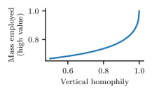
Figure 6: The parameter values are: $n_{H}=n_{L}=1$ so that $n=2$. We plot the mass of high-value workers employed in steady state as a function of the degree of value-homophily, $\alpha$.

We remark that value-homophily increases productivity, since in this example the mass of high valued workers translates directly into the overall productivity.

References

- (1)
- Arbex et al. (2019) Arbex, Marcelo, Dennis O’Dea, and David Wiczer, “Network search: Climbing the job ladder faster,” International Economic Review, 2019, 60 (2), 693–720.
- Arrow and Borzekowski (2004) Arrow, Kenneth J. and Ron Borzekowski, “Limited network connections and the distribution of wages,” FEDS Working Paper, 2004.
- Beaman (2012) Beaman, Lori A., “Social Networks and the Dynamics of Labour Market Outcomes: Evidence from Refugees Resettled in the U.S.,” Review of Economic Studies, 2012, 79 (1), 128–161.
- Beaman and Magruder (2012) and Jeremy Magruder, “Who gets the job referral? Evidence from a social networks experiment,” American Economic Review, 2012, 102 (7), 3574–3593.
- Beaman et al. (2018) Beaman, Lori, Niall Keleher, and Jeremy Magruder, “Do job networks disadvantage women? Evidence from a recruitment experiment in Malawi,” Journal of Labor Economics, 2018, 36 (1), 121–157.
- Benson et al. (2019) Benson, Alan, Simon Board, and Moritz Meyer ter Vehn, “Discrimination in hiring: Evidence from retail sales,” preprint: UCLA, 2019.
- Bond and Fernandez (2019a) Bond, Brittany M and Roberto M Fernandez, “Networks for the unemployed?,” Social Networks at Work, 2019.
- Bond and Fernandez (2019b) Bond, Brittany M. and Roberto M. Fernandez, “Networks for the unemployed?,” Social Networks at Work, 2019.
- Brown et al. (2016) Brown, Meta, Elizabeth Setren, and Giorgio Topa, “Do Informal Referrals Lead to Better Matches? Evidence from a Firm’s Employee Referral System,” Journal of Labor Economics, 2016, 34 (1), 161 – 209.
- Burks et al. (2015) Burks, Stephen V, Bo Cowgill, Mitchell Hoffman, and Michael Housman, “The value of hiring through employee referrals,” The Quarterly Journal of Economics, 2015, 130 (2), 805–839.