Incentivizing Routing Choices for Safe and Efficient Transportation in the Face of the COVID-19 Pandemic

Abstract.

The COVID-19 pandemic has severely affected many aspects of people’s daily lives. While many countries are in a re-opening stage, some effects of the pandemic on people’s behaviors are expected to last much longer, including how they choose between different transport options. Experts predict considerably delayed recovery of the public transport options, as people try to avoid crowded places. In turn, significant increases in traffic congestion are expected, since people are likely to prefer using their own vehicles or taxis as opposed to riskier and more crowded options such as the railway. In this paper, we propose to use financial incentives to set the tradeoff between risk of infection and congestion to achieve safe and efficient transportation networks. To this end, we formulate a network optimization problem to optimize taxi fares. For our framework to be useful in various cities and times of the day without much designer effort, we also propose a data-driven approach to learn human preferences about transport options, which is then used in our taxi fare optimization. Our user studies and simulation experiments show our framework is able to minimize congestion and risk of infection.

Figure 1. The cartoons depict an example of a transportation network we investigate in this paper. People use four different modes of transportation: private cars (green), taxis (yellow), railway, and walking. On the right, people avoid using public transportation modes (railway in this case) due to the effects of pandemic. In addition to more people having to walk, more private cars and taxis operate in the network, which increases traffic congestion and travel delays for everyone.

1. Introduction

As months go by, most of the world is still experiencing difficulties caused by the COVID-19 pandemic. With many governments pushing towards re-opening, experts predict more severe traffic congestion than before the pandemic (Carpenter, 2020), especially in urban cities that rely much on public transportation (Hu et al., 2020a). For example, studies suggest that in San Francisco, commuters will experience an additional round-trip delay of 20–80 minutes per person, at a societal cost of 556,000 – 2,736,000 added traffic hours per day (Hu et al., 2020b).

One of the main reasons for expecting such a dramatic increase in traffic congestion is because the inhabitants of large metropolitan areas remain reluctant to use public transport (Hertzke et al., 2020), and transportation engineers predict a similar trend to continue for a long period of time (Ewoldsen, 2020; Pedersen, 2020). In fact, large-scale user surveys that aggregate responses from different countries show, for both business and private trips, risk of infection has become the primary deciding factor on people’s choice of the mode of transportation, becoming more important than time to destination, price of trip, avoidance of congestion, convenience, space, and privacy as compared to pre-pandemic conditions (Hattrup-Silberberg et al., 2020). Accordingly, the use of public transportation has substantially declined (Tirachini and Cats, 2020). While there has also been a drastic decrease in the use of private vehicles due to lockdowns, the decline has been much more drastic for public transportation (Hertzke et al., 2020), and mobility data show the recovery with re-opening takes much longer for public transportation (Pascale, 2020). A similar shift away from ride-hailing services (Vitale et al., 2020) and taxis (Zheng et al., 2020) is also expected, adding more challenges to post-pandemic traffic congestion.

While “work from home” practices that have become more common during the pandemic help decrease the congestion for now (Kahaner, 2020), many metropolitan cities have started to take other precautions to avoid significant increases in traffic congestion as well as to mitigate the risk of infection. For example, London and Paris have embarked on plans to create more biking and walking lanes and routes (Hu and Schweber, 2020), whereas Istanbul implemented a model of alternate working hours for public servants and schools (Republic of Turkey Governorship of Istanbul, 2020). While different solutions may be applicable based on cultural factors or geographical conditions, researchers and experts emphasize financial incentives may play an important role for the recovery of public transportation and ride-hailing services (Teale, 2020). To achieve this, we need to address the challenge of modeling how human preferences have evolved through the pandemic, and how these new preferences should affect routing and pricing public transportation and ride-hailing services.

Our insight in this paper is that we can leverage data-driven techniques to learn how humans’ choices of mode of transportation have changed due to the pandemic, which we can use to optimize transportation networks in order to mitigate infection risk and decrease delays due to congestion. By modeling the network with four modes of transportation, namely private cars, taxis (or vehicles of ride-hailing services), railway, and pedestrians, we optimize the taxi fares based on total demand and other network properties for a social objective consisting of two factors: safety and efficiency. The users of the network choose their mode of transportation and the routes selfishly, i.e., they choose the route that will minimize their own latency, monetary cost and risk of infection.

Our model can be seen as an indirect Stackelberg game (Swamy, 2012; Krichene et al., 2018), where our planner first indirectly influences the demand for cars, taxis and railway by deciding the taxi fares. Then the humans respond selfishly by taking the highest-utility route available to them, where they might be optimizing based on their own priorities for latency, monetary cost, and risk of infection. Such a control scheme using financial incentives has previously been shown effective for mixed-autonomy traffic where regular and autonomous vehicles co-exist (Bıyık et al., 2019).

In order for our planning module to take into account people’s preferences about the mode of transportation, we learn how people tradeoff latency, price and risk of infection using preference-based learning. We adopt active learning techniques to improve data-efficiency, as the human is in-the-loop. Our user study results demonstrate that people care more about the risk of infection while choosing their transport post-pandemic. In addition, our results on a simulated traffic network shows our network optimization can be utilized to set the tradeoff between congestion and the risk of infection.

Our contributions in this work are three-fold:

• We study different modes of transportation in traffic networks by modeling their latencies and risks of infection.

• We leverage active preference-based learning techniques to learn humans’ preferences about the transport options while taking latency, monetary cost and the risk of infection into account.

• We formulate an optimization to set the taxi fares in the network, which uses the learned human preferences, to minimize traffic congestion and the risk of infection.

2. Related Work

We now overview the works that study modeling traffic under pandemic, routing games and pricing in transportation.

Traffic under Pandemic. Several works investigated the impact of the pandemic on transportation networks. Wang et al. (2020) analyzed the Multiscale Dynamic Human Mobility Flow Dataset (Kang et al., 2020) and Google Trends to investigate the correlation between the change of mobility patterns, government policies, and people’s awareness in the United States. Cui et al. (2020) proposed a traffic performance score to measure the impact of the pandemic on urban mobility. Tirachini and Cats (2020) pointed out the problems regarding public transportation due to the pandemic, and urged authorities for further research in order to sustain the benefits of public transportation. More related to our work, Hu et al. (2020a) and Zheng et al. (2020) showed the pandemic caused a change in the preferred transportation modes and the decline in the use of public transport may lead to worse traffic congestion than before. While all of these works are important to understand the scale of the problem and motivate our work, they do not propose a solution for achieving safe and efficient mobility under the pandemic.

Routing Games. Previous works in traffic optimization have formulated the routing problem as a game between drivers. Krichene et al. (2018) developed an algorithm for efficiently finding Nash equilibria, where drivers have no incentive to unilaterally deviate from their route choice, in parallel traffic networks under a single mode of transportation. Prior to that, Roughgarden and Tardos (2002) and Correa et al. (2008) had formalized how bad the Nash equilibrium can be in a routing game. In this paper, we focus on a setting where owners of private cars reach a Nash equilibrium, whereas the routing of taxis are indirectly controlled by a social planner through pricing. This is similar to the altruistic Nash equilibrium proposed by Bıyık et al. (2018), except we do not make altruism assumptions, but use financial incentives to attain the benefits of altruism. Lazar et al. (2019a) used reinforcement learning to solve Stackelberg routing games with mixed-autonomy where the planner had full control over the autonomous vehicles. Most relatedly, Bıyık et al. (2019) considered a similar setup in parallel networks where some portion of the traffic flow is indirectly controlled through pricing and the rest choose their routes selfishly. In this work, we extend the model to include public transportation (trains in particular) and incorporate safety measures due to the impacts of the pandemic, creating a more complex social objective.

Pricing in Transportation Networks. Our work is also related to the research in tolling (Beckmann et al., 1955), as we use financial incentives to enhance safety and efficiency. Specifically, Fleischer et al. (2004) and Brown and Marden (2016) studied tolling while taking the users’ various preferences into account. Sandholm (2002) derived tolls to have drivers choose socially optimal strategies. In the framework we consider in this work, train fares are constant and the pricing scheme is only for taxis that take various routes, rather than tolling.

Learning Humans’ Routing Preferences. Finally, our work leverages preference-based learning which enable learning humans’ preferences in the absence of user demonstrations (Sadigh et al., 2017; Kallus and Udell, 2016; Zadimoghaddam and Roth, 2012). In preference-based learning, the user is queried with a set of options from which they are asked to select the option they most like. While Bıyık et al. (2019) used preference-based learning with the volume removal objective to actively generate the queries, we adopt the information gain objective (Bıyık et al., 2020), which has been shown to be more data-efficient and user-friendly in terms of the easiness of queries.

3. Transportation Network Model

We begin by presenting the framework we use to model the traffic network we consider in this paper, as well as the monetary cost and risk of infection associated with each transportation mode. Our traffic network has one origin-destination (O-D) pair and multiple parallel roads that connect them. Roads are shared between private cars and taxis. Additionally, a railroad and pedestrian walking path connect the origin and destination. This is visualized in Fig. 1.

Our goal is to optimize the taxi fares, which depend on the route taken, to influence the state of the traffic to decrease latency and risk of infection. While optimizing taxi fares, our framework will also estimate the latency and risk of infection associated with each transport option. These estimations are then revealed to the commuters so that they can take these factors into account while choosing their transport option. In addition to the mode of transportation, people also choose their routes, i.e. they do not only choose to take a taxi, but also which route the taxi should take; because this has a direct effect on the fare they will pay. Such a solution can be feasible especially in ride-hailing services where customers choose their transport option prior to calling a vehicle.

There is an important tradeoff in our optimization: if taxi fares are too high, then more people may choose to take the train. While this decreases traffic congestion, high population density in the train may increase the risk of infection. On the other hand, too low taxi rates will hinder the recovery of public transport, increasing the traffic congestion. In addition to this tradeoff, allowing different fares for taxis based on the road they are taking gives more opportunities while still being fair to the customers: they can be financially incentivized with lower fares to take longer roads, which may keep the congestion low by preventing the quickest roads from being overused.

To formulate our optimization for taxi fares, we elaborate on each transportation medium in the subsequent sections.

3.1. Roads

We consider $n$ parallel roads and use $[n]=\{1,2,\ldots,n\}$ to denote the set of all roads. We denote the free-flow latency of road $i$, the time it takes to drive from origin to destination without any congestion, by $a_{i}$.

Latency. Private cars and taxis share the roads, so they both contribute to road congestion. The latency of a road depends on how many vehicles are using it. We use the traffic model proposed by the Bureau of Public Roads (BPR model) (of Public Roads, 1964; Daskin, 1985) to mathematically formulate this latency. This model has been widely used in literature for traffic management (Dowling et al., 1998), simulations (Florian and Nguyen, 1976), urban-scale analysis (Wong and Wong, 2016; Kucharski and Drabicki, 2017), and modeling mixed-autonomy traffic (Mehr and Horowitz, 2019; Lazar et al., 2020, 2019b).

We let $f_{i}^{c}$ denote the flow of private cars on road $i$, i.e., the number of private cars who use road $i$ per unit time. Similarly, $f_{i}^{t}$ denotes the flow of taxis on road $i$. Then the total flow of vehicles on road $i$ is $f_{i}^{v}=f_{i}^{c}+f_{i}^{t}$. According to the BPR model, the latency of this road is

(1) $$\ell_{i}^{v}(f_{i}^{v})=a_{i}\Big{[}1+\alpha\Big{(}\frac{f_{i}^{v}}{c_{i}}\Big{)}^{\beta}\Big{]}\>,$$

where $a_{i}$ and $c_{i}$ are constants denoting the free-flow latency and capacity of the road, respectively, and $\alpha,\beta\in\mathbb{R}_{>0}$ are the parameters of the BPR model. The capacity $c_{i}$ is proportional to the length and number of lanes of the road.

We then write the aggregate latency incurred per unit time on road $i$ and over the entire network as:

(2) $$L_{i}^{v}(f_{i}^{v})=f_{i}^{v}\cdot\ell_{i}^{v}(f_{i}^{v})\>,$$

(3) $$L^{v}(\bm{f}^{v})=\sum_{i\in[n]}L_{i}^{v}(f_{i}^{v})\>,$$

respectively, where $\bm{f}^{v}$ is the vector that consists of $f^{v}_{i}$ for $i=1,2,\dots,n$. This is total latency incurred per unit time, because $f_{i}^{v}$ denotes the flow, i.e., number of people per unit time, using road $i$.

Monetary Cost. Our goal is to optimize taxi fares for each road. We denote these fares as $x_{i}^{t}$ for $i\in[n]$. On the other hand, we do not assume any control over the monetary cost of traveling with private cars, due to gas prices, tolling, etc. We neglect the deviations on the cost due to the effect of congestion on gas prices, and assume the cost is only affected by the characteristics of the road, e.g., its length and nominal vehicle speed. Therefore, $x_{i}^{c}$ is a constant for the monetary cost of taking road $i$ with a private car.

Risk of Infection. Private cars do not pose an extra threat in terms of infection, because they do not create new close interactions between people. On the other hand, taxis create an interaction between the passenger and the driver. Therefore, while the risk of infection is $0$ for private cars, we let $\bar{r}^{t}$ denote the risk of infection per unit time for a single taxi. This value is affected by many factors that vary from city to city: the size and ventilation of taxis, whether there is a protective shield between the driver and the passenger, etc. And what is important is the ratio between $\bar{r}^{t}$ and the risk of infection in other transportation modes. Therefore, to keep our model general, we do not make additional assumptions about $\bar{r}^{t}$, which should be decided by health authorities.

Since longer interactions increase the risk, we model the total risk of infection a taxi causes during a trip on road $i$ as

(4) $$r_{i}^{t}(f_{i}^{v})=\bar{r}^{t}\cdot\ell_{i}^{v}(f_{i}^{v})\>,$$

and total risk over the network per unit time due to taxis as

(5) $$R^{t}(\bm{f}^{v})=\sum_{i\in[n]}f_{i}^{t}\cdot r_{i}^{t}=\sum_{i\in[n]}f_{i}^{t}\cdot\bar{r}^{t}\cdot\ell_{i}^{v}(f_{i}^{v})\>.$$

This is per unit time, because $f_{i}^{t}$ denotes the flow, i.e., number of people per unit time, using taxis.

Having modeled the roads, we now continue with the railway in our transportation network.

3.2. Railway

Our network includes a railway from the origin to the destination for the train option. Railways have a physical capacity that determines at most how many people can take trains per unit time. We let this capacity be $c^{r}$. We then define $f^{r}$ as the flow of people using the train, such that $0\leq f^{r}\leq c^{r}$ must be satisfied.

Latency. Since trains operate on a schedule, the latency of a train is affected by neither how congested the roads are nor the number of people taking the train. Using railway from origin to destination takes a duration of constant $\ell^{r}$. Similar to roads, we can write the aggregate latency incurred per unit time on the railway as

(6) $$L^{r}(f^{r})=f^{r}\cdot\ell^{r}.$$

Monetary Cost. Although the fares of taxis can be dynamically optimized based on the demand, railway has a fixed fare. We let $x^{r}$ denote the fare of the railway.

Risk of Infection. A very crucial aspect of the railway is that it may cause high risk of infection depending on how many people are aboard. We let $\bar{r}^{r}$ denote the total risk of infection per unit time per person on a railway that operates at full capacity, i.e., when $f^{r}=c^{r}$. Again letting health authorities decide $\bar{r}^{r}$ (relative to $r^{t}$), we can model the risk of infection per person during one trip in the railway as

(7) $$r^{r}(f^{r})=\ell^{r}\cdot\bar{r}^{r}\cdot\frac{f^{r}}{c^{r}}\>.$$

The total risk of infection due to the railway per unit time is then written as

(8) $$R^{r}(f^{r})=f^{r}\cdot r^{r}(f^{r})=\ell^{r}\cdot\bar{r}^{r}\cdot\frac{{f^{r}}^{2}}{c^{r}}\>.$$

Next, we proceed to the model of the walking path to finalize our transportation network model.

3.3. Walking Path

Our network has a walking path from origin to destination for people who do not want to use the other modes of transport. We denote the flow of these people, pedestrians, as $f^{p}$. While we use a simple model for pedestrians, it again poses the same latency-risk tradeoff: having many people walk will reduce both the risk (compared to taxis and railway) and the congestion in the roads, but is not a desirable scenario, as pedestrians themselves will experience huge delays.

Latency. Dividing the path length by the average human walking speed, we assume the latency of a pedestrian is a constant, denoted by $\ell^{p}$. The aggregate latency incurred per unit time on the walking path is then

(9) $$L^{p}(f^{p})=f^{p}\cdot\ell^{p}\>.$$

Monetary Cost. There is no monetary cost associated with walking to the destination.

Risk of Infection. The risk of infection for pedestrians depends on many external factors. For example, it increases if there are crowded places on the path, or it may decrease if policies enforce people to practice social distancing and wear face coverings. We denote the risk of infection per person per unit time on the path as $\bar{r}^{p}$, and so the total risk of infection per person on the walking path is $r^{p}=\ell^{p}\cdot\bar{r}^{p}$, and the total risk over the network per unit time is

(10) $$R^{p}(f^{p})=f^{p}\cdot r^{p}\>.$$

Having modeled all the mediums in our network, we are now ready to formulate the optimization problem for taxi fares in order to influence routing decisions of people and bring down the total latency and risk of infection.

4. Optimizing Safety & Efficiency

We first start with formulating our optimization objective, and then the constraints. Finally in Section 4.3, we present the overall optimization problem.

4.1. Objective

Our goal is to optimize the taxi fares such that all people in the network will experience both low risk of infection and low latency. The network model we presented in Section 3 allows us to model these two objectives:

(11) Latency: $$L(\bm{f}^{v},f^{r},f^{p})=L^{v}(\bm{f}^{v})+L^{r}(f^{r})+L^{p}(f^{p})\>,$$

(12) Risk: $$R(\bm{f}^{v},f^{r},f^{p})=R^{v}(\bm{f}^{v})+R^{r}(f^{r})+R^{p}(f^{p})\>,$$

Our problem is then a multi-objective optimization where we try to minimize a weighted sum of (11) and (12). Next, we formulate the constraints of our optimization.

4.2. Constraints

Fare Constraints. While we assume the city planner determines the taxi fares, we still need to make sure taxi drivers make profit, so we cannot set the fares arbitrarily low.

One can think of a solution where some minimum profit constraint is imposed over the entire network (similar to (Bıyık et al., 2019)). However, this requires some centralization to balance the profits because the optimization may produce very low fares for longer roads and high fares for shorter roads to satisfy the profit constraint. In such a case, the taxis operating on the shorter roads would make a lot of profit while the other taxis are losing money. As taxis are usually decentralized, it is not realistic to assume a central authority will compensate the taxi drivers who lose money by taxing the ones who make more profit. This can, however, be an interesting direction for ride-hailing apps which naturally have a centralized system.

In this work, we instead impose the fare constraints separately for each road to make sure all taxis make profit. For this, we impose a minimum fare $x^{t}_{i}\geq\bar{x}^{t}_{i}$ for each road $i\in[n]$ where $\bar{x}^{t}_{i}$ can be determined by how much minimum profit is desired for each trip on road $i$. One can think of $\bar{x}^{t}_{i}$ proportional to $\bar{x}^{c}_{i}$, depending on gas-efficiency of the taxis.

Flow Constraints. While we can financially incentivize people to take different modes of transportation by optimizing taxi fares, we cannot explicitly force them to take a particular mode. Hence, we are constrained by their preferences. To model humans’ choices of the mode of transportation, we let $\bm{h}$ be a discrete probability distribution over $2n+2$ transport options: $n$ options with private cars, $n$ with taxis, $1$ with the railway and $1$ as a pedestrian. The vector $\bm{h}$ sums up to one and consists of the following terms: $h^{c}_{i}$ for $i\in[n]$, $h^{t}_{i}$ for $i\in[n]$, $h^{r}$ and $h^{p}$. Each of these represents what fraction of the total flow chooses the corresponding transport option.

The vector $\bm{h}$ of course depends on the latencies, monetary costs and the risks of infection of all transport options. Hence, we let it be a function: $\bm{h}(\bm{\ell},\bm{x},\bm{r})$. Here $\bm{\ell}$, $\bm{x}$ and $\bm{r}$ denote the vectors that consist of the latency, monetary cost and risk of infection, respectively, for all transport options. For now, we treat the preference distribution $\bm{h}(\bm{\ell},\bm{x},\bm{r})$ as a black-box function to complete our optimization formulation, and defer its derivation to Section 5.

4.3. Overall Optimization Problem

Letting $F$ denote the total demand per unit time, we can write the overall optimization problem as:

(13) $$\begin{split}\min_{\bm{x}^{t}}\;&\gamma\cdot R(\bm{f}^{v},f^{r},f^{p})+(1-\gamma)\cdot L(\bm{f}^{v},f^{r},f^{p})\\ \textrm{subject to }\;&x^{t}_{i}\geq\bar{x}^{t}_{i}\quad\forall i\in[n]\>,\\ &\ell_{i}^{c}=\ell_{i}^{t}=a_{i}\Big{[}1+\alpha\Big{(}\frac{f_{i}^{c}+f_{i}^{t}}{c_{i}}\Big{)}^{\beta}\Big{]}\quad\forall i\in[n]\>,\\ &r^{r}=\ell^{r}\cdot\bar{r}^{r}\cdot\frac{f^{r}}{c^{r}}\>,\quad r^{p}=\ell^{p}\cdot\bar{r}^{p}\>,\\ &r_{i}^{t}=\bar{r}^{t}\cdot\ell_{i}^{v}\quad\forall i\in[n]\>,\\ &f_{i}^{c}=F\cdot h_{i}^{c}(\bm{\ell},\bm{x},\bm{r})\quad\forall i\in[n]\>,\\ &f_{i}^{t}=F\cdot h_{i}^{t}(\bm{\ell},\bm{x},\bm{r})\quad\forall i\in[n]\>,\\ &f^{r}=F\cdot h^{r}(\bm{\ell},\bm{x},\bm{r})\leq c^{r}\>,\\ &f^{p}=F\cdot h^{p}(\bm{\ell},\bm{x},\bm{r})\>,\end{split}$$

where $0\leq\gamma\leq 1$ is a weight that determines the relative importance of the latency and risk objectives.

5. Preference Distribution Model

The only missing component in our optimization is how we model the preference distribution $\bm{h}(\bm{\ell},\bm{x},\bm{r})$. While all humans will presumably choose transport options to minimize their latency, monetary cost, and risk of infection, their tradeoff between these factors differ: some people prioritize minimizing their monetary cost whereas some prioritize reaching their destination as early as possible. Moreover, people may have other biases. For example, one may prefer taking a taxi rather than driving a car so that they can read during the trip, or one may prefer walking to stay healthy.

To incorporate such preferences, we model humans as agents optimizing a utility function that captures their preferences. For this, we first assume humans will not choose dominated options, i.e., options that have no advantage over some other option and have at least one disadvantage. Formally, option $j$, denoted by $o_{j}$, is dominated by $o_{j^{\prime}}$ if:

$$o_{j}\textit{ and }o_{j^{\prime}}\textit{ are the same mode of transportation, }\textrm{and}$$

(14) $$\left(\ell_{j^{\prime}}\leq\ell_{j}\>\land\>x_{j^{\prime}}\leq x_{j}\>\land\>r_{j^{\prime}}\leq r_{j}\right),\textrm{ and}$$

$$\left(\ell_{j^{\prime}}<\ell_{j}\>\lor\>x_{j^{\prime}}<x_{j}\>\lor\>r_{j^{\prime}}<r_{j}\right)\>,$$

where $\ell_{j}$, $x_{j}$ and $r_{j}$ represent the latency, monetary cost and the risk of option $o_{j}$, respectively, and similarly $\ell_{j^{\prime}}$, $x_{j^{\prime}}$ and $r_{j^{\prime}}$ represent those of option $o_{j^{\prime}}$. Note that the railway and the walking path cannot be dominated as there is only one option each for them. The set of dominated options can be written as:

(15) $$\begin{split}D&=\{o_{j}\mid o_{j^{\prime}}\textrm{ dominates }o_{j}\text{ for some option }o_{j^{\prime}}\}\>,\end{split}$$

Then, we model the utility of a human user, parameterized by $\bm{\omega}\in\mathbb{R}^{7}$, as:

(16) $$\begin{split}u_{\bm{\omega}}(o_{j})=\omega_{1}&\ell_{j}+\omega_{2}x_{j}+\omega_{3}r_{j}+\\ &\begin{cases}-\infty,\;\textrm{ if }o_{j}\in D,\\ \omega_{4},\;\textrm{ if }o_{j}\textrm{ is private car and }o_{j}\not\in D,\\ \omega_{5},\;\textrm{ if }o_{j}\textrm{ is taxi and }o_{j}\not\in D,\\ \omega_{6},\;\textrm{ if }o_{j}\textrm{ is railway},\\ \omega_{7},\;\textrm{ if }o_{j}\textrm{ is walking path}\end{cases},\end{split}$$

where $o_{j}$ denotes the chosen transport option. Here, the first three elements of $\bm{\omega}$ characterize the tradeoff between the three factors of latency, cost, and risk, whereas the last four model humans’ biases towards the different modes of transportation. Presumably, the first three elements of $\bm{\omega}$ must be negative, penalizing high latency, cost and risk, for all humans. Such linear utility functions are common in preference-based learning as they are expressive enough to capture most of the important information (Wilde et al., 2020; Bıyık et al., 2020; Sadigh et al., 2017). Extensions to nonlinear models are possible with the use of Gaussian processes (Biyik et al., 2020).

Having defined a utility function for a human whose preferences are encoded with a vector $\bm{\omega}$, we now adopt a widely-used probabilistic model from discrete choice theory to calculate the probability of the human choosing each option: multinomial logit model (Ben-Akiva and Lerman, 2018). This model has been extensively used both in transportation engineering (Koppelman, 1983; Bıyık et al., 2019) and preference-based learning (Sadigh et al., 2017; Bıyık et al., 2020). According to this model, the probability of the human choosing $o_{j}$ among all options available to them, $\mathcal{O}$, is:

(17) $$P_{\bm{\omega}}(o_{j}\mid\mathcal{O})=\frac{\exp(u_{\bm{\omega}}(o_{j}))}{\sum_{o_{j^{\prime}}\in\mathcal{O}}\exp(u_{\bm{\omega}}(o_{j^{\prime}}))}\>.$$

This model makes sure the dominated options have $0$ probability of being chosen, as their utilities are $-\infty$. Moreover, this model allows us to handle users with different transport options. For example, $\mathcal{O}$ may or may not include the private car option, depending on whether the user owns a car or not. We let $\mathcal{O}_{k}$ denote the options available to the user $k$.

We also let $g_{k}$ denote the distribution over user $k$’s preferences, i.e. their preference vector $\bm{\omega}$. Then, the preference distribution $\bm{h}(\bm{\ell},\bm{x},\bm{r})$ of the entire population of users can be written as:

(18) $$h_{j}(\bm{\ell},\bm{x},\bm{r})=\frac{1}{N}\sum_{k=1}^{N}\int_{\mathbb{R}^{7}}P_{\bm{\omega}}(o_{j}\mid\mathcal{O}_{k})g_{k}(\bm{\omega})d\bm{\omega}$$

for each transport option $j$, where $N$ is the population. This computation can be efficiently performed via sampling from $g_{k}$’s using, for example, Metropolis-Hastings algorithm.

In the next section, we discuss how data-driven methods can be leveraged to learn the distributions $g_{k}$, which will then complete our framework.

6. Learning User Preferences

We take a Bayesian approach to learn the distributions $g_{k}$ of humans’ preferences. In this approach, there exists a data set for each human that consists of their selected option as well as the options that were available to them while making their choice. While one can combine all data sets to learn a single $g$, learning a distribution for each human is advantageous, because this allows further personalizing our model to specific populations, such as people who travel in the early morning or later in the day. For example, people traveling early in the morning might care more about latency on their way to work, whereas travelers who leave later in the day may want to enjoy some nice weather by walking. Therefore, we learn a separate distribution for each user, and $g$ is simply the average of such distributions associated with the humans traveling at that time.

Given a data sample for human $k$ where they chose option $o_{j}$ among available options $\mathcal{O}_{k}$, we use Bayes’ rule to update the posterior $g_{k}$:

(19) $$g_{k}\left(\bm{\omega}\mid o_{j},\mathcal{O}_{k}\right)\propto g_{k}(\bm{\omega})P_{\bm{\omega}}(o_{j}\mid\mathcal{O}_{k})\>.$$

Assuming conditional independence of different choices, the posterior learned with the full data set of the human $k$ is:

(20) $$g_{k}\left(\bm{\omega}\mid\mathcal{D}\right)\propto g_{k}(\bm{\omega})\prod_{(o_{j}\mid\mathcal{O}_{k})\in\mathcal{D}}P_{\bm{\omega}}(o_{j}\mid\mathcal{O}_{k})\>,$$

where $\mathcal{D}$ denotes the data set.

This learning approach yields better estimates of $g_{k}$ as we collect more data of human $k$. While we can generate more data by running our optimization in (13) on real network instances, this optimization is only designed to optimize for taxi fares and is not designed for optimally collecting data from humans for learning their preferences. Hence, it does not necessarily generate queries (transport options) that will lead to significant improvements in our estimates of $g_{k}$, which may, in turn, hurt the performance of network optimization. To overcome this problem, we present an optional active querying method based on information gain in the subsequent section, which optimizes the queries, i.e. their latencies, monetary costs and risks without necessarily satisfying the network dynamics to learn the humans’ preferences optimally. Such an approach could be employed in practice by, for example, having a survey for humans who enter the network for the first time.

6.1. Active Querying

To enable faster learning of $g_{k}$, we use an active learning method that optimizes the information gained from each query about the distribution $g_{k}$ of $\bm{\omega}$. While prior works used a volume removal based active learning approach where the goal is to maximize the volume removed from the distribution $g_{k}$ (Sadigh et al., 2017; Bıyık et al., 2019; Golovin and Krause, 2011), Bıyık et al. (2020) showed maximizing mutual information leads to both faster learning and easier queries for the humans. In this method, each query is optimized after receiving the human’s choice:

(21) $$\max_{\mathcal{O}_{k}}I(\bm{\omega};o_{j}\mid\mathcal{O}_{k})\!=\!\max_{\mathcal{O}_{k}}\!\left[H(\bm{\omega}\mid\mathcal{O}_{k})\!-\!\mathbb{E}_{o_{j}}\!\left[H(\bm{\omega}\mid o_{j},\mathcal{O}_{k})\right]\right],$$

where $I$ is the mutual information, $H$ is the information entropy (Cover, 1999), and $o_{j}$ is the random variable representing the selected transport option. After sampling $\bm{\omega}\sim g_{k}(\bm{\omega})$ and letting the set of samples be $\Omega$, the optimization (21) is asymptotically equal to

(22) $$\max_{\mathcal{O}_{k}}\sum_{o_{j}\in\mathcal{O}_{k}}\sum_{\bm{\omega}\in\Omega}P_{\bm{\omega}}(o_{j}\mid\mathcal{O}_{k})\log\frac{P_{\bm{\omega}}(o_{j}\mid\mathcal{O}_{k})}{\sum_{\bm{\omega}^{\prime}\in\Omega}P_{\bm{\omega}^{\prime}}(o_{j}\mid\mathcal{O}_{k})}$$

as the number of $\bm{\omega}$ samples in $\Omega$ goes to infinity. We refer to (Bıyık et al., 2020) for the full derivation.

We want to note again that this optimization is not subject to the constraints of the optimization we presented in (13), because the goal here is to learn the user preferences as quickly as possible using some artificial queries that ask the users about their transportation preferences.

Having presented our approach to learn humans’ preferences over transport options and our active querying approach to accelerate learning, our framework is complete.

7. Experiments & Results

In this section, we present our experiments and the results. We divide the experiments into two parts: a user study where we learn user preferences with the approach described in Section 6, and a case study on a simulated traffic network where we optimize the taxi fares as formulated in Section 4 using the preferences learned in the user study.

7.1. Learning User Preferences

To perform the optimization for a given traffic network, we first need to learn the distribution of humans’ preferences, $g_{k}$’s. For this, we surveyed 17 people across the United States during the second half of 2020, using the active learning framework we described in Section 6.1.

The participants were first explained the purpose of the survey, as well as the underlying model for calculating the risk of infection. Their place of residence, whether they were tested positive before for COVID-19, and their informed consent were collected. Each participant then answered $10$ actively generated queries, followed by $6$ queries that were randomly generated. We used the latter set of queries to test the accuracy of the predicted utility parameters $\bm{\omega}$: we looked at for how many of those queries our estimated $\bm{\omega}$’s could correctly predict the actual participant response. Each query consisted of $6$ choices —two roads with private cars and taxis, a railway, and a walking path. For the transport options, we provided the users with the estimated latencies, monetary costs and the estimated densities to give them an easily interpretable measure of infection risk.

To validate the impact of the pandemic on humans’ transport choices, we attempted to model the pre-pandemic distribution of people’s preferences, as well. For this, we asked the same participants to repeat the survey as if they were making their decisions prior to the pandemic. All 17 participants attended this second round survey.

The validation accuracy of our learning model is $97.1\%$ for pre-pandemic conditions, and $89.8\%$ for post-pandemic. As each query consisted of 6 transport options, these high accuracy values indicate we were able to accurately model participants’ preferences. The decrease in the accuracy from pre-pandemic to post-pandemic might be because risk of infection is less relevant in the pre-pandemic case, making the learning easier.

Using the preference data we collected, we generated two sets of preference distributions. Fig. 2 visualize the tradeoffs for each of the 17 study participants, where small points show the samples from their $g_{k}(\bm{\omega})$, and the mean of the distribution is indicated with a large point.

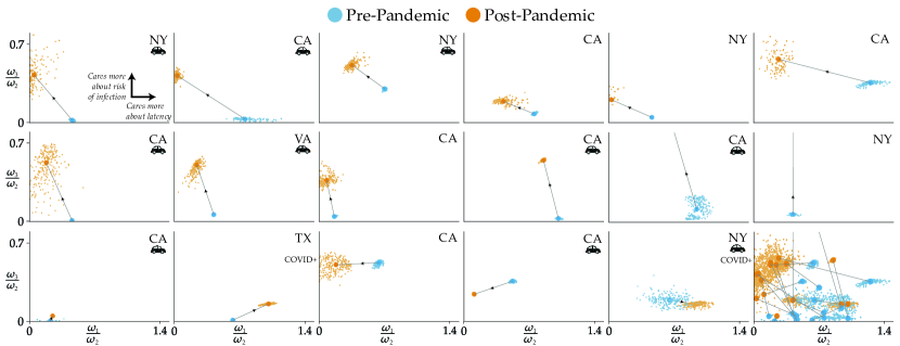
Figure 2. Distribution of participants’ learned tradeoff parameters. Their places of residence are noted on the top right of each plot (CA - California, NY - New York, VA - Virginia, TX - Texas). Two participants who were infected with COVID-19 before have also been labeled. Car icons indicate whether those participants were simulated as private car owners or not in Section 7.2. The bottom right plot shows all participants. It can be seen that $14$ of the $17$ participants care more about risk of infection in the post-pandemic case. The changes in the other three are much smaller.

We see from Fig. 2 how the pandemic affected humans’ relative tradeoffs between latency, monetary cost, and risk of infection. The majority of participants (14 out of 17) showed an increase in their regard for risk relative to monetary cost, and the changes in the other three are much smaller. This shows that people are putting a higher weight on the risk of infection associated with a travel option.

Moreover, the majority (13 out of 17) showed a decrease in their regard for latency relative to monetary cost. In the post-pandemic case, people are more willing to sacrifice their time for monetary considerations. This shows that our idea of using financial incentives to influence the state of the traffic network can in fact be effective.

It is interesting to point out that the only two participants whose preference ratios significantly moved rightward, i.e. who started caring more about latency, were the only two participants who were infected with and cured for COVID-19 prior to the surveys. This might be because they have less fear of being re-infected.

Having validated people are more concerned about the risk of infection, and shown the usability of our preference-based learning framework, we now proceed to the simulated traffic network experiments.

7.2. Case Study

To show the benefits of our optimization framework, we designed a case study with a traffic network consisting of four modes of transportation. The network we used is similar to the depiction given in Fig. 1, containing $n=2$ roads, a railway, and a walking path, all connecting one O-D pair.

The free-flow latencies of the two roads are $a_{1}=30$ minutes and $a_{2}=45$ minutes. Their capacities are $c_{1}=900$ and $c_{2}=600$ vehicles per minute. The monetary cost associated with driving a private car on these roads is $x_{1}^{c}=\$15$ and $x_{2}^{c}=\$9$. The minimum taxi fares for the two roads are $\bar{x}_{1}^{t}=\$9$ and $\bar{x}_{2}^{t}=\$5$. Road 1 can be thought of as a high-capacity, high-cost freeway option, while road 2 is a low-capacity, low-cost street. The train latency, capacity, and fare are $\ell^{r}=35$ minutes, $c^{r}=1500$ passengers per minute, and $x^{r}=\$3$ respectively. The walking path latency is $\ell^{p}=120$ minutes.

We set the parameters related to risk of infection in our simulated problem as follows. Risks of infection per minute for taxis and pedestrians are $\bar{r}^{t}=\bar{r}^{p}=1$. For the railway, we set the risk of a full capacity train (per minute) as $\bar{r}^{r}=10$.

The flow demand for this network is set to $F=3000$ people per minute. We simulated this population using the $\bm{\omega}$ samples we obtained from the user studies presented in Section 7.1. To separate the population of car-owners from the rest, as they will have different routing options $\mathcal{O}_{k}$, we simulated $10$ of the participants as car-owners. Those users are indicated with a car icon in Fig. 2.

We used a Sequential Quadratic Programming algorithm developed by (Kraft, 1988) to locally solve the optimization, and repeated with 100 random initializations to get closer to the global optimum. We performed this procedure for the two data sets (pre- and post-pandemic) as well as varying values of $\gamma$. Fig. 3 depicts the effect $\gamma$ has on the tradeoff between latency and risk of infection in our objective function. As expected, increasing $\gamma$ helps minimize risk of infection. The constraints enforced by users’ post-pandemic preferences put higher priority on risk of infection as opposed to latency, making aggregate risk of infection less sensitive to changes in $\gamma$. On the other hand, for pre-pandemic preferences, people’s disregard for risk and larger regard for latency make $\gamma$ have a larger effect on risk of infection as opposed to latency.

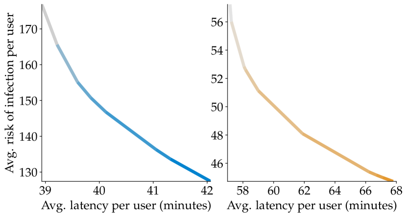
Figure 3. Optimized risk and latency tradeoff is shown for varying $\gamma$ under the pre-pandemic (left) and post-pandemic (right) conditions. Each value of $\gamma$ is used to generate a point on the plot, and line segments connecting adjacent points are colored to correspond with the values of $\gamma$. Darker colors correspond to higher $\gamma$. Higher $\gamma$ prioritizes minimizing risk of infection, at the cost of higher latencies.

Finally, Fig. 4 shows the specific solutions for three different $\gamma$ under pre-pandemic and post-pandemic conditions. Higher $\gamma$ leads to lower risk of infection by populating the railway less, whereas lower $\gamma$ decreases traffic congestion.

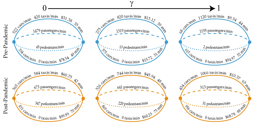
Figure 4. Solutions to the optimization for pre-pandemic (top) and post-pandemic (bottom) for varying $\gamma$ (increasing from left to right). The lines depict road 1, the railway, the walking path, and road 2 from top to bottom. As $\gamma$ increases, our framework fiscally incentivizes users to take the taxi on road $1$. This helps minimize the number of passengers on the railway, as well as the number of pedestrians on the walking path. Note that the price for a taxi on road $2$ does not have to follow a trend as $\gamma$ increases, but only has to stay higher than the price for a taxi on road $1$ so that it remains as a dominated option to make sure all the taxis go on road $1$.

8. Conclusion

Summary. We proposed a complete framework consisting of a learning and a planning module: we first learn humans’ transport preferences in a data-driven way using active preference-based learning. We then use these learned preferences to optimize taxi fares in traffic networks. Our user study results align with the expert predictions (Hu and Schweber, 2020) and larger-scale surveys (Hattrup-Silberberg et al., 2020), and simulation experiments demonstrate the usability and the benefits of the framework. Discussion. Due to the sensitive nature of the topic at hand, one should consider the moral implications that our results make. On the positive side, our results show that financial incentives can be used to decrease the risk of infection and accelerate the recovery of public transport. However, there is a natural tradeoff between these two objectives, which means hypothetically financial incentives could be used in ways that put riders at risk in order to recover public transport more quickly. Our goal here is not to advocate for such an approach, but to better understand people’s preferences. We hope that authorities take the necessary precautions to decrease infection risks under a certain level, and use financial incentives only afterwards to recover public transport.

Limitations and Future Work. In this paper, we studied traffic networks that consist of parallel roads and a single O-D pair. While this is a common assumption (as in (Bıyık et al., 2018; Krichene et al., 2018; Bıyık et al., 2019)), extensions to general network topologies remain as a future work: one can think of enumerating all possible paths from all origins to all destinations and then calculating the path latencies as the sum of corresponding roads’ latencies. In our case study, we considered a network with only two parallel roads for the clarity of presentation. While the real-world applications do not usually involve many parallel roads, our framework is scalable to the larger number of roads. Moreover, our user studies are limited due to the number of participants and the inherent bias people might have due to the pandemic while attending the pre-pandemic survey. Finally, we assumed the risk of infection is proportional to the interaction time in trains and taxis and for pedestrians. While this may not be accurate, our framework can be easily modified for better risk modeling.

References

- (1)
- Beckmann et al. (1955) Martin J Beckmann, Charles B McGuire, and Christopher B Winsten. 1955. Studies in the Economics of Transportation. (1955).
- Ben-Akiva and Lerman (2018) Moshe Ben-Akiva and Steven R Lerman. 2018. Discrete choice analysis: theory and application to travel demand. Transportation Studies.
- Biyik et al. (2020) Erdem Biyik, Nicolas Huynh, Mykel J. Kochenderfer, and Dorsa Sadigh. 2020. Active Preference-Based Gaussian Process Regression for Reward Learning. In Proceedings of Robotics: Science and Systems (RSS).
- Bıyık et al. (2018) Erdem Bıyık, Daniel A Lazar, Ramtin Pedarsani, and Dorsa Sadigh. 2018. Altruistic Autonomy: Beating Congestion on Shared Roads. In Workshop on Algorithmic Foundations of Robotics (WAFR).
- Bıyık et al. (2019) Erdem Bıyık, Daniel A. Lazar, Dorsa Sadigh, and Ramtin Pedarsani. 2019. The Green Choice: Learning and Influencing Human Decisions on Shared Roads. In Proceedings of the 58th IEEE Conference on Decision and Control (CDC).
- Bıyık et al. (2020) Erdem Bıyık, Malayandi Palan, Nicholas C. Landolfi, Dylan P. Losey, and Dorsa Sadigh. 2020. Asking Easy Questions: A User-Friendly Approach to Active Reward Learning (Proceedings of Machine Learning Research, Vol. 100), Leslie Pack Kaelbling, Danica Kragic, and Komei Sugiura (Eds.). PMLR, 1177–1190. http://proceedings.mlr.press/v100/b-iy-ik20a.html
- Brown and Marden (2016) Philip N Brown and Jason R Marden. 2016. The robustness of marginal-cost taxes in affine congestion games. IEEE Trans. Automat. Control 62, 8 (2016), 3999–4004.
- Carpenter (2020) Susan Carpenter. 2020. LA Traffic Could Be Worse Post Pandemic. Spectrum News 1 (Jul 2020). https://spectrumnews1.com/ca/la-west/transportation/2020/07/30/la-traffic-could-be-worse-post-pandemic
- Correa et al. (2008) José R Correa, Andreas S Schulz, and Nicolás E Stier-Moses. 2008. A geometric approach to the price of anarchy in nonatomic congestion games. Games and Economic Behavior 64, 2 (2008), 457–469.
- Cover (1999) Thomas M Cover. 1999. Elements of information theory. John Wiley & Sons.
- Cui et al. (2020) Zhiyong Cui, Meixin Zhu, Shuo Wang, Pengfei Wang, Yang Zhou, Qianxia Cao, Cole Kopca, and Yinhai Wang. 2020. Traffic Performance Score for Measuring the Impact of COVID-19 on Urban Mobility. arXiv preprint arXiv:2007.00648 (2020).
- Daskin (1985) Mark S Daskin. 1985. Urban transportation networks: Equilibrium analysis with mathematical programming methods.
- Dowling et al. (1998) Richard G Dowling, Rupinder Singh, and Willis Wei-Kuo Cheng. 1998. Accuracy and performance of improved speed-flow curves. Transportation research record 1646, 1 (1998), 9–17.
- Ewoldsen (2020) Beth Ewoldsen. 2020. COVID-19 Trends Impacting the Future of Transportation Planning and Research. National Academies of Sciences, Engineering, and Medicine (Aug 2020). https://www.nationalacademies.org/trb/blog/covid-19-trends-impacting-the-future-of-transportation-planning-and-research
- Fleischer et al. (2004) Lisa Fleischer, Kamal Jain, and Mohammad Mahdian. 2004. Tolls for heterogeneous selfish users in multicommodity networks and generalized congestion games. In 45th Annual IEEE Symposium on Foundations of Computer Science. IEEE, 277–285.
- Florian and Nguyen (1976) Michael Florian and Sang Nguyen. 1976. Recent experience with equilibrium methods for the study of a congested urban area. In Traffic Equilibrium Methods. Springer, 382–395.
- Golovin and Krause (2011) Daniel Golovin and Andreas Krause. 2011. Adaptive submodularity: Theory and applications in active learning and stochastic optimization. Journal of Artificial Intelligence Research 42 (2011), 427–486.
- Hattrup-Silberberg et al. (2020) Martin Hattrup-Silberberg, Saskia Hausler, Kersten Heineke, Nicholas Laverty, Timo Möller, Dennis Schwedhelm, and Ting Wu. 2020. Five COVID-19 aftershocks reshaping mobility’s future. McKinsey & Company (Sep 2020). https://www.mckinsey.com/industries/automotive-and-assembly/our-insights/five-covid-19-aftershocks-reshaping-mobilitys-future
- Hertzke et al. (2020) Patrick Hertzke, Simon Middleton, Guillaume Neu, and Henry Weaver. 2020. Moving forward: How COVID-19 will affect mobility in the United Kingdom. McKinsey & Company (June 2020). https://www.mckinsey.com/industries/automotive-and-assembly/our-insights/moving-forward-how-covid-19-will-affect-mobility-in-the-united-kingdom
- Hu and Schweber (2020) Winnie Hu and Nate Schweber. 2020. Will Cars Rule the Roads in Post-Pandemic New York? The New York Times (Aug 2020). https://www.nytimes.com/2020/08/10/nyregion/nyc-streets-parking-dining-busways.html
- Hu et al. (2020a) Yue Hu, William Barbour, Samitha Samaranayake, and Dan Work. 2020a. Impacts of Covid-19 mode shift on road traffic. arXiv preprint arXiv:2005.01610 (2020).
- Hu et al. (2020b) Yue Hu, Will Barbour, Samitha Samaranayake, and Dan Work. 2020b. The rebound — How Covid-19 could lead to worse traffic. Medium (Apr 2020). https://medium.com/@barbourww/the-rebound-how-covid-19-could-lead-to-worse-traffic-cb245a5b1da2
- Kahaner (2020) Larry Kahaner. 2020. Working from home a major factor in post-pandemic traffic. FleetOwner (Aug 2020). https://www.fleetowner.com/covid-19-coverage/article/21139861/working-from-home-a-major-factor-in-postpandemic-traffic
- Kallus and Udell (2016) Nathan Kallus and Madeleine Udell. 2016. Revealed preference at scale: Learning personalized preferences from assortment choices. In Proceedings of the 2016 ACM Conference on Economics and Computation. 821–837.
- Kang et al. (2020) Yuhao Kang, Song Gao, Yunlei Liang, Mingxiao Li, Jinmeng Rao, and Jake Kruse. 2020. Multiscale dynamic human mobility flow dataset in the us during the covid-19 epidemic. arXiv preprint arXiv:2008.12238 (2020).
- Koppelman (1983) Frank S Koppelman. 1983. Predicting transit ridership in response to transit service changes. Journal of Transportation Engineering 109, 4 (1983), 548–564.
- Kraft (1988) Dieter Kraft. 1988. A Software Package for Sequential Quadratic Programming. Technical Report. Institut für Dynamik der Flugsysteme Oberpfaffenhofen.
- Krichene et al. (2018) Walid Krichene, Jack D Reilly, Saurabh Amin, and Alexandre M Bayen. 2018. Stackelberg routing on parallel transportation networks. Handbook of Dynamic Game Theory (2018).
- Kucharski and Drabicki (2017) Rafał Kucharski and Arkadiusz Drabicki. 2017. Estimating macroscopic volume delay functions with the traffic density derived from measured speeds and flows. Journal of Advanced Transportation 2017 (2017).
- Lazar et al. (2020) Daniel Lazar, Samuel Coogan, and Ramtin Pedarsani. 2020. Routing for traffic networks with mixed autonomy. IEEE Trans. Automat. Control (2020).
- Lazar et al. (2019a) Daniel A Lazar, Erdem Bıyık, Dorsa Sadigh, and Ramtin Pedarsani. 2019a. Learning How to Dynamically Route Autonomous Vehicles on Shared Roads. arXiv preprint arXiv:1909.03664 (2019).
- Lazar et al. (2019b) Daniel A Lazar, Samuel Coogan, and Ramtin Pedarsani. 2019b. Optimal tolling for heterogeneous traffic networks with mixed autonomy. In 2019 IEEE 58th Conference on Decision and Control (CDC). IEEE, 4103–4108.
- Mehr and Horowitz (2019) Negar Mehr and Roberto Horowitz. 2019. How will the presence of autonomous vehicles affect the equilibrium state of traffic networks? IEEE Transactions on Control of Network Systems 7, 1 (2019), 96–105.
- of Public Roads (1964) United States. Bureau of Public Roads. 1964. Traffic assignment manual. US Department of Commerce, Bureau of Public Roads, Office of Planning, Urban Planning Division.
- Pascale (2020) Jordan Pascale. 2020. Here Are Four Charts That Show The Pandemic’s Impact On Locals’ Travel Habits. Wamu (Jul 2020). https://wamu.org/story/20/07/16/here-are-four-charts-that-show-the-pandemics-impact-on-locals-travel-habits/
- Pedersen (2020) Neil Pedersen. 2020. Impacts of COVID-19 on Transportation and Key Considerations for the Future. http://onlinepubs.trb.org/onlinepubs/PedersenITEAnnual%20Meeting200813.pptx Presentation at ITE 2020 Annual Meeting (Online).
- Republic of Turkey Governorship of Istanbul (2020) Republic of Turkey Governorship of Istanbul. 2020. Governor Yerlikaya Made a Press Release Regarding Gradual Working Hours Practice in Istanbul. (Sep 2020). http://en.istanbul.gov.tr/governor-yerlikaya-made-a-press-release-regarding-gradual-working-hours-practice-in-istanbul
- Roughgarden and Tardos (2002) Tim Roughgarden and Éva Tardos. 2002. How bad is selfish routing? Journal of the ACM (JACM) 49, 2 (2002), 236–259.
- Sadigh et al. (2017) Dorsa Sadigh, Anca D. Dragan, S. Shankar Sastry, and Sanjit A. Seshia. 2017. Active Preference-Based Learning of Reward Functions. In Proceedings of Robotics: Science and Systems (RSS).
- Sandholm (2002) William H Sandholm. 2002. Evolutionary implementation and congestion pricing. The Review of Economic Studies 69, 3 (2002), 667–689.
- Swamy (2012) Chaitanya Swamy. 2012. The effectiveness of Stackelberg strategies and tolls for network congestion games. ACM Transactions on Algorithms (TALG) 8, 4 (2012), 1–19.
- Teale (2020) Chris Teale. 2020. Transportation leaders focus on regaining trust before building anew. Smart Cities Dive (May 2020). https://www.smartcitiesdive.com/news/transportation-leaders-focus-on-regaining-trust-before-building-anew/577394
- Tirachini and Cats (2020) Alejandro Tirachini and Oded Cats. 2020. COVID-19 and public transportation: Current assessment, prospects, and research needs. Journal of Public Transportation 22, 1 (2020), 1.
- Vitale et al. (2020) Joe Vitale, Karen Bowman, and Ryan Robinson. 2020. How the pandemic is changing the future of automotive. Deloitte (Jul 2020). https://deloitte.com/us/en/insights/industry/retail-distribution/consumer-behavior-trends-state-of-the-consumer-tracker/future-of-automotive-industry-pandemic.html
- Wang et al. (2020) Songhe Wang, Kangda Wei, Lei Lin, and Weizi Li. 2020. Spatial-temporal Analysis of COVID-19’s Impact on Human Mobility: the Case of the United States. arXiv preprint arXiv:2010.03707 (2020).
- Westblade et al. (2020) Lars F Westblade, Gagandeep Brar, Laura C Pinheiro, Demetrios Paidoussis, Mangala Rajan, Peter Martin, Parag Goyal, Jorge L Sepulveda, Lisa Zhang, Gary George, et al. 2020. SARS-CoV-2 viral load predicts mortality in patients with and without cancer who are hospitalized with COVID-19. Cancer cell (2020).
- Wilde et al. (2020) Nils Wilde, Dana Kulic, and Stephen L Smith. 2020. Active Preference Learning using Maximum Regret. In Proceedings of the IEEE/RSJ International Conference on Intelligent Robots and Systems (IROS).
- Wong and Wong (2016) Wai Wong and SC Wong. 2016. Network topological effects on the macroscopic Bureau of Public Roads function. Transportmetrica A: Transport Science 12, 3 (2016), 272–296.
- Zadimoghaddam and Roth (2012) Morteza Zadimoghaddam and Aaron Roth. 2012. Efficiently learning from revealed preference. In International Workshop on Internet and Network Economics. Springer, 114–127.
- Zheng et al. (2020) Hongyu Zheng, Kenan Zhang, and Marco Nie. 2020. The Fall and Rise of the Taxi Industry in the COVID-19 Pandemic: A Case Study. Available at SSRN 3674241 (2020).