Unsupervised Monocular Depth Reconstruction of Non-Rigid Scenes
Abstract
Monocular depth reconstruction of complex and dynamic scenes is a highly challenging problem. While for rigid scenes learning-based methods have been offering promising results even in unsupervised cases, there exists little to no literature addressing the same for dynamic and deformable scenes. In this work, we present an unsupervised monocular framework for dense depth estimation of dynamic scenes, which jointly reconstructs rigid and non-rigid parts without explicitly modelling the camera motion. Using dense correspondences, we derive a training objective that aims to opportunistically preserve pairwise distances between reconstructed 3D points. In this process, the dense depth map is learned implicitly using the as-rigid-as-possible hypothesis. Our method provides promising results, demonstrating its capability of reconstructing 3D from challenging videos of non-rigid scenes. Furthermore, the proposed method also provides unsupervised motion segmentation results as an auxiliary output.
1 Introduction
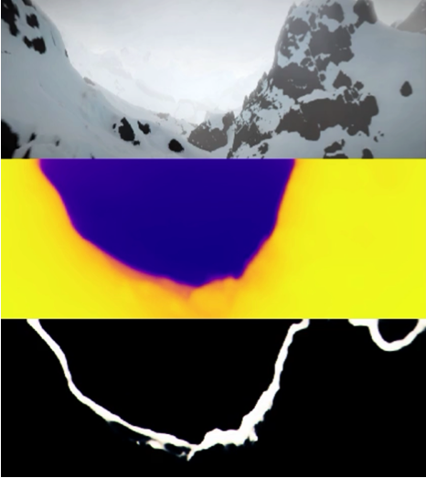
Understanding the 3D structure of a scene can provide important cues for many tasks such as robot navigation [19], motion capture [46], scene understanding [35], and augmented reality [30]. While humans are exceptionally capable of inferring the non-rigid 3D structures from an image, geometric computer vision techniques either require a large amount of labeled data or are capable of learning only from rigid scenes [89]. However, in the real world, scenes often consist of non-rigid and dynamic elements. Thus, it is quite natural to seek for the ability of inferring the depth from an image of any given scene, regardless of whether it is highly dynamic or not. We refer to Fig. 1 for some examples.
The ability of humans to understand their environment geometrically and semantically is mainly acquired through childhood learning. In an attempt to emulate this ability, learning-based strategies have been applied to the problem of depth from single-view. In fact, many learning-based methods already offer very promising progress in this direction. Among them, supervised methods [44, 12, 39] aim to reconstruct the depth of rigid and non-rigid parts during training, whereas many unsupervised methods [24, 89, 88, 26, 13, 49, 78, 47, 48, 27] mainly employ a training strategy which aims to reconstruct the rigid parts of a scene. Although a recent unsupervised method [43] also reconstructs objects translating on a ground plane, it has limitations in terms of modelling highly non-rigid scenes. Other unsupervised methods for non-rigid reconstruction exploit object-specific priors [63, 82, 85], or reconstruct sparse [53] or dense [69, 71] points of a single non-rigid object. Such methods, however, do not have the same applicability or motivation as that of single view scene depth estimation. Unlike the monocular setup, the calibrated stereo (or multi-camera) methods for learning single view depth [25, 52] do not suffer from ambiguities due to non-rigidity and can handle complete scene depth. However, they have significant limitations, particularly when acquiring training data via calibrated stereo pairs is not feasible.
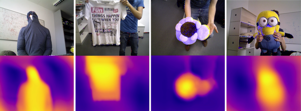
In this work, we are interested in learning to predict dense depth from a single image using an unsupervised monocular pipeline. More importantly, we would like to reconstruct the depth of all parts of the scene during the training, irrespective of the rigidity/non-rigidity of these parts. Our unsupervised setup assumes that only calibrated monocular videos 111Our method can potentially also be used for multi-view setups. with known intrinsics are available during training. Such an assumption is realistic as well as crucial for a wide variety of setups, ranging from consumer to surgical cameras, where depth or stereo acquisition for supervision is often impractical. In this context, learning depth from monocular videos of non-rigid scenes remains an unresolved problem. This is no surprise, given the challenges, e.g., ill-posedness, ambiguities, inconsistent priors.
The success of the unsupervised depth learning methods for rigid scenes can be primarily attributed to the advancements in deep learning and the rigid reconstruction constraints used in such methods. This motivates us to explore the non-rigid 3D reconstruction literature employing various assumptions. Our goal is to keep in mind an overview of the literature and to use the gained insights to build our unsupervised monocular pipeline for depth reconstruction in non-rigid scenes. Our main contributions are threefold:
-
•
We reformulate the Non-Rigid Structure-from-Motion (NRSfM) priors in a novel unified framework using the Euclidean distance matrix measures across views. This contribution is summarized in Table 4.2.
-
•
The utility of the proposed framework is also demonstrated for unsupervised non-rigid monocular depth, by exploiting the as-rigid-as possible (ARAP) prior during CNN training. For the implementation of the ARAP prior, we define and employ a concept of motion embeddings. This contribution is illustrated in Fig. 3.
-
•
Through experiments, we provide interesting new insights towards learning non-rigid scene depths in an unsupervised manner, detailed in our discussion section.
2 Non-Rigid Reconstruction Revisited
Since generic non-rigid 3D reconstruction from a monocular camera is an ill-posed problem, methods in the literature rely on some priors or assumptions about the scene. The most common scene priors can be broadly divided into the following four categories.
Low-Rank (LR). The low-rank prior assumes that non-rigid 3D structures can be expressed as a linear combination of finite basis shapes. The landmark work of Costeira & Kanade [16] developed for orthographic cameras (or slight variations) uses the LR prior for multi-body 3D scene reconstruction. Since, it been widely used in various cases for the 3D reconstruction of single [10, 9, 8, 54, 17, 22, 34, 75, 2, 53, 37] and multiple [84, 3] non-rigid objects.
Scene Motion (SM). Several notable works of Shashua et al. [67, 7, 81, 77] have shown that the known planar/linear motion prior can be exploited to reconstruct the 3D structure of dynamic scenes222The recent work [43] can be seen as an adaptation of [7].. Work of Ozden et al. [55] also tackled dynamic scene 3D reconstruction using the principle of non-accidentalness. An insightful work of Hartley and Vidal [28] reveals that the method of [81] can be indeed extended to the generic non-rigid case, using the low-rank structure and without an explicit motion prior, with only one severe ambiguity, which stems from the fact that the recovered camera motion is relative to the moving points. This in turn implies the unfavorable news that the low-rank prior alone is not sufficient to recover scale-consistent non-rigid 3D structures from monocular projective cameras, when the objects are independently moving in the multi-body setting.
Isometric Deformation (ID). To avoid the algebraic prior of LR, Salzmann et al. [65] and Perriollat et al. [61] introduced the geometric ‘ID’ prior of an object deforming isometrically, which makes non-rigid surface reconstruction possible when used with a known template. Since, the ID prior of the object has been used in many other works [68, 76, 14, 57, 15, 79, 62, 42]. Taylor et al. [73] introduced local-rigidity for non-rigid reconstruction, which is a form of the ID prior. Other related geometric priors have also been exploited in the literature [50, 64, 1]. When objects undergo severe deformations, relying on a geometric prior for the objects and avoiding any explicit camera motion estimation have demonstrated state-of-the art results for non-rigid object reconstruction [59, 56, 62, 23, 51]. The benefit of not estimating the camera motion explicitly can be understood quite intuitively, as the estimated rigid camera motion is merely a motion with respect to the scene. Interested readers may recall the relevant work in [28]. In this regard, the works of Li [42], Ji et al. [33] and Chhatkuli et al. [15] stand out. While reconstructing inextensible structures, [15] formulates an explicit-motion-free problem, which turns out to be equivalent to the rigid case formulation of [42] in the absence of deformations. In fact, the formulation of [15] is shown to be effective for both rigid and non-rigid scenes. All three works [15, 33, 42] are based on the pairwise distance equality in 3D, while [42] uses the same pairwise sampling as [33].
As-Rigid-As-Possible (ARAP). Non-rigid shape modelling using the ARAP assumption is very prevalent in computer graphics [6, 31, 70]. The ARAP assumption maximizes rigidity while penalising stretching, shearing, and compression. ARAP concept has also been used in many works [58, 38] for monocular non-rigid 3D reconstruction. In particular, two works of Parashar et al. [58] and Kumar et al. [38] are noteworthy. Using the shape template of an object, [58] reconstructs the deformed volumetric 3D under the ARAP assumption. On the other hand, [38] demonstrates the practicality of ARAP in depth densification and refinement for non-rigid scenes, using multi-view setups. More interestingly to us, the ARAP prior is sufficient to resolve the scale ambiguity between freely moving parts, i.e. the issue previously discussed by Hartley & Vidal in [28].
In summary, the computation of camera motion becomes ambiguous in complex non-rigid scenes for a monocular camera. Nevertheless, the structure of both rigid scenes and non-rigid objects333Given that the assumed object’s prior is sufficient. can still be recovered without any explicit camera motion estimation. On the other hand, the scale consistent reconstruction intrinsically requires some additional prior, such as the ARAP assumption used in this work.
3 Preliminaries
Notations. We denote matrices with uppercase and their elements with double-indexed lowercase letters: . Similarly, we write vectors and index them as: . The inequality refers to , unless mentioned otherwise. We use special uppercase Latin or Greek letters for sets and graphs, such as and . The lowercase Latin letters, as in , are used for scalars. The set of neighbours of within a radius is given by .
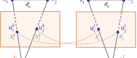
Non-rigid Structure-from-Motion (NRSfM). Our problem formulation is camera motion independent, similar444Similar also in mathematical terms. to [42, 65, 15]. We pose the NRSfM problem as finding point-wise depth in each view. We use superscript to denote the -th image (among ) and subscript to denote the -th point (among ). As illustrated in Fig. 2, we represent the unknown depth as and the known homogeneous image coordinates as . The set of points in the -th view is given as . The Euclidean distance between point and point is denoted as . In our formulation, we use the Euclidean distance matrix:
Definition 3.1 (Euclidean distance matrix)
Euclidean Distance Matrix (EDM), say , is a matrix representing the spacing of points in -dimensional Euclidean space, say , and the entries of are given by, .
Let , be the sought depth of the -th view. We represent the 3D structure in the form, . Let us define the Gram matrix . The EDM for the -th view is then given by:
| (1) |
NRSfM aims to estimate by imposing priors on . For clarity, we present an example of the rigid case.
Example 3.2 (The rigid structure prior)
For noise- and outlier-free rigid scenes, the estimated must satisfy, for all . Intuitively, the distance between any pair of points must be preserved across views. Method of [42] is a variant of this example.
The prior of the above example is also referred as the global rigidity constraint [80, 21]. Weaker than the global rigidity is local rigidity. Interested readers can find a thorough study of local/global rigidity in [42]. Here, we are interested in the non-rigid isometric deformation prior [61, 73, 65, 15]. Let us introduce a weight matrix , whose entries are if for some radius , and otherwise. Then the relaxed isometric prior of [65, 15, 62] aims to reconstruct the depth by solving,
| (2) | ||||
where represents the Hadamard-product. Intuitively, (2) aims to preserve the local Euclidean distances across views. The constraints ensure positive depths in all views. It is important to note that for sufficiently large radii the problem of (2) is equivalent to that of the Example 3.2.
4 This Work
One may use the formulation in Eq. (2) to learn to reconstruct both rigid scenes or non-rigid objects, for known 555For example, [15] uses 2D neighbors to construct .. We however, are interested in reconstructing complex scenes consisting of both, which requires additional priors (recall Section 2). Moreover, it is unclear how to obtain the weight matrix in general cases. We use the ARAP assumption to address the scale ambiguity problem. In this process, the weight matrix is also learned along with the depth. If one aims to exploit other non-rigid priors, later in Section 4.2 we provide a thorough analysis in that direction.
4.1 Problem Formulation
We aim to estimate the depth for each view, and the weight matrix for given view-pairs. Our weights can be interpreted as rigidity scores, between points and . Since, the concept of rigidity is meaningful only for two (or more) views, our rigidity scores are computed accordingly. We consider two points to be rigidly connected, if their distance does not change across views. If one seeks for pair-wise rigidity on generic graphs, several interpretations can be derived based on the graph connectivity [80, 21, 42]. In the context of this paper, we formulate the ARAP assumption as follows:
Definition 4.1 (As-rigid-as-possible)
For a point set under deformation, the as-rigid-as-possible model assumes that every pair-wise distance of the fully connected graph between points, respects at least some degree of rigidity.
We can now formalize our problem statement as follows.
| (3) | ||||
Here, the positive scalars and are the rigidity threshold and the rigidity adjusted maximum allowed distance error, respectively. Very often the point pairs from non-rigid objects respect rigidity. This is when many priors are best justified. In general, local rigidity does not imply global rigidity. For large fully connected graphs though, pair-wise rigidity means global rigidity. We relax this constraint by allowing different edges to have different rigidity scores. We like to draw the reader’s attention on two key (and somewhat related) aspects of our formulation: (1) image pair-wise rigidity scores; and (2) global connectivity.
Our motivation for using individual stems from the following observation: across all frame pairs, most of the edges respect rigidity at least once in the global sense (e.g. stopping objects or periodic motions). This global rigidity can be captured and propagated in the rest of the reconstruction for scale consistency, if the global connectivity is established using the fully connected graph. For local reconstruction, we can rely on local connectivity which often better respects rigidity. Note that the maximum allowed adjusted distance error, i.e. , is measured in the normalized (by the weight matrix) form. This encourages rigid edges to bear higher weights, and vice versa. Such distribution of weights prioritizes the pairs holding rigidity to reconstruct rigidly. On the other hand, non-rigid pairs – if reconstructed correctly at their rigid instant (with highest weight) – can still satisfy the imposed constraints, as long as the extended distance error does not exceed .
4.2 Relation to Previous Works
| Method |
Unsup.-Monoc. |
Non-Rigid |
Rigid prior |
ARAP |
Isom. deform. |
Scene motion |
Low rank |
Constraints | |
| Li [42] | ✓ | ||||||||
| \hdashline Parashar et al. missing [58] | ✓ | ✓ | |||||||
| Kumar et al. missing [38] | ✓ | ✓ | ✓ | ||||||
| \hdashline Salzmann & Fua [65] | ✓ | ✓ | , if , , otherwise | ||||||
| Taylor et al. missing [73] | ✓ | ✓ | ✓ | ||||||
| Chhatkuli et al. missing [15] | ✓ | ✓ | |||||||
| Probst et al. missing [62] | ✓ | ✓ | |||||||
| \hdashline Shashua & Wolf [67] | ✓ | ✓ | ✓ | , if , , otherwise | |||||
| Avidan & Shashua [7] | ✓ | ✓ | |||||||
| Vogel et al. missing [77] | ✓ | ✓ | |||||||
| Li et al. missing [43] | ✓ | ✓ | ✓ | ✓ | |||||
| \hdashline Costeira et al. missing [16] | ✓ | ✓ | , , | ||||||
| Wolf & Shashua [81] | * | ✓ | |||||||
| Hartley & Vidal [28] | * | ✓ | |||||||
| Agudo et al. missing [2] | * | ✓ | |||||||
| \hdashline Wu et al. missing [82] | ✓ | ✓ | |||||||
| \hdashline Ours | ✓ | ✓ | ✓ | ✓ | ✓ | ✓ | ✓ | ||
Heretofore, we have discussed the relationship of our formulation in Eq. (3) to rigidity, ID, and ARAP priors.
Now, we further explore the same with respect to LR and SM, for the completeness of our theoretical framework.
To do so, let us denote and its stacked version .
Our investigation leads to the following relationships between the formulation used in this paper and the prior of the low-rank purely on structures, without explicit camera motion.
Proposition 4.2 (EDM of Low-rank structures)
For 3D structures that can be represented using linear basis, the constraints for all and are necessary
to recover the low-rank structures, using Euclidean distance matrices.
-
Proof
The proof is provided in the suppl. material.

SM prior can also be integrated in our formulation by enforcing rigidity scores. For example, rigid objects with linear constant velocity maintain highest rigidity with respect to parallel lines/planes666Which can be represented using a set of points on them. along the velocity direction. In fact, the exact rigidity scores to the other points can be derived, if the velocity is also known. This is particularly interesting, if the motion prior and image semantics are known, e.g. a rigid car driving on the rigid road with stops, or a rigid surgical tool poking an isometric organ surface. We represent a set of edges whose rigidity scores can be measured (or bounded) in some or all image pairs, as . These scores then can also be used (if necessary with bounds) in our formulation. Needless to say, the SM prior can be used in conjunction with LR in practice [81, 28]. An overview of commonly used priors as discussed in Section 2 in relation to previous works is given in Table 4.2, and presented in a unified framework. Our method can be used for all priors unified in Table 4.2. However, different priors are useful depending on the scene.
Having provided this unified theoretical framework, we proceed with the experimental analysis of our proposed methodology. In this work, we are interested in reconstructing the depth of all parts of a scene, and in that direction we choose to focus on the ARAP prior which is sufficient to resolve the scale ambiguity between freely moving parts, in contrast to priors such as the LR in multi-body settings. That being said, the other priors we unify in Table 4.2 can also be used within our framework to reconstruct scenes/objects operating under different priors, by computing rigidity scores with respect to the corresponding prior and using these scores in our formulation.
5 Learning Depth Using ARAP
We first use problem (3) to learn depth reconstruction from image data, given the dense correspondences between views and . We will then formalize our learning objective for a given image pair and of views and . Our optimization objective can be extended to multi-view images of the same scene. An overview of our learning pipeline is shown in Fig. 3.
Objective and overview. Using a deep convolutional neural network parameterized by , we wish to estimate the depth for a given RGB image of size , as the output of the network.
In order to train the depth network, we use the ARAP prior. For that purpose, we predict depths for the views and as: and , respectively. In order to use the ARAP objective (3), we establish correspondences between views and with a pre-trained optical flow network , whose weights are frozen. We use the dense correspondences for the view pair obtained from to compute the difference of EDMs given by . Next we describe how we obtain the rigidity scores for the view pair .
Motion embeddings. Revisiting the initial optimization problem given in (3), we aim to estimate the weight matrix , whose entries represent the rigidity between points , across the transformation between the views . To derive this weight matrix , we propose to learn per-pixel motion embeddings, whose similarity indicates the sought rigidity between points. In particular, we seek for a dense and complete map of motion embeddings, given a pair of views . To this end, we make use of another neural network, parameterized by , to learn the motion embeddings:
Definition 5.1 (Motion embedding matrix)
A motion embedding matrix, say , is a matrix representing points in -dimensional Euclidean space, in which . The entry represents a motion embedding vector for each point in the -th view, representing the motion that the point undergoes across the given view pair .
Having obtained the motion embedding matrix , we derive the entries of from the pairwise distances between the motion embedding vectors and . It should be noted that we expect a higher weight when the distance between the motion embedding vectors are smaller, and vice versa. With this consideration, we formulate the motion similarity scores for every pair (as illustrated in Fig. 4) as,
| (4) |
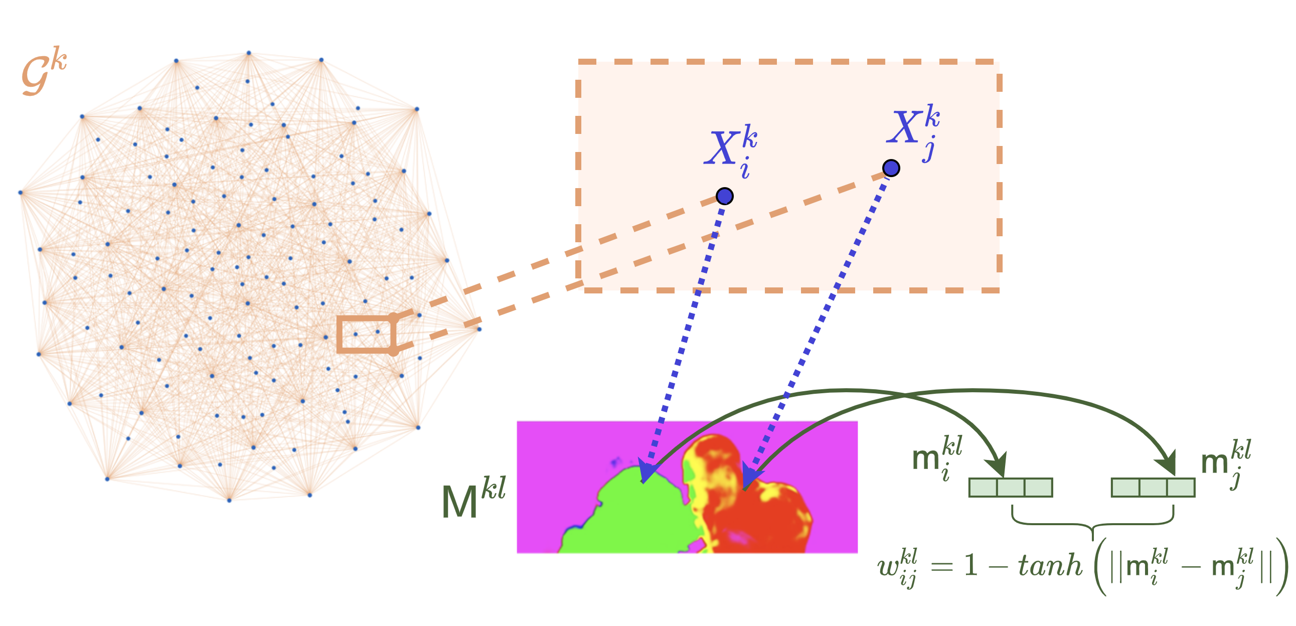
Edge Sampling. We aim to compute the motion similarity scores, , ideally for all possible point pair combinations. However, performing this computation is not tractable considering the number of pixels. Therefore, from the graph for the -th view, say , we uniformly sample a random subset of all edges (point pairs) for the loss computation. The sampled edges are denoted as . Using this subset , we compute a weight matrix , whose entries are given by
| (5) |
Loss Formulation. Using (4) and (5), we reformulate the problem of (3) as a loss function to train our networks, parameterized by , as follows:
| (6) |
The normalization factor is introduced for numerical stability and to avoid reconstructions with near-zero depth values. The constraints of (3) are imposed in the network output: Depths are ensured to be positive by using a sigmoid on inverse depth output from the network. Similarly, the weights are bounded by using (6), followed by a -offset and clamping of the weight values to in progression (to enforce the constraints of (3)). Computation of (6) can be efficiently performed by exploiting the sparsity of . During the calculation, we only iterate through the indices with non-zero entries of . We additionally incorporated a weight-norm regularization term in our training objective, i.e. , to control the maximization of the weights. Further implementation details can be found in the supplementary. We summarize our loss computation process in Algorithm 1.
Network structure. Our depth network consists of a ResNet-18 based encoder and a decoder. The input to our depth network is a single RGB image, and the output from the network is a single depth map of the same size. Our per-pixel motion embedding network also consists of a multi-input ResNet-18 based encoder and a decoder. The input to the motion embedding network is a pair of images, whose channels are concatenated to create a single input tensor before being passed through the network. The output from the motion embedding network is a motion-embedding map, which, in our case, has 3 channels.
Loss computation between two views for ARAP prior.
6 Experimental Results
We perform a variety of experiments to demonstrate the performance of our unsupervised monocular pipeline for non-rigid scenes. In addition to assessing the depth reconstruction performance, we also evaluate the learned motion embeddings in terms of the motion segmentation task.
| VolumeDeform [32] dataset | MPI Sintel [11] dataset | ||||||||||||||
| Scene | Method | \cellcolorred!25Abs Rel | \cellcolorred!25Sq Rel | \cellcolorred!25RMSE | \cellcolorred!25RMSE | \cellcolorblue!25 | \cellcolorblue!25 | \cellcolorblue!25 | \cellcolorred!25Abs Rel | \cellcolorred!25Sq Rel | \cellcolorred!25RMSE | \cellcolorred!25RMSE | \cellcolorblue!25 | \cellcolorblue!25 | \cellcolorblue!25 |
| Mostly | PackNet [27] | 0.691 | 2.879 | 10.544 | 1.739 | 0.425 | 0.591 | 0.667 | 0.355 | 9.278 | 10.923 | 0.544 | 0.499 | 0.789 | 0.885 |
| Rigid | Li et al. [43] | 0.871 | 5.267 | 4.284 | 0.757 | 0.214 | 0.496 | 0.680 | 0.412 | 3.798 | 3.256 | 0.663 | 0.476 | 0.676 | 0.817 |
| Seq. | Ours w/ motion | 0.562 | 2.483 | 5.327 | 0.700 | 0.294 | 0.523 | 0.688 | 0.213 | 1.400 | 6.724 | 0.533 | 0.566 | 0.807 | 0.886 |
| Ours w/o motion | 0.549 | 2.441 | 5.315 | 0.694 | 0.300 | 0.525 | 0.704 | 0.255 | 1.710 | 3.780 | 0.528 | 0.493 | 0.794 | 0.883 | |
| Non- | PackNet [27] | 0.774 | 3.595 | 4.196 | 2.680 | 0.242 | 0.386 | 0.535 | 1.480 | 14.737 | 7.465 | 0.882 | 0.327 | 0.508 | 0.640 |
| Rigid | Li et al. [43] | 1.217 | 9.254 | 4.391 | 0.852 | 0.211 | 0.419 | 0.594 | 1.312 | 15.242 | 6.278 | 0.895 | 0.320 | 0.498 | 0.618 |
| Seq. | Ours w/ motion | 0.562 | 1.675 | 2.576 | 0.533 | 0.492 | 0.673 | 0.823 | 0.638 | 4.833 | 7.602 | 0.833 | 0.442 | 0.615 | 0.713 |
| Ours w/o motion | 0.519 | 1.363 | 2.767 | 0.553 | 0.373 | 0.635 | 0.817 | 0.617 | 4.686 | 7.681 | 0.835 | 0.406 | 0.594 | 0.708 | |
| All | PackNet [27] | 0.673 | 3.623 | 6.585 | 2.227 | 0.299 | 0.465 | 0.576 | 1.134 | 13.057 | 8.529 | 0.778 | 0.380 | 0.594 | 0.716 |
| Seq. | Li et al. [43] | 0.992 | 6.855 | 4.268 | 0.777 | 0.211 | 0.465 | 0.652 | 1.012 | 11.427 | 5.271 | 0.818 | 0.372 | 0.557 | 0.684 |
| Ours w/ motion | 0.578 | 2.513 | 5.210 | 0.726 | 0.400 | 0.597 | 0.748 | 0.507 | 3.777 | 7.332 | 0.741 | 0.480 | 0.674 | 0.766 | |
| Ours w/o motion | 0.540 | 2.301 | 4.294 | 0.721 | 0.349 | 0.582 | 0.753 | 0.505 | 3.770 | 6.481 | 0.741 | 0.433 | 0.655 | 0.762 | |
Datasets. In our experiments, we use MPI Sintel [11], VolumeDeform [32], and Hamlyn Laparascopic Video Dataset [87]. From the MPI Sintel training subset, we select a set of 14 final-pass sequences with varying levels of motions. We also use the VolumeDeform dataset consisting of 8 sequences for further experiments on deforming scenes. Lastly, we evaluate our method on the Hamlyn Centre Laparoscopic Video Dataset, which consists of rectified stereo image pairs collected from a partial nephrectomy. Ground-truth depth maps for VolumeDeform are obtained from the provided depth recordings; and OpenSFM [5, 4] was used to obtain ground-truth depth for Hamlyn using the calibrated stereo pairs in the dataset. For Sintel, both ground-truth depth maps as well as optical flow maps are provided, which is not the case for the other two datasets. A pre-trained supervised optical flow network, RAFT [74], performs reasonably well on VolumeDeform for estimating dense correspondences. On Hamlyn, due to a large domain gap, we fine-tune an unsupervised model, DDFlow [45].
| Motion Depth Image | 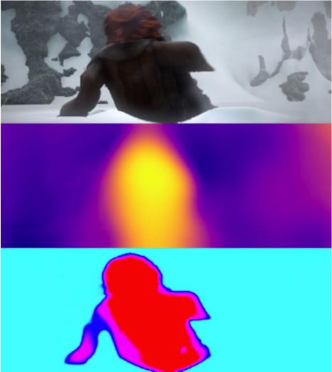 |
 |
 |
| Motion Depth Image | 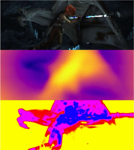 |
 |
 |
| Motion Depth Image | 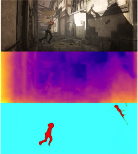 |
 |
 |
Training Details. We follow two different sets of experiments: test-time training or inference. As the small volumes of MPI Sintel and VolumeDeform datasets do not yet enable us to train a depth network that can generalize, we perform test-time training for each image sequence, i.e. we train separate models for each sequence, for our methods and the deep baselines. In this pipeline, for all of the methods, the training is rather used as an optimization procedure for solving for the depth in all frames, given an image sequence. For the Hamlyn dataset where the amount of data enables us to train models that could generalize, we present inference results. We use the original training and test split from the Hamlyn dataset, and further create train/val/test splits. We implemented our model in PyTorch [60]. In all experiments, the ResNet18-based depth encoder and motion-embedding encoder were initialized with weights from ImageNet [18] pre-training. Adam [36] optimizer with , was used, in combination with a learning rate decay by 0.1 every 10 epochs. We follow a two-stage training. In the first stage, we jointly train the motion-embedding network and the depth network. In the second stage, we freeze the weights of the motion-embedding network, and re-initialize the depth network training. In the latter stage, we apply a -offset to the weights, to impose the constraint from (3). For the selection of the edges, we uniformly sample pairs of points with correspondences in the consecutive frame. We empirically find 100K pairs (edges) to provide a suitable trade-off between increased memory requirements and slow convergence. Further details are in the supplementary material.
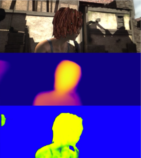
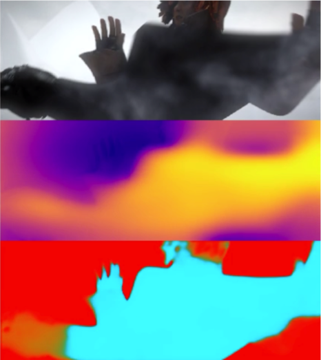
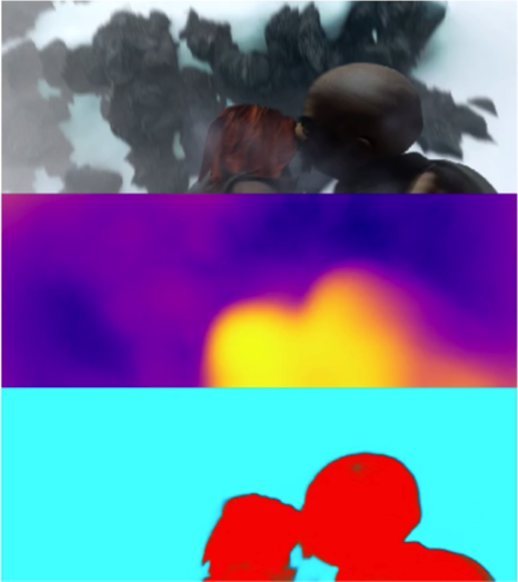
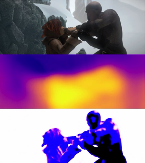
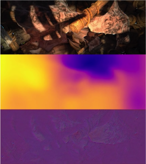
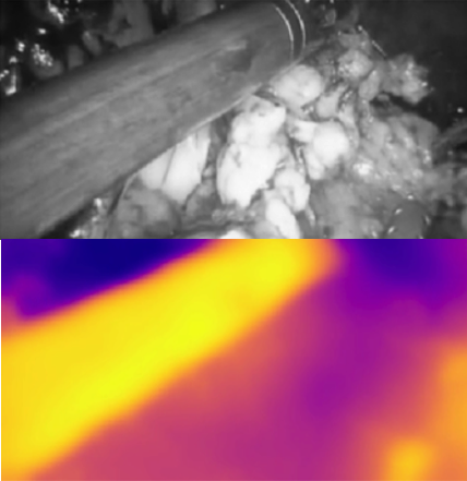
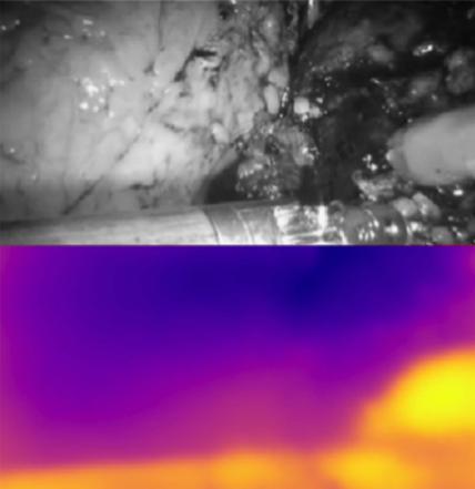
Depth reconstruction results. Our qualitative results are demonstrated in Fig. 1, 5 and 6. We report our results by performing per-image median ground-truth scaling for each method, as introduced in [89]. For the MPI Sintel dataset, we evaluate the performance only where the GT depth is smaller than 50 m. For the other datasets, we evaluate the depth for every point where the GT is available. As shown in Table 2, 3 and 4, we report results from “Ours w/ motion”, and “Ours w/o motion”. “Ours w/ motion” refers to the setting we described in Section 5, where we learn the motion similarity scores serving the ARAP prior. “Ours w/o motion” refers to the same unsupervised pipeline, except that all rigidity scores are explicitly set to 1. With this modification, piecewise-rigidity is implied during training. In Table 3, we further compare the performance of our methods, by separately evaluating the performance in dynamic and static parts of the images. In Table 4, the results from the non-rigid reconstruction models DLH [17], MDH [62] and MaxRig [33] were obtained using the complete test sequence to perform reconstruction. The evaluations for DLH and MaxRig were performed only at the reconstructed points as these methods provide sparse reconstructions.
| \cellcolorred!25Abs | \cellcolorred!25Sq | \cellcolorred!25RMSE | \cellcolorred!25RMSE | \cellcolorblue!25 | \cellcolorblue!25 | \cellcolorblue!25 | ||
| Scene | Method | \cellcolorred!25Rel | \cellcolorred!25Rel | \cellcolorred!25 | \cellcolorred!25 | \cellcolorblue!25 | \cellcolorblue!25 | \cellcolorblue!25 |
| Rigid | w/ motion | 0.387 | 2.276 | 5.954 | 0.778 | 0.407 | 0.632 | 0.718 |
| Parts | w/o motion | 0.393 | 2.335 | 5.529 | 0.787 | 0.431 | 0.636 | 0.725 |
| Non-Rig | w/ motion | 0.702 | 1.828 | 1.618 | 0.503 | 0.348 | 0.608 | 0.795 |
| Parts | w/o motion | 0.889 | 5.879 | 8.919 | 0.551 | 0.329 | 0.592 | 0.732 |
| Depth Image | 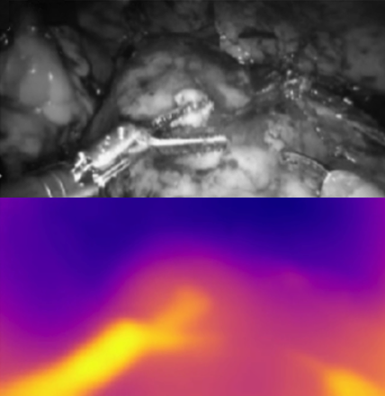 |
 |
 |
| \cellcolorred!25Abs | \cellcolorred!25Sq | \cellcolorred!25RMSE | \cellcolorred!25RMSE | \cellcolorblue!25 | \cellcolorblue!25 | \cellcolorblue!25 | |
| Method | \cellcolorred!25Rel | \cellcolorred!25Rel | \cellcolorred!25 | \cellcolorred!25 | \cellcolorblue!25 | \cellcolorblue!25 | \cellcolorblue!25 |
| PackNet [27] | 0.389 | 2.533 | 4.378 | 0.418 | 0.469 | 0.733 | 0.882 |
| Li et al. [43] | 0.344 | 2.078 | 4.169 | 0.385 | 0.484 | 0.772 | 0.907 |
| DLH [17] | 0.644 | 5.150 | 6.108 | 0.611 | 0.291 | 0.547 | 0.744 |
| MDH [62] | 1.222 | 14.210 | 4.530 | 0.412 | 0.572 | 0.829 | 0.945 |
| MaxRig [33] | 0.232 | 1.083 | 3.247 | 0.294 | 0.587 | 0.850 | 0.962 |
| N-NRSfM [69] | 0.392 | 2.548 | 5.295 | 0.730 | 0.361 | 0.626 | 0.779 |
| Ours w/ motion | 0.217 | 0.941 | 3.120 | 0.279 | 0.608 | 0.886 | 0.977 |
| Ours w/o motion | 0.213 | 0.921 | 3.065 | 0.272 | 0.618 | 0.891 | 0.980 |
Motion segmentation results. We also evaluate the performance of our per-pixel motion embedding. As the ground-truth motion-embeddings are not available, we perform the evaluation on MPI Sintel dataset using the available ground-truth motion segmentation maps [83]. With that purpose, we first calculate the static background embedding vector by taking channel-wise median of the image border embeddings, assuming the image border mostly consists of the static background. Then we separate the static part from the dynamic parts of the scene, by thresholding the distances between the static background embedding and each per-pixel motion embedding vectors. In Table 5, we compare the performance of our model with two recent works [72] and [86], and demonstrate our competitive results for the motion segmentation task in Fig. 7.
| Frame | |||
| GT | |||
| [72] | |||
| [86] | |||
| Ours |
Discussion. Through numerous experiments, we demonstrated that our formulation with ARAP assumption performs well, even for highly dynamic scenes. However, for some scenes with small deformations, we have observed that the pairwise rigidity assumption performs better. Such behaviour is often due to the short video sequence-based supervision. Often, the scene rigidity may be maintained for a small duration. More importantly, large scene parts are often rigid, which offer better reconstruction when stronger priors are employed. However, rigid reconstruction can be performed rather easily, and despite the fact that most of the time dynamic and deformable objects are of higher interest, they are also more difficult to reconstruct without a suitable prior. In this direction, we investigated several of the commonly used priors, and demonstrated the utility of ARAP assumption for our pipeline. We believe that our framework can be very useful when the scene-specific priors are known for individual use-cases. Note that our formulation highly differs from existing unsupervised monocular depth methods. More specifically, the sole source of self-supervision in our case is the minimization of the geometric errors, and not the photometric errors. This is particularly beneficial for avoiding reconstruction errors that could stem from photometric errors, especially in the presence of deformations. This fact, along with the motion-independent formulation may explain why our pair-wise rigidity works better than a motion-explicit rigid unsupervised learning method [27] for non-rigid scenes. Even if we seek for pair-wise rigidity in non-rigid scenes, since the exact rigid reconstruction is not feasible, the optimal reconstruction is bound to be ARAP.
7 Conclusion
We demonstrated the possibility for unsupervised learning of depth using monocular videos of non-rigid scenes in order to infer depth from a single image. Unsupervised learning is enabled by established priors used in the NRSfM literature. Building upon existing works, we reformulated commonly used NRSfM priors within a unified framework suitable for neural network training. We further investigated the utility of the ARAP prior for dense depth reconstruction from a single view. Our experiments demonstrate improvements over the alternative methods on numerous datasets. The improvements can be attributed to our geometric error-based loss function (6) computed directly in the 3D reconstruction space. We assumed only the minimum necessary prior in this work, as we aimed to learn without any supervision (including additional scene priors). Depending on scene properties, different priors can be integrated into our pipeline in a similar way, boosting the performance further.
Acknowledgments. This research was partly supported by Innosuisse funding (Grant No. 34475.1 IP-ICT), by FIFA, and by the ETH Zurich project with Specta and EU H2020 ENCORE (Grant No. 820434).
References
- [1] Antonio Agudo, Lourdes Agapito, Begona Calvo, and Jose MM Montiel. Good vibrations: A modal analysis approach for sequential non-rigid structure from motion. In Proceedings of the IEEE Conference on computer vision and pattern recognition, pages 1558–1565, 2014.
- [2] Antonio Agudo, Melcior Pijoan, and Francesc Moreno-Noguer. Image collection pop-up: 3d reconstruction and clustering of rigid and non-rigid categories. In Proceedings of the IEEE conference on computer vision and pattern recognition, pages 2607–2615, 2018.
- [3] Ijaz Akhter, Yaser Sheikh, Sohaib Khan, and Takeo Kanade. Trajectory space: A dual representation for nonrigid structure from motion. IEEE Transactions on Pattern Analysis and Machine Intelligence, 33(7):1442–1456, 2010.
- [4] Pablo Fernández Alcantarilla, Adrien Bartoli, and Andrew J. Davison. Kaze features. In Andrew Fitzgibbon, Svetlana Lazebnik, Pietro Perona, Yoichi Sato, and Cordelia Schmid, editors, Computer Vision – ECCV 2012, pages 214–227, Berlin, Heidelberg, 2012. Springer Berlin Heidelberg.
- [5] Pablo Fernández Alcantarilla, Jesus Nuevo, and Adrien Bartoli. Fast explicit diffusion for accelerated features in nonlinear scale spaces. In BMVC, 2013.
- [6] Marc Alexa, Daniel Cohen-Or, and David Levin. As-rigid-as-possible shape interpolation. In Proceedings of the 27th annual conference on Computer graphics and interactive techniques, pages 157–164, 2000.
- [7] Shai Avidan and Amnon Shashua. Trajectory triangulation: 3d reconstruction of moving points from a monocular image sequence. IEEE Transactions on Pattern Analysis and Machine Intelligence, 22(4):348–357, 2000.
- [8] Adrien Bartoli, Vincent Gay-Bellile, Umberto Castellani, Julien Peyras, Søren Olsen, and Patrick Sayd. Coarse-to-fine low-rank structure-from-motion. In 2008 IEEE Conference on Computer Vision and Pattern Recognition, pages 1–8. IEEE, 2008.
- [9] Matthew Brand and Rahul Bhotika. Flexible flow for 3d nonrigid tracking and shape recovery. In Proceedings of the 2001 IEEE Computer Society Conference on Computer Vision and Pattern Recognition. CVPR 2001, volume 1, pages I–I. IEEE, 2001.
- [10] Christoph Bregler, Aaron Hertzmann, and Henning Biermann. Recovering non-rigid 3d shape from image streams. In Proceedings IEEE Conference on Computer Vision and Pattern Recognition. CVPR 2000 (Cat. No. PR00662), volume 2, pages 690–696. IEEE, 2000.
- [11] Daniel Butler, Jonas Wulff, Garrett Stanley, and Michael Black. A naturalistic open source movie for optical flow evaluation. In A. Fitzgibbon et al. (Eds.), editor, European Conf. on Computer Vision (ECCV), Part IV, LNCS 7577, pages 611–625. Springer-Verlag, Oct. 2012.
- [12] Weifeng Chen, Zhao Fu, Dawei Yang, and Jia Deng. Single-image depth perception in the wild. CoRR, abs/1604.03901, 2016.
- [13] Yuhua Chen, Cordelia Schmid, and Cristian Sminchisescu. Self-supervised learning with geometric constraints in monocular video: Connecting flow, depth, and camera. CoRR, abs/1907.05820, 2019.
- [14] Ajad Chhatkuli, Daniel Pizarro, and Adrien Bartoli. Non-rigid shape-from-motion for isometric surfaces using infinitesimal planarity. In BMVC, 2014.
- [15] Ajad Chhatkuli, Daniel Pizarro, Toby Collins, and Adrien Bartoli. Inextensible non-rigid shape-from-motion by second-order cone programming. In Proceedings of the IEEE Conference on Computer Vision and Pattern Recognition, pages 1719–1727, 2016.
- [16] João Paulo Costeira and Takeo Kanade. A multibody factorization method for independently moving objects. International Journal of Computer Vision, 29(3):159–179, 1998.
- [17] Yuchao Dai, Hongdong Li, and Mingyi He. A simple prior-free method for non-rigid structure-from-motion factorization. In 2012 IEEE Conference on Computer Vision and Pattern Recognition, pages 2018–2025. IEEE, 2012.
- [18] Jia Deng, Wei Dong, Richard Socher, Li-Jia Li, Kai Li, and Fei Fei Li. Imagenet: a large-scale hierarchical image database. In IEEE Conference on Computer Vision and Pattern Recognition, pages 248–255, 06 2009.
- [19] Sotirios Diamantas, Anastasios Oikonomidis, and Richard Crowder. Depth estimation for autonomous robot navigation: A comparative approach. In 2010 IEEE International Conference on Imaging Systems and Techniques, pages 426–430, 2010.
- [20] David Eigen, Christian Puhrsch, and Rob Fergus. Depth map prediction from a single image using a multi-scale deep network. CoRR, abs/1406.2283, 2014.
- [21] Tolga Eren, Peter N Belhumeur, and A Stephen Morse. Closing ranks in vehicle formations based on rigidity. In Proceedings of the 41st IEEE Conference on Decision and Control, 2002., volume 3, pages 2959–2964. IEEE, 2002.
- [22] Katerina Fragkiadaki, Marta Salas, Pablo Arbelaez, and Jitendra Malik. Grouping-based low-rank trajectory completion and 3d reconstruction. In Advances in Neural Information Processing Systems, pages 55–63, 2014.
- [23] Mathias Gallardo, Daniel Pizarro, Toby Collins, and Adrien Bartoli. Shape-from-template with curves. International Journal of Computer Vision, 128(1):121–165, 2020.
- [24] Ravi Garg, Vijay Kumar B. G, and Ian D. Reid. Unsupervised CNN for single view depth estimation: Geometry to the rescue. In ECCV, 2016.
- [25] Clément Godard, Oisin Mac Aodha, and Gabriel J. Brostow. Unsupervised monocular depth estimation with left-right consistency. CoRR, abs/1609.03677, 2016.
- [26] Clément Godard, Oisin Mac Aodha, and Gabriel J. Brostow. Digging into self-supervised monocular depth estimation. CoRR, abs/1806.01260, 2018.
- [27] Vitor Guizilini, Rares Ambrus, Sudeep Pillai, and Adrien Gaidon. Packnet-sfm: 3d packing for self-supervised monocular depth estimation. CoRR, abs/1905.02693, 2019.
- [28] Richard Hartley and René Vidal. Perspective nonrigid shape and motion recovery. In European Conference on Computer Vision, pages 276–289. Springer, 2008.
- [29] Kaiming He, Xiangyu Zhang, Shaoqing Ren, and Jian Sun. Deep residual learning for image recognition. CoRR, abs/1512.03385, 2015.
- [30] Florian Heinrich, Kai Bornemann, Kai Lawonn, and Christian Hansen. Depth perception in projective augmented reality: An evaluation of advanced visualization techniques. In 25th ACM Symposium on Virtual Reality Software and Technology, VRST ’19, New York, NY, USA, 2019. Association for Computing Machinery.
- [31] Takeo Igarashi, Tomer Moscovich, and John F Hughes. As-rigid-as-possible shape manipulation. ACM transactions on Graphics (TOG), 24(3):1134–1141, 2005.
- [32] Matthias Innmann, Michael Zollhöfer, Matthias Nießner, Christian Theobalt, and Marc Stamminger. Volumedeform: Real-time volumetric non-rigid reconstruction. In Bastian Leibe, Jiri Matas, Nicu Sebe, and Max Welling, editors, Computer Vision - ECCV 2016 - 14th European Conference, Amsterdam, The Netherlands, October 11-14, 2016, Proceedings, Part VIII, volume 9912 of Lecture Notes in Computer Science, pages 362–379. Springer, 2016.
- [33] Pan Ji, Hongdong Li, Yuchao Dai, and Ian D. Reid. ”maximizing rigidity” revisited: a convex programming approach for generic 3d shape reconstruction from multiple perspective views. CoRR, abs/1707.05009, 2017.
- [34] Imran Khan. Non-rigid structure-from-motion with uniqueness constraint and low rank matrix fitting factorization. IEEE transactions on multimedia, 16(5):1350–1357, 2014.
- [35] Byung-soo Kim, Pushmeet Kohli, and Silvio Savarese. 3d scene understanding by voxel-crf. In Proceedings of the IEEE International Conference on Computer Vision, pages 1425–1432, 2013.
- [36] Diederik P. Kingma and Jimmy Ba. Adam: A method for stochastic optimization, 2014. cite arxiv:1412.6980 Comment: Published as a conference paper at the 3rd International Conference for Learning Representations, San Diego, 2015.
- [37] Chen Kong and Simon Lucey. Deep non-rigid structure from motion. In Proceedings of the IEEE International Conference on Computer Vision, 2019.
- [38] Suryansh Kumar, Ram Srivatsav Ghorakavi, Yuchao Dai, and Hongdong Li. Dense depth estimation of a complex dynamic scene without explicit 3d motion estimation. arXiv preprint arXiv:1902.03791, 2019.
- [39] Yevhen Kuznietsov, Jörg Stückler, and Bastian Leibe. Semi-supervised deep learning for monocular depth map prediction. CoRR, abs/1702.02706, 2017.
- [40] Lubor Ladicky, Jianbo Shi, and Marc Pollefeys. Pulling things out of perspective. CVPR, 2014.
- [41] Congcong Li, Adarsh Kowdle, Ashutosh Saxena, and Tsuhan Chen. Towards holistic scene understanding: Feedback enabled cascaded classification models. CoRR, abs/1110.5102, 2011.
- [42] Hongdong Li. Multi-view structure computation without explicitly estimating motion. In 2010 IEEE Computer Society Conference on Computer Vision and Pattern Recognition, pages 2777–2784. IEEE, 2010.
- [43] Hanhan Li, Ariel Gordon, Hang Zhao, Vincent Casser, and Anelia Angelova. Unsupervised monocular depth learning in dynamic scenes. arXiv preprint arXiv:2010.16404, 2020.
- [44] Chao Liu, Jinwei Gu, Kihwan Kim, Srinivasa G. Narasimhan, and Jan Kautz. Neural rgb->d sensing: Depth and uncertainty from a video camera. CoRR, abs/1901.02571, 2019.
- [45] Pengpeng Liu, Irwin King, Michael R. Lyu, and Jia Xu. Ddflow: Learning optical flow with unlabeled data distillation. In AAAI, 2019.
- [46] Matthew Loper, Naureen Mahmood, and Michael J. Black. Mosh: Motion and shape capture from sparse markers. ACM Trans. Graph., 33(6), Nov. 2014.
- [47] Chenxu Luo, Zhenheng Yang, Peng Wang, Yang Wang, Wei Xu, Ram Nevatia, and Alan L. Yuille. Every pixel counts ++: Joint learning of geometry and motion with 3d holistic understanding. CoRR, abs/1810.06125, 2018.
- [48] Xuan Luo, Jia-Bin Huang, Richard Szeliski, Kevin Matzen, and Johannes Kopf. Consistent video depth estimation, 2020.
- [49] Reza Mahjourian, Martin Wicke, and Anelia Angelova. Unsupervised learning of depth and ego-motion from monocular video using 3d geometric constraints. CoRR, abs/1802.05522, 2018.
- [50] Abed Malti, Richard Hartley, Adrien Bartoli, and Jae-Hak Kim. Monocular template-based 3d reconstruction of extensible surfaces with local linear elasticity. In Proceedings of the IEEE conference on computer vision and pattern recognition, pages 1522–1529, 2013.
- [51] Abed Malti and Cédric Herzet. Elastic shape-from-template with spatially sparse deforming forces. In Proceedings of the IEEE Conference on Computer Vision and Pattern Recognition, pages 3337–3345, 2017.
- [52] Ishit Mehta, Parikshit Sakurikar, and PJ Narayanan. Structured adversarial training for unsupervised monocular depth estimation. In 2018 International Conference on 3D Vision (3DV), pages 314–323. IEEE, 2018.
- [53] David Novotny, Nikhila Ravi, Benjamin Graham, Natalia Neverova, and Andrea Vedaldi. C3dpo: Canonical 3d pose networks for non-rigid structure from motion. In Proceedings of the IEEE International Conference on Computer Vision, 2019.
- [54] Carl Olsson and Magnus Oskarsson. A convex approach to low rank matrix approximation with missing data. In Scandinavian Conference on Image Analysis, pages 301–309. Springer, 2009.
- [55] K. Ozden, K. Cornelis, L. Van Eycken, and L. Van Gool. Reconstructing 3d independent motions using non-accidentalness. In CVPR, volume 1, pages I–819–I–825 Vol.1, 2004.
- [56] Shaifali Parashar, Adrien Bartoli, and Daniel Pizarro. Robust isometric non-rigid structure-from-motion. arXiv preprint arXiv:2010.04690, 2020.
- [57] Shaifali Parashar, Daniel Pizarro, and Adrien Bartoli. Isometric non-rigid shape-from-motion in linear time. In Proceedings of the IEEE Conference on Computer Vision and Pattern Recognition, pages 4679–4687, 2016.
- [58] Shaifali Parashar, Daniel Pizarro, Adrien Bartoli, and Toby Collins. As-rigid-as-possible volumetric shape-from-template. In Proceedings of the IEEE International Conference on Computer Vision, pages 891–899, 2015.
- [59] Shaifali Parashar, Mathieu Salzmann, and Pascal Fua. Local non-rigid structure-from-motion from diffeomorphic mappings. In Proceedings of the IEEE/CVF Conference on Computer Vision and Pattern Recognition, pages 2059–2067, 2020.
- [60] Adam Paszke, Sam Gross, Francisco Massa, Adam Lerer, James Bradbury, Gregory Chanan, Trevor Killeen, Zeming Lin, Natalia Gimelshein, Luca Antiga, Alban Desmaison, Andreas Kopf, Edward Yang, Zachary DeVito, Martin Raison, Alykhan Tejani, Sasank Chilamkurthy, Benoit Steiner, Lu Fang, Junjie Bai, and Soumith Chintala. Pytorch: An imperative style, high-performance deep learning library. In H. Wallach, H. Larochelle, A. Beygelzimer, F. d'Alché-Buc, E. Fox, and R. Garnett, editors, Advances in Neural Information Processing Systems 32, pages 8024–8035. Curran Associates, Inc., 2019.
- [61] Mathieu Perriollat, Richard Hartley, and Adrien Bartoli. Monocular template-based reconstruction of inextensible surfaces. International journal of computer vision, 95(2):124–137, 2011.
- [62] Thomas Probst, Danda Pani Paudel, Ajad Chhatkuli, and Luc Van Gool. Incremental non-rigid structure-from-motion with unknown focal length. In Proceedings of the European Conference on Computer Vision (ECCV), pages 756–771, 2018.
- [63] Anurag Ranjan, Timo Bolkart, Soubhik Sanyal, and Michael J. Black. Generating 3d faces using convolutional mesh autoencoders. In Proceedings of the European Conference on Computer Vision (ECCV), pages 704–720, 2018.
- [64] Chris Russell, Rui Yu, and Lourdes Agapito. Video pop-up: Monocular 3d reconstruction of dynamic scenes. In European conference on computer vision, pages 583–598. Springer, 2014.
- [65] Mathieu Salzmann and Pascal Fua. Linear local models for monocular reconstruction of deformable surfaces. IEEE Transactions on Pattern Analysis and Machine Intelligence, 33(5):931–944, 2010.
- [66] A. Saxena, M. Sun, and A. Y. Ng. Make3d: Learning 3d scene structure from a single still image. IEEE Transactions on Pattern Analysis and Machine Intelligence, 31(5):824–840, May 2009.
- [67] Amnon Shashua and Lior Wolf. Homography tensors: On algebraic entities that represent three views of static or moving planar points. In European Conference on Computer Vision, pages 507–521. Springer, 2000.
- [68] Shuhan Shen, Wenhuan Shi, and Yuncai Liu. Monocular 3-d tracking of inextensible deformable surfaces under -norm. IEEE Transactions on Image Processing, 19(2):512–521, 2009.
- [69] Vikramjit Sidhu, Edgar Tretschk, Vladislav Golyanik, Antonio Agudo, and Christian Theobalt. Neural dense non-rigid structure from motion with latent space constraints. In European Conference on Computer Vision (ECCV), 2020.
- [70] Olga Sorkine and Marc Alexa. As-rigid-as-possible surface modeling. In Symposium on Geometry processing, volume 4, pages 109–116, 2007.
- [71] Srinath Sridhar, Davis Rempe, Julien Valentin, Bouaziz Sofien, and Leonidas J Guibas. Multiview aggregation for learning category-specific shape reconstruction. In Advances in Neural Information Processing Systems, volume 32, 2019.
- [72] Tatsunori Taniai, Sudipta N. Sinha, and Yoichi Sato. Fast multi-frame stereo scene flow with motion segmentation. CoRR, abs/1707.01307, 2017.
- [73] Jonathan Taylor, Allan Jepson, and Kiriakos Kutulakos. Non-rigid structure from locally-rigid motion. In Proceedings of the IEEE Computer Society Conference on Computer Vision and Pattern Recognition, 2010.
- [74] Zachary Teed and Jia Deng. RAFT: recurrent all-pairs field transforms for optical flow. In Andrea Vedaldi, Horst Bischof, Thomas Brox, and Jan-Michael Frahm, editors, Computer Vision - ECCV 2020 - 16th European Conference, Glasgow, UK, August 23-28, 2020, Proceedings, Part II, volume 12347 of Lecture Notes in Computer Science, pages 402–419. Springer, 2020.
- [75] Jack Valmadre, Sridha Sridharan, Simon Denman, Clinton Fookes, and Simon Lucey. Closed-form solutions for low-rank non-rigid reconstruction. In 2015 International Conference on Digital Image Computing: Techniques and Applications (DICTA), pages 1–6. IEEE, 2015.
- [76] Sara Vicente and Lourdes Agapito. Soft inextensibility constraints for template-free non-rigid reconstruction. In European conference on computer vision, pages 426–440. Springer, 2012.
- [77] Christoph Vogel, Konrad Schindler, and Stefan Roth. 3d scene flow estimation with a piecewise rigid scene model. International Journal of Computer Vision, 115(1):1–28, 2015.
- [78] Chaoyang Wang, José Miguel Buenaposada, Rui Zhu, and Simon Lucey. Learning depth from monocular videos using direct methods. CoRR, abs/1712.00175, 2017.
- [79] Xuan Wang, Mathieu Salzmann, Fei Wang, and Jizhong Zhao. Template-free 3d reconstruction of poorly-textured nonrigid surfaces. In European Conference on Computer Vision, pages 648–663. Springer, 2016.
- [80] Walter Whiteley. Rigidity and scene analysis, 2004.
- [81] Lior Wolf and Amnon Shashua. On projection matrices pk to p2, k= 3,…, 6, and their applications in computer vision. International Journal of Computer Vision, 48(1):53–67, 2002.
- [82] Shangzhe Wu, Christian Rupprecht, and Andrea Vedaldi. Unsupervised learning of probably symmetric deformable 3d objects from images in the wild. In Proceedings of the IEEE/CVF Conference on Computer Vision and Pattern Recognition, pages 1–10, 2020.
- [83] Jonas Wulff, Laura Sevilla-Lara, and Michael J. Black. Optical flow in mostly rigid scenes. In Proceedings IEEE Conference on Computer Vision and Pattern Recognition (CVPR) 2017, pages 6911–6920, Piscataway, NJ, USA, July 2017. IEEE.
- [84] Jing Xiao and Takeo Kanade. Uncalibrated perspective reconstruction of deformable structures. In Tenth IEEE International Conference on Computer Vision (ICCV’05) Volume 1, volume 2, pages 1075–1082. IEEE, 2005.
- [85] Gengshan Yang, Deqing Sun, Varun Jampani, Daniel Vlasic, Forrester Cole, Huiwen Chang, Deva Ramanan, William T. Freeman, and Ce Liu. Lasr: Learning articulated shape reconstruction from a monocular video. In Proceedings of the IEEE/CVF Conference on Computer Vision and Pattern Recognition (CVPR), pages 15980–15989, June 2021.
- [86] Yanchao Yang, Antonio Loquercio, Davide Scaramuzza, and Stefano Soatto. Unsupervised moving object detection via contextual information separation. In Conference on Computer Vision and Pattern Recognition (CVPR), 2019.
- [87] Menglong Ye, Edward Johns, Ankur Handa, Lin Zhang, Philip Pratt, and Guang-Zhong Yang. Self-supervised siamese learning on stereo image pairs for depth estimation in robotic surgery. CoRR, abs/1705.08260, 2017.
- [88] Zhichao Yin and Jianping Shi. Geonet: Unsupervised learning of dense depth, optical flow and camera pose. CoRR, abs/1803.02276, 2018.
- [89] Tinghui Zhou, Matthew Brown, Noah Snavely, and David G. Lowe. Unsupervised learning of depth and ego-motion from video. In CVPR, 2017.
– Appendix –
Appendix A Proof of Proposition on Euclidean Distance Matrices (EDM) of Low-Rank Structures
In this section we are providing the proof of the proposition on Euclidean distance matrices of low-rank structures, for the completeness of our framework which unifies different priors from the non-rigid reconstruction literature, using EDM measures across views.
Proposition D.2 (EDM of Low-rank structures)
For 3D structures that can be represented using linear bases, the constraints for all and are necessary to recover the low-rank structures, using Euclidean distance matrices.
-
Proof
Let us denote the low-rank factorization of the 3D structure in view k as , with shape basis , and view-specific projection [81].
(i) Rank of . We begin the first part of the proposition. By using the EDM in Eq. (1), we can write as follows,
(1) Using and , together with,
(2) we obtain,
(3) (ii) Rank of . Regarding the second part of the proposition, we use to denote differences of EDMs between m pairs of views. Using Eq. (1), we can expand as follows,
(4) and analyse the three components separately.
Matrices are formed by times repeating the column vector . Therefore, vertical stacking to obtain will also result in a matrix of at most rank 1, i.e. .
Assuming the rank of matrices is bounded by , then vertical stacking to obtain , does not increase the row rank. Therefore, .
Matrices are formed by times repeating the row vector . For rank considerations, we can omit all constant factors, and all copies of the row vector, except the first one. Stacking them vertically for all view pairs then yields the form,
(5) Denoting the matrix difference , can be written as follows,
(6) where are corresponding unit vectors.
The above form reveals that we get a linearly dependent row i, if . The rank of is therefore bounded by the degrees of freedom of matrices . Due to its symmetric property, the degrees of freedom amounts to the number of upper triangular elements of , which is given by .
In summary, the rank of is bounded by
(7)
Appendix B Experimental Setting
As in the main paper, we denote our method with motion embedding network as ours w/ motion, and we denote the pipeline where the rigidity weights are explicitly set to 1 as ours w/o motion. An overview of the architecture of our model consisting of a depth network and a motion embedding network is illustrated in Fig. 4.2.
B.1 Network Architecture
Depth Network. The depth prediction network, , consists of a ResNet-18 [29] based encoder and a decoder. The input to our depth network is a single RGB image, and the output from the network is a single depth map of the same size. We have local skip connections within the encoder. This encoder has approximately 11M parameters. The depth decoder consists of residual up-blocks. Further details about the architecture of our depth decoder are given in Table 6. The output from the depth decoder is passed through a sigmoid layer, whose output is then interpreted as scaled inverse depth. Scaled inverse depth is converted to depth using a linear map that converts the values in the range of [0,1] to the interval of , where is set to 0.1 meters, and is set to the maximum available depth value, separately for each different input video, for the test-time training of MPI Sintel and VolumeDeform datasets.
| Depth Decoder | ||||||
| layer | k | s | channels | res | input | activation |
| upconv5 | 3 | 1 | 256 | 32 | econv5 | ELU |
| iconv5 | 3 | 1 | 256 | 16 | upconv5, econv4 | ELU |
| upconv4 | 3 | 1 | 128 | 16 | iconv5 | ELU |
| iconv4 | 3 | 1 | 128 | 8 | upconv4, econv3 | ELU |
| upconv3 | 3 | 1 | 64 | 8 | iconv4 | ELU |
| iconv3 | 3 | 1 | 64 | 4 | upconv3, econv2 | ELU |
| upconv2 | 3 | 1 | 32 | 4 | iconv3 | ELU |
| iconv2 | 3 | 1 | 32 | 2 | upconv2, econv1 | ELU |
| upconv1 | 3 | 1 | 16 | 2 | iconv2 | ELU |
| iconv1 | 3 | 1 | 16 | 1 | upconv1 | ELU |
| disp1 | 3 | 1 | 1 | 1 | iconv1 | Sigmoid |
Motion Embedding Network. The motion embedding network has a similar architecture as the depth network. The architecture of motion encoder is again a ResNet18-based encoder; however, different than the depth encoder, the motion encoder takes an input of 6 channels, corresponding to the concatenated channels of the two input images. The motion decoder architecture is provided in Table 7. The output from the motion decoder is passed through a sigmoid to obtain a map of motion embeddings. The architecture of the motion decoder is the same as the depth decoder, except for the last layer pix1, where we have a 3-channel output instead of a 1-channel output, obtained as the output from a 3-channel convolutional layer. The number of output channel refers to the size of the pixel-wise motion embeddings. While we have employed motion embedding vectors of size 3, the number of output channels can be arbitrarily changed.
| Motion Embedding Decoder | ||||||
| layer | k | s | channels | res | input | activation |
| upconv5 | 3 | 1 | 256 | 32 | econv5 | ELU |
| iconv5 | 3 | 1 | 256 | 16 | upconv5, econv4 | ELU |
| upconv4 | 3 | 1 | 128 | 16 | iconv5 | ELU |
| iconv4 | 3 | 1 | 128 | 8 | upconv4, econv3 | ELU |
| upconv3 | 3 | 1 | 64 | 8 | iconv4 | ELU |
| iconv3 | 3 | 1 | 64 | 4 | upconv3, econv2 | ELU |
| upconv2 | 3 | 1 | 32 | 4 | iconv3 | ELU |
| iconv2 | 3 | 1 | 32 | 2 | upconv2, econv1 | ELU |
| upconv1 | 3 | 1 | 16 | 2 | iconv2 | ELU |
| iconv1 | 3 | 1 | 16 | 1 | upconv1 | ELU |
| pix1 | 3 | 1 | 3 | 1 | iconv1 | Sigmoid |
B.2 Training Procedure
All experiments and case studies in this work were implemented using the publicly available PyTorch 1.4.0 distribution [60] in Python 3.6, using Cuda 9.0. In all experiments, the ResNet18-based depth encoder and motion-embedding encoder, were initialized with weights from ImageNet [18] pre-training. Adam [36] optimizer with , was used, in combination with a learning rate decay by 0.1 every 15 epochs. As the small volume of MPI Sintel and VolumeDeform datasets does not yet enable us to train a depth network that can generalize, we have performed test-time training for each image sequence from these two datasets, for each method. In that direction, we trained the models from each baseline method as well as our method by only using a single sequence, and evaluated the depth-reconstruction performance on that sequence. In this test-time training pipeline, we only used the network as a non-linear function to estimate the depth, and used training as a procedure for optimizing the parameters of this network as a way of solving for the depth of each frame over a sequence. In our experiments with Hamlyn however, we showed our generalization results, and utilized training/validation/test splits in the usual manner. For training with the Hamlyn dataset, we used a subset of 5000 images from the provided training split, and evaluated the method on the provided test split.
We followed a training schedule consisting of two stages. In the first stage, we jointly trained the motion-embedding network and the depth network. In the second stage, we froze the weights of the motion-embedding network, and continued the training of the depth network. In the latter stage of the training, we applied a -offset to the weights. Here, the positive scalar represents the rigidity threshold as previously explained.
For the sequences from the MPI Sintel dataset we have performed the first stage for 20 epochs, and the second stage for 50 or 60 epochs depending on the sequence. For the sequences from the VolumeDeform datatset, we performed the first stage of training for 10 epochs, and the second stage for 50 epochs. We applied the weight offset during the second stage of this training scheme.