Extracting Clean Performance Models
from Tainted Programs

Abstract.

Performance models are well-known instruments to understand the scaling behavior of parallel applications. They express how performance changes as key execution parameters, such as the number of processes or the size of the input problem, vary. Besides reasoning about program behavior, such models can also be automatically derived from performance data. This is called empirical performance modeling. While this sounds simple at the first glance, this approach faces several serious interrelated challenges, including expensive performance measurements, inaccuracies inflicted by noisy benchmark data, and overall complex experiment design, starting with the selection of the right parameters. The more parameters one considers, the more experiments are needed and the stronger the impact of noise. In this paper, we show how taint analysis, a technique borrowed from the domain of computer security, can substantially improve the modeling process, lowering its cost, improving model quality, and help validate performance models and experimental setups.

1. Introduction

The increasing complexity of both hardware and scientific problems creates new challenges for developers of high-performance applications. The design process of a massively parallel program that can scale on modern architectures requires a deep understanding of computational kernels and communication patterns. Performance modeling has become a standard technique to solve problems such as locating scalability bottlenecks (Calotoiu et al., 2013a; Siegmund et al., 2015; Goldsmith et al., 2007), estimating the execution time when the input size or the core count changes (Tallent and Hoisie, 2014), or predicting application performance on a new architecture (Calotoiu et al., 2018a; Lo et al., 2014).

The main goal of performance modeling is to express the performance of an application as a function of one or more execution parameters (Kerbyson et al., 2001; Hoefler et al., 2011). Purely analytical performance modeling involves an expert who analyzes the source code and understands the underlying algorithms (Hoefler et al., 2011). While very effective once the models have been created, the required person-hours and experience restrict its usability in practice. Empirical performance modeling, by contrast, generates similar performance models automatically by analyzing measurements taken from running an instrumented version of the application in different configurations. It follows three major steps: identifying parameters, designing an experiment to measure the influence of parameter changes on the application behavior, and learning the model that best fits the data. While generating models from existing data is automatic and resource efficient, running the experiments may require careful planning and extensive computational effort.

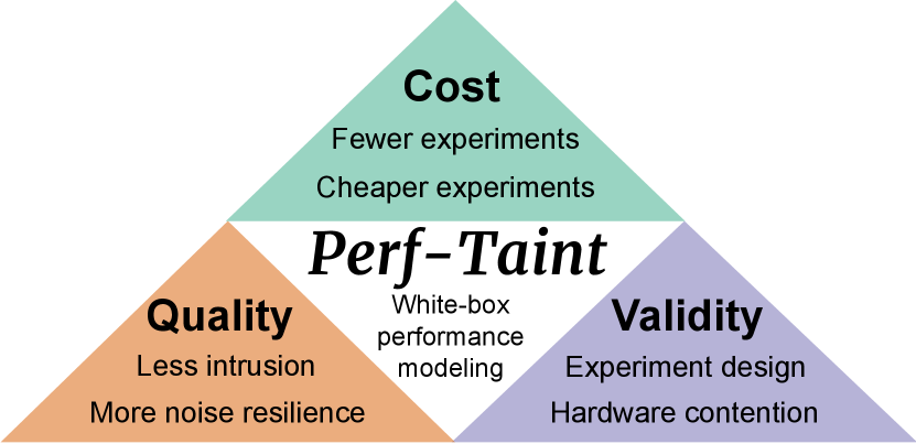
Figure 1. The basic concept of Perf-Taint. A tainted run of the program provides information that improves the empirical performance modeling process along the dimensions cost, quality, and validity of the resulting models.

In general, empirical performance modeling involves two important decisions: (1) choosing parameters that will affect application performance and (2) designing a set of experiments capable of accurately measuring their influence, while not exhausting the available computational budget.

Modern scientific applications use dozens of parameters that describe numerical properties, data size, or the degree of parallelism, making their selection extremely challenging. Without detailed insight into the application behavior, the user has to consider all possible combinations of the chosen parameters. The larger the number of parameters, the bigger is the number of experiments and the impact of noise on the quality of the resulting models (Ritter et al., 2020b). Some performance effects are not measurable for the entire range of parameter values available in the experiment design, potentially invalidating some measurements. Another major difficulty arises from the black-box nature of empirical modeling. Without insight into function behavior beyond empirical data, the modeler cannot distinguish between actual runtime change because of parameter influence and the effects of noise on the measurements. This leads to overfitting, estimating false dependencies, and generating incorrect models for constant functions with negligible execution time.

In this paper, we show how taint analysis (Clause et al., 2007a), a technique borrowed from the field of computer security, which reliably relates marked input values with the program parts they potentially affect, can provide this additional context, leading to the concept of tainted performance modeling. Performance tainting provides us with accurate performance parameter information and enables the design of a novel loop-based complexity analyzer. We integrate our complexity analyzer with Extra-P (Calotoiu et al., 2013a), an empirical performance-modeling tool, and derive a new hybrid performance modeling framework called Perf-Taint, whose underlying concept is illustrated in Figure 1. We make the following specific contributions:

• The application of taint analysis, which has originally been devised to track the flow of protected data through a program, to a new problem: the improvement of empirical performance models of HPC applications.

• The elaborate concept of tainted performance modeling, that can (1) reduce the cost of empirical performance models, (2) improve their quality, and (3) help validate them and the experimental setups used for their generation. An example of such a validation is the detection of contention as the source of measurements that contradict expected computational volumes.

• An open-source, LLVM-based tainted performance modeling tool, ready to use on HPC programs to provide the insights of a virtual performance expert.

After reviewing related work in Section 2, and the taint analysis in Section 3, we describe the theoretical and practical aspects of our method in Section 4 and Section 5, respectively. We then demonstrate the benefits it provides in Section 6 and present our conclusion in Section 7.

2. Related Work

The broad spectrum of existing methods and tools to support the creation of performance models documents their importance for understanding the performance influence of algorithms (Zaparanuks and Hauswirth, 2012), the hardware (Lo et al., 2014; Marin and Mellor-Crummey, 2004), and the operating system (Hammer et al., 2015; Zaparanuks and Hauswirth, 2012; Meswani et al., 2013). They are often used to extrapolate performance outside the known range of a single parameter (Zhai et al., 2010; Vuduc et al., 2004; Jayakumar et al., 2015) or even multiple parameters (Siegmund et al., 2015; Goldsmith et al., 2007), sometimes exploiting the properties of certain classes of algorithms such as stencil computations (Wu and Müller, 2012). Some require the prior annotation of the code with performance expressions (Tallent and Hoisie, 2014; Spafford and Vetter, 2012). Machine learning methods have also been successively used for performance modeling (Ipek et al., 2005; Lee et al., 2007).

There have been several attempts to enable performance modeling through static analysis of source code (Kuhnemann et al., 2004; Meng and Norris, 2017; Lee et al., 2015; Gschwandtner et al., 2018). Thanks to the dynamic nature of taint analysis, our method is not affected by fundamental limitations of static methods. The dependence of performance modeling tools on an entirely static dataflow analysis or a perfect loop modeling might prevent them from scaling to large scientific applications. A hybrid performance modeling tool was presented for online modeling by Bhattacharyya et al. (Bhattacharyya et al., 2015).

A different aspect of performance modeling, dataflow analysis, is also well studied in high-performance computing: DfAnalyzer performs dynamic dataflow analysis of Spark high-performance applications (Sousa et al., 2018). Parallel control-flow graphs of MPI programs have been constructed with dataflow analysis (Aananthakrishnan et al., 2013). Value influence analysis, a variant of taint analysis, has been used in message-passing applications (Roth and Meredith, 2014).

3. Dynamic Taint Analysis

When trying to construct the performance model of a full application, one would hope that there is a way to automatically determine its runtime complexity (or complexity w.r.t. other metrics) by analyzing the program code with a sufficiently smart compiler. While previous research showed first results (Hoefler et al., 2010) towards this direction, these solutions are inherently limited to special cases or approximations and are hard to scale to non-trivial programs (Section 3.1), as even the simple problem of identifying which input parameter affects an arbitrary program variable is inherently difficult.

Dynamic taint analysis (Section 3.2) has been successfully used in the context of computer security to reliably analyze data relations across complex programs. We introduce the major concepts and techniques and discuss how taint analysis provides precise knowledge as to how input parameters affect variables of the program. This gives us the instruments to introduce white-box performance modeling of non-recursive HPC programs (Section 4).

3.1. Static performance modeling is hard

Modeling performance statically is difficult from both a theoretical and a practical viewpoint. There are strict theoretical limitations of how accurate a static analysis can be or if an analysis can be computed at all. On the practical side, various levels of abstractions or indirections make program code easy to maintain, but make static analysis even less likely to succeed. We now outline several theoretical and practical considerations that make static performance modeling hard.

Theoretic limitations

There are strong theoretic reasons why static program analysis techniques are often unable to provide precise answers even for seemingly simple analyses. The most well known is the halting problem (Church, 1936) or its generalization, Rice’s theorem (Rice, 1953), which we here rephrase in the terms of program analysis: any non-trivial semantic property of a program cannot be computed. A property such as “does a program contain a certain instruction sequence” is syntactic and might be decidable, but “does a program return 0” is a semantic property and is undecidable for arbitrary programs. As a result, the question “can the value stored in a given memory location affect an instruction that is run when executing a given program” is a semantic property. Hence, determining whether a configuration parameter affects certain parts of a program is undecidable.

Practical considerations

While Rice’s theorem shows that the proof of semantic properties to be impossible for all programs, there might still exist a sufficiently large set of programs where this is realistic. We now argue that even an approximate analysis for only a subset of programs is difficult in practice. The main culprits are abstraction overhead, complex abstract data types, and runtime configurability. Abstraction is important to ensure the maintainability of large software projects. To that end, class hierarchies, virtual dispatching, and many very fine-granular functions are commonly used. As an example we show a simple matrix initialization in C99 and C++ (even avoiding the use of modern C++ constructs such as lambdas, range loops, etc.):

⬇

void init_c99(int Rows, int Columns,

float A[Rows][Columns], float val) {

for (int i = 0; i < Rows; i++)

for (int j = 0; j < Columns; j++)

A[i][j] = val;

}

class matrix {

int Rows, Columns;

float *A;

public:

float &at(unsigned i, unsigned j) {

return A[i * Columns + j];

}

unsigned getColumns() { return Columns; }

unsigned getRows() { return Rows; }

};

void init_cpp(matrix &A, float val) {

for (int i = 0; i < A.getRows(); i++)

for (int j = 0; j < A.getColumns(); j++)

A.at(i,j) = val;

}

While the initialization routine looks very similar in both cases, deriving the number of loop iterations is significantly more complicated for the C++ function. In the C99 variant, the number of rows in the matrix $A$ is directly available as a raw integer variable. In contrast, the C++ variant of this code encapsulates this information in the matrix data structure. Compilers are certainly good at reducing abstraction overheads and especially C++ is known as a language to make this easy. However, compilers such as LLVM or gcc do not reliably eliminate the abstraction overhead even in this simple example. There are two main problems that make eliminating this overhead difficult: (1) the matrix itself is passed as a pointer, and the size of the matrix is stored in memory as member of the struct describing an instance of the class matrix. Simplifying code with double pointer indirection requires a very good understanding of pointer aliasing; (2) the type of the matrix is part of the calling convention, hence the compiler is not allowed to change it if it appears in a library interface.

Pointer aliasing in general is a hard problem, where the most advanced inter-procedural techniques (Steensgaard, 1996) are still very imprecise (Shapiro and Horwitz, 1997) on large code bases. In practice (e.g., LLVM), only very limited intra-procedural pointer-alias analyses are run, as the minor increase in precision does not justify the large compile-time cost to run them. Similarly, today’s compilers only carefully inline function calls as otherwise code size (as well as compile time and runtime) grows uncontrollable. As a result, almost any analysis becomes inter-procedural and in this setting virtual function calls (or exceptions) make it even more challenging to understand statically how data flows in a program.

Another source of over-approximation is the hard-to-predict control-flow found in languages gaining popularity in scientific computing. The problem arises from virtual dispatch in statically typed languages (C++, Julia) and from duck typing (Python).

Message-passing and multithreading adds to the code non-determinism that can lead to a combinatorial explosion of states. A common choice for the analysis of MPI programs is symbolic execution (Fu et al., 2015), but it suffers from the exponential number of paths it has to analyze, limiting its scalability (Yu, 2018).

3.2. Dynamic taint analysis

Dynamic taint analysis is a runtime analysis that marks and tracks the movement of certain data elements and computed results depending on them through the execution of a program. Taint analysis can compute semantic analyses while a program is executed, overcoming the limitations that prevent static (compile-time) analysis from providing precise results, at the price of narrowing the insights to a specific run and its input configuration. For many analyses – especially if the results anyhow depend on input data – this is often exactly what is desired. We introduce a general taint-analysis framework that can be used to instantiate problem-specific taint analyses. We define three major components described by Clause et al. (Clause et al., 2007a) – (a) taint sources, (b) propagation policy, (c) taint sinks, which we discuss below with code examples.

Taint sources

Taint sources are all components of a program that can represent some kind of program data. Typical taint sources are memory locations, variable names, or function return values, but almost any part of a program can be a taint source, including I/O interfaces, system calls, network devices, etc. Marking taint sources requires the specification of data to be tainted and taint labels used to mark it. ⬇ // Program input: taint with label ”size” scanf(”%d”, &size); // Manual taint source: taint with label ”p” write_label(&p, sizeof(p), ”p”); // Third-party library output: taint with label ”ranks” MPI_Comm_size(MPI_COMM_WORLD, &ranks);

Taint propagation policy

The taint propagation policy defines how taint labels are moved through a program. We specify it by (1) defining a mapping function, and by (2) defining the affected data. The mapping function defines how two (or more) taint labels are joined. In the most trivial case, two sets of labels are joined by taking the union of the sets.

The affected data defines all data to which taint labels are propagated through data-flow and control-flow. Data-flow based propagation passes taint labels from inputs of operations to their outputs, including program instructions and propagation from function arguments to its return value. Control-flow based propagation captures the propagation of taint labels through control dependencies (Kang et al., 2011; Clause et al., 2007b).

⬇

int foo(int a,int b,int c) {//Input labels: ”a”,”b”,”c”

int d = 2 * a; //Dataflow tainting with label ”a”

if(b) d++; else d–; //Explicit tainting, label ”b”

if(c) d = pow(d, 2); //Implicit tainting, label ”c”

return d; //Taint labels of return: ”a”, ”b”, ”c”

}

In the example above, the variable a taints the return value of the function through a data-flow propagation. Variable b taints d through a control-flow condition which controls the execution of code that changes the return value (explicit dependence). An implicit dependence occurs for c since the value depends on it even if the second branch is not taken.

Taint sinks

Taint sinks are program code locations with an associated variable or memory location that may observe tainted program data. Sinks are used to determine which tainted values affect a given behavior. Each taint sink is defined by (1) a program code location, (2) the variable or memory location to check, and (3) a checking method that is invoked whenever the taint sink is executed. The checking method is supplied with program variable and associated taint labels on invocation. Whenever a taint sink’s checking method is invoked, it is supplied with the variable or memory location to check together with the set of associated labels.

⬇

if(result > threshold) {

handle_edge_case();

sink({&result, &threshold}, edge_case_handler);

}

4. Tainted Performance Modeling

Building on the concepts presented in Section 3.2, we introduce a taint analysis for performance modeling (Section 4.1), where the influence of input parameters on program variables is used to model the number of loop iterations. We show how this knowledge allows us to place a bound on the volume of computation (Section 4.2), defined as the number of operations executed in a non-recursive program run. An empirical black-box performance modeler uses the information of compute volumes to limit the space of potential complexity functions it considers (Section 4.5).

4.1. Loop count parameter identification

We solve the core data-flow problem behind performance modeling by formulating a suitable taint analysis. We assume that all target metrics, such as the program runtime or the number of operations, only vary with the iteration number of loop constructs in the code. This assumption is intuitive because the source code is typically not changed (i.e., in complexity or size) when changing program input parameters. Our analysis computes how potential input parameters affect the iteration counts of all natural loops (Aho et al., 1986) in a program. While the analysis does not support recursive functions, it warns of over-approximation when recursion is detected. Nevertheless, the core focus of performance modeling are HPC applications where the vast majority of computations are iterative anyway.

Sources

The sources of our loop taint analysis are all potentially performance-relevant parameters of a program. Performance relevant parameters are all memory locations marked explicitly by the performance engineer with a parameter label. Parameters are typically read from the command line, but might also be provided through other means (e.g., a configuration file), as long as their value is eventually stored in a variable that the user has marked as a parameter.

Propagation policy

To reliably produce accurate results, our analysis requires the propagation of taint across data flow and control flow. Because we need to know only the presence of a specific taint label in a performance-relevant variable, we choose the set union as mapping function. Each label will contain the set of input parameters that in some way affected the value marked by the taint label.

Sinks

The sinks of our taint analysis are all loop exit conditions. For a given loop, the number of times it iterates depends only on loop exit branch conditions. Any further indirect dependencies will eventually taint these branch conditions through our taint analysis.

We summarize the concepts in an example. With automatic taint propagation, the dependency on input parameters is propagated through function calls and memory operations to the sink, where it is used by our loop-count analysis. ⬇ struct params = parse_args(); write_label(&params.size,”size”, &params.step,”step”); iterate(pow(params.size, 2), optimize_step(params)); void iterate(int size, int step) { for(int i = 0; i < size; i += step) { compute(); sink({&i, &size}, register_loop); } } Assuming a loop $L$ depends on taint labels $p_{1},\dots,p_{n}$, the number of loop iterations of $L$, $count(L)$, must then be a function $g(p_{1},\dots,p_{n})$. While the parameters this function potentially depends on are clearly defined, no further information about function $g$ can be derived through the taint analysis itself. Even if the taint label just contains a single taint mark $p$, it does not imply a number of loop iterations linear in $p$. $count(L)$ could also be $log(p)$, $p^{2}$, or any other function $g(p)$. As a result, we can state the following claim:

Claim 1.

Given an application with a set of input variables V and a set of $n$ correctly marked potential performance variables $P=(p_{1},\dots,p_{n})\subseteq V$, we derive for a given loop $L$ a class of symbolic functions $g_{i}(p_{1},\dots,p_{n})$ which only depend on parameters in $P$. If all program parameters that impact the iteration count of $L$ have been marked, a performance taint analysis with full data and control flow propagation computes with $count(L)=p_{i}$ a class of functions which contain the function that exactly describes the number of loop iterations.

4.2. Iteration volume of a loop nest

We now derive the iteration volume of a loop nest, that is, the accumulated number of times the body of a loop nest is executed. We define the iteration volume recursively. The base case of our recursion is a loop nest with just a single loop $L$. In this case, the volume of computation $vol(L)$ is $count(L)=g(\vec{p})$, the result of our loop iteration count parameter identification. We now define the iteration volume of larger loop nests by combining existing loop nests.

Sequencing two loops

Executing two child loops nests ($LN_{c1}$ and $LN_{c2}$) in sequence forms a larger loop nest $LN$. The iteration volume of $LN$ is over-approximated as the sum of the compute volumes of the child loop nests, $vol(LN)=vol(LN_{c1})+vol(LN_{c2})$.

⬇

LN: {

for(int i = 0; i < count(LN_c1); i += 1) { … }

for(int i = 0; i < count(LN_c2); i += 1) { … }

}

Nesting of a loop and a loop nest

Executing a child loop nest ($LN_{c}$) inside a loop $L$ forms a larger loop nest $LN$. The iteration volume of $LN$ is over-approximated by multiplying the iteration count of the outer loop with the iteration count of the loop nest, $vol(LN)=g(\vec{p})\cdot vol(LN_{c})$.

⬇

LN: {

L_1: for(int i = 0; i < count(L_0); i += 1)

for(int j = 0; j < count(LN_child); j += 1)

…

}

The power of these simple composition rules can be summarized in the following claim about asymptotic performance with respect to performance-critical variables.

Claim 2.

Given an application with a set of input variables V, a set of $n$ correctly marked potential performance variables $P=(p_{1},\dots,p_{n})\subseteq V$, and a loop nest built from natural loops $L_{i}$ without irreducible control flow or recursion, we derive for the loop nest a class of symbolic functions $g_{i}(p_{1},\dots,p_{n})$ which only depend on the parameters in $P$. If all variables that impact the loop iteration count have been marked, we derive an asymptotic upper bound on the maximal number of times any given basic block is executed in the loop.

These functions may still contain unresolved functions $g(\vec{p})$ representing loops for which the runtime is not known statically. We will explain in Section 4.5 how we derive these functions empirically from performance measurements.

4.3. Compute volume of a full program

We calculate the compute volume of a full program without recursion. Any code not part of a loop can be ignored as it has only constant cost. Similarly, bodies of inner loops can be assumed to have only constant computational cost since the analysis is inter-procedural and loop nests are aggregated across function calls. Therefore, the asymptotic compute volume can be derived by looking only at the recursively accumulated cost of loop nests.

Theorem 1.

Given an application $A$ with a set of input variables V, a set of $n$ correctly marked potential performance variables $P=(p_{1},\dots,p_{n})\subseteq V$, no irreducible control flow or recursion, the recursive accumulation of the iteration volume in each function of the call tree (due to no recursion) computes the asymptotic compute volume of $A$.

The taint analysis therefore yields properties of the function space of possible performance models but it does not explicitly generate precise models. In this sense, it provides a “scaffolding” that defines some relations among loops. However, the precise function for each loop is not yet defined. To derive such functions, we first discuss how to include additional control-flow information into the model (4.4). We subsequently refine an empirical modeling approach to parametrize the missing loop models to derive accurate overall performance models for each function (4.5).

4.4. Algorithm selection

In addition to building a set of performance models for each function discussed earlier, we apply taint analysis to locate control-flow decisions unrelated to loop exit conditions that are affected by input parameters. Instrumenting conditional branches with taint sinks enables (1) the detection of tainted control-flow decisions affecting performance models for branches inside any loop nest and (2) the detection of code paths that are never visited, including the parameter-based selection of algorithms.

4.5. Empirical performance modeling is also hard

Our dynamic taint analysis provides us with information on how parameters influence the compute volume of individual functions, but does not provide specific functions that describe the asymptotic behavior very precisely. To close this gap, we build a hybrid analysis by combining the compute volume information from our compiler-based analysis with a black-box empirical performance modeler. This modeler runs a program multiple times with different parameter configurations. Using both the results of taint analysis and the observed execution times, it derives a performance-model function that (1) respects parameter dependencies derived during the taint analysis and (2) provides the best fit to empirical data. As a black-box performance prediction approach we use the performance modeling tool Extra-P (Calotoiu et al., 2013b; Shudler et al., 2015; Calotoiu et al., 2016).

Performance function

A key concept of the Extra-P approach is the performance model normal form (PMNF), defined in Equation 1. It models the effect of parameters $x_{i}$ on a variable of interest $f(x_{1},\dots,x_{m})$, typically execution time or a performance counter. The PMNF is based on the assumption that performance, at least at the level of functions calls, can usually be expressed as a combination of polynomial and logarithmic terms. This flexibility in expressing behaviors is sufficient to cover most cases encountered in practice while keeping the modeling process fast enough to be viable.

(1) $$f(x_{1},\dots,x_{m})=\sum_{k=1}^{n}c_{k}\cdot\prod_{l=1}^{m}x_{l}^{{i_{k}}_{l}}\cdot log_{2}^{{j_{k}}_{l}}(x_{l})$$

The PMNF defines a function search space, which is traversed to find the function that comes closest to representing the set of measurements. This assumes that the true function is within the search space. A possible assignment of all $i_{k}$ and $j_{k}$ in a PMNF expression is called a model hypothesis. The sets $I,J\subset\mathbb{Q}$ from which the exponents $i_{k}$ and $j_{k}$ are chosen and the number of terms $n$ define the model search space. The coefficients of all hypotheses are automatically derived using regression and the hypothesis with the smallest error is chosen to find the most likely model function. In this work, we use the configuration suggested by Ritter et al. (Ritter et al., 2020b).

This approach always generates a human-readable expression out of any given measurement data. It attempts to explain this data as well as possible by fitting the PMNF to the data. The more complex the PMNF is, such as by adding more terms or a wider range of exponents to the terms, the more freedom the modeling has to fit the data. This allows more behaviors to be expressed but risks overfitting the data—especially in the presence of noise.

Search space

In practice, a simple selection like the following is often sufficient to model even complex scientific applications:

$$n =2$$

$$I =\left\{\frac{0}{4},\frac{1}{4},\frac{1}{3},\frac{2}{4},\frac{2}{3},\frac{3}{4},\frac{4}{4},\frac{5}{4},\frac{4}{3},\frac{6}{4},\frac{5}{3},\frac{7}{4},\frac{8}{4},\frac{9}{4},\frac{10}{4},\frac{8}{3},\frac{11}{4},\frac{12}{4}\right\}$$

$$J =\{0,1,2\}$$

It is possible to expand or modify the sets or the number of terms if clear expectations regarding the application behavior exist, but such prior knowledge is not required in the common case. For the above process to yield good results, the true function that is being modeled should not be qualitatively different from what the normal form can express. Discontinuities, piece-wise defined functions, and other behaviors that cannot be modeled by the normal form will lead to sub-optimal results. Looking at Equation 1, the combinatorial explosion of the search space for model hypotheses becomes apparent when using the same assumptions regarding hypotheses generation as we did in the single-parameter case. With as few as three parameters, the model search space contains more than $10^{14}$ candidates, making the search for the best fit a daunting task. Extra-P includes two heuristics that deal with the excessive size of the search space. The first heuristic speeds up multi-parameter modeling, as it reduces the search space to only combinations of the best single-parameter models. The second heuristics speeds up model selection for single parameter models. Combined, the two heuristics allow a search space of hundreds of billions of models to be reduced to under a thousand (Calotoiu et al., 2016).

Limitations

A significant limitation of Extra-P is the black-box nature of the approach that uses only empirical measurements to generate performance models. This means that the models can be affected both by random noise, and by systemic interference such as network congestion caused by multiple applications sharing a physical system. While these effects can be mitigated by repeating measurements and trying to control the measurement infrastructure, they cannot be eliminated and their impact is larger the more parameters are considered (Ritter et al., 2020b). In most applications, runtime is concentrated in a small number of routines, and while these routines are correctly modeled, the previously discussed disturbances disproportionately affect regions of code with short runtimes, and in some cases translate to Extra-P effectively modeling noise. Given the large number of such occurrences, in some the noise can randomly resemble a strong correlation between a parameter and a metric. Such false positives can, at the moment, only be eliminated by manual inspection of the code and cost users valuable time.

Hybrid modeler

Our goal is to allow the PMNF to be as expressive as possible to accurately model different performance behaviors but wish to prevent this expressivity from generating false positives by overfitting. We therefore use taint analysis to define a prior for the modeling process in Extra-P. We use the results of the taint analysis to minimize the negative effects of measurement noise. The model of computational volume is applied to restrict the search space by removing parameters that could not affect performance. As a result, the black-box regression algorithm no longer uses non-existing parameter dependencies in models.

The immediate effect is pruning out parametric models for constant functions. These functions are notoriously hard to model since the variability of measurement data forces the modeler to favor functions that are not constant. The final model is overfitted and likely misleading. The second important result is the removal of false dependencies in performance models. We therefore automate the process of verifying empirical models by removing parameters not present in the code from the search space.

5. Implementation of Perf-Taint

We provide with Perf-Taint an implementation of our performance tainting approach, as shown in Figure 2. Our processing pipeline includes the new step of tainted modeling that consists of three stages: (1) a static analysis, (2) a dynamic taint analysis; and (3) a database of performance-critical libraries, which we discuss in detail in the following subsections. Perf-Taint uses LLVM (Lattner and Adve, 2004) and works on the level of the intermediate representation (IR), which makes Perf-Taint applicable to a range of languages, including C++, Fortran, Julia, etc. However, our taint-based modeling approach (Section 4) is independent of the taint implementation and can also be built using other taint-analysis frameworks (Kang et al., 2011; Kemerlis et al., 2012; She et al., 2019; Clause et al., 2007b).

Figure 2 shows how performance modeling with Extra-P is improved with the program information provided via taint analysis. Without taint analysis expert knowledge is necessary to decide which parameters have the largest impact on performance and scalability, a difficult manual task. Perf-Taint leverages taint analysis to determine how many loops and functions are affected by each specific parameter, providing a simple yet intuitive coverage metric and removing from the analysis any parameters that have no effect on performance. The only user action is the annotation of each input parameter with one line of code in the program source, as illustrated in the example below. In contrast to many performance modeling tools (Tallent and Hoisie, 2014; Meng and Norris, 2017; Lee et al., 2015), we do not require our users to annotate regions of interests, functions, loop boundaries, or even to provide manually annotated performance models for each kernel.

⬇

struct cmdLineOpts opts;

ParseCommandLineOptions(argc, argv, myRank, &opts);

register_variable(&opts.nx, ”size”);

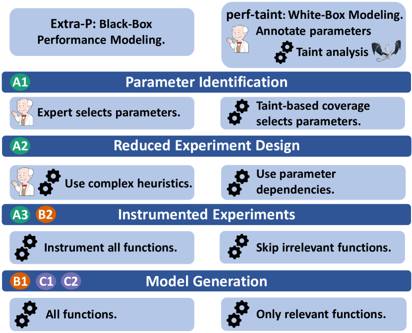
Figure 2. The processing pipeline of Perf-Taint. All four major steps of empirical modeling are improved with the program information provided by taint analysis.

The next step determines the set of measurements used for empirical modeling. The user needs to provide the constraints on parameter values, which is a problem-specific part. The naïve approach considers all combinations of parameter values and therefore the number of samples scales exponentially with the number of parameters. While the original approach required sophisticated heuristics and a potential accuracy loss to reduce this number, taint analysis decides which parameter have multiplicative dependencies and which lead to additive effects. This means often not all combinations are required, therefore reducing the burden of the most computationally expensive part of the pipeline without sacrificing accuracy. Finally, Perf-Taint uses taint-based information on parameter dependencies to select only relevant functions for instrumentation and prune models with false dependencies, leading to better and cheaper models.

5.1. Static analysis

At compile time, we identify all functions that contain no loops or only loops with constant and statically resolvable trip counts since their performance models are known to be independent from any program parameter. To that end, we query an existing loop induction analysis (e.g., ScalarEvolution (Gohman, 2009)). During this process, we include functions containing library calls that are known to be affected by performance parameters, such as MPI communication routines.

5.2. Dynamic taint analysis

We build our solution on top of the DataFlowSanitizer plugin (dfsan, 2019) in the Clang and LLVM compiler toolkit, a data-flow taint system consisting of (1) a transformation pass applied to source code, and (2) a runtime library implementing label allocation, query, and union. The taint labels are designed as a tree-like data structure, where each label can represent a union of up to two labels. Each label has an associated 16-bit identifier. The union operation verifies whether the operands do not represent an equivalent combination of labels and creates a new one if necessary. While the implementation is less efficient than a simple bitset solution, it supports up to $2^{16}$ unique labels. The runtime manages the shadow memory pool that stores taint labels for each memory location of the program. The transformation pass instruments each instruction with propagation of taint labels from its operands to the output.

Perf-Taint gathers information on the effects of tainted parameters on each non-constant loop in the program, by treating loop exit branch conditions as taint sinks. We store call-path information to distinguish between function calls that result in different dependencies, letting the empirical modeler Extra-P create calling-context-aware performance models. As part of post-processing after program execution, we parse loop nests with parameter dependencies and use this information to generate explicit multiplicative and additive dependencies for a function. The only source of over-approximation in our analysis is the presence of multiple labels in a single exit condition, where we conservatively report a multiplicative dependency. The latter requires more experiments to be accurately parametrized.

Control-flow tainting

We extended DataFlowSanitizer with instrumentation for explicit control-flow tainting since it is necessary to capture all dependencies in real-world applications. Both the runtime and the transformation pass have been extended to store the taint labels associated with control-flow decisions, and propagate them to variables whose values depend on the control flow. Below, we present an example from the LULESH benchmark discussed in Section 6. The final value contained in regElemSize has a control dependence on parameter size through numElem in the loop condition, since the value depends on the number of loop iterations. This kind of dependency cannot be recovered by only considering data flow, i.e. the propagation of labels from instruction inputs to an output.

⬇

for(Index_t i = 0 ; i < numElem(); ++i) {

int r = this->regNumList(i) - 1;

regElemSize(r)++;

}

5.3. Global state libraries

Loop-based kernels are not the only way how parameters can affect the performance. The model has to include parametric effects of communication and synchronization routines. The performance parameter could affect their behavior in the following ways: (1) a value tainted by the parameter is exchanged between processes operating in disjoint memory spaces, (2) the parameter is passed to the routine explicitly, (3) the parameter is hidden from the user in the library runtime. We solve issues (2) and (3) by introducing a library database describing performance-relevant functions, implicit parameters provided by libraries, and sources of taint values.

We demonstrate the solution on MPI, the most widely-used library for distributed and high-performance applications. We declare the implicit parameter p, which denotes the size of the global communicator, and we include the function MPI_Comm_size as a source of tainted values, writing a label to the memory address passed as a second argument to the function. We derive parametric dependencies for MPI communication and synchronization routines from precise analytical models (Thakur et al., 2005; Hoefler and Moor, 2014), and provide them in the library database supplied with Perf-Taint. As an example, we consider the case of MPI peer–to–peer communication routines. When they appear in a function, our analysis introduces implicit dependence on p. Since performance of these functions depends on the network conditions and message size, we query the taint labels associated with count argument provided to the function and add them as additional parametric dependencies for this function call.

Taint labels could be transfered between processes withing MPI messages. The problem of tainting network communication has already been tackled (Zavou et al., 2011), and an analogous solution for MPI would only have to cover standard MPI datatypes and the few, well-defined routines that create user-defined datatypes. We have found that the lack of support for data exchange across the network is not an obstacle for the applications we analyzed.

6. Taint Analysis in Action

	Piz Daint	Skylake Cluster
CPU	Intel Xeon E5-2695 v4 2.10GHz	Intel Xeon 6154 3GHz
Cores	2 sockets, 18 cores each	36 cores
Memory	128 GB	384 GB
GCC, MPI	GCC 8.3, Cray MPICH 7.7.2	GCC 8.3, OpenMPI 4.0.3
Software	Score-P 6.0 (an Mey et al., 2012), Extra-P 3.0 (ext, 2018), LLVM 9.0 (Lattner and Adve, 2004)

Table 1. Software and hardware configuration of Perf-Taint evaluation on Piz Daint and a local Skylake cluster.

	LULESH	MILC
Functions	356	629
Pruned Statically/Dynamically	296/11	364/188
Kernels/Comm. Routines/MPI	40/2/7	56/13/8
Loops	275	874
Pruned Statically	52	96
Relevant	78	196
Modeling
p	$3^{n}(27,...,729)$	$2^{n}(4,...,64)$
size	25,30,35,40,45	32,64,128,256,512

Table 2. Overview of LULESH and MILC: the two-phase identification of computational kernels, communication routines and MPI functions used, and the manually specified parameter values for two-parameter modeling.

We present the three major categories of improvements that our taint-supported framework brings to the empirical performance modeling process: decreased cost (Section  ), improved quality (Section  ), and the discovery of software and hardware phenomena the knowledge of which can help validate experiment design and modeling results
 (Section  ). We support our claims by applying taint-supported performance modeling to two representative HPC benchmarks: LULESH (Karlin et al., 2013) and MILC (Bernard et al., 1991), summarized in Table 2 and discussed in the next two paragraphs. The hardware and software systems used are summarized in Table 1.

LULESH

is a scientific application written in C++, implementing stencil computations for a hydrodynamic shock problem on a three-dimensional mesh. The code is structured around the main class Domain and contains multiple simple methods. Their expected constant computational effort is hard to capture empirically because the presence of noise makes timing data unreliable for such short functions. We run the taint analysis of this application with size 5 and 8 MPI ranks, leaving other parameters at the default value, since it provides a representative execution of the application that is close to parameter configurations used in modeling (Section  ). If we choose the number of MPI ranks p and the grid size size as performance-model parameters, a typical use case, our analysis marks 86.2% of the functions as not influenced by these two parameters, allowing the immediate classification of their models as constant.

MILC

We model the performance of the su3_rmd application from the MIMD Lattice Computation, a collection of scientific applications working on problems from the lattice quantum chromodynamics (QCD) fields. We analyze here the effects of two parameters frequently chosen for scaling studies: (1) the size of the space-time domain, which is computed from the four parameters nx, ny, nz, and nt, and (2) p, the number of MPI ranks. We apply the taint analysis of this application with a size of 128 on 32 MPI ranks. Again, the taint analysis identifies 87.7% of the functions as constant relative to these two parameters. This corrects 77% models previously indicating performance effects. Our analysis is confirmed by the preceding manual analysis and the validation with up to 512,000 processes (Bauer et al., 2012).

LULESH Total p size regions iters balance cost p, size Functions 43 2 40 13 4 9 2 40 Loops 86 2 78 27 4 20 2 78 MILC Total p size trajecs warms nrest. mass,beta p, size steps niter nfl. / u0 Functions 56 54 53 12 9 6 1 / 4 56 Loops 196 187 161 39 31 15 1 / 7 196

Table 3. Computational kernels and loops in multi-parameter modeling. p, size is not equal to the sum of corresponding columns since multiple parameters can affect the same region.

   Cost

The cost of the modeling process is influenced by two major factors: the number of the required performance experiments, which significantly grows with the number of model parameters, and the cost of these experiments under instrumentation. Tainted performance modeling lowers these costs in multiple ways while reducing the dependence on human expertise. First, it supports automatic pruning of the parameter space (Section  ), avoiding many unnecessary experiments. It can expose parameter dependencies at an early stage (Section  ), allowing smarter experiment design with even less experiments. Finally, we show that the ability to judge the performance relevance of a function upfront substantially decreases the instrumentation overhead (Section  ).

   Parameter pruning

High-performance computing applications often involve a large set of execution parameters. In practice, limited compute budgets restrict the number of model parameters to three, and even with boundless resources one should not go much beyond, as the impact of noise would become too strong (Ritter et al., 2020a). Tainting allows us to decide which parameter influences which part of the program. Programmers should mark program parameters found in routines parsing command-line arguments and configuration files. Our analysis determines all parameters without effect on the control flow and counts the number of loops and functions directly affected by a specific parameter. Table 3 summarize parameter pruning on both benchmarks, excluding communication routines relevant only because of calls to MPI.

LULESH includes six major parameters: the problem size size, the number of MPI ranks p, regions, balance, cost, iters. To build a two-parameter model providing the broadest coverage of performance relevant functions our taint analysis suggests we select size and p.

In MILC, we detect the performance-relevant parameters nx, ny, nz, nt, steps, niter, warms, trajecs and the implicit parameter p. Our findings are identical with the ground truth established by experts in a laborious manual process (Bauer et al., 2012).

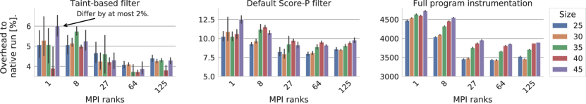
Figure 3. The Score-P instrumentation overhead of LULESH on the Skylake cluster. Plot scales are tuned to enhance visibility.

Figure 4. The Score-P instrumentation overhead of MILC on the Skylake cluster. Plot scales are tuned to enhance visibility.

   Parameter dependencies

Taint analysis can find parameter dependencies, such as multiplicative dependencies between parameters influencing the iteration count in outer and inner loops, and additive dependencies between parameters influencing the iteration count of non-nested loops. For routines where parameter dependencies are detected as additive only, accurate performance models can be generated by creating single parameter models for each of the parameters involved. Should this be true for all routines in an applications, the experiment design as a whole can be simplified and its dimensionality reduced.

An interesting corner case of a multiplicative dependency is LULESH, where the taint-based modeling detects a single instance of the parameter iters in the main loop of the program. Through that we recover a multiplicative dependency with all other model parameters. The number of iterations therefore linearly affects the entire computation. We can reduce the dimensionality of sample space, since iters does not grant useful insights into application performance.

   Instrumentation overhead

In the default instrumentation mode, Score-P (an Mey et al., 2012), a widely used measurement infrastructure and the default for Extra-P, estimates whether a function should be inlined and therefore excluded from instrumentation. This approach is inappropriate for empirical performance modeling because it might encourage the compiler to remove performance-critical functions through inlining, obscuring potential sources of bottlenecks and impeding effective performance analysis. Thus, without contextual information from the taint analysis, each function must be conservatively assumed to be influenced by changing parameter values, leading to instrumentation of all functions and significant runtime overhead.

Using the results of our analysis, we decrease the instrumentation overhead by instrumenting selectively, including only functions that are affected by a parameter change. In particular, we prune most of the simple constant functions, such as class getters and setters, which are irrelevant to scaling studies, without reducing the model quality for the remaining functions. We compare the overhead of Score-P with default, full, and our selective instrumentation.

The results for LULESH in Figure 3 clearly demonstrate how severe the overhead can become for C++ applications. Depending on the number of ranks and the problem size, removing constant and irrelevant functions decreases the execution time by a factor of up to 45 times. Although the overhead of the default Score-P instrumentation is manageable, the results may influence the models themselves. Our selective instrumentation contains 40 important application functions, while the default Score-P run instruments less than half of the performance-relevant functions but includes helper functions with constant runtime. The results for MILC are presented in Figure 4. There, the geometric mean of overheads are $1.6\%$ for selective instrumentation and $23\%$ for full and default instrumentation. The default instrumentation provides little to no benefit, whereas the overheads of our instrumentation are negligible on larger-scale runs. We observe that selective instrumentation provides the most significant improvements in C++ applications, which are gaining popularity in the HPC community.

Since the default Score-P instrumentation misses important functions, causing false-negative results, the modeling process can only use a full instrumentation mode. The core-hour costs of taint analysis are 1 and 16 hours for LULESH and MILC, respectively, while the costs of the experiment decreased from 20483 to 547 hours for LULESH (97.3%), and from 364 to 321 hours for MILC (13.4%), when switching from a full to taint-based instrumentation. The savings from reduced overhead significantly outweigh the costs of an additional analysis.

   Quality

We use tainting to mitigate the effects of measurement noise
 (Section  ), and the selective instrumentation discussed in Section  to reduce the intrusion of instrumentation, improving the quality of the resulting models (Section  ).

   Noise resilience

We apply the model obtained by the taint analysis to the model estimation in Extra-P, to prune models with false dependencies and evaluate the validity of experiments. We combine the five values of each parameter defined in Table 2 to construct a set of training data with 25 points, repeating each measurement five times to reduce the effects of random noise, resulting in 125 measurements, which we obtain by using up to 21 (LULESH) and 2 (MILC) Piz Daint nodes.

We compare the new models to black-box ones. We generally observe that models generated using taint analysis are closer to (nearly always exactly matching) the ground truth that we established with manual performance modeling techniques using code inspection (Hoefler et al., 2011). We select for the comparison only those functions whose data sets do not contain values with a coefficient of variance larger than $0.1$, as they are too affected by noise to be reliable.

We compare our findings for MILC with models created manually (Bauer et al., 2012) as a ground truth. For the kernels manually studied, the taint analysis correctly identifies the dependencies on both p and size in accordance with the theoretical study. The empirical model also converges to the same model for each function. There are four MPI_Comm_Rank functions which we correctly detect as constant where measurement noise previously caused incorrect models to be generated.

   Less intrusion

Empirical performance modeling relies on measurements. The instrumentation process introduces overhead, increasing the cost of the experiments, as discussed in the previous section. Yet, even more troubling is that the instrumentation perturbs the measurements, causing the resulting models to change qualitatively. We compare models from the fully instrumented code with those from code where only the routines identified as performance relevant are instrumented. Beyond the observation that nearly all runtimes are almost two orders of magnitude bigger under full instrumentation, critical routines such as CalcQForElems show different models depending on the degree of instrumentation. The model derived from fully instrumented runs shows an additive dependency between $p$ and $size$, $3\cdot 10^{-3}\cdot p^{0.5}+10^{-5}\cdot{size}^{3}$ while the filtered instrumentation shows a multiplicative dependency $2.4\cdot 10^{-8}\cdot p^{0.25}\cdot{size^{3}}$. The second model is validated by previously determined models (Calotoiu et al., 2018b), providing a strong argument for using a targeted approach towards instrumentation rather than simply instrumenting full applications. The default Score-P filter does not instrument this function, leading to false-negative result in this case.

   Validity

The empirical approach we study always generates a performance model from a given input. We previously discussed in Section  ‣ 6 how we can make sure that we generate the best possible model. There are situations, however, where the systemic influence of hardware or poor experiment design make the data unsuitable for understanding algorithmic performance. We identify such cases and provide guidance to identify the cause of the issue. We discuss two such examples: the effect of hardware contention in a multi-core system (Section  ), and a qualitative change in the modeled function across the experiment (Section  ).

   Detecting hardware contention

We evaluated the black-box and white-box modeling approaches with measurements of LULESH from Table 2. We observed a significant number of computational kernels, where the new model is worse at fitting the data even though it no longer contains false dependencies on p. Since the taint analysis proved that such functions cannot include such a dependency, yet it is visible in measurements, we conclude that that the resulting performance model must be affected by factors outside the application code itself. The taint-based modeling pipeline detects the presence of this perturbation while it was unknown to the black-box modeling approach.

We formulate the hypothesis that the co-location of MPI ranks on the same socket leads to hardware contention effects on functions with no dependence on MPI ranks in the source code. We test this hypothesis with a new experiment keeping the number of MPI ranks and problem size constant ($\texttt{p}=64$ and $\texttt{size}=30$) and varying the numbers or MPI ranks per node r, scaled from 2 to 18. By disabling multithreading, the larger number of cores available to each MPI rank should not affect the performance of compute kernels, and only communication routines might benefit from optimized MPI operations when processes are co-located. The expectation is that non-communication routines should have constant models. The entire application shows a significant increase in execution time, by 50%, from $130$\mathrm{s}$$ to $195$\mathrm{s}$$, with the corresponding model $2.86\cdot\log_{2}^{2}{\texttt{r}}$\mathrm{s}$+127$\mathrm{s}$$. Out of 73 functions, 31 have an increasing model with statistically sound measurements. Figure 5 shows a few major examples.

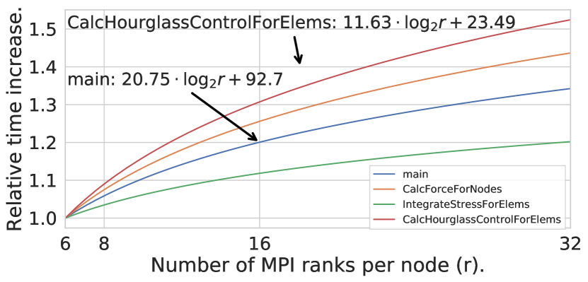
Figure 5. The one-parameter model of LULESH evaluating the effect of the number of MPI ranks r per node. Computational kernels experience slowdown because of hardware contention when many processes occupy the same socket.

Given the significant number of memory operations in the program, the saturation of memory bandwidth is the most likely culprit. Thanks to the inclusion of program information from taint analysis, we provide a type of insight that has not been available with purely black-box performance modeling. Modeling results that are independent of hardware effects and parallel allocations are possible for LULESH but only for certain levels of node saturation with MPI processes.

   Validating the experiment design

We evaluated the black-box and white-box modeling approaches with MILC test runs and noticed the largest difference between models of communication routines such as MPI_Isend and a MILC internal implementation of the gather collective operation.

Although the measurements are statistically valid, they fail to present a consistent behavior across the modeling domain. We notice a qualitative, not merely a quantitative difference between execution on 4, 8, 16 and larger numbers of ranks. As there is more than one behavior to be modeled in one interval, the parametric models estimated by Extra-P cannot represent the function accurately unless more measurement data is provided (Ilyas et al., 2017).

We have expanded our taint analysis to provide information regarding branches of code that are executed or not executed and therefore where application and/or library behavior can qualitatively change. This empowers the user to appropriately design his experiments to ensure there is only one behavior present in the data.

7. Conclusion

This work is the first to show that taint analysis, a method originally introduced to track the flow of sensitive information in computer programs, can be used to significantly advance the state of the art in empirical performance modeling for HPC applications. We showed various use-cases to improve cost, quality, and validity of the resulting models. Cost is reduced by lowering the number of necessary experiments as well as making individual experiments cheaper. Moreover, higher noise resilience and less instrumentation-induced intrusion render the models more accurate. Finally, with its ability to approximate the computational volume of program executions, taint analysis can help expose contention effects that prolong the runtime beyond what one would expect from considering computational volumes alone. Overall, our results show that for applications of realistic complexity empirical modeling must be carefully combined with static and compiler-assisted dynamic analyses to deliver high-quality and actionable performance models.

- (1)
- ext (2018) 2018. Extra-P 3.0. http://www.scalasca.org/software/extra-p/download.html.
- Aananthakrishnan et al. (2013) Sriram Aananthakrishnan, Greg Bronevetsky, and Ganesh Gopalakrishnan. 2013. Hybrid Approach for Data-flow Analysis of MPI Programs. In Proceedings of the 27th International ACM Conference on International Conference on Supercomputing (Eugene, Oregon, USA) (ICS ’13). ACM, New York, NY, USA, 455–456.
- Aho et al. (1986) Alfred V. Aho, Ravi Sethi, and Jeffrey D. Ullman. 1986. Compilers: Principles, Techniques, and Tools. Addison-Wesley Longman Publishing Co., Inc., Boston, MA, USA.
- an Mey et al. (2012) D. an Mey, S. Biersdorff, C. Bischof, K. Diethelm, D. Eschweiler, M. Gerndt, A. Knüpfer, D. Lorenz, A. D. Malony, W. E. Nagel, Y. Oleynik, C. Rössel, P. Saviankou, D. Schmidl, S. S. Shende, M. Wagner, B. Wesarg, and F. Wolf. 2012. Score-P: A Unified Performance Measurement System for Petascale Applications. In Proc. of the CiHPC: Competence in High Performance Computing, HPC Status Konferenz der Gauß-Allianz e.V., Schwetzingen, Germany, June 2010. Gauß-Allianz, Springer, 85–97. https://doi.org/10.1007/978-3-642-24025-6_8
- Bauer et al. (2012) G. Bauer, S. Gottlieb, and T. Hoefler. 2012. Performance Modeling and Comparative Analysis of the MILC Lattice QCD Application su3 rmd. In Proc. of the 2012 12th IEEE/ACM International Symposium on Cluster, Cloud and Grid Computing (CCGrid) (Ottawa, Canada). IEEE Computer Society, 652–659.
- Bernard et al. (1991) Claude Bernard, Michael C. Ogilvie, Thomas A. Degrand, Carleton E. Detar, Steven A. Gottlieb, A. Krasnitz, R.L. Sugar, and D. Toussaint. 1991. Studying Quarks and Gluons On Mimd Parallel Computers. Int. J. High Perform. Comput. Appl. 5, 4 (Dec. 1991), 61–70.
- Bhattacharyya et al. (2015) A. Bhattacharyya, G. Kwasniewski, and T. Hoefler. 2015. Using Compiler Techniques to Improve Automatic Performance Modeling. In 2015 International Conference on Parallel Architecture and Compilation (PACT). 468–479.
- Calotoiu et al. (2016) Alexandru Calotoiu, David Beckingsale, Christopher W. Earl, Torsten Hoefler, Ian Karlin, Martin Schulz, and Felix Wolf. 2016. Fast Multi-Parameter Performance Modeling. In Proc. of the 2016 IEEE International Conference on Cluster Computing (CLUSTER), Taipei, Taiwan. IEEE Computer Society, 172–181.
- Calotoiu et al. (2018a) Alexandru Calotoiu, Alexander Graf, Torsten Hoefler, Daniel Lorenz, Sebastian Rinke, and Felix Wolf. 2018a. Lightweight Requirements Engineering for Exascale Co-design. IEEE. To appear in IEEE International Conference on Cluster Computing (Cluster’18).
- Calotoiu et al. (2018b) Alexandru Calotoiu, Alexander Graf, Torsten Hoefler, Daniel Lorenz, Sebastian Rinke, and Felix Wolf. 2018b. Lightweight Requirements Engineering for Exascale Co-design. In Proc. of the 2018 IEEE International Conference on Cluster Computing (CLUSTER), Belfast, UK. IEEE, 1–11.
- Calotoiu et al. (2013a) A. Calotoiu, T. Hoefler, M. Poke, and F. Wolf. 2013a. Using Automated Performance Modeling to Find Scalability Bugs in Complex Codes. IEEE/ACM International Conference on High Performance Computing, Networking, Storage and Analysis (SC13).
- Calotoiu et al. (2013b) Alexandru Calotoiu, Torsten Hoefler, Marius Poke, and Felix Wolf. 2013b. Using Automated Performance Modeling to Find Scalability Bugs in Complex Codes. In Proc. of the ACM/IEEE Conference on Supercomputing (SC13), Denver, CO, USA. 1–12.
- Church (1936) Alonzo Church. 1936. An unsolvable problem of elementary number theory. American journal of mathematics 58, 2 (1936), 345–363.
- Clause et al. (2007a) James Clause, Wanchun Li, and Alessandro Orso. 2007a. Dytan: a generic dynamic taint analysis framework. In Proceedings of the 2007 international symposium on Software testing and analysis. ACM, 196–206.
- Clause et al. (2007b) James Clause, Wanchun Li, and Alessandro Orso. 2007b. Dytan: A Generic Dynamic Taint Analysis Framework. In Proceedings of the 2007 International Symposium on Software Testing and Analysis (London, United Kingdom) (ISSTA ’07). Association for Computing Machinery, New York, NY, USA, 196–206. https://doi.org/10.1145/1273463.1273490
- dfsan (2019) dfsan 2019. Clang 9 Documentation - DataFlowSanitizer. https://clang.llvm.org/docs/DataFlowSanitizer.html.
- Fu et al. (2015) X. Fu, Z. Chen, Y. Zhang, C. Huang, W. Dong, and J. Wang. 2015. MPISE: Symbolic Execution of MPI Programs. In 2015 IEEE 16th International Symposium on High Assurance Systems Engineering. 181–188.
- Gohman (2009) Dan Gohman. 2009. ScalarEvolution and Loop Optimization. Talk at LLVM Developer’s Meeting.
- Goldsmith et al. (2007) S. F. Goldsmith, A. S. Aiken, and D. S. Wilkerson. 2007. Measuring Empirical Computational Complexity. In Proc. of the the 6th Joint Meeting of the European Software Engineering Conference and the ACM SIGSOFT Symposium on The Foundations of Software Engineering (Dubrovnik, Croatia) (ESEC-FSE ’07). ACM, New York, NY, USA, 395–404.
- Gschwandtner et al. (2018) P. Gschwandtner, A. Hirsch, S. Benedict, and T. Fahringer. 2018. Towards Automatic Compiler-assisted Performance and Energy Modeling for Message Passing Parallel Programs. In ARCS Workshop 2018; 31th International Conference on Architecture of Computing Systems. 1–8.
- Hammer et al. (2015) J. Hammer, G. Hager, J. Eitzinger, and G. Wellein. 2015. Automatic Loop Kernel Analysis and Performance Modeling With Kerncraft. CoRR abs/1509.03778 (2015). http://arxiv.org/abs/1509.03778
- Hoefler et al. (2011) Torsten Hoefler, William Gropp, William Kramer, and Marc Snir. 2011. Performance Modeling for Systematic Performance Tuning. In State of the Practice Reports (Seattle, Washington) (SC ’11). ACM, New York, NY, USA, Article 6, 12 pages.
- Hoefler and Moor (2014) T. Hoefler and D. Moor. 2014. Energy, Memory, and Runtime Tradeoffs for Implementing Collective Communication Operations. Journal of Supercomputing Frontiers and Innovations 1, 2 (Oct. 2014), 58–75.
- Hoefler et al. (2010) T. Hoefler, T. Schneider, and A. Lumsdaine. 2010. Characterizing the Influence of System Noise on Large-Scale Applications by Simulation. In International Conference for High Performance Computing, Networking, Storage and Analysis (SC’10).
- Ilyas et al. (2017) Kashif Ilyas, Alexandru Calotoiu, and Felix Wolf. 2017. Off-Road Performance Modeling – How to Deal with Segmented Data. In Proc. of the 23rd Euro-Par Conference, Santiago de Compostela, Spain (Lecture Notes in Computer Science, Vol. 10417). Springer, 36–48. https://doi.org/10.1007/978-3-319-64203-1_3
- Ipek et al. (2005) Engin Ipek, Bronis R. de Supinski, Martin Schulz, and Sally A. McKee. 2005. An Approach to Performance Prediction for Parallel Applications. In Proceedings of the 11th International Euro-Par Conference on Parallel Processing (Lisbon, Portugal) (Euro-Par’05). Springer-Verlag, Berlin, Heidelberg, 196–205.
- Jayakumar et al. (2015) A. Jayakumar, P. Murali, and S. Vadhiyar. 2015. Matching Application Signatures for Performance Predictions Using a Single Execution. In Proc. of the 29th IEEE International Parallel & Distributed Processing Symposium (IPDPS 2015). 1161–1170.
- Kang et al. (2011) Min Gyung Kang, Stephen McCamant, Pongsin Poosankam, and Dawn Song. 2011. DTA++: Dynamic Taint Analysis with Targeted Control-Flow Propagation. In Proceedings of the Network and Distributed System Security Symposium, NDSS 2011, San Diego, California, USA, 6th February - 9th February 2011. The Internet Society.
- Karlin et al. (2013) Ian Karlin, Jeff Keasler, and Rob Neely. 2013. LULESH 2.0 Updates and Changes. Technical Report LLNL-TR-641973. 1–9 pages.
- Kemerlis et al. (2012) Vasileios P. Kemerlis, Georgios Portokalidis, Kangkook Jee, and Angelos D. Keromytis. 2012. Libdft: Practical Dynamic Data Flow Tracking for Commodity Systems. In Proceedings of the 8th ACM SIGPLAN/SIGOPS Conference on Virtual Execution Environments (London, England, UK) (VEE ’12). Association for Computing Machinery, New York, NY, USA, 121–132. https://doi.org/10.1145/2151024.2151042
- Kerbyson et al. (2001) D. J. Kerbyson, H. J. Alme, A. Hoisie, F. Petrini, H. J. Wasserman, and M. Gittings. 2001. Predictive Performance and Scalability Modeling of a Large-Scale Application. In SC ’01: Proceedings of the 2001 ACM/IEEE Conference on Supercomputing. 39–39.
- Kuhnemann et al. (2004) M. Kuhnemann, T. Rauber, and G. Runger. 2004. A source code analyzer for performance prediction. In 18th International Parallel and Distributed Processing Symposium, 2004. Proceedings. 262–.
- Lattner and Adve (2004) C. Lattner and V. Adve. 2004. LLVM: A Compilation Framework for Lifelong Program Analysis & Transformation. In Proc. of the International Symposium on Code Generation and Optimization: Feedback-directed and Runtime Optimization (Palo Alto, California) (CGO ’04). IEEE Computer Society, Washington, DC, USA.
- Lee et al. (2007) Benjamin C. Lee, David M. Brooks, Bronis R. de Supinski, Martin Schulz, Karan Singh, and Sally A. McKee. 2007. Methods of inference and learning for performance modeling of parallel applications. In Proc. of the 12th ACM SIGPLAN Symposium on Principles and Practice of Parallel Programming (San Jose, California, USA) ((PPoPP ’07)). ACM, 249–258.
- Lee et al. (2015) Seyong Lee, Jeremy S. Meredith, and Jeffrey S. Vetter. 2015. COMPASS: A Framework for Automated Performance Modeling and Prediction. In Proceedings of the 29th ACM on International Conference on Supercomputing (Newport Beach, California, USA) (ICS ’15). ACM, New York, NY, USA, 405–414.
- Lo et al. (2014) Y. J. Lo, S. Williams, B. Van Straalen, T. J. Ligocki, M. J. Cordery, N. J. Wright, M. W. Hall, and L. Oliker. 2014. Roofline Model Toolkit: A practical tool for architectural and program analysis. In High Performance Computing Systems. Performance Modeling, Benchmarking, and Simulation. Springer, 129–148.
- Marin and Mellor-Crummey (2004) G. Marin and J. Mellor-Crummey. 2004. Cross-architecture performance predictions for scientific applications using parameterized models. SIGMETRICS Performance Eval. Review 32, 1 (June 2004), 2–13.
- Meng and Norris (2017) K. Meng and B. Norris. 2017. Mira: A Framework for Static Performance Analysis. In 2017 IEEE International Conference on Cluster Computing (CLUSTER). 103–113.
- Meswani et al. (2013) M. R. Meswani, L. Carrington, D. Unat, A. Snavely, S. Baden, and S. Poole. 2013. Modeling and Predicting Performance of High Performance Computing Applications on Hardware Accelerators. Int. J. High Perform. Comput. Appl. 27, 2 (May 2013), 89–108. https://doi.org/10.1177/1094342012468180
- Rice (1953) Henry Gordon Rice. 1953. Classes of recursively enumerable sets and their decision problems. Trans. Amer. Math. Soc. 74, 2 (1953), 358–366.
- Ritter et al. (2020a) Marcus Ritter, Alexandru Calotoiu, Thorsten Reimann, Torsten Hoefler, and Felix Wolf. 2020a. Performance Modeling at a Discount. IEEE. Accepted at the 34th IEEE International Parallel & Distributed Processing Symposium (IPDPS’20).
- Ritter et al. (2020b) Marcus Ritter, Alexandru Calotoiu, Sebastian Rinke, Thorsten Reimann, Torsten Hoefler, and Felix Wolf. 2020b. Learning Cost-Effective Sampling Strategies for Empirical Performance Modeling. In Proc. of the 34th IEEE International Parallel and Distributed Processing Symposium (IPDPS), New Orleans, LA, USA. IEEE Computer Society. (to appear).
- Roth and Meredith (2014) Philip C. Roth and Jeremy S. Meredith. 2014. Value Influence Analysis for Message Passing Applications. In Proceedings of the 28th ACM International Conference on Supercomputing (Munich, Germany) (ICS ’14). ACM, New York, NY, USA, 145–154.
- Shapiro and Horwitz (1997) Marc Shapiro and Susan Horwitz. 1997. The effects of the precision of pointer analysis. In International Static Analysis Symposium. Springer, 16–34.
- She et al. (2019) Dongdong She, Yizheng Chen, Abhishek Shah, Baishakhi Ray, and Suman Jana. 2019. Neutaint: Efficient Dynamic Taint Analysis with Neural Networks. arXiv:1907.03756 [cs.CR]
- Shudler et al. (2015) Sergei Shudler, Alexandru Calotoiu, Torsten Hoefler, Alexandre Strube, and Felix Wolf. 2015. Exascaling Your Library: Will Your Implementation Meet Your Expectations?. In Proc. of the International Conference on Supercomputing (ICS), Newport Beach, CA, USA. 1–11.
- Siegmund et al. (2015) Norbert Siegmund, Alexander Grebhahn, Sven Apel, and Christian Kästner. 2015. Performance-influence Models for Highly Configurable Systems. In Proc. of the 2015 10th Joint Meeting on Foundations of Software Engineering (Bergamo, Italy) (ESEC/FSE 2015). ACM, New York, NY, USA, 284–294.
- Sousa et al. (2018) Vítor Sousa, Daniel de Oliveira, Patrick Valduriez, and Marta Mattoso. 2018. DfAnalyzer: Runtime Dataflow Analysis of Scientific Applications using Provenance. Proceedings of the VLDB Endowment 11 (08 2018).
- Spafford and Vetter (2012) K. L. Spafford and J. S. Vetter. 2012. Aspen: A Domain Specific Language for Performance Modeling. In Proc. of the International Conference on High Performance Computing, Networking, Storage and Analysis (Salt Lake City, Utah) (SC ’12). IEEE Computer Society Press, Los Alamitos, CA, USA, Article 84, 11 pages.
- Steensgaard (1996) Bjarne Steensgaard. 1996. Points-to analysis in almost linear time. In Proceedings of the 23rd ACM SIGPLAN-SIGACT symposium on Principles of programming languages. ACM, 32–41.
- Tallent and Hoisie (2014) N. R. Tallent and A. Hoisie. 2014. Palm: Easing the Burden of Analytical Performance Modeling. In Proc. of the 28th ACM International Conference on Supercomputing (Munich, Germany) (ICS ’14). ACM, New York, NY, USA, 221–230. https://doi.org/10.1145/2597652.2597683
- Thakur et al. (2005) Rajeev Thakur, Rolf Rabenseifner, and William Gropp. 2005. Optimization of Collective Communication Operations in MPICH. Int. J. High Perform. Comput. Appl. 19, 1 (Feb. 2005), 49–66.
- Unger and Mueller (2002) Sebastian Unger and Frank Mueller. 2002. Handling irreducible loops: optimized node splitting versus DJ-graphs. ACM Transactions on Programming Languages and Systems (TOPLAS) 24, 4 (2002), 299–333.
- Vuduc et al. (2004) R. Vuduc, J. W. Demmel, and J. A. Bilmes. 2004. Statistical Models for Empirical Search-Based Performance Tuning. Int. J. High Perform. Comput. Appl. 18, 1 (Feb. 2004), 65–94.
- Wu and Müller (2012) Xing Wu and Frank Müller. 2012. ScalaExtrap: Trace-Based Communication Extrapolation for SPMD Programs. ACM Transactions on Programming Languages and Systems 34, 1 (April 2012).
- Yu (2018) Hengbiao Yu. 2018. Combining Symbolic Execution and Model Checking to Verify MPI Programs. In Proceedings of the 40th International Conference on Software Engineering: Companion Proceeedings (Gothenburg, Sweden) (ICSE ’18). Association for Computing Machinery, New York, NY, USA, 527–530. https://doi.org/10.1145/3183440.3190336
- Zaparanuks and Hauswirth (2012) D. Zaparanuks and M. Hauswirth. 2012. Algorithmic Profiling. SIGPLAN Not. 47, 6 (June 2012), 67–76.
- Zavou et al. (2011) Angeliki Zavou, Georgios Portokalidis, and Angelos D. Keromytis. 2011. Taint-Exchange: A Generic System for Cross-Process and Cross-Host Taint Tracking. In Advances in Information and Computer Security, Tetsu Iwata and Masakatsu Nishigaki (Eds.). Springer Berlin Heidelberg, Berlin, Heidelberg, 113–128.
- Zhai et al. (2010) Jidong Zhai, Wenguang Chen, and Weimin Zheng. 2010. PHANTOM: predicting performance of parallel applications on large-scale parallel machines using a single node. SIGPLAN Notices 45, 5 (January 2010), 305–314.