Microscopic-Macroscopic Approach for Ground-State Energies Based on the Gogny Force with the Wigner-Kirkwood Averaging Scheme

Abstract

In the previous paper I bhagwat20 we have shown that self-consistent Extended Thomas-Fermi (ETF) potentials and densities associated with a given finite-range interaction can be parametrized by generalized Fermi distributions. As a next step, a comprehensive calculation of ground-state properties of a large number of spherical and deformed even-even nuclei is carried out in the present work using the Gogny D1S force within the ETF scheme. The parametrized ETF potentials and densities of paper I are used to calculate the smooth part of the energy and the shell corrections within the Wigner-Kirkwood semiclassical averaging scheme. It is shown that the shell corrections thus obtained, along with a simple liquid drop prescription, yield a good description of ground-state masses and potential energy surfaces for nuclei spanning the entire periodic table.

I Introduction

The development of radioactive beam facilities, such as Spiral, REX-Isolde, FAIR and the future FRIB, has allowed to produce and determine the masses of many nuclei far away of the stability line audi12 . Therefore, the study of the nuclear masses continues to be an important and active field in nuclear physics. On the theoretical side there are basically two different approaches to compute nuclear masses. One of them starts from effective interactions, such as the Skyrme vautherin72 ; guo91 ; chabanat98 ; stone07 , Gogny decharge80 ; berger91 ; chappert08 ; goriely09 , Simple Effective Interaction (SEI) behera16 or M3Y nakada03 forces, energy density functionals like BCPM baldo13 ; baldo17 or relativistic mean field models (RMF) RMF , and calculates the masses through the Hartree-Fock-Bogoliubov (HFB) method ring-schuck with eventual additional corrections beyond mean field. As examples of HFB calculations of nuclear masses along the whole periodic table we shall mention the ones obtained by the Brussels-Montreal group (see goriely09a ; goriely13 and references therein). They build up a sophisticated energy density functional using a generalizad Skyrme interaction, which contains a density-dependent momentum term, a microscopic pairing contribution and a macroscopic Wigner term. This functional depends on thirty parameters, which are fitted to reproduce, among another properties, 2353 nuclear masses as well as the behaviour of microscopic equations of state in neutron matter at high density. As a result, the so fitted BSk22$\to$Bsk26 forces predict mass rms deviations between 629 and 544 keV goriely13 , which are among the best estimates of nuclear masses. Other parametrizations of the Skyrme force applied to large scale calculations of nuclear masses are the ones developed by the UNEDF collaboration. In Ref. kortelainen14 they report three different fits of the Skyrme interaction to nuclear masses that for 555 even-even nuclei predict rms deviations of 1.428 MeV (UNEDF0), 1.912 MeV (UNEDF1) and 1.950 MeV (UNEDF2), which are in harmony with other estimates of masses for the same set of nuclei using different mean field models baldo13 . Finally, let us mention that there exists another large-scale compilation of nuclear masses computed through HFB calculations with the Gogny D1S force hilaire08 .

Another method to obtain nuclear masses is the so-called Microscopic-Macroscopic (Mic-Mac) model moller95 ; moller97 ; pomorski03 ; myers69 ; bhagwat10 ; bhagwat12 . This model is based on the Strutinsky Energy theorem. According to this theorem, the nuclear ground-state energy can be decomposed in two parts. One of them, which varies smoothly with mass and atomic numbers, is usually evaluated through liquid drop models of different degrees of sophistication. The other part is an oscillating contribution, which is directly related to the quantal shell effects. This part is the sum of the shell correction energy and the pairing correlation energy. In the Mic-Mac models the oscillatory contribution is usually evaluated by means of an external potential. The shell correction for each kind of particles is obtained as the total quantal energy (the sum of neutron and proton eigenvalues) minus the corresponding neutron or proton averaged energy. The fact that in Mic-Mac models the macroscopic part and the microscopic one are not connected may be seen as a drawback if one has in mind an ab initio calculation with no ambiguities concerning the inputs and the results. However, in nuclear physics we are yet to reach a state where unambiguous ab initio calculations can be done for any system across the periodic table. We have recourse to phenomenological density functionals, which are not unique and give the macroscopic properties in a somewhat indirect way. Hence, an independent but rather direct fit via a Liquid Drop Model (LDM) approach of the macroscopic properties can eventually have some practical advantages. Energy density functionals derived from effective forces probably never can catch all the correlations necessary for a fine tuning of the energies. The LDM has the advantage of fitting directly relevant quantities such as binding energies, surface and curvature energies, etc. For example, the theoretically difficult zero-point energies of HFB calculations are also directly fitted into the LDM ones. On the contrary, in shell corrections, since they are obtained from differences of two energies, errors may cancel out. It is worth noting that succesful functionals such as those derived in Refs. goriely09a ; goriely13 include a Wigner term, which has a clear macroscopic LDM origin. Certainly the fine structure of the microscopic energy depends sensitively on details like spin-orbit, isospin dependence of the mean field potential, effective mass, pairing correlations, etc. However, these contributions can be investigated separately without the heavy machinery of fitting all the parameters from self-consistent calculations. It should also be mentioned that there is still room for additional improvements of the Mic-Mac model, as for example in what concerns the most important contributions around magic and doubly magic nuclei. In this sense we will pursue in this work our studies of the Mic-Mac model, which in any case is also among the more successful methods for predictions of nuclear masses.
In many Mic-Mac calculations the average shell energy is obtained using the so-called Strutinsky method strutinsky67 ; bunatian72 , which is a well-defined mathematical procedure for dealing with the smoothing of shell effects in finite nuclei. This technique, however, runs in practical difficulties for finite potentials because its calculation requires the knowledge of the discrete single-particle spectrum at least in three major shells above the Fermi level. For realistic nuclear single-particle potentials to perform the Strutinsky average implies to take into account the continuum, which in many cases is discretized by diagonalizing the single-particle Hamiltonian in a basis of an optimal size. This being a very delicate process and not everyone can handle this easily (see for example in this respect Ref. kleban02 )

A possible way to deal with the shell corrections bypassing these difficulties of the genuine Strutinsky smoothing is the so-called Strutinsky integral method chu77 . In this approach one first minimizes the semiclassical energy density corresponding to a given effective interaction at Thomas-Fermi (TF) or Extended Thomas-Fermi (ETF) level. Next, one computes the shell correction as the difference between the quantal energy (sum of the eigenvalues of the lowest occupied single-particle levels) and the corresponding semiclassical counterpart within the self-consistent TF or ETF mean field, considered as an external potential. In this way the microscopic energy is added perturbatively to the macroscopic LDM energy provided by the semiclassical energy. A first estimate of nuclear masses using this method was perfomed in the eighties dutta86 ; tondeur87 . Later on a more complete mass table, called ETFSI-I, was reported pearson91 ; aboussir92 ; aboussir95 . Later on a set of mass formulae, computed also with the same method together with the MSk1$\to$MSk6 Skyrme forces, was also obtained finding a mass rms in the range between 0.709 and 0.848 MeV tondeur00 . In addition, a study of the fission barriers of neutron-rich and superheavy nuclei was performed also using the ETF-plus-Strutinsky integral method mamdouh01 . This ETF-plus-Strutinsky integral method has been widely used in the context of neutron stars calculations to compute the EOS of the inner crust using Skyrme forces (see pearson18 and references therein) and Gogny interactions mondal20 .

To avoid this problem, we proposed some years ago an alternative technique. In Ref. bhagwat10 it was shown that in order to evaluate the average energy of a set of $N$ neutrons and $Z$ protons in an external single-particle potential, the Strutinsky average could be replaced by the corresponding semiclassical energy obtained by means of the Wigner-Kirkwood (WK) $\hbar$-expansion of the one-body partition function wigner32 ; kirkwood33 ; jennings75 ; ring-schuck ; brack85 ; brack97 ; centelles06 ; centelles07 associated to the external potential. There are several reasons supporting this choice of using the WK approach instead of the Strutinsky average to compute the shell corrections. First, the Strutinsky level density is known to be an approximation to the Wigner-Kirkwood level density in the least square sense azizi06 . Second, the WK level density avoids the problems related with the treatment of the continuum, as far as the upper limit of the energy needed for its calculation is the Fermi level. Although the WK level density including $\hbar$-corrections, $g_{\rm WK}(\varepsilon)$, has a $\varepsilon^{-1/2}$ divergence for potentials that vanish at large distances shlomo91 , the integrated moments of this quantity are well behaved centelles07 .

As it has been shown in previous literature bhagwat10 ; bhagwat12 , the use of the WK expansion to compute the shell correction allows one to obtain ground-state masses along the whole periodic table with a quality similar to that found using the well-established Mic-Mac models such as the FRDM of Möller-Nix moller97 or the Lublin-Strasbourg Drop (LSD) pomorski03 for the same set of nuclei. In this work we explore the interesting possibility of using self-consistent single-particle potentials computed with effective nuclear interactions to calculate shell corrections using the WK approximation. This choice would provide a link between the well-known mean-field approximation using effective forces and the Mic-Mac models. To this end, instead of the fully quantal single-particle potential obtained from the Hartree-Fock-Bogoliubov (HFB) scheme, we use, in the spirit of the so-called expectation value method brack85 ; bohigas76 , the semiclassical single-particle potentials developed in Paper I bhagwat20 . These potentials have been calculated self-consistently in the Extended Thomas-Fermi (ETF) approximation (see Paper I for further details). The ETF approach is based on the WK expansion of the distribution function and has some advantages. First, due to the fact that the ETF method is deeply rooted in the classical periodic orbit theory brack97 , it gives a very intuitive picture of the physical process. Second, the ETF approach provides energy density functionals expanded order by order in $\hbar$. The ETF approach has been widely used together with Skyrme forces for describing binding energies of finite nuclei at zero and finite temperature brack85 as well as in the RMF framework centelles90 ; centelles93 . The ETF approach has also been extended to the case of non-local single-particle Hamiltonians soubbotin00 and, therefore, can be applied to the case of effective finite range forces, like the Gogny interaction soubbotin00 ; gridnev98 ; soubbotin03 as we will do in this work.

We begin with a very brief overview of the essentials of the Mic-Mac approach using the WK averaging scheme. The results will be presented and discussed in the third and fourth sections. The summary and conclusions are contained in the last section.

II Formalism and Details of Calculations

II.1 The microscopic part of the model

The essential ingredient to evaluate the microscopic part in the Mic-Mac models is the external single-particle potential. Using this potential the quantal effects, namely the shell corrections and the pairing correlations, are calculated. Usually this external mean-field is chosen as a phenomenological potential that is able to reproduce as closely as possible the experimental single-particle energy levels of some selected nuclei. Examples of these potentials are the one derived by Wyss that was used in our previous Mic-Mac WK calculations bhagwat10 ; bhagwat12 or the Yukawa-folded-interaction used in the FRDM moller97 and LSD pomorski03 Mic-Mac calculations. Alternatively, in the present work we propose to use as external potential the one obtained semiclasically employing the D1S Gogny interaction. For practical purposes this Gogny-based potential has been fitted to generalized Woods-Saxon functions, as has been explained in detail in the previous Paper I bhagwat20 . Our aim here is to see, on the one hand, whether, and in which way, this procedure can compete with the version where also the mean field potential is entirely phenomenological. On the other hand, we want to investigate what can be learnt from the comparison between our Mic-Mac and the HFB calculations obtained with the same interaction.

The single-particle Hamiltonian reads

$$\hat{H}~{}=~{}\frac{-\hbar^{2}}{2m}\nabla^{2}~{}+~{}V(\vec{r})~{}+~{}\hat{V}_{LS}(\vec{r}),$$ (1)

where $V(\vec{r})$ is the one-body central potential and $\hat{V}_{LS}(\vec{r})$ the spin-orbit potential. In order to remain as close as possible to the phenomenological mean-field potentials, we chose the semiclassical Gogny single-particle potential derived from the energy density that includes the effective mass contribution in the potential energy part (see Paper I for further details), which is consistent with the single-particle Hamiltonian (1).

As discussed in Paper I, the central and spin-orbit potentials entering in (1) are computed at ETF level with the D1S Gogny interaction and then parametrized for each type of nucleon $i=n,p$ as

$$V^{(i)}(r)=V_{m}^{(i)}\left[f\left(r;R_{m}^{(i)},a_{m}^{(i)}\right)\right]^{\nu_{m}^{(i)}}$$ (2)

and

$$V^{(i)}_{so}\left(r\right)=U_{so}^{(i)}\frac{d}{dr}\left\{\left[f\left(r;R_{so}^{(i)},a_{so}^{(i)}\right)\right]^{\nu_{so}^{(i)}}\right\},$$ (3)

respectively, with

$$f(r)~{}=~{}\frac{1}{1+\exp{\left[l(\vec{r})/a\right]}}~{}.$$ (4)

In Eqs. (2) and (3) $V_{m}^{(i)}$ and $U_{so}^{(i)}$ are the strengths of the central and spin-orbit potentials, respectively, $a$ is the diffuseness and $l(\vec{r})/a$ the distance function, which is defined under the requirement that the skin thickness remains constant through the nuclear surface. Thus the distance function reads bhagwat10

$$l(\vec{r})~{}=~{}\frac{r~{}-~{}R_{s}}{|\nabla{(r~{}-~{}R_{s})}|_{r=R_{s}}}~{},$$ (5)

where $R_{s}$ is the position of the deformed surface, which is parametrized as

$$R_{s}~{}=~{}CR_{0}\left(1~{}+~{}\sum_{\lambda,\mu}\alpha_{\lambda,\mu}Y_{\lambda,\mu}\right)~{}.$$ (6)

In this equation $R_{0}$ is the half-density radius of the Woods-Saxon function (2), $C$ is a constant to ensure the volume conservation and the coefficients $\alpha_{\lambda,\mu}$ are related to the three degrees of freedom considered in this work, namely $\beta_{2}$, $\beta_{4}$ and $\gamma$, through the standard relations given in bhagwat10 . The numerical values of the parameters that define the central (Eq. (2)) and spin-orbit (Eq. (3)) potentials are reported in Appendix 2 of Paper I.

As we did in previous calculations bhagwat10 ; bhagwat12 , we compute the Coulomb potential, which for protons contributes to the central part of the single-particle Hamiltonian (1), by folding the proton density with the Coulomb interaction. In order to simplify the calculation, we take the proton density as parametrized in Paper I and use the same deformation parameters as for the nuclear potential for protons.

The shell correction is given by the difference between the quantal energy and its averaged counterpart. In the case of an external potential the quantal energy is given by the sum of eigenvalues associated to the single-particle Hamiltonian (1). The average energy in our Mic-Mac model is given by the WK energy associated to the Wigner transform of the quantal Hamiltonian (1). The pairing correlations are important for open-shell nuclei. As we have done in our previous works bhagwat10 ; bhagwat12 , we include the pairing effects for both neutrons and protons through the Lipkin-Nogami model of pairing on top of the quantal Hamiltonian (1). The microscopic energy, which in the Mic-Mac models is given by the sum of the shell corrections and pairing correlations for each type of nucleons, reads

$$\delta E=E_{shell,n}+E_{pair,n}+E_{shell,p}+E_{pair,p}.$$ (7)

To obtain the semiclassical WK energy the starting point is the quantal partition function,

$$Z\left(\beta\right)~{}=~{}\mathrm{Tr}\left(\exp{(-\beta\hat{H})}\right),$$ (8)

where $\hat{H}$ is the Hamiltonian of the system (1), which includes the central and spin-orbit terms.

The semiclassical WK expansion of the one-body partition function in powers of Planck’s constant $\hbar$ was developed by Wigner wigner32 and Kirkwood kirkwood33 . It allows one to obtain systematic corrections to the Thomas-Fermi energy and particle number (see for example also Refs. jennings75 ; ring-schuck ; brack97 ; centelles07 for more details). Here, we expand the semi-classical partition function up to the fourth order in $\hbar$. Symbolically, this can be expressed as:

$$Z_{\rm WK}^{(4)}(\beta)~{}=~{}Z^{(4)}_{\rm CN}(\beta)~{}+~{}Z^{(4)}_{\rm SO}(\beta)\,,$$ (9)

where $Z^{(4)}_{\rm CN}(\beta)$ and $Z^{(4)}_{\rm SO}(\beta)$ are the WK partition functions for the central and spin-orbit terms jennings75 , respectively. For each kind of nucleons, the level density, energy, and particle number can be obtained through suitable Laplace inversions of the partition function as follows:

$$g_{\rm WK}(\epsilon)~{}=~{}{\cal{L}}^{-1}_{\epsilon}Z_{\rm WK}^{(4)}(\beta)~{},$$ (10)

$$N~{}=~{}{\cal{L}}^{-1}_{\lambda}\left(\frac{Z_{\rm WK}^{(4)}(\beta)}{\beta}\right),$$ (11)

and

$$E_{\rm WK}~{}=~{}\lambda N~{}-~{}{\cal{L}}^{-1}_{\lambda}\left(\frac{Z_{\rm WK}^{(4)}(\beta)}{\beta^{2}}\right),$$ (12)

where $\lambda$ is the chemical potential, fixed by demanding the right particle number. Details of this procedure as well as the corresponding formulas for the various quantities can be found in Refs. bhagwat10 ; bhagwat12 .

According to Ref. jennings75 , we write the WK energy in the following way:

$$E_{\rm WK} = \lambda N-\left(E_{\hbar^{0}}^{\rm CN}+E_{\hbar^{2}}^{\rm CN}+E_{\hbar^{4}}^{\rm CN}\right)-\left(E_{\hbar^{2}}^{\rm SO}+E_{\hbar^{4}}^{\rm SO}\right),$$

where $E_{\hbar^{2k}}^{\rm CN}$ and $E_{\hbar^{2k}}^{\rm SO}$ denote the contributions to the average energy of the order $\hbar^{2k}$ arising from Laplace inversion of the central and spin-orbit parts of the partition function (9), respectively. Explicit expressions of each contribution to the WK energy in Eq. (LABEL:EJEN) are reported in Ref. bhagwat12 and we summarize them in Appendix 1 for the sake of completeness.

II.2 The macroscopic part of the model

The macroscopic part of the energy is determined using the liquid drop model. Here, we use a version inspired by the one of Dudek and Pomorski bhagwat10 ; bhagwat12 ; pomorski03

$$E_{mac} = a_{v}\left[1+\frac{4k_{v}}{A^{2}}T_{z}\left(T_{z}+1\right)\right]A+a_{s}\left[1+\frac{4k_{s}}{A^{2}}T_{z}\left(T_{z}+1\right)\right]A^{2/3}$$ (14)

$$+ a_{cur}\left[1+\frac{4k_{cur}}{A^{2}}T_{z}\left(T_{z}+1\right)\right]A^{1/3}+\frac{3Z^{2}e^{2}}{5r_{0}A^{1/3}}+\frac{C_{4}Z^{2}}{A}+E_{W},$$

where $a_{v}$, $a_{s}$, $a_{cur}$, $k_{v}$, $k_{s}$, $k_{cur}$, $r_{0}$ and $C_{4}$ are free parameters, $T_{z}=\left|N-Z\right|/2$ is the third component of isospin, $e$ is electronic charge and $E_{W}$ is the Wigner energy, given by:

$$E_{W}=w_{1}\exp\left\{-w_{2}\left|\frac{N-Z}{A}\right|\right\}\Theta\left(20-Z\right)\Theta\left(40-A\right)$$

(15)

with $w_{1}$, $w_{2}$ as free parameters. Most of the nuclei considered in the investigation are deformed. The liquid drop quantities defined above, in particular, surface, curvature and Coulomb energies, therefore become deformation dependent. Details can be found in bhagwat12 . It is important, however, to point out that in our previous works bhagwat10 ; bhagwat12 the curvature energy was dropped because we had found that it was very difficult to adjust the corresponding parameter reliably: the rms error in the parameter worked out to be of the order of 100%. In the present investigation, however, the curvature correction is found to make a significant contribution. The inclusion of the curvature correction (without any isospin component) is crucial to ensure that the isotopes ^182,184,186Pb work out to be spherical (see below).

II.3 The fitting procedure

As we have mentioned before, the total energy in our Mic-Mac model can be written as

$$E(N,Z,\hat{\beta})=E_{LD}(N,Z,\hat{\beta})+\eta\,\delta E(N,Z,\hat{\beta}),$$ (16)

with $E_{LD}(N,Z,\hat{\beta})$ being the LDM part of the energy and $\delta E(N,Z,\hat{\beta})$ the microscopic part of the energy (shell correction plus pairing à la Lipkin-Nogami). $N$ and $Z$ represent the neutron and proton numbers, and the symbol $\hat{\beta}$ stands for three deformation parameters, namely, $\beta_{2}$, $\beta_{4}$ and $\gamma$. In our previous works bhagwat10 ; bhagwat12 , where we developed the WK Mic-Mac model based on the Wyss potential, the renormalization factor $\eta$ was chosen to be 0.85 (see bhagwat10 ; bhagwat12 for details).

In this work, where we use the Gogny-based mean-field as external potential, we proceed in a similar way. Starting with the value $\eta$=0.85 and from the optimal deformation parameters for each nucleus obtained from the Wyss potential bhagwat12 , we have performed a new minimization for each considered nucleus in order to find the optimal deformation parameters associated to the Gogny-based single-particle potential as well as the coefficients of the macroscopic part Eq. (14). However, the Gogny Mic-Mac model fitted in this way ran into troubles while the potential energy surfaces were being explored. It turned out that the ^182,184,186Pb isotopes had strong prolate minima, which is not acceptable, given that these are all semi-magic nuclei, and $Z=82$ is a very robust proton shell closure. It was also found that this lack of sphericity of the previously mentioned Pb isotopes was not avoided by varying the $\eta$ parameter within a range of reasonable values. To solve this problem it is important to point out that the deformation properties, which impact on the mic part, are strongly linked with the surface properties of the macroscopic part of the model, which are determined by the surface and curvature terms in Eq. (14). Therefore the pathology found in the shape of ^182,184,186Pb should be attributed to a deficiency of the macroscopic part because only the surface contribution was taken into account in the minimization procedure. Thus, we have performed a new minimization of the difference between the theoretical and experimental energies by adopting $\eta$=0.67. In this minimization we have additionally explicitly taken into account the curvature coefficient, along with its deformation dependence, in the macroscopic part and checked explicitly that the nuclei ^182,184,186Pb were spherical in their ground state.

The liquid drop parameters in (14) for the Gogny-based WK Mic-Mac model fitted to the experimental energies audi12 (without the electronic binding energy, which has been subtracted from the energies reported in audi12 ) of 551 even-even spherical and deformed nuclei are reported in Table 1 with the label “exp”. The complete list of energies of these 551 nuclei can be found in the supplemental material online . The rms deviation of the energies from experiment is of 834 keV, as reported in the bottom row of Table 1. For the sake of ascertaining whether our Mic-Mac approach leads to consistent results, we have also performed another different fit of the macroscopic part of our model to reproduce the Gogny-D1S HFB energies of the same set of nuclei. The values of the corresponding liquid drop parameters are given in the same Table with the label HFB; the energy rms deviation from experiment in this case increases to 3.95 MeV. It is worthwhile to mention here that the isospin curvature term in (14) is not considered in these fits for the following reasons. On the one hand, the statistical error of this term is usually very large. On the other hand, this term usually weakens the isospin surface term by a large factor. In our fit of the macroscopic part we have also included the Wigner term, which is relevant for describing light nuclei and practically not needed for nuclei with mass numbers greater than $A$=40. Our Gogny-based WK Mic-Mac model has been fitted for atomic numbers above $Z$=20, which implies that only few nuclei are affected by the Wigner term. We have checked that if this term is not taken into account in the macroscopic part of the energy, one obtains basically the same energy rms deviation. The reason for that is a correlation between the curvature and Wigner terms, which produce larger contribution of the curvature energy when the Wigner term is not considered. In the third column of Table 1 we report with the label “HFB” the liquid drop parameters of the model fitted to reproduce the HFB energies computed with the D1S Gogny interaction. In this case the fit is performed without taking into account the Wigner term by the reasons pointed out before.

Table 1: Liquid drop parameters in Eqs.(14) and (15).

Parameter	‘exp’	‘HFB’
$a_{v}$ (MeV)	-15.9030	-16.7564
$k_{v}$	-1.8549	-1.9764
$a_{s}$ (MeV)	20.2648	26.2775
$k_{s}$	-2.1017	-2.1297
$a_{cur}$ (MeV)	-3.7770	-12.6004
$k_{cur}$	0.	0.
$r_{0}$ (fm)	1.1919	1.1376
$C_{4}$ (MeV)	1.3210	2.0892
$w_{1}$ (MeV)	-1.5279
$w_{2}$	7.8563
rms dev. (MeV)	0.834	3.950

III Results and Discussions

III.1 Mic-Mac versus HFB calculations with the D1S Gogny interaction

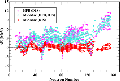
Figure 1: Residues with respect to the experimental energies of 551 spherical and deformed even-even nuclei predicted by the HFB calculation with the Gogny D1S force (magenta symbols) luis and by the Mic-Mac Gogny-based models fitted to experimental energies (red symbols) and to HFB energies (cyan symbols).

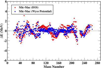
Figure 2: Residues with respect to experiment for the energies of 551 spherical and deformed even-even nuclei calculated with the WK Mic-Mac models based on the Gogny D1S force (red symbols) and on the phenomenological Wyss potential (blue symbols).

In Figure 1 we display by red symbols the residues (the differences between the calculated and experimental energies) of 551 spherical and deformed even-even nuclei, the masses of which are experimentally well determined, calculated with our Gogny-based WK Mic-Mac model. In the same figure we show with magenta symbols the residues of the HFB energies computed using the same D1S force and the same set of nuclei. As it can be seen, the pattern exhibited by the two calculations performed with the same D1S interaction is clearly different. On the one hand, the HFB energies calculated with the D1S interaction show the well-known energy drift for neutron-rich nuclei pillet17 , while in the Mic-Mac calculation, where the macroscopic part is fitted to experimental masses, this drift is completely washed out and the predictions are very similar to the ones obtained in our previous calculation bhagwat12 with the phenomenological Wyss potential, as it can be clearly appreciated in Figure 2. On the other hand, our Gogny-based Mic-Mac model is able to reproduce quite accurately the HFB results when the liquid-drop parameters of our model have been fitted to the HFB energies. This can be seen in Figure 1 where the predictions of our Mic-Mac model in this case are given by cyan symbols. The Gogny-based WK Mic-Mac model fitting the macroscopic part to the full quantal HFB energies reproduces the experimental masses of the selected set of nuclei with a similar rms deviation $\sim$4 MeV as the one provided by HFB calculation, pointing out that the Mic-Mac model is a consistent approach and captures the essential physics of the full quantal calculation.

Our results show that the energies calculated using our WK Mic-Mac model with the macroscopic part fitted to the experimental data are to some extent independent of the external potential used to determine the microscopic part. This is due to the fact that the relatively small differences in the microscopic energies computed with different external potentials can be easily absorbed by the large macroscopic part through a variation of the liquid drop parameters. In this respect, it is expected that the energies predicted by our Gogny-based model starting from a different Gogny interaction, say D1M goriely09 for example, would predict on average similar energies if the parameters of the macroscopic part are fitted to the experimental data, the differences with the results reported in this work, obtained using the D1S force, being relatively marginal.

It is well known that the D1S Gogny interaction suffers from a drift in the energy with respect to the experimental values when the number of neutrons increases for a given nucleus (see pillet17 and references therein) as can be clearly seen in Figure 1. To overcome this deficiency, new Gogny interactions of the D1 family, namely D1N chappert08 and D1M goriely09 were proposed. These interactions include in the fitting protocol of their parameters new constraints such as, among others, that of reproducing qualitatively the trends of a microscopic equation of state in neutron matter. As can be seen in Figure 1, the Mic-Mac model based on the Gogny D1S force also removes the drift in the binding energies along isotopic chains. Therefore it is expected that this Mic-Mac model can reproduce the experimental energies in heavy neutron rich nuclei better than the HFB calculations using in both cases the same D1S interaction. To analyze more in detail the differences between the full HFB and the Mic-Mac ground-state energies, we report in Table 2 the binding energies along the Pb isotopic chain computed at HFB and Mic-Mac levels. From this Table it is seen that the HFB energies in this isotopic chain exhibit a systematic behaviour with respect to the Mic-Mac Gogny results obtained in the present work. In particular, we see that for neutron-deficient Pb isotopes, both, HFB and Mic-Mac, agree well with the experiment. With increasing neutron number, the two predictions deviate from each other. The Mic-Mac results remain close to the experiment, but the HFB results deviate strongly from it. As the shell closure approaches, the Mic-Mac results start to deviate from the experiment, whereas the HFB values go on improving. Away from the shell closure, the Mic-Mac calculations again improve, whereas HFB starts deviating from experiment (²¹⁴Pb) as a consequence of the energy drift mentioned before.

Table 2: Binding energies (in MeV) for Pb isotopes. Those reported at luis and the experimental values are also quoted for comparison. Notice that the contribution to the experimental energies from electronic binding has been removed here.

$A$	This work	Ref. luis	Expt.
178	-1367.60	-1369.13	-1368.40
180	-1389.28	-1389.94	-1390.05
182	-1410.37	-1410.26	-1411.08
184	-1430.90	-1430.09	-1431.45
186	-1450.88	-1449.44	-1451.23
188	-1470.31	-1468.37	-1470.50
190	-1489.26	-1486.88	-1489.25
192	-1507.70	-1505.02	-1507.54
194	-1525.58	-1522.79	-1525.32
196	-1542.83	-1540.20	-1542.62
198	-1559.33	-1557.26	-1559.45
200	-1575.19	-1573.96	-1575.79
202	-1590.56	-1590.28	-1591.63
204	-1605.48	-1606.21	-1606.94
206	-1619.91	-1621.66	-1621.76
208	-1633.29	-1636.44	-1635.86
210	-1643.09	-1643.79	-1644.98
212	-1652.12	-1650.81	-1653.95
214	-1660.87	-1657.49	-1662.72

III.2 Comparison with other Mic-Mac models

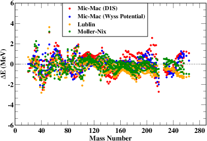
Figure 3: Residues with respect to experiment for the energies of 551 spherical and deformed even-even nuclei obtained with the Mic-Mac models FRDM moller97 , LSD pomorski03 and our WK model using the Gogny-based and the phenomenological (Wyss) potentials as external mean fields.

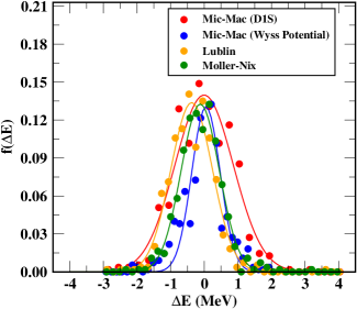
Figure 4: Binned data and the corresponding Gaussian fits for the different Mic-Mac models considered in the present study (see text for more detail).

In this subsection we want to compare the predictions of our Gogny-based Mic-Mac models with the results provided by very well-known Mic-Mac models such as the FRDM of Möller and Nix moller97 , the LSD of Pomorski and Dudek pomorski03 and the WK Mic-Mac model based on the phenomenological Wyss potential bhagwat10 ; bhagwat12 . These comparisons are performed for the chosen set of 551 spherical and deformed nuclei with well-determined masses according to the Audi 2012 evaluation audi12 . To this end, we display in Figure 3 the residues with respect to the experimental energy predicted by the FRDM, LSD, WK Wyss potential and the Gogny-based WK Mic-Mac model developed in this work. From Figure 3 we can see that, globally, all the considered Mic-Mac models are quite equivalent for describing ground-state energies with residuals that are not larger than $\pm$ 2 MeV along the whole periodic table. All the considered models show, globally, similar trends, with the largest residues corresponding to magic numbers. Another common property of these residues is the fact that they are relatively larger for low mass than for heavy mass nuclei. The fact that all these models qualitatively behave more or less alike needs a more detailed analysis. In order to do so, we have binned the residues $\Delta E=E_{cal.}-E_{expt}$, i.e. the difference between the calculated and experimental energies, in a suitable way to get the normalized frequency distribution. The bin size was chosen carefully through the well-known Freedman-Diaconis procedure freedman81 ; izenman91 . It is well known that this choice of the bin size is quite robust, and works well for a range of underlying probability distributions, so long as the probability distributions are square integrable functions.

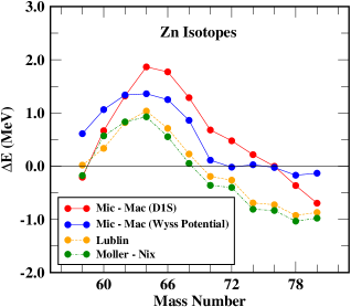
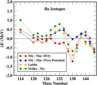
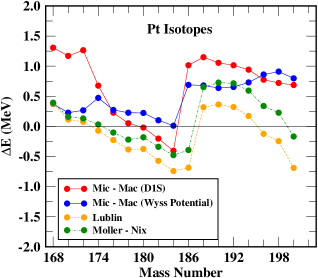
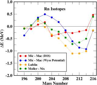
Figure 5: The difference between the calculated and the experimental audi12 energies for Zn, Ba, Pt and Rn isotopes.

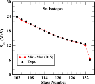
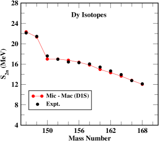
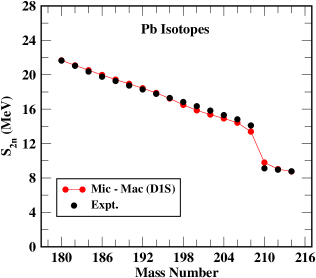
Figure 6: Calculated and experimental values of two-neutron separation energies.

The binned data plotted along with the corresponding fitted Gaussian profiles are displayed in Figure 4. We can see that all the four sets of data yield almost Gaussian profiles, with correlation coefficients greater than 0.95 in all the four cases. All the distributions have a central peak of height $\sim$0.13 at $\Delta E\sim 0$, indicating that about 13% of the data is described with deviation of $\sim 0$ with respect to the experimental data. Apart from the different standard deviations in all the four models, the profiles of the residues were found to be very similar, supporting the previous observation that all the four mass models are more or less equivalent, globally speaking. A more detailed inspection of this Figure 4 shows that our WK models are well centered around $\Delta E\sim 0$, while LSD and FRDM show a small shift towards negative $\Delta E$ values, which is more important for the LSD data. This fact indicates that on average our WK results are well scattered around the experimental energies while LSD and FRDM show a slight tendency of overbinding, at least for the considered set of nuclei. The widths of the Gaussian fits suggest that, for the considered set of nuclei, the quality of the WK results using the phenomenological Wyss potential is somewhat better than the quality of the predictions of the FRDM and LSD calculations. From this Figure it is also clear that width of the Gaussian associated to the WK Gogny-based potential calculation is larger than the other widths displayed in the Figure, pointing out that the energy description for the set of considered nuclei provided by the WK Gogny-based Mic-Mac model is a fringe worse than the one obtained using the other models considered in this analysis.

In order to investigate the predictive power of the WK Gogny-based model in different regions of the nuclear chart, we show in Figure 5 the residues with respect to the experimental values of the energies along the Zn, Ba, Pt and Rn isotopic chains computed with our Gogny-based WK model in comparison with the predictions of the FRDM, LSD and WK Wyss potential. For Zn isotopes, the FRDM and LSD predictions are somewhat better than the ones of both WK models for mass numbers between $A$=60 and $A$=70, and the opposite is true for the heaviest isotopes of the chain, where the mass numbers are in the range between $A$=74 and $A$=80. However, in general, the predictions of the WK Gogny-based model underbinds the experimental energies, mainly around $A$=60–66. For Ba isotopes, the predictions of the FRDM, LSD and both WK models agree reasonably well except, may be, around the magic neutron number $N$=82 (corresponding to ¹³⁸Ba) where the Gogny-based WK calculation predicts larger differences with respect to the experiment than the FRDM, LSD and WK Wyss models. For Pt isotopes, the FRDM, LSD and both WK residues show, qualitatively, a similar behaviour. However, in general, the residues corresponding to the WK Gogny-based model are larger than the ones predicted by the FRDM, LSD and WK Wyss calculations. For Rn isotopes, the WK Gogny-based model predicts similar binding energies than the other Mic-Mac models considered in the range of mass numbers between $A$=196 and $A$=206, while in the intermediate region with mass numbers between $A$=208 and $A$=210, the residues predicted by the WK Gogny-based model are a bit smaller than the ones found in the FRDM, LSD and WK Wyss calculations. Let us mention that the good agreement between the residues obtained in the FRDM and LSD calculations is, actually, due to the fact that both models use the same microscopic part.

A more quantitative information about the goodness of the different Mic-Mac models analyzed in this work is provided by the energy rms deviations, which for the set of considered nuclei are 635 keV (FRDM), 731 keV (LSD), 609 keV WK(Wyss) and 834 keV WK(Gogny). The fact that the rms deviation predicted by our WK Gogny-based calculation (834 keV) is larger than the one obtained with our WK method using the phenomenological Wyss potential (609 keV), which in turn is similar to the rms deviation corresponding to FRDM and LSD models for the same set of nuclei, can be appreciated in Figure 2. In this figure we can see that the prediction of the WK model based on the Wyss potential gives a better description of the experimental energies in the range between $A\sim$100 and $A\sim$200 than the WK Gogny-based calculation. These facts show the limits of the predictive power of the Mic-Mac model based on the D1S interaction and suggest the two following comments. On the one hand, the use of a more accurate Gogny interaction for describing finite nuclei, as for example D1M goriely09 , which is free of the energy drift discussed before, may slightly improve the quality of the description of ground-state energies with the WK Gogny-based model. Although the global quality of the WK Gogny-based model is lower by a very small amount for describing ground-state energies as compared with the predictions of the other Mic-Mac models considered in this work, it is accurate enough to give predictions in good agreement with the experimental data. As an example, we display the two-neutron separation energies for Sn, Dy and Pb isotopes in Figure 6. The excellent agreement between calculations and experiment can be clearly seen in the figure. However, despite the globally good performance, we must admit that the use of a more microscopically based mean field as the one used here, which is based on the Gogny D1S force, does not show any decisive advantage over, e.g, the purely phenomenological Wyss potential, in what concerns the calculation of nuclear masses.

However, some remarks on the underlying physics of our Mic-Mac approach are in order. The Gogny D1S Mic-Mac results clearly show that the relatively large rms deviation of 3.95 MeV (see Table 1) of the microscopic HFB D1S masses is not necessarily to be incriminated to a bad behavior of the shell structure (given by the shell correction energies) but rather due to a deficiency of the bulk behavior. It is most obvious that the LDM part of our Mic-Mac model saves the bulk part from the neutron drift. But even if we take a Gogny version which is free from the drift, as for instance D1M, for which the rms deviation is 1.34 MeV, our Mic-Mac model for the considered nuclei still performs essentially better (as a reminder the rms deviation is 0.834 MeV in our model), as it can also be seen seen from Figure 7 where the residuals obtained from the D1M HFB calculation and from our Mic-Mac model are plotted as a function of the neutron number. This suggests that, in general, a HFB calculation with effective Gogny forces cannot reproduce at the same time good bulk and good shell effects behavior. This fact is clear for the calculation with the D1S interaction, but can also be appreciated in the case of the D1M force as just explained. Actually it can be concluded that it is the bulk part of the HFB energy computed with the Gogny force which is deficient and can be improved by the LDM contribution. For example the difficulty for evaluating the zero point motion contribution is automatically included in the LDM part. This conclusion is in fact quite general and it arises from the lack of flexibility of the effective interaction, where both microscopic and macroscopic parts are coupled. It is by means of a highly sophisticated functional with 30 parameters including an additional Mac part (Wigner term) that the semi-microscopic HFB model of the Brussels group goriely13 yields simultaneously good bulk and good shell structure. In our opinion, there is a room for for further improvement in the Mic-Macmodels. This concerns not so much the LDM part, which we think is determined in a quite optimal way, as the shell correction part with, for instance, its behaviour around magic and doubly magic nuclei. It is one of our objectives to work on this in the future.

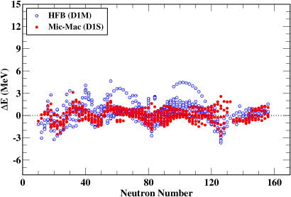
Figure 7: Residues with respect to experiment for the energies of 551 spherical and deformed even-even nuclei calculated with the WK Mic-Mac model based on the Gogny D1S force (filled red symbols) and the HFB results calculated with the Gogny D1M force (open blue symbols).

           

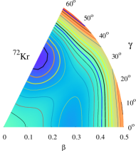
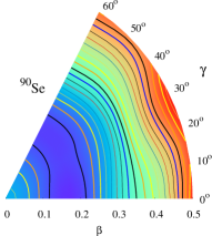
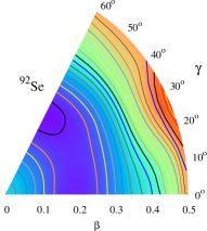
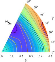
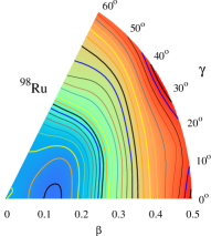
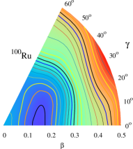
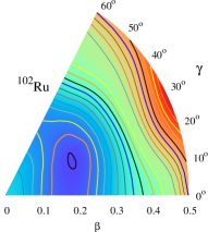
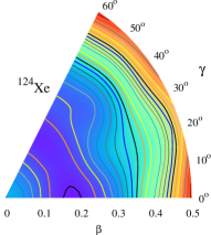
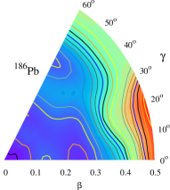
Figure 8: Potential energy surfaces for a set of nuclei spanning almost the entire periodic table. See text for details.

IV Potential Energy Surfaces

The potential energy surfaces (PES) have been generated by suitably transforming the binding energies into Cartesian representation. Considering the fact that the maxima and the minima differ by at the most 10 MeV in our present set of nuclei, the sampling has been done with a bin size of 0.4 MeV.

As representative cases, we plot the potential energy surfaces for ⁷²Kr, ^90,92,94Se, ^98,100,102Ru, ¹²⁴Xe and ¹⁸⁶Pb. These have been so chosen as to demonstrate existence of well-defined minima (prolate or oblate), the shape-coexistence phenomenon, as well as $\gamma$-softness.

As expected, ⁷²Kr turns out to be very well defined oblate, with deformation parameter ($\beta_{2}$) of the order of 0.3. This is in agreement with the other Mic-Mac calculations, such as Möller-Nix and our calculation with Wyss potential. The ⁷²Kr nucleus turns out to have a second prolate minimum at $\beta_{2}\sim 0.275$ around 1.5 MeV away from the deepest minimum. This topography is at variance with that predicted by the pure HFB calculation with the D1S force, which predicts the existence of two closely spaced minima in the oblate region hilaire08 .

The three Selenium isotopes exhibit the shape coexistence phenomenon. In particular, the ground state of the nucleus ⁹⁰Se is predicted to be prolate with $\beta_{2}\sim 0.175$, possesses a second minimum for oblate $\beta_{2}\sim 0.2$, with a difference between the two of the order of just 200 keV. On the other hand, ^92,94Se are predicted to have oblate minima, with the second minima (prolate) which are $\sim$200 keV and $\sim$600 keV away respectively. Further, the potential energy surface as a function of $\gamma$ for $\beta_{2}$ around 0.2 turns out to be quite flat, particularly for ⁹⁰Se, indicating a possible existence of $\gamma$-softness. These observations are similar to that reported in Ref. nomura17 . Out of the three Ruthenium isotopes, ^98,100Ru are strongly prolate, with a rather flat PES for $\gamma$ up to 20^∘. The nucleus ¹⁰²Ru turns out to be $\gamma$-soft, with a triaxial minimum appearing for $\beta_{2}\sim 0.2$ and $\gamma\sim 20^{\circ}$, which is in agreement with the Möller-Nix predictions.

The nucleus ¹²⁴Xe possesses a prolate minimum ($\beta_{2}\sim 0.2$) and the second minimum is oblate which is about 400 keV away from the deepest minimum. Interestingly, the PES for this nucleus turns out to be quite flat as a function of $\gamma$, for $\beta_{2}$ values around 0.2, hinting towards a possible existence of $\gamma$-softness. Notice that this behaviour is similar to that observed for Selenium isotopes. The nucleus ¹⁸⁶Pb turns out to have a very rich structure in its PES. The minimum in this case is spherical as expected, but there are also several possible deformed solutions within $\sim$ 400 keV of the lowest solution. From the plot of the PES it can be seen that there is a well-defined prolate minimum at $\beta_{2}\sim$ 0.25 and two rather well-defined oblate minima, one at $\beta_{2}\sim$ 0.30 and the other one at $\beta_{2}\sim$ 0.10, which is located in a very small contour line along the oblate axis. This pattern for the PES of the nucleus ¹⁸⁶Pb is in agreement with the results reported by Möller et al. moller2008 .

V Summary and Conclusions

In this paper we used mean field potentials which have been derived via the semiclassical ETF method, including $\hbar^{2}$ corrections, from the Gogny-HF approach using the D1S force. The semiclassical mean-fields are local with the effective mass incorporated into the potentials soubbotin00 . This choice was dictated by the numerics. Using those mean-field potentials in a one-shot diagonalization (the so-called expectation-value method brack85 ; bohigas76 ) allows one to recover very accurately the fully microscopic results (see Paper I bhagwat20 ). In this work, we therefore tried to combine the Mic-Mac approach and the microscopic HFB method with the Gogny force. We, thus, have firstly taken the Liquid Drop Model for the smooth part of the energy, whose parameters are fitted to the experimental masses, plus second the shell correction part obtained with our semiclassical Gogny-adopted mean field potentials. This then constitutes a Mic-Mac approach where only the shell corrections are directly connected to the parameters of the Gogny force (D1S in the present case). Not astonishingly the neutron drift of the binding energies inherent to HFB calculations with the D1S force has been eliminated while the shell effects are reproduced very accurately. The Mic-Mac calculations performed in this way are found to yield a reasonably good description of ground-state binding energies for the nuclei spanning the entire periodic table. The rms-value for binding energies obtained in this way is 834 keV. This is a value only very little worse than the ones obtained with the completely phenomenological mean field potential of, e.g., Wyss bhagwat10 for the shell effects. The present Mic-Mac calculations tend to perform well in the regions away from shell closures, whereas the HFB-Gogny results are found to be better near the shell closures. One of the main conclusions of this work is that phenomenological effective forces, like the Gogny or Skyrme forces with a limited number of adjustable parameters (around 10) are not able to yield optimal values for the macroscopic part of the energy and, at the same time, the shell model contribution. On the contrary, we think that a direct fit of the macroscopic part, via a Liquid Drop model, can optimise the smoothly varying macroscopic part of the energies bringing it very close to its exact value. This can also be seen in Fig. 7 where the average of the remaining fluctuations practically adds up to zero. For example, in this way the average of the zero poin the smoothly varying macroscopic part of the energies. For example in this way the zero point fluctuations are taken care of automatically while in a pure HFB approach they are difficult to calculate and in most HFB approaches they are not determined unambiguously. The shell effects can then be added additionally and their theoretical evaluation becomes a separate treatment making the whole approach more flexible. Since the shell energies are obtained from the difference between a semiclassical and a quantal calculation, errors may cancel out. Nonetheless, there may be more room for improvements in the shell corrections than in the LDM part. For example, it has been conjectured that the spin-orbit potential may be responsible for persisting oscillations in the differences between theoretical and experimental values. Further investigations along these lines are in progress. Let us also point out that our Mic-Mac method based on a effective two-body force performs practically as well as the most efficient Mic-Mac models on the market in order to describe ground-state properties. Only the mean field HFB approach by the Brussels group can compete with this (actually with a slightly better result) at the price to adjust around 30 parameters and still employ a macroscopic piece (the Wigner energy) on top of it. Finally, let us mention that the results reported in this work concern ground-state energies only and in order to apply this Mic-Mac method to other scenarios where large deformations are needed, such as the description of fission phenomena, would require to modify the distance function used here. Work in this direction is in progress.

Appendix 1: Order by Order Contributions to WK Energy

The WK particle number $N$ and energy can be calculated directly by Laplace inversion as

$$N~{}=~{}{\cal{L}}^{-1}_{\lambda}\left(\frac{Z_{\rm WK}^{(4)}(\beta)}{\beta}\right)$$ (17)

and

$$E_{\rm WK}~{}=~{}\lambda N~{}-~{}{\cal{L}}^{-1}_{\lambda}\left(\frac{Z_{\rm WK}^{(4)}(\beta)}{\beta^{2}}\right),$$ (18)

where $\lambda$ is the chemical potential, determined to ensure the correct particle number, $Z_{\rm WK}^{(4)}$ is the WK partition function up to $\hbar^{4}$-order, and ${\cal{L}}^{-1}_{\lambda}$ denotes the Laplace inversion. These Laplace inversions can be performed analytically.

Let $g_{\rm WK}$ be semi-classical level density (up to $\hbar^{4}$ order, in the present context), and $\lambda$ be the chemical potential as defined above. In terms of these quantities, particle number can be expressed as

$$N~{}=~{}\int_{0}^{\lambda}\,g_{WK}\left(\epsilon\right)\,d\epsilon\,.$$ (19)

This expression can be though of as a convolution of $g_{WK}$ and the Heaviside step function ($u$). Since $Z_{\rm WK}^{(4)}$ is the Laplace transform of $g_{\rm WK}$, the Laplace transform of convolution of $g_{\rm WK}$ and $u$ is $Z_{\rm WK}^{(4)}\left(\beta\right)/\beta$, which directly yields Eq. (17).

On the other hand, the averaged energy ($E_{\rm WK}$) can be expressed in terms of $g_{\rm WK}$ as:

$$E_{\rm WK}~{}=~{}\int_{0}^{\lambda}\,g_{\rm WK}\left(\epsilon\right)\epsilon\,d\epsilon\,.$$ (20)

Integrating by parts one gets:

$$E_{\rm WK} = \lambda N-\int_{0}^{\lambda}\int^{\epsilon}g_{\rm WK}\left(\varepsilon\right)\,d\varepsilon\,d\epsilon\,.$$ (21)

Notice that the second term on the right hand side of Eq. (21) can be thought of as convolution of $u$ with the convolution of $u$ and $g_{\rm WK}$. Therefore, Laplace transform of this quantity is $Z_{\rm WK}^{(4)}\left(\beta\right)/\beta^{2}$, which automatically leads to Eq. (18).

The explicit expressions of the energy, which are used in Eq. (LABEL:EJEN) of the main text, are as follows (see bhagwat10 for further details):

$$E_{\hbar^{0}}^{\rm CN} = \frac{1}{3\pi^{2}}\left(\frac{2m}{\hbar^{2}}\right)^{3/2}\int d\vec{r}\left\{\frac{2}{5}\left(\lambda-V\right)^{5/2}\right\}\Theta\left(\lambda-V\right)$$ (22)

$$E_{\hbar^{2}}^{\rm CN} = -\frac{1}{24\pi^{2}}\left(\frac{2m}{\hbar^{2}}\right)^{1/2}\int d\vec{r}\left\{\left(\lambda-V\right)^{1/2}\nabla^{2}V\right\}\Theta\left(\lambda-V\right)$$ (23)

$$E_{\hbar^{4}}^{\rm CN} = -\frac{1}{5760\pi^{2}}\left(\frac{\hbar^{2}}{2m}\right)^{1/2}\left[\int d\vec{r}\left(\lambda-V\right)^{-1/2}\left\{7\nabla^{4}V\right\}\Theta\left(\lambda-V\right)\right.$$ (24)

$$\left.\hskip 85.35826pt+\frac{1}{2}\int d\vec{r}\left(\lambda-V\right)^{-3/2}\left\{5\left(\nabla^{2}V\right)^{2}+\nabla^{2}\left(\nabla V\right)^{2}\right\}\Theta\left(\lambda-V\right)\right]$$

$$E_{\hbar^{2}}^{\rm SO} = \frac{\kappa^{2}}{6\pi^{2}}\left(\frac{2m}{\hbar^{2}}\right)^{1/2}\int d\vec{r}\left\{\left(\lambda-V\right)^{3/2}\left(\nabla f\right)^{2}\right\}\Theta\left(\lambda-V\right)$$ (25)

$$E_{\hbar^{4}}^{\rm SO} = \frac{1}{48\pi^{2}}\left(\frac{\hbar^{2}}{2m}\right)^{1/2}\int d\vec{r}\left(\lambda-V\right)^{1/2}\left[\kappa^{2}\left\{\frac{1}{2}\nabla^{2}\left(\nabla f\right)^{2}-\left(\nabla^{2}f\right)^{2}+\nabla f\cdot\nabla\left(\nabla^{2}f\right)\right.\right.$$

$$\left.\left.-\frac{\left(\nabla f\right)^{2}\nabla^{2}V}{2\left(\lambda-V\right)}\right\}-2\kappa^{3}\left\{\left(\nabla f\right)^{2}\nabla^{2}f-\frac{1}{2}\nabla f\cdot\nabla\left(\nabla f\right)^{2}\right\}+2\kappa^{4}\left(\nabla f\right)^{4}\right]\Theta\left(\lambda-V\right),$$

where CN and SO refer to the contributions arising from the central and spin-orbit parts of the partition function, $\kappa$ is the strength of the spin-orbit interaction, and $f$ is the spin-orbit form factor. In the present work the potentials appearing in the above expressions as well as the spin-orbit form factor are of the generalized Woods - Saxon form. The explicit expressions of the derivatives of the generalized Woods - Saxon function have been listed in Appendix - 2.

We shall now demonstrate that the semi - classical energy, as written above, reduces to the well known Thomas Fermi form. In order to do so, first, notice that the chemical potential $\lambda$ here is obtained by demanding the correct particle number. The particle number, in turn is obtained by integrating the semi-classical density, which needs to be expanded only to the second order in $\hbar$ so that the energy is correct up to the fourth order in $\hbar$ (see, for example, jennings75 ). If $\rho_{\rm WK}$ is the semi-classical density, we can write:

$$\lambda N = \int d\vec{r}\,\left\{\vphantom{\frac{1}{1}}\lambda\rho_{\rm WK}\right\}\Theta\left(\lambda-V\right)$$

$$= \int d\vec{r}\,\left\{\vphantom{\frac{1}{1}}\left(\lambda-V\right)\rho_{\rm WK}\right\}\Theta\left(\lambda-V\right)$$

$$+ \int d\vec{r}\,\left\{\vphantom{\frac{1}{1}}\rho_{\rm WK}\,V\right\}\Theta\left(\lambda-V\right)$$

Up to leading order, $\rho_{\rm WK}$ is given by:

$$\rho_{\rm WK} = \frac{1}{3\pi^{2}}\left(\frac{2m}{\hbar^{2}}\right)^{3/2}\left(\lambda-V\right)^{3/2}\Theta\left(\lambda-V\right)$$ (27)

Using this expression in the expression for $\lambda N$ above, we get:

$$\lambda N = \frac{1}{3\pi^{2}}\left(\frac{2m}{\hbar^{2}}\right)^{3/2}\int d\vec{r}\,\left\{\left(\lambda-V\right)^{5/2}\right\}\Theta\left(\lambda-V\right)$$

$$+ \frac{1}{3\pi^{2}}\left(\frac{2m}{\hbar^{2}}\right)^{3/2}\int d\vec{r}\,\left\{V\left(\lambda-V\right)^{3/2}\right\}\Theta\left(\lambda-V\right)$$

up to leading order. This expression, when combined with that for $E_{\hbar^{0}}^{CN}$, yields:

$$E_{TF} = \frac{1}{3\pi^{2}}\left(\frac{2m}{\hbar^{2}}\right)^{3/2}\int d\vec{r}\,\left\{\frac{3}{5}\left(\lambda-V\right)^{5/2}\right\}\Theta\left(\lambda-V\right)$$

$$+ \frac{1}{3\pi^{2}}\left(\frac{2m}{\hbar^{2}}\right)^{3/2}\int d\vec{r}\,\left\{V\left(\lambda-V\right)^{3/2}\right\}\Theta\left(\lambda-V\right)$$

On the right hand side of $E_{TF}$, the first term corresponds to the kinetic energy and the second to the potential energy within the Thomas Fermi approximation. Proceeding along the same lines, we get the usual expressions (see, for example, brack97 ) for second order corrections to kinetic and potential energies (excluding the spin-orbit contributions):

$$E_{\hbar^{2}}^{\rm KE} = \frac{1}{24\pi^{2}}\left(\frac{2m}{\hbar^{2}}\right)^{1/2}\int d\vec{r}\left\{\vphantom{\frac{x^{5}}{x^{5}}}\left(\lambda-V\right)^{1/2}\nabla^{2}V\right.$$ (30)

$$\left.-\frac{3}{4}\frac{\left(\nabla V\right)^{2}}{\left(\lambda-V\right)^{1/2}}\right\}\Theta\left(\lambda-V\right)$$

$$E_{\hbar^{2}}^{\rm PE} = \frac{-1}{24\pi^{2}}\left(\frac{2m}{\hbar^{2}}\right)^{1/2}\int d\vec{r}\left\{\frac{V\nabla^{2}V}{\left(\lambda-V\right)^{1/2}}\right.$$ (31)

$$\left.+\frac{1}{4}\frac{V\left(\nabla V\right)^{2}}{\left(\lambda-V\right)^{3/2}}\right\}\Theta\left(\lambda-V\right)$$

Appendix 2: Explicit Formulas for Derivatives of Modified Woods - Saxon Form Factor

Here we list the explicit formulas for derivatives of Woods - Saxon form factor. Let

$$g(r)=\Bigl{[}g_{0}\left(\vec{r}\right)\Bigr{]}^{\gamma}$$ (32)

with $\gamma>0$ and

$$g_{0}\left(\vec{r}\right)=\frac{1}{1+\exp\left(l\left(\vec{r}\right)/a\right)}$$ (33)

with $l\left(\vec{r}\right)$ is suitably defined distance function (see, for example, bhagwat10 ) and $a$ is the diffusivity parameter. We shall henceforth suppress all the arguments of the functions for the sake of brevity. Define:

$$\xi = g\left(g_{0}-1\right)$$ (34)

$$\xi_{0} = g_{0}\left(g_{0}-1\right)$$ (35)

$$\zeta = \left(\gamma+1\right)g_{0}-\gamma$$ (36)

Evaluation of the different contributions to the semi - classical energy requires gradient of $g$ as well as derivatives of $\left(\nabla g\right)^{2}$. These are listed below first. We have:

$$\nabla g=\frac{\gamma}{a}\,\xi\nabla l$$ (37)

giving us,

$$\left(\nabla g\right)^{2} = \frac{\gamma^{2}}{a^{2}}\,\xi^{2}\left(\nabla l\right)^{2}$$ (38)

$$\nabla\left(\nabla g\right)^{2} = \frac{\gamma^{2}}{a^{2}}\,\xi^{2}\left[\nabla\left(\nabla l\right)^{2}+\frac{2}{a}\,\zeta\left(\nabla l\right)^{2}\nabla l\right]$$ (39)

$$\nabla^{2}\left(\nabla g\right)^{2} = \frac{2\gamma^{2}}{a^{3}}\,\xi^{2}\,\zeta\left[\nabla l\cdot\nabla\left(\nabla l\right)^{2}+\frac{2}{a}\,\zeta\left(\nabla l\right)^{4}\right]+\frac{\gamma^{2}}{a^{2}}\,\xi^{2}\left[\nabla^{2}\left(\nabla l\right)^{2}+\frac{2}{a}\,\zeta\left\{\nabla^{2}l\left(\nabla l\right)^{2}+\nabla l\cdot\nabla\left(\nabla l\right)^{2}\right\}\right.$$ (40)

$$\left.+\frac{2}{a^{2}}\left(\gamma+1\right)\xi_{0}\left(\nabla l\right)^{4}\right]$$

In addition to these, the expressions for different terms appearing in the semi - classical energy requires Laplacian of $g$ as well as derivatives of $\nabla^{2}g$. These can be expressed as:

$$\nabla^{2}g = \frac{\gamma}{a}\,\xi\left[\nabla^{2}l+\frac{1}{a}\,\zeta\left(\nabla l\right)^{2}\right]$$ (41)

$$\nabla\left(\nabla^{2}g\right) = \frac{\gamma}{a^{2}}\,\xi\,\zeta\left[\nabla^{2}l+\frac{1}{a}\,\zeta\left(\nabla l\right)^{2}\right]\nabla l+\frac{\gamma}{a}\,\xi\left[\vphantom{\frac{1}{1}}\nabla\left(\nabla^{2}l\right)+\frac{1}{a^{2}}\left(\gamma+1\right)\xi_{0}\left(\nabla l\right)^{2}\nabla l+\frac{1}{a}\,\zeta\nabla\left(\nabla l\right)^{2}\right]$$ (42)

$$\nabla^{2}\left(\nabla^{2}g\right) = \frac{\gamma}{a^{2}}\,\xi\,\zeta\left[\nabla^{2}l+\frac{1}{a}\,\zeta\left(\nabla l\right)^{2}\right]\nabla^{2}l+\frac{2\gamma}{a^{2}}\,\xi\,\zeta\left[\nabla l\cdot\nabla\left(\nabla^{2}l\right)+\frac{1}{a}\,\zeta\nabla l\cdot\nabla\left(\nabla l\right)^{2}+\frac{1}{a^{2}}\left(\gamma+1\right)\xi_{0}\left(\nabla l\right)^{4}\right]$$ (43)

$$+ \frac{\gamma}{a^{3}}\,\xi\left(\nabla l\right)^{2}\left\{\vphantom{\frac{1}{1}}\zeta^{2}+\left(\gamma+1\right)\xi_{0}\right\}\left[\nabla^{2}l+\frac{1}{a}\,\zeta\left(\nabla l\right)^{2}\right]+\frac{\gamma}{a}\,\xi\left[\nabla^{2}\left(\nabla^{2}l\right)+\frac{1}{a^{3}}\left(\gamma+1\right)\left(2g_{0}-1\right)\xi_{0}\left(\nabla l\right)^{4}\right.$$

$$\left.+\frac{1}{a^{2}}\left(\gamma+1\right)\xi_{0}\left(\left(\nabla l\right)^{2}\nabla^{2}l+2\nabla l\cdot\nabla\left(\nabla l\right)^{2}\right)+\frac{1}{a}\,\zeta\nabla^{2}\left(\nabla l\right)^{2}\right]$$

The derivatives of distance function are not presented here, since the details would depend on the particular choice of distance function. In the present context, we are assuming reflectionally symmetric shapes. Therefore, it is most convenient to work in spherical polar system, as explained in bhagwat10 . In this case, spherical harmonics appearing in the distance function can be suitably combined to write $R_{s}$ (see Eq. (6)) in terms of multiple angle formulas of the trigonometric functions, which makes explicit evaluation of the derivatives relatively easier.

- (1) A. Bhagwat, M. Centelles, X. Viñas, and P. Schuck, “Woods-Saxon-type of mean-field potentials with effective mass derived from the D1S Gogny force”, submitted to Phys. Rev. C (2020).
- (2) G. Audi, M. Wang, A. H. Wapstra, F. G. Kondev, M. MacCormick, X. Xu and B. Pfeiffer, Chin. Phys. C 36, 1287 (2012).
- (3) D. Vautherin and D. M. Brink, Phys. Rev. C 5, 626 (1972).
- (4) Li Guo-Qiang, J. Phys. G: Nucl. Part. Phys. 17, 1 (1991).
- (5) E. Chabanat, P. Bonche, P. Haensel, J. Meyer and R. Schaeffer, Nucl. Phys. A 635, 231 (1998).
- (6) J. R. Stone and P.-G. Reinhard, Prog. Part. Nucl. Phys. 58, 587 (2007).
- (7) J. Dechargé and D. Gogny, Phys. Rev. C 21, 1568 (1980).
- (8) J. F. Berger, M. Girod and D. Gogny, Comp. Phys. Commun. 63, 365 (1991).
- (9) F. Chappert, M. Girod and S. Hilaire, Phys. Lett. B 668, 420 (2008).
- (10) S. Goriely, S. Hilaire, M. Girod and S. Péru, Phys. Rev. Lett. 102, 242501 (2009).
- (11) B. Behera, X. Viñas, T.S. Routray, L. M. Robledo, M. Centelles and S. P. Pattnaik, J. Phys. G: Nucl. Part. Phys. 43, 045115 (2016).
- (12) H. Nakada, Phys. Rev. C 68, 014316 (2003); Phys. Rev. C 78, 054301 (2008); Phys. Rev. C 81, 027301 (2010).
- (13) M. Baldo, L. M. Robledo, P. Schuck and X. Viñas, Phys. Rev. C 87, 064305 (2013).
- (14) M. Baldo, L. M. Robledo, P. Schuck and X. Viñas, Phys. Rev. C 95, 014318 (2017).
- (15) D. Vretenar, A. V. Afanasjev, G. A. Lalazissis and P. Ring, Phys. Rep. 409, 101 (2005).
- (16) P. Ring and P. Schuck, The Nuclear Many-Body Problem (Springer-Verlag, Berlin, 1980).
- (17) S. Goriely, N. Chamel and J. M. Pearson, Phys. Rev. Lett. 102, 152503 (2009).
- (18) S. Goriely, N. Chamel and J. M. Pearson, Phys. Rev. C 88, 024308 (2013).
- (19) M. Kortelainen, J. McDonnell, W. Nazarewicz, E. Olsen, P.-G. Reinhard, J. Sarich, N. Schunck, S. M. Wild, D. Davesne, J. Erler and A. Pastore Phys. Rev. C 89, 054314 (2014).
- (20) AMEDEE database, DOI:10.105/ndata:07709.
- (21) P. Möller, J. R. Nix, W. D. Myers and W. J. Swiatecki, Atom. Data Nucl. Data Tables 59, 185 (1995).
- (22) P. Möller, J. R. Nix and K. -L. Kratz, Atom. Data Nucl. Data Tables 66, 131 (1997).
- (23) K. Pomorski and J. Dudek, Phys. Rev. C 67, 044316 (2003).
- (24) W. D. Myers and W. J. Swiatecki, Ann. Phys. (N.Y.) 55, 395 (1969); Ann. Phys. (N.Y.) 84, 186 (1974).
- (25) A. Bhagwat, X. Viñas, M. Centelles, P. Schuck and R. Wyss, Phys. Rev. C 81, 044321 (2010).
- (26) A. Bhagwat, X. Viñas, M. Centelles, P. Schuck and R. Wyss, Phys. Rev. C 86, 044316 (2012).
- (27) V. M. Strutisnky, Nucl. Phys. A 95, 420 (1967).
- (28) G. G. Bunatian, V. M. Kolomietz and V.M . Strutinsky Nucl. Phys. A 188, 225 (1972).
- (29) M. Kleban, B. Nerlo-Pomorska, J. F. Berger, J. Dechargé, M. Girod and S. Hilaire, Phys. Rev. C 65, 024309 (2002).
- (30) Y. H. Chu, B. K. Jennings and M. Brack, Phys. Lett. B 68, 407 (1977).
- (31) A. K. Dutta, J.-P. Arcoragi, J. M. Pearson, R. Behrman and F. Tondeur, Nucl. Phys. A 458, 77 (1986).
- (32) F. Tondeur, A. K. Dutta, J. M. Pearson and R. Behrman, Nucl. Phys. A 470, 93 (1987).
- (33) J.M. Pearson, Y. Aboussir, A. K. Dutta, R,C, Nayak, M. Farine and F. Tondeur, Nucl. Phys. A 528, 1 (1991).
- (34) Y. Aboussir, Y. Aboussir, A. K. Dutta and F. Tondeur, Nucl. Phys. A 549, 155 (1991).
- (35) Y. Aboussir, J.M. Pearson, A. K. Dutta and F. Tondeur, At. Data. Nucl. Data Tables 61, 127 (1995).
- (36) F. Tondeur, S. Goriely, J.M. Pearson and M. Onsi, Phys. Rev. C 62, 024308 (2000).
- (37) A. Mamdouh, J.M. Pearson, M. Rayet and F. Tondeur, Nucl. Phys. A 679, 337 (2001).
- (38) J. M. Pearson, N. Chamel, A. Y. Potekhin, A. F. Fantina, C. Ducoin, A. K. Dutta and S. Goriely, Mon. Not. R. Astron. Soc. 481, 2994 (2018).
- (39) C. Mondal, X. Viñas, M. Centelles and J. N. De, Phys. Rev. C 102, 015802 (2020).
- (40) E. Wigner, Phys. Rev. 40, 749 (1932).
- (41) J. G. Kirkwood, Phys. Rev. 44, 31 (1933).
- (42) B. K. Jennings, R. K. Bhaduri and M. Brack, Nucl. Phys. A 253, 29 (1975).
- (43) M. Brack, C. Guet and H. -B. Håkansson, Phys. Rep. 123, 275 (1985).
- (44) M. Brack and R. K. Bhaduri, Semiclassical Physics (Addison-Wesley Publishing Co., 1997).
- (45) M. Centelles, P. Leboeuf, A. G. Monastra, J. Roccia, P. Schuck and X. Viñas, Phys. Rev. C 74, 034332 (2006).
- (46) M. Centelles, P. Schuck and X. Viñas, Ann. Phys. (N.Y.) 322, 363 (2007).
- (47) B. Mohammed-Azizi and D. E. Medjadi, Phys. Rev. C 74, 054302 (2006).
- (48) S. Shlomo, Nucl. Phys. A 539, 17 (1992).
- (49) O. Bohigas, X. Campi, H. Krivine and J. Treiner, Phys. Lett. B 64, 381 (1976).
- (50) M. Centelles, X. Viñas, M. Barranco and P. Schuck, Nucl. Phys. A 519, 73 (1990).
- (51) M. Centelles, X. Viñas, M. Barranco and P. Schuck, Ann. Phys. (NY) 221, 165 (1993).
- (52) V. B. Soubbotin and X. Viñas, Nucl. Phys. A 665, 291 (2000).
- (53) K. A. Gridnev, V. B. Soubbotin, X. Viñas and M. Centelles, Quantum Theory in honour of Vladimir A. Fock, Y. Novozhilov and V. Novozhilov (Eds.) Publishing Group of MicMac-p2-Dec26.tex St.Petersburg University 1998, p.118; arXiv 1704.03858.
- (54) V. B. Soubbotin, V. I. Tselyaev and X. Viñas, Phys. Rev. C 67, 014324 (2003).
- (55) W. D. Myers and W. J. Swiatecki, Nucl. Phys. A 81,1 (1966).
- (56) N. Pillet and S. Hilaire, Eur. Phys. J. A 53, 193 (2017).
- (57) L. M. Robledo, HFBaxial computer code (2002).
- (58) D. Freedman and P. Diaconis, Z. Wahrscheinlichkeitstheorie verw. Gebiete 57, 453 (1981).
- (59) A. J. Izenman, J. Am. Stat. Assoc. 86, 205 (1991).
- (60) K. Nomura, R. Rodríguez-Guzmán and L. M. Robledo, Phys. Rev. C 95, 064310 (2017).
- (61) P. Möller, R. Bengstsson, B. G. Carlsson, P. Olivius, T. Ichikawa, H. Sagawa and A. Iwamoto, At. Data Nucl. Data Tables 94, 758 (2008).
- (62) See Supplemental Material at [URL will be inserted by publisher] for the tabulated energies (calculated and experimental) of the 551 nuclei considered in this work.