Fast WordPiece Tokenization

Abstract

Tokenization is a fundamental preprocessing step for almost all NLP tasks. In this paper, we propose efficient algorithms for the WordPiece tokenization used in BERT, from single-word tokenization to general text (e.g., sentence) tokenization. When tokenizing a single word, WordPiece uses a longest-match-first strategy, known as maximum matching. The best known algorithms so far are $O(n^{2})$ (where $n$ is the input length) or $O(nm)$ (where $m$ is the maximum vocabulary token length). We propose a novel algorithm whose tokenization complexity is strictly $O(n)$. Our method is inspired by the Aho-Corasick algorithm. We introduce additional linkages on top of the trie built from the vocabulary, allowing smart transitions when the trie matching cannot continue. For general text, we further propose an algorithm that combines pre-tokenization (splitting the text into words) and our linear-time WordPiece method into a single pass. Experimental results show that our method is 8.2x faster than HuggingFace Tokenizers and 5.1x faster than TensorFlow Text on average for general text tokenization.

1 Introduction

Tokenization is the process of splitting text into smaller units called tokens (e.g., words). It is a fundamental preprocessing step for almost all NLP applications: sentiment analysis, question answering, machine translation, information retrieval, etc.

Modern NLP models like BERT Devlin et al. (2019), GPT-3 Brown et al. (2020), and XLNet Yang et al. (2019) tokenize text into subword units Schuster and Nakajima (2012); Sennrich et al. (2016); Kudo (2018). As a midpoint between words and characters, subword units retain linguistic meaning (like morphemes), while alleviating out-of-vocabulary situations even with a relatively small-size vocabulary.

In this paper, we propose efficient algorithms for WordPiece, the subword tokenization used in BERT Devlin et al. (2019). Given Unicode text that has already been cleaned up and normalized, WordPiece has two steps: (1) pre-tokenize the text into words (by splitting on punctuation and whitespaces), and (2) tokenize each word into wordpieces.

For single-word tokenization, WordPiece uses a greedy longest-match-first strategy: iteratively pick the longest prefix of the remaining text that matches a vocabulary token. This is well-known as Maximum Matching or MaxMatch Palmer (2000), which has also been used for Chinese word segmentation since 1980s Liu and Liang (1986).

Despite its wide use in NLP for decades, to the best of our knowledge, the most efficient MaxMatch algorithms so far are $O(n^{2})$ (where $n$ is the input word length) or $O(nm)$ (where $m$ is the maximum vocabulary token length) (see Section 2). It’s worth noting that the latter has a vocabulary-specific multiplicative factor $m$, which can be large when the vocabulary contains long words.

We propose LinMaxMatch, a novel MaxMatch algorithm for WordPiece tokenization, whose tokenization time is strictly $O(n)$ without any vocabulary-specific multiplicative factors. Inspired by the Aho-Corasick algorithm Aho and Corasick (1975), we organize vocabulary tokens in a trie Fredkin (1960) and introduce precomputed failure links and failure pops. During tokenization, if an input character does not match any trie edge, we perform smart transitions to avoid backtracking to earlier input characters. This involves collecting the recognized tokens (i.e., failure pops) and moving to a trie node (via the failure link), from where we continue to match the same character (Section 3).

For general text tokenization, referred to as end-to-end tokenization in this paper, we propose E2E WordPiece, an end-to-end algorithm that combines pre-tokenization and WordPiece tokenization into a single, linear-time pass (Section 4).

Experimental results show that our method is 8.2x faster than HuggingFace Tokenizers  HuggingFace (2020) and 5.1x faster than TensorFlow Text Google (2020) on average for general text tokenization (Section 5).

Although tokenization is relatively faster than other steps, it’s still worth improving the performance: Tokenization is a prerequisite step for almost all NLP tasks, and any improvement on its efficiency helps reduce the latency of the entire inference. One potential impact of the work, for example, is on mobile NLP applications. On-device models are generally highly optimized for reducing latency, e.g., by distilling or compressing larger models. Thus, the impact of tokenization can be significant here. Another impact is on aggregate computational savings for Web services like Google, Facebook, Twitter, etc. For example, Google uses BERT to power its Web search nowadays. Google serves billions of search queries per day, and it processes hundreds of trillions of Web pages in index building. By employing a faster tokenization system, the aggregate computational savings would be material, which also benefits the environment (for less power consumption).

This paper also makes a theoretical contribution. The proposed LinMaxMatch algorithm solves the decades-old MaxMatch problem in the optimal $O(n)$ time, and the idea is applicable to other string matching or rewriting problems (Section 3.6).

The code will be available at https://www.tensorflow.org/text.

2 Related Work

Maximum Matching (or MaxMatch) has been used for Chinese word segmentation (CWS) since the 1980s Liu and Liang (1986); Palmer (2000). Recent CWS work focuses on machine learning-based segmentation approaches, but MaxMatch remains a commonly referenced baseline Chang et al. (2008).

More recently, subword tokenization techniques have become a near-universal feature of modern NLP models, including BERT Devlin et al. (2019), GPT-3 Brown et al. (2020), XLNet Yang et al. (2019), etc. Common subword tokenization techniques include Byte-Pair Encoding (BPE) Schuster and Nakajima (2012); Sennrich et al. (2016), SentencePiece Kudo (2018) (based on unigram language modeling), and WordPiece Google (2018).

The widely-adopted MaxMatch algorithm, which is used in the original WordPiece algorithm Google (2018), starts from the longest possible prefix and decrements the length in search of the longest-matching token Jie et al. (1989). A variant starts from the shortest substring and increases the length Webster and Kit (1992); Reps (1998); Sassano (2014). The worst-case time complexity of the previous algorithms are $O(n^{2})$ or $O(nm)$ or even higher than that. For example, the complexity of Sassano (2014) is $O(nm)$ (in our notations), since Lookup(t,c,i,N) (Figure 1 in their paper) may take $O(m)$ time (which is similar to the analysis in Section 3.2 of this paper). Reps (1998) recognizes maximum matching tokens using regular expressions in the context of compilers; their complexity is $O(|Q|n)$, where $|Q|$ is the number of states in the automaton built from the grammar/vocabulary. If applied to WordPiece tokenization, since vocabulary tokens are finite strings, their complexity can be refined as $O(nm)$.

Our algorithm is inspired by the Aho-Corasick algorithm Aho and Corasick (1975), but the two algorithms are designed to address different problems. Aho-Corasick is not optimal for the MaxMatch problem. In the worst-case scenario where every substring in the input matches a vocabulary token, Aho-Corasick finds a quadratic number of matches, resulting in an overall quadratic complexity for MaxMatch. By comparison, our algorithm achieves the worst-case linear complexity for MaxMatch due to a novel definition of failure links, the newly-introduced failure pops, as well as a different way of emitting tokens.

It’s worth clarifying the difference between our failure links and the tabular solution of Reps (1998). In their work, a table called failed_previously is used to store whether a state <q,i> has been seen before in a failed attempt to match a token (where q is a state of the automaton and i is a position of the input). Reps (1998) uses that table to avoid wasteful revisits of the same state. The table entries <q,i> depend on both the grammar/vocabulary and the actual input. In contrast, our failure links capture which state to transit to when trie matching cannot continue (Definition 1), and they are precomputed based on the vocabulary only, independent of the input.

Finally, we discuss the complexity of algorithms for Byte-Pair Encoding (BPE) (Schuster and Nakajima, 2012; Sennrich et al., 2016) and SentencePiece (Kudo, 2018). Note that they are different problems from MaxMatch (the topic of this paper). SentencePiece is based on unigram language modeling, and the optimal segmentation can be found in $O(nm)$ time with the Viterbi algorithm (Viterbi, 1967). BPE algorithms can be implemented in two ways. One is to enumerate the symbol pairs in the order that they were added to the vocabulary in the building phase. For each symbol pair, we scan the current sequence and replace all their occurrences with the merged symbol. The complexity is $O(|V|n)$, where $|V|$ is the size of the vocabulary. The other approach is to repeatedly select the pair of symbols from the current sequence that has the highest priority (e.g., the maximum frequency). Using a heap, this approach can be done in $O(nlogn)$.

3 Linear-Time Single-Word Tokenization

In this section, we present LinMaxMatch, an $O(n)$ algorithm for single-word WordPiece tokenization.

3.1 Background and Notations

Given a vocabulary, WordPiece tokenizes a word using the MaxMatch approach: iteratively pick the longest prefix of the remaining text that matches a vocabulary token until the entire word is segmented. If a word cannot be tokenized, the entire word is mapped to a special token $\operatorname{\texttt{<unk>}}$.

WordPiece tokenization distinguishes wordpieces at the start of a word from wordpieces starting in the middle. The latter start with a special symbol ## (in BERT), which is called the suffix indicator and is denoted as $\operatorname{\sharp}$ in this paper. Our method works with any suffix indicator: ##, an arbitrary string, or the empty string (i.e., no distinction between the two kinds of wordpieces).

For example, the word johanson may be tokenized as [johan, ##son].

We use the running example from Figure 1. Table 1 summarizes our notations. We construct a trie from the vocabulary $V$. We use $\delta(u,c)=v$ to denote a trie edge from node $u$ to node $v$ with character $c$ as the label. If there is no outgoing edge from $u$ with label $c$, $\delta(u,c)=\operatorname{\varnothing}$. Let $\chi_{v}$ be the string represented by the node $v$, that is, the string obtained by concatenating all the edge labels along the path from the root to node $v$. Let $r$ be the root of the trie and $r_{\operatorname{\sharp}}$ be the node for the suffix indicator $\operatorname{\sharp}$. Obviously, $\chi_{r}=\varepsilon$ (where $\varepsilon$ denotes the empty string) and $\chi_{r_{\operatorname{\sharp}}}=\operatorname{\sharp}$. The depth of node $v$ is defined as the number of characters in $\chi_{v}$ excluding the suffix indicator prefix (if any). Hence, the depth of $r$ or $r_{\operatorname{\sharp}}$ is 0. In Figure 1(a), nodes 0 and 2 have depth 0, nodes 1, 3, and 8 have depth 1, node 10 has depth 2, etc.

Symbol	Meaning
$\varepsilon$	The empty string
$\operatorname{\sharp}$	The suffix indicator string
$V$	The vocabulary
$\operatorname{\texttt{<unk>}}$	The unkown token
$w,s$	A string
$c$	A character
␣	A whitespace character
$r,r_{\operatorname{\sharp}}$	The trie root and the node for $\operatorname{\sharp}$
$u,v$	Trie nodes; $u$ is often the parent of $v$
$\operatorname{\varnothing}$	Null node
$\delta(u,c)$	Trie edge from node $u$, with label $c$
$\chi_{v}$	The string represented by node $v$
$f(v),F(v)$	Failure link and failure pops
$n$	The length of the input
$m$	The maximum length of tokens in $V$
$M$	The sum of the lengths of tokens in $V$

Table 1: Notations.

3.2 Intuition

$\boldsymbol{V}$: $\left\{\texttt{a},\,\texttt{abcdx},\,\texttt{\#\#b},\,\texttt{\#\#c},\,\texttt{\#\#cdy},\,\texttt{\#\#dz}\right\}$

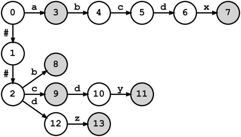
(a) The vocabulary and the corresponding trie.

$\boldsymbol{v}$	0	1	2
$\boldsymbol{F(v)}$	$\operatorname{[\,]}$	$\operatorname{[\,]}$	$\operatorname{[\,]}$
$\boldsymbol{f(v)}$	$\operatorname{\varnothing}$	$\operatorname{\varnothing}$	$\operatorname{\varnothing}$
$\boldsymbol{v}$	3	4	5		6		7
$\boldsymbol{F(v)}$	[a]	[a]	[a, ##b]		[a, ##b]		[abcdx]
$\boldsymbol{f(v)}$	2	8	9		10		2
$\boldsymbol{v}$	8	9	10	11		12		13
$\boldsymbol{F(v)}$	[##b]	[##c]	[##c]	[##cdy]		$\operatorname{[\,]}$		[##dz]
$\boldsymbol{f(v)}$	2	2	12	2		$\operatorname{\varnothing}$		2

(b) Complete table of $f(v)$ and $F(v)$.

Figure 1: Example vocabulary, the corresponding trie, and the table of auxiliary links and data. The suffix indicator is ##. Node 0 is the root node. Data nodes (in grey) indicate vocabulary tokens, i.e., the represented string is in $V$.

To motivate our linear algorithm, let’s first consider an alternative approach to MaxMatch using a simple vocabulary trie: when searching the longest token at a position, it starts from the shortest substring and iterates over the input text from left to right, following trie matching to find the longest prefixes that matches a vocabulary token.

Example 1.

Consider the vocabulary and the trie from Figure 1(a), with the input string abcdz. The expected output is $[\texttt{a},\texttt{\#\#b},\texttt{\#\#c},\texttt{\#\#dz}]$.

Starting from position 0, we follow the trie edges to match the input characters from a to d, arriving at node 6. No trie edge exits node 6 with character z as the label. The longest matching prefix seen so far is a, which is the first recognized token. ∎

The challenge of this approach is that, when the trie fails to match the next character, the longest vocabulary token match may be several characters back. As shown in Example 1, from position 0 we’ve matched the prefix abcd but found that the longest matching token is a. When looking for the next token, we reset the start position at character b and reprocess bcd.., resulting in repetitive and wasteful iterations. The time complexity is $O(nm)$.

The idea of LinMaxMatch is to use precomputed information to avoid reprocessing the characters.

Example 2.

For the same example as above, when the trie matching fails at character z, since abcd has been matched, given the vocabulary in use (Figure 1(a)), we should be able to know that the first two longest-matching tokens are $[\texttt{a},\texttt{\#\#b}]$. After collecting the tokens, we should reset our state as if we just matched ##cd and then continue to match the same character z. No need to reprocess bcd. ∎

Specifically, when trie matching arrives at node $v$ but cannot continue further, it must have matched the string represented by $v$ (i.e. $\chi_{v}$). We consider the tokens that MaxMatch would generate for the beginning of $\chi_{v}$ (called “failure pops” $F(v)$), which should be popped off the beginning of $\chi_{v}$ and put into the result. After that, we should transit to a state (following the “failure link” $f(v)$) that corresponds to the remaining suffix of $\chi_{v}$, from which the algorithm continues to match the next character. $F(v)$ and $f(v)$ are defined as below and can be precomputed based on the vocabulary.

Definition 1.

Failure links and pops. Given a node $v$ and the corresponding string $\chi_{v}$, consider the shortest non-empty list of longest-matching-prefix tokens $[p_{1},p_{2},...,p_{k}]$ (where $p_{i}\in V$, $p_{i}\neq\varepsilon$ or $\operatorname{\sharp}$, for $1\leq i\leq k$) that we can remove from $\chi_{v}$ (in order) until the remaining suffix can be represented by some node $v^{\prime}$ from the trie.

We define failure pops for node $v$ as $F(v)=[p_{1},p_{2},...,p_{k}]$ and failure link as $f(v)=v^{\prime}$.

If such a non-empty list $[p_{1},p_{2},...,p_{k}]$ does not exist, we define $f(v)=\operatorname{\varnothing}$. $F(v)$ is undefined and unused in this case. ∎

Put it another way, $F(v)$ and $f(v)$ are defined by finding the longest prefix of the string $\chi_{v}$ that matches a vocabulary token, popping it, and repeating this procedure until the suffix string is found on the trie. Figure 1(b) shows $F(v)$ and $f(v)$ computed for the example vocabulary and trie.

For readers with the background of finite-state transducers (FSTs) Mohri (1997), it’s helpful to see that $f(v)$ is related to the state transition function and $F(v)$ is related to the output function (more discussions in Section 3.6).

3.3 LinMaxMatch Tokenization

Assume that, based on the vocabulary, we have precomputed the trie, failure links, and failure pops (precomputation is discussed in Section 3.4). Given an input string, we follow the trie edges to process the input characters one by one. When trie matching cannot continue from node $v$, we make a failure transition in two steps: (1) retrieve failure pops $F(v)$ and append to the end of tokenization result, and (2) follow the failure link to node $f(v)$. After that, we continue from the new node $f(v)$.

Algorithm 1 shows the tokenization algorithm. For now, ignore lines 1-1; we explain it later.

Function LinMaxMatch($w$):

1    tokens, $u$, $i$ $\leftarrow$ MatchLoop$(w\texttt{\char 32\relax}{},0)$

2    if $i<|w|$ or $u\notin\{r,r_{\operatorname{\sharp}}\}$  then

3      tokens $\leftarrow[\operatorname{\texttt{<unk>}}]$

4   else if  $u=r_{\operatorname{\sharp}}\textbf{ and }|\text{tokens}|=0$  then

5       tokens $\leftarrow\textsc{OriginalWordPiece}(\operatorname{\sharp})$

6   return tokens

Function MatchLoop($s$, $i$):

7    $u,\text{tokens}$ $\;\leftarrow\;$ $r,\operatorname{[\,]}$

8    while $i<|s|$  do

9       while $\delta(u,s[i])=\operatorname{\varnothing}$  do

10          if $f(u)=\operatorname{\varnothing}$ then  return tokens, $u$, $i$

11          tokens $\leftarrow$ Extend(tokens, $F(u)$)

12          $u\leftarrow$ $f(u)$

13         

14      $u\leftarrow$ $\delta(u,s[i])$

15       $i\leftarrow i+1$

16   return tokens, $u$, $i$

Algorithm 1 LinMaxMatch Tokenization

The main function calls MatchLoop() with two inputs: $w$ appended by a whitespace ␣ and the start position 0 (line 1). Inside that function, let’s use the term step to denote an iteration of the loop on lines 1-1, which processes one input character $s[i]$. Each step starts from the current node $u$ and follows $f(u)$ zero, one, or multiple times (line 1), appending the tokens in $F(u)$ to the result along the way (line 1), until it finds a trie edge that matches the current character (line 1) or $f(u)=\operatorname{\varnothing}$ (line 1).

If the input string $w$ can be tokenized, the loop continues until $i\!=\!|s|\!-\!1$ pointing to the final appended whitespace. We know that $\delta(u,\texttt{\char 32\relax}{})=\operatorname{\varnothing}$ for any $u$ (since whitespace is not in any vocabulary token). MatchLoop() will keep following $f(u)$ while collecting $F(u)$ tokens along the way (line 1-1) until it arrives at $r_{\operatorname{\sharp}}$, where $f(r_{\operatorname{\sharp}})=\operatorname{\varnothing}$. MatchLoop() returns on line 1 with $u=r_{\operatorname{\sharp}}$, $i\!=\!|s|\!-\!1\!=\!|w|$, and tokens being the expected result (see Example 3). If $w=\varepsilon$, MatchLoop() returns immediately with $u=r$, $i\!=\!0\!=\!|w|$, and empty tokens. In either case, the tokens are returned by the main function (line 1).

On the other hand, if the word cannot be tokenized, when MatchLoop() returns on line 1, there are two cases: (1) Some normal input character cannot be consumed after attempting failure transitions (i.e., $i\!<\!|w|$). (2) $i\!=\!|w|$ but the final landing node $u\notin\{r,r_{\operatorname{\sharp}}\}$ representing a non-empty string $\chi_{u}$ yet $f(u)=\operatorname{\varnothing}$; according to Definition 1, $\chi_{u}$ cannot be tokenized. In either case, the result tokens are reset to $[\operatorname{\texttt{<unk>}}]$ (line 1). See Example 4.

Line 1 is only for safety reasons; it will not be visited since a whitespace is appended at the end.

Example 3.

Consider $s=w\texttt{\char 32\relax}{}=\texttt{abcdz{\char 32\relax}{}}$, using the vocabulary from Figure 1(a). The expected tokenization is $[\texttt{a},\texttt{\#\#b},\texttt{\#\#c},\texttt{\#\#dz}]$.

step	$i,s[i]$	node transition		result tokens
			0	$\operatorname{[\,]}$
1	0, a	$\delta(0,\texttt{a})$	$\rightarrow$ 3	$\operatorname{[\,]}$
2	1, b	$\delta(3,\texttt{b})$	$\rightarrow$ 4	$\operatorname{[\,]}$
3	2, c	$\delta(4,\texttt{c})$	$\rightarrow$ 5	$\operatorname{[\,]}$
4	3, d	$\delta(5,\texttt{d})$	$\rightarrow$ 6	$\operatorname{[\,]}$
5	4, z	$f(6)$	$\rightarrow$ 10	[a,##b]
		$f(10)$	$\rightarrow$ 12	[a,##b,##c]
		$\delta(12,\texttt{z})$	$\rightarrow$ 13	[a,##b,##c]
6	5, ␣	$f(13)$	$\rightarrow$ 2	[a,##b,##c, ##dz]
		$f(2)=\operatorname{\varnothing}$		[a,##b,##c, ##dz]

Table 2: Sequence of node transitions and result tokens.

Table 2 shows the sequence of node transitions and result tokens in MathLoop(). The first row is the original state. Steps 1-4 are self-explanatory.

Step 5 is more complex: when we reach step 5, the prefix abcd has already been processed. The current node is node 6, and the next character is z. As $\delta(6,\texttt{z})=\operatorname{\varnothing}$, we copy $F(6)$ to the result (which becomes [a, ##b]) and follow $f(6)$ to node 10. Next, as $\delta(10,\texttt{z})=\operatorname{\varnothing}$, we copy $F(10)$ to the result (which becomes [a, ##b, ##c]) and follow $f(10)$ to node 12. Now, as $\delta(12,\texttt{z})=13$, we follow the trie edge to node 13 and proceed to step 6.

Step 6 processes ␣. We first follow $f(13)$ to node 2, appending ##dz to the result tokens. Then, at node 2 (i.e., $u=2=r_{\operatorname{\sharp}}$), $\delta(u,\texttt{\char 32\relax}{})=\operatorname{\varnothing}$ and $f(u)=\operatorname{\varnothing}$. MatchLoop() returns on line 1.

Back to the main function (line 1), since $i\!=\!5\!=\!|w|$ (meaning that MatchLoop() stopped at the final whitespace) and $u=r_{\operatorname{\sharp}}$ (meaning that all matched characters abcd are covered by the result tokens), the word is successfully tokenized. It returns [a, ##b, ##c, ##dz] as expected. ∎

Example 4.

Consider two input words $s_{1}\!=\!w_{1}\texttt{\char 32\relax}{}\!=\!\texttt{abcz}\texttt{\char 32\relax}{}$, $s_{2}\!=\!w_{2}\texttt{\char 32\relax}{}\!=\!\texttt{abcd}\texttt{\char 32\relax}{}$. Using the same vocabulary, neither $w_{1}$ nor $w_{2}$ can be tokenized.

For $s_{1}$, MatchLoop() consumes abc but not z. Hence it stops within the word: $i=3<|w_{1}|$.

For $s_{2}$, MatchLoop() consumes all normal characters abcd but not the whitespace ␣. When it returns on line 1, $i=|w_{2}|$, $u$ is node 12 (since $f(12)\!=\!\operatorname{\varnothing}$), and the result tokens are $[\texttt{a},\texttt{\#\#b},\texttt{\#\#c}]$, which do not cover character d. Actually, the string ##d represented by node 12 cannot be tokenized.

Tokens are reset to $[\operatorname{\texttt{<unk>}}]$ in both cases. ∎

Corner cases

One behavior of the original WordPiece algorithm Google (2018) is that, if the input starts with the suffix indicator, the first result token may start with the suffix indicator. For example, in Figure 1, if the input is ##bc, the tokenization result is [##b, ##c]. In this paper, by having $r_{\operatorname{\sharp}}$ as a descendant of $r$, LinMaxMatch follows the same behavior and returns the same result.

Because $r_{\operatorname{\sharp}}$ is set as a descendant of $r$, if the input $w$ is $\operatorname{\sharp}$ itself (e.g., ##), normally Algorithm 1 would have returned an empty list of tokens, which is inconsistent with Google (2018). We handle this as a special case. Line 1 checks whether $w$ is $\operatorname{\sharp}$ by the following (instead of directly comparing the strings): if and only if $w=\operatorname{\sharp}$, the landing node $u$ is $r_{\operatorname{\sharp}}$ and the result tokens are empty after consuming all normal input characters (i.e., $i=|w|$). If so, the tokens are reset by the precomputed result of the original WordPiece algorithm on $\operatorname{\sharp}$ (line 1).

Algorithm 1 can be proved to be consistent with the original WordPiece algorithm Google (2018).

3.4 LinMaxMatch Precomputation

Given a vocabulary, it is straightforward to build the trie. This section explains how to precompute failure links $f(\cdot)$ and failure pops $F(\cdot)$.

We could compute $f(\cdot)$ and $F(\cdot)$ by directly using the procedure from Definition 1. Instead, we propose a faster algorithm (see Section 3.5 for complexity). Our algorithm computes $f(v)$ and $F(v)$ by leveraging $f(u)$ and $F(u)$ from the parent node $u$. Suppose $\delta(u,c)=v$. Intuitively, as the string $\chi_{u}$ of parent $u$ is a prefix of the string $\chi_{v}$ of node $v$, it is likely that $F(u)$ and $F(v)$ share some common longest-matching-prefixes in the beginning. It can be proved that when $\chi_{v}\notin V$, $F(v)$ consists of (1) the tokens from $F(u)$, followed by (2) the longest-matching-prefixes that the procedure from Definition 1 generates for the string $\chi_{f(u)}c$. Otherwise, when $\chi_{v}\in V$, it’s trivial that $F(v)=[\chi_{v}]$ based on Definition 1. Notice that $f(v)$ and $F(v)$ are computed using similar information for nodes that have strictly smaller depth than $v$. Breadth-First-Search (BFS) is suitable for the computation.

Algorithm 2 is the precomputation algorithm. On line 2, the algorithm builds a trie for $V$ and keeps track of $r$ and $r_{\operatorname{\sharp}}$. These nodes have depth 0 and are the starting points for our BFS traversal (line 2). We assume that initially $f(v)=\operatorname{\varnothing}$ and $F(v)=\operatorname{[\,]}$ for every node $v$. The core part is in lines 2-2, which computes $f(v)$ and $F(v)$ as discussed earlier.

The rest of the algorithm handles technical details. E.g., if $\operatorname{\sharp}$ is the empty string, the nodes $r$ and $r_{\operatorname{\sharp}}$ are identical; accordingly, line 2 avoids duplicate nodes. Otherwise, $r_{\operatorname{\sharp}}$ is a descendant of $r$, and we need line 2 to avoid revisiting it in the BFS traversal.

It can be proved that Algorithm 2 correctly precomputes $f(v),F(v)$ for each trie node $v$.

Function Precompute($V$):

1    $r,r_{\operatorname{\sharp}}\leftarrow\textsc{Buildtrie}(V)$

2    queue $\leftarrow$ ($r_{\operatorname{\sharp}}\neq r$) ? [$r$, $r_{\operatorname{\sharp}}$] : [$r$]

3    while not Empty(queue) do

4       $u\leftarrow$ Dequeue(queue)

5       for $c,v$ in OutgoingEdges($u$) do

6          if $v=r_{\operatorname{\sharp}}$ then  continue

7          if $\chi_{v}\in V$  then

8             $f(v),F(v)\leftarrow r_{\operatorname{\sharp}},[\chi_{v}]$

9         else

10             $z,Z\leftarrow$ $f(u)$, $\operatorname{[\,]}$

11             while $z\neq\operatorname{\varnothing}$ and $\delta(z,c)=\operatorname{\varnothing}$ do

12                $Z\leftarrow$ Extend(Z, $F(z)$)

13                $z\leftarrow f(z)$

14               

15            if $z\neq\operatorname{\varnothing}$ then

16                $f(v),F(v)\leftarrow\delta(z,c),F(u)+Z$

17               

18            

19         Enqueue(queue, $v$)

20      

21   return $r$

22   

Algorithm 2 Precomputation

3.5 Complexity Analysis

The complexity of tokenization (Algorithm 1) can be proved to be $O(n)$ in a similar way as Aho-Corasick Aho and Corasick (1975). In brief, each step (an iteration of the loop from lines 1-1) makes zero or more failure transitions followed by exactly one normal (non-failure) transition. In each step, suppose we start at node $u$ with depth $d$. We never follow more than $d$ failure transitions in that step: each failure transition takes us to a node with a strictly smaller depth. Any normal transition along trie edges increments the depth $d$ of node $u$ by 1 (line 1). Therefore, the total number of failure transitions is no more than the total number of normal transitions, which is $O(n)$. Each transition is $O(1)$ plus the work to extend the list of tokens on line 1. As there are at most $n$ resulting tokens in total, the total tokenization time is $O(n)$.

Since at least $n$ operations are required to read the entire input, our $O(n)$ algorithm is asymptotically optimal. To the best of our knowledge, this is the first time that the optimal complexity for MaxMatch is proved to be strictly $O(n)$, without a vocabulary-specific multiplicative factor.

For precomputation (Algorithm 2), the BFS traversal itself is $O(M)$, where $M$ is the sum of the lengths of vocabulary tokens. A similar depth-based analysis (as in the case of the tokenization algorithm) shows that that the total number of times we traverse a failure link on line 2 is $O(M)$.

The non-trivial parts are the construction of $F(\cdot)$ on lines 2 and 2. The total size of $F(\cdot)$ is $O(Mm)$: there are $O(M)$ lists, and the size of each list is $O(m)$. A straightforward implementation needs $O(Mm)$ time and space to construct and store $F(\cdot)$. This is good enough in practice, as the precomputation is performed offline before any tokenization process. We plan to discuss optimized implementations in a follow-up publication.

3.6 Connection with Other Methods / Tasks

LinMaxMatch can be turned into a finite-state transducer (FST) Mohri (1997) by eliminating the failure transitions in Algorithm 1. An FST extends a finite-state automaton (FSA) with an output tape. To turn LinMaxMatch into an FST, for node $u$ and character $c$, we define the state transition function $\delta^{\prime}(u,c)$ and the output function $\sigma^{\prime}(u,c)$ as follows:

• $\delta^{\prime}(u,c)$ precomputes the final state in lines 1-1 of Algorithm 1, where it starts from $u$ and follows failure transitions as needed, until it consumes $c$ or meets a null failure link;

• $\sigma^{\prime}(u,c)$ consists of the failure pops collected along the way.

Specially, if the original trie link $\delta(u,c)$ exists, according to the above definition, it’s obvious that $\delta^{\prime}(u,c)=\delta(u,c)$ and $\sigma^{\prime}(u,c)=[]$. Then lines 1-1 in Algorithm 1 can be replaced with two statements: $\text{tokens}\leftarrow\textsc{Extend}(\text{tokens},\sigma^{\prime}(u,s[i]))$ and $u\leftarrow\delta^{\prime}(u,s[i])$; the loop (started on line 1) breaks when $u$ becomes $\operatorname{\varnothing}$. Hence, LinMaxMatch makes exactly one state transition on each input character. Obviously, the time complexity is linear, despite more space needed to store precomputed results.

LinMaxMatch extends the Aho-Corasick Algorithm (Aho and Corasick, 1975). It can be applied to more string search or transducer problems. Let us name a few here. LinMaxMatch can be adapted to solve the multi-keyword search problem which Aho-Corasick is designed for. It can be also adapted to address other MaxMatch variants, such as Backward MaxMatch Webster and Kit (1992), recognizing unseen characters as single-character tokens Palmer (2000), or combing with transformation rules Sassano (2014). Other potential applications include word segmentation in Asian languages Sassano (2014), phonological or morphological analysis Kaplan and Kay (1994); Jurafsky and Martin (2009).

4 Linear-Time End-to-End Tokenization

The existing BERT tokenization implementations Google (2018) pre-tokenize the input text (splitting it into words by punctuation and whitespace characters) and then call WordPiece tokenization on each resulting word. For example, the text john johanson’s may be split into [john, johan, ##son, ’, s].

We propose an end-to-end WordPiece tokenizer that combines pre-tokenization and WordPiece into a single, linear-time pass. It uses the LinMaxMatch trie matching and failure transition loop as much as possible and only checks for punctuation and whitespace characters among the relatively few input characters that are not handled by the loop. It is more efficient as it traverses the input only once, performs fewer punctuation / whitespace checks, and skips the creation of intermediate words.

Precomputation

We use the same process as in Section 3.4, with several differences:

After the trie is constructed, we remove all trie links labeled with a punctuation character. Then, for every possible punctuation character $c$, we add a trie data node $v$ with no descendants, and a trie link from the root $r$ to $v$ with label $c$. If $c$ is part of the vocabulary, we set $\chi_{v}=c$, otherwise $\chi_{v}=\operatorname{\texttt{<unk>}}$.

The resulting trie matches all punctuation characters, as either themselves or as $\operatorname{\texttt{<unk>}}$, depending on the vocabulary. Punctuation characters are not part of longer tokens, and there is no suffix token for a punctuation character. This reflects the fact that each punctuation character is a word by itself.

We then run the rest of Algorithm 2 to compute the failure pops and failure links.

Finally, for punctuation nodes, we set their failure links to a special node $r_{p}$; their failure pops are not changed. The special node $r_{p}$ has no parent and no descendants, and $\chi_{r_{p}}=\varepsilon,f(r_{p})=\operatorname{\varnothing}$. Node $r_{p}$ indicates that a punctuation character was matched.

Tokenization

Algorithm 3 tokenizes general text into wordpieces. It starts by appending a whitespace ␣ at the end of the input (line 3). In each iteration, it recognizes wordpieces for the current word by employing (almost) the same routine as in single-word tokenization (lines 3-3 in Algorithm 3 versus lines 1-1 in Algorithm 1).

When returning from MatchLoop(), Algorithm 3 must have met a character that cannot be consumed after attempting failure transitions, such as a whitespace, a punctuation, or some unseen character. Lines 3-3 examine whether the current word can be tokenized (by checking if the current position is at a word boundary and where the node $u$ lands at) and reset the tokens as appropriate (see related discussions in Section 3.3).

Lines 3-3 further handle the corner case that the word happens to be the suffix indicator itself (in the same way as Algorithm 1, see Section 3.3). Note that normally the suffix indicator contains only punctuation characters (e.g., ## in BERT); in that case lines 3-3 can be saved, because the suffix indicator itself is not be tokenized as a single word.

The tokens of the current word are then appened to the result (line 3). Finally, the algorithm moves the cursor past the boundary of the current word (lines 3-3) and skips any following whitespaces (lines 3-3) to process the next word.

It can be shown that Algorithm 3 is consistent with Google (2018) for general text tokenization, and the time complexity is $O(n)$.

Function E2EWordPiece(text) :

1   

2   $\text{result},\;s,\;i\leftarrow\operatorname{[\,]},\;\text{text}\texttt{\char 32\relax}{},\;0$

3    while ${i}<|s|$  do

4       $\text{tokens},u,i\leftarrow\textsc{MatchLoop}(s,i)$

5       if not IsWdBndry($s,\!i$) or $\!u\!\notin\!\{r,\!r_{\!\operatorname{\sharp}},\!r_{p}\!\}\!\!$  then

6          tokens $\leftarrow[\operatorname{\texttt{<unk>}}]$

7      else if  $u=r_{\operatorname{\sharp}}\textbf{ and }|\text{tokens}|=0$  then

8          tokens $\leftarrow\textsc{OriginalWordPiece}(\operatorname{\sharp})$

9      result $\leftarrow$ Extend(result, tokens)

10       while $i\!<\!|s|$ and not IsWdBndry($s,i$) do

11          $i\leftarrow i+1$

12      while $i<|s|$ and IsSpace$(s[i])$ do

13          $i\leftarrow i+1$

14      

15   return result

Function IsWdBndry($s$, $i$):

16    return $i\!\geq\!|s|$ or ($i\!>\!0$ and IsPunc$(s[i\!-\!1])$) or IsSpace$(s[i])$ or IsPunc$(s[i])$

Algorithm 3 End-to-End Tokenization

5 Experiments

Experimental Setup

We benchmark our method against two widely-adopted WordPiece tokenization implementations:

• HuggingFace Tokenizers HuggingFace (2020), from the HuggingFace Transformer library, one of the most popular open-source NLP tools.

• TensorFlow Text Google (2020), the official library of text utilities for TensorFlow.

In both cases, we use pre-tokenization and WordPiece tokenization, and skip other steps provided by those libraries (text cleanup, normalization, etc) for fair comparison. Both libraries use the original WordPiece tokenization algorithm Google (2018). They both generate not only the numeric ids of the tokens, but also the token strings and start/end offsets of the input word. We modify both libraries to generate only the token ids, for two reasons: (1) most downstream models (e.g., BERT) consume only the token ids, and (2) we want to focus on the core tokenization work, not on, e.g., string copying.

We implement LinMaxMatch and E2E WordPiece and made them return the numeric ids of the tokens, leveraging a double array-based trie library Yata et al. (2007).

We compare our algorithms with HuggingFace and TensorFlow Text on a large corpus (several million words) and found that the tokenization results are identical for both single-word and end-to-end tokenization. In the rest of this section, we focus on the tokenization speed.

All experiments are conducted on a Linux desktop with a six-core Intel Xeon @ 3.60GHz CPU and 64GB memory. We iterate each benchmark (after warming up) until it ran for a long-enough period of time, repeat each experiment 10 times, and report the average results. Our method is implemented and benchmarked in C++; so is TensorFlow Text. HuggingFace uses (and is benchmarked in) Rust.

We use the WordPiece vocabulary released with the BERT-Base, Multilingual Cased model, a model that supports 104 languages Google (2018).

To generate the test data, we sample 1,000 sentences from the multilingual Wikipedia dataset, covering 82 languages including English, Chinese, French, Russian, etc. On average, each word has 4 characters, and each sentence has 82 characters or 17 words. We found this dataset large enough: a much larger dataset (consisting of hundreds of thousands of sentences) generated similar results.

We run BERT’s BasicTokenizer Google (2018) to clean up and normalize each sentence, including Unicode clean-up and normalization. Following the guidance for the BERT-Base Multilingual Cased model Google (2018), we do not instruct BasicTokenizer to do lower casing or accent stripping. In addition, preprocessing adds spaces around every CJK character, and thus Chinese is effectively character-tokenized. For simplicity, we keep Chinese in the test set, but keep in mind that each Chinese word is just one Chinese character, and any WordPiece implementation is efficient on such short words. Using a dataset with long words would emphasize the speed advantage of our algorithm even more than indicated below.

For single-word tokenization, we further used BasicTokenizer to pre-tokenize each sentence on punctuation and whitespace characters. This results in 17,223 words, 8,508 of them unique.

Results

Table 3 shows the mean and the 95 percentile running time when tokenizing a single word or general text (end-to-end) for each system. For single-word tokenization, ours is 3x faster on average; the speedup is greater for long-tail inputs. Regarding general text end-to-end tokenization, ours is 8.2x faster than HuggingFace and 5.1x faster than TensorFlow Text on average. Figure 2 shows how the running time grows with respect to the input length for single-word tokenization.

System	Single Word		End-to-End
	mean	95pctl	mean	95pctl
HuggingFace	274	778	13,397	40,255
TensorFlow Text	246	622	8,247	23,507
Ours	82	139	1,629	4,400

Table 3: The running time of each system in ns.

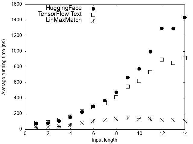
Figure 2: Average running time of each system with respect to the input length for single-word tokenization.

6 Conclusion

We proposed LinMaxMatch for single-word WordPiece tokenization, which is asymptotically-optimal linear-time with respect to the input length, without a vocabulary-specific multiplicative factor. We also proposed E2E WordPiece that combines pre-tokenization and WordPiece tokenziation into a single, linear-time pass for even higher efficiency. Experimental results show that our approach is 8.2x faster than HuggingFace and 5.1x faster than TensorFlow Text on average for general text tokenization. For future work, we will adapt the proposed methods to more text processing techniques.

7 Acknowledgements

We thank Xiaoxue Zang, Gabriel Schubiner, Max Gubin, Jacob Devlin, Kristina Toutanova, and Ed Chi for discussing and reviewing the work, Mike Schuster for clarifying their referred paper, and the anonymous reviewers for their helpful feedback.

Appendix A Mathematical Formulations and Proofs of LinMaxMatch

In this section, we present the mathematical formulations of the proposed LinMaxMatch algorithm and prove the correctness.

We introduce more notations here.

Definition 2.

The length of string $w$ is $|w|$ (i.e., the number of characters in $w$) if $w$ does not start with $\operatorname{\sharp}$; otherwise, its length is $|w|-|{\operatorname{\sharp}}|$. ∎

For example, the length of abc is 3, the length of ##d is 1 (where ## is the suffix indicator), and the length of $\varepsilon$ or $\operatorname{\sharp}$ is 0.

Definition 3.

Given vocabulary $V$, let ${p_{w}}$ be the longest non-empty prefix of $w$ that is in $V$. That is,

$$p_{w}\eqdef\arg\max_{w^{\prime}}\big{\{}|w^{\prime}|\mid \;w^{\prime}\text{ is a prefix of }w,$$

$$\;w^{\prime}\in V,w^{\prime}\notin\{\varepsilon,\operatorname{\sharp}{}\}\big{\}}$$

Specially, $p_{w}\eqdef\varepsilon$ if no such prefixes exist. In addition, if $w$ starts with $\operatorname{\sharp}$, the prefix $p_{w}$ should also start with $\operatorname{\sharp}$ (unless $p_{w}$ is empty). When $w=\operatorname{\sharp}$, $p_{\operatorname{\sharp}}\eqdef\varepsilon$ for clarity. ∎

Definition 4.

Let $q_{w}$ be the suffix of $w$ after replacing the prefix $p_{w}$ with $\operatorname{\sharp}$. That is, if $w=p_{w}w^{\prime\prime}$, $q_{w}\eqdef\operatorname{\sharp}w^{\prime\prime}$. ∎

For example, if $V=\{\texttt{a},\texttt{ab},\texttt{\#\#c}\}$, let the suffix indicator $\operatorname{\sharp}$ be ##, then $p_{\texttt{abcd}}=\texttt{ab}$, $q_{\texttt{abcd}}=\texttt{\#\#cd}$, $p_{\texttt{\#\#cd}}=\texttt{\#\#c}$, and $q_{\texttt{\#\#cd}}=\texttt{\#\#d}$. We see that if $w\in V$, $p_{w}=w$ and $q_{w}=\operatorname{\sharp}$.

Lemma 1.

For an nonempty string $wc$, where $c$ is the last character and $w$ is the prefix ($w$ could be $\varepsilon$ or $\operatorname{\sharp}$), if $wc\notin V$, we have $p_{wc}=p_{w}$ and $q_{wc}=q_{w}c$.

Sketch of Proof.

First, we prove that $p_{wc}$ does not include the last character $c$ by contradiction. Let’s suppose that $p_{wc}$ includes the last character $c$. Then $p_{wc}=wc$ (since $p_{wc}$ is a prefix of $wc$). Because $p_{wc}\in V$ (Definition 3), $wc\in V$, which contradicts that $wc\notin V$.

Now, because $p_{wc}$ does not include the last character $c$, it is obvious that $p_{wc}=p_{w}$.

Next, let $w=p_{w}w^{\prime\prime}$, then $q_{w}=\operatorname{\sharp}{}w^{\prime\prime}$ (Definition 4). Since $p_{wc}=p_{w}$, we have $wc=p_{w}w^{\prime\prime}c=p_{wc}w^{\prime\prime}c$. Therefore, $q_{w}=\operatorname{\sharp}{}w^{\prime\prime}c=q_{w}c$. ∎

Let $\gamma_{w}$ denote the trie node that represents the string $w$ (so $\chi_{\gamma_{w}}=w$), or $\operatorname{\varnothing}$ if no such nodes exist. When $\gamma_{w}\neq\operatorname{\varnothing}$, we say the string $w$ is on the trie. For the example in Figure 1, $\gamma_{\texttt{abcd}}$ is the node 6 while $\gamma_{\texttt{abcdz}}=\operatorname{\varnothing}$.

Table 4 summarizes the additional notations.

Symbol	Meaning
$p_{w}$	The longest prefix of $w$ being in $V$
$q_{w}$	The suffix of $w$ after removing prefix
	$p_{w}$, plus a preceding $\operatorname{\sharp}$
$M(w)$	MaxMatch result for $w$ given $V$
$\gamma_{w}$	The node that represents string $w$
$g(w)$	MinPop Matching $w$ onto some node
$G(w)$	Tokens popped when computing $g(w)$
$h(u,c)$	$g(\chi_{u}c)$ (or $\operatorname{\varnothing}$ if $u=\operatorname{\varnothing})$
$H(u,c)$	$G(\chi_{u}c)$ (or $\operatorname{[\,]}$ if $u=\operatorname{\varnothing}$)

Table 4: Additional Notations (continued from Table 1)

A.1 MaxMatch in WordPiece

MaxMatch in WordPiece tokenization Google (2018) can be formalized as follows:

Definition 5.

MaxMatch

Given vocabulary $V$, for string $w$, MaxMatch $M(w)$ is recursively defined as:

$$M(w)\!\eqdef\!\begin{cases}\operatorname{[\,]}&\text{if }w=\varepsilon\text{ or }\operatorname{\sharp},\\ [\operatorname{\texttt{<unk>}}]&\text{elif }p_{w}=\varepsilon,\\ [\operatorname{\texttt{<unk>}}]&\text{elif }M(q_{w})=[\operatorname{\texttt{<unk>}}],\\ [p_{w}]\!+\!M(q_{w})\!\!\!&\text{otherwise}.\end{cases}$$ (1)

∎

Note that if the input is exactly the suffix indicator $\operatorname{\sharp}$ itself, by Definition 5, $M(\operatorname{\sharp})\eqdef\operatorname{[\,]}$, which may be different from the original MaxMatch algorithm Google (2018) (see Sec. 3.3). Throughout this section, we focus on Definition 5, but be aware that if the original input is exactly the suffix indicator, we resort to the original MaxMatch algorithm.

A.2 MinPop Matching

We introduce a few concepts and discuss their properties and relationships, as shown in Figure 3, which eventually lead to the mathematical formulation of the algorithm and the proofs.

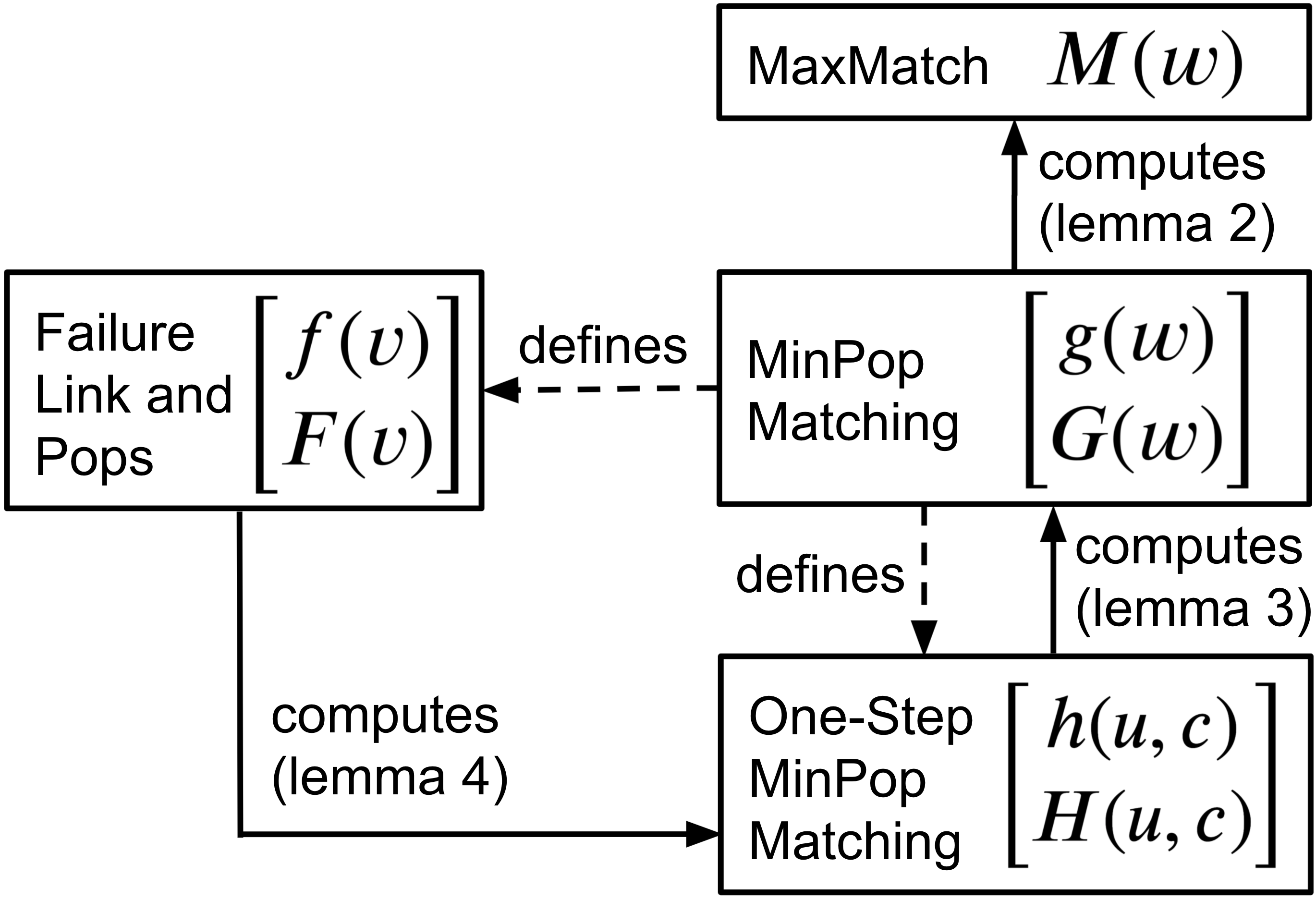
Figure 3: Definitions and the relationships.

The first concept is MinPop Matching, which means "minimally popping longest-matching prefixes off the beginning of a string until matching a trie node". The formal definition is as follows:

Definition 6.

MinPop Matching

For a string $w$, define:

• $g(w)$: returns a node that represents $w$ if possible, or a node pointing to the suffix of $w$ after popping the least number of consecutive prefixes following the left-to-right longest-match-first process if possible, otherwise $\operatorname{\varnothing}$.

• $G(w)$: returns the list of consecutive longest-matching prefix tokens that are popped when computing $g(w)$.

$$\begin{bmatrix}g(w)\\ G(w)\end{bmatrix}\!\eqdef\!\begin{cases}\!\begin{bmatrix}\gamma_{w}\\ [\;]\end{bmatrix}&\text{if }\gamma_{w}\neq\operatorname{\varnothing},\\[11.38109pt] \!\begin{bmatrix}\operatorname{\varnothing}\\ [\;]\end{bmatrix}&\text{elif }p_{w}=\varepsilon,\\[11.38109pt] \!\begin{bmatrix}g(q_{w})\\ [p_{w}]\!+\!G(q_{w})\end{bmatrix}&\text{otherwise.}\\ \end{cases}$$ (2)

∎

Example 5.

Table  5 shows $g(w)$ and $G(w)$ of example strings using the vocabulary in Figure 1. ∎

$\boldsymbol{w}$	abcd	##bcd	##cdz	##bcdz	z
$\boldsymbol{g(w)}$	6	10	13	13	$\operatorname{\varnothing}$
$\boldsymbol{G(w)}$	$\operatorname{[\,]}$	[##b]	[##c]	[##b, ##c]	[]

Table 5: Examples of $g(w)$ and $G(w)$ for Figure 1

Note that if $w$ is on the trie, no popping is needed when computing $g(w)$ and $G(w)$. See Example 5.

MinPop Matching provides an alternative way to compute MaxMatch as shown in Lemma 2.

Lemma 2.

For ease of presentation, we augment the trie by adding two nodes representing ␣ and $\operatorname{\sharp}\texttt{\char 32\relax}{}$, respectively, where ␣ is the whitespace character that is not in the alphabet of the vocabulary. Note that although ␣ and $\operatorname{\sharp}\texttt{\char 32\relax}{}$ are on the trie, the two strings are not added to the vocabulary. Figure 4 shows the augmented trie built from the example vocabulary in Figure 1. Then MaxMatch $M(w)$ can be equivalently computed as:

$$M(w)=\begin{cases}[\operatorname{\texttt{<unk>}}]&\text{if }g(w\texttt{\char 32\relax}{})=\operatorname{\varnothing},\\ G(w\texttt{\char 32\relax}{})&\text{otherwise}.\end{cases}$$ (3)

Sketch of Proof.

If $w$ is either $\varepsilon$ or $\operatorname{\sharp}$, it’s straightforward that $g(w\texttt{\char 32\relax}{})$ is $\gamma_{\texttt{\char 32\relax}{}}$ or $\gamma_{\operatorname{\sharp}\texttt{\char 32\relax}}$, which is not $\operatorname{\varnothing}$ on the augmented trie, and $G(w\texttt{\char 32\relax}{})=[]=M(w)$.

Let $w\notin\{\varepsilon,\operatorname{\sharp}\}$. Since ␣ is not in the vocabulary alphabet, $w\texttt{\char 32\relax}{}$ is not on the trie (i.e., $\gamma_{w\texttt{\char 32\relax}{}}=\operatorname{\varnothing}$).

If $w$ can be successfully tokenized, according to Equation 2, it will keep popping the longest-matching prefixes until the remaining suffix becomes $\operatorname{\sharp}\texttt{\char 32\relax}{}$, which is on the augmented trie. Hence, $g(w\texttt{\char 32\relax}{})$ becomes $\gamma_{\sharp\texttt{\char 32\relax}{}}$ ($\neq\operatorname{\varnothing}$), and $G(w\texttt{\char 32\relax}{})$ equals to $M(w)$.

Otherwise, by Equation 2, at some point $p_{w}$ will be $\varepsilon$; thus, $g(w\texttt{\char 32\relax}{})$ will eventually be $\operatorname{\varnothing}$. Equation 3 returns $[\texttt{<unk>}]$, which equals to $M(w)$. ∎

$\boldsymbol{V}$: $\left\{\texttt{a},\,\texttt{abcdx},\,\texttt{\#\#b},\,\texttt{\#\#c},\,\texttt{\#\#cdy},\,\texttt{\#\#dz}\right\}$

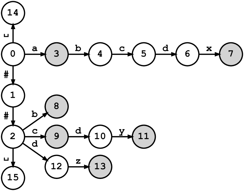
(a) The vocabulary and the augmented trie.

$\boldsymbol{v}$	0	1	2	14		15
$\boldsymbol{F(v)}$	$\operatorname{[\,]}$	$\operatorname{[\,]}$	$\operatorname{[\,]}$	$\operatorname{[\,]}$		$\operatorname{[\,]}$
$\boldsymbol{f(v)}$	$\operatorname{\varnothing}$	$\operatorname{\varnothing}$	$\operatorname{\varnothing}$	$\operatorname{\varnothing}$		$\operatorname{\varnothing}$
$\boldsymbol{v}$	3	4	5		6		7
$\boldsymbol{F(v)}$	[a]	[a]	[a, ##b]		[a, ##b]		[abcdx]
$\boldsymbol{f(v)}$	2	8	9		10		2
$\boldsymbol{v}$	8	9	10	11		12		13
$\boldsymbol{F(v)}$	[##b]	[##c]	[##c]	[##cdy]		$\operatorname{[\,]}$		[##dz]
$\boldsymbol{f(v)}$	2	2	12	2		$\operatorname{\varnothing}$		2

(b) Complete table of $f(v)$ and $F(v)$.

Figure 4: Augmented trie of the same example vocabulary and the table of failure links and failure pops. Compared to Figure 1, nodes 14 and 15 are added representing ␣ and ##␣. By Definition 1 we see that for the added nodes (14 and 15), the failure links are $\operatorname{\varnothing}$ and failure pops are $\operatorname{[\,]}$. The remaining entries of $F(\cdot)$, $f(\cdot)$ remain the same.

Example 6.

In Figure 4, $M(\texttt{abcdx})=G(\texttt{abcdx}\texttt{\char 32\relax}{})=[\texttt{abcdx}]$ since $g(\texttt{abcdx}\texttt{\char 32\relax}{})$ is node 15 ($\neq\operatorname{\varnothing}$). $M(\texttt{z})=[\operatorname{\texttt{<unk>}}]$ since $g(\texttt{z}\texttt{\char 32\relax}{})=\operatorname{\varnothing}$. ∎

A.3 One-Step MinPop Matching

Given that MaxMatch $M(w)$ can by computed via MinPop Matching (Lemma 2), we now discuss how to efficiently compute $g(w)$ and $G(w)$ via the concept of One-Step MinPop Matching.

Definition 7.

One-Step MinPop Matching

$h(u,c)$ and $H(u,c)$ capture this process: from node $u$, match one character $c$ by minimally popping longest-matching prefixes. Mathematically:

$$\begin{bmatrix}h(u,c)\\ H(u,c)\end{bmatrix}\!\eqdef\!\begin{cases}\begin{bmatrix}\operatorname{\varnothing}\\ \operatorname{[\,]}\end{bmatrix}&\text{if }u=\operatorname{\varnothing},\\[11.38109pt] \begin{bmatrix}g(\chi_{u}c)\\ G(\chi_{u}c)\end{bmatrix}&\text{otherwise}\end{cases}$$ (4)

∎

Example 7.

Table 6 shows some example values of $h(u,c)$ and $H(u,c)$ for Figure 4. ∎

$\boldsymbol{u}$	8	9	10	13	6	0
$\boldsymbol{c}$	c	d	z	␣	z	z
$\boldsymbol{h(u,c)}$	9	10	13	14	13	$\operatorname{\varnothing}$
$\boldsymbol{H(u,c)}$	[##b]	$\operatorname{[\,]}$	[##c]	[##dz]	[a, ##b, ##c]	[]

Table 6: Examples of $h(u,c)$ and $H(u,c)$ for Figure 4

Lemma 3 shows how to compute $g(w)$ and $G(w)$ efficiently using $h(u,c)$ and $H(u,c)$.

Lemma 3.

MinPop Matching $g(\cdot),G(\cdot)$ can be computed recursively as follows:

If the string is either $\varepsilon$ or $\operatorname{\sharp}$, $g(\varepsilon)=r$, $G(\varepsilon)=\operatorname{[\,]}$; $g(\operatorname{\sharp})=r_{\operatorname{\sharp}}$, $G(\operatorname{\sharp})=\operatorname{[\,]}$ (Definition 6).

Otherwise, the string contains at least one character. Let’s denote the string as $wc$, where $w$ is its prefix and $c$ is the last character. ($w$ could be $\varepsilon$ or $\operatorname{\sharp}$). Let $u=g(w)$, we have:

$$\begin{bmatrix}g(wc)\\ G(wc)\end{bmatrix}\!=\!\begin{bmatrix}h(u,c)\\ G(w)+H(u,c)\end{bmatrix}\\$$ (5)

Sketch of Proof.

We prove by induction on the length of the prefix string $w$. Note that the length of a string does not count the leading suffix indicator (Definition 2).

The basis is when the length of $w$ is 0, i.e., $w$ is either $\varepsilon$ or $\operatorname{\sharp}$. It’s trivial to verify that Equation 5 holds for the basis case.

For the inductive steps, let the length of $w$ be $k$ ($\geq 1$). Assume that Equation 5 holds for any string $w^{\prime}$ and character $c$ where the length of $w^{\prime}$ is smaller than $k$. There are three cases to discuss.

Case 1. $\gamma_{w}\neq\operatorname{\varnothing}$. In this case, $u=g(w)=\gamma_{w}\neq\operatorname{\varnothing}$, and $\chi_{u}=w$, $G(w)=\operatorname{[\,]}$. By Definition 7,

$$\begin{bmatrix}g(wc)\\ G(wc)\end{bmatrix}\!\!=\!\!\begin{bmatrix}g(\chi_{u}c)\\ G(\chi_{u}c)\end{bmatrix}\!\!=\!\!\begin{bmatrix}h(u,c)\\ H(u,c)\end{bmatrix}\!\!=\!\!\begin{bmatrix}h(u,c)\\ G(w)\!+\!H(u,c)\end{bmatrix}\!\!.$$

In the remaining two cases, $\gamma_{w}=\operatorname{\varnothing}$, hence $\gamma_{wc}=\operatorname{\varnothing}$, which means $wc\notin V$. Hence, $p_{wc}=p_{w}$ and $q_{wc}=q_{w}c$ (Lemma 1). When computing $g(wc)$ and $G(wc)$, since $\gamma_{wc}=\operatorname{\varnothing}$, by Equation 2, there are two remaining cases:

Case 2. $\gamma_{w}=\operatorname{\varnothing}$ and $p_{wc}=\varepsilon$. We have $p_{w}=p_{wc}=\varepsilon$, so by Equation 2 $g(w)=g(wc)=\operatorname{\varnothing}$ and $G(w)=G(wc)=\operatorname{[\,]}$. Since $u=g(w)=\operatorname{\varnothing}$, by Equation 4 $h(u,c)=\operatorname{\varnothing}$ and $H(u,c)=\operatorname{[\,]}$. Hence,

$$\begin{bmatrix}g(wc)\\ G(wc)\end{bmatrix}=\begin{bmatrix}\operatorname{\varnothing}\\ \operatorname{[\,]}\end{bmatrix}=\begin{bmatrix}h(u,c)\\ G(w)+H(u,c)\end{bmatrix}$$

Case 3. $\gamma_{w}=\operatorname{\varnothing}$ and $p_{wc}\neq\varepsilon$. Since $p_{wc}=p_{w}$, we have $q_{wc}=q_{w}c$, and $g(q_{w})=g(w)=u$. Since $q_{w}$ is a shorter string whose length is smaller than $k$, by the induction assumption, we have

$$\begin{bmatrix}g(q_{wc})\\ G(q_{wc})\end{bmatrix} =\begin{bmatrix}g(q_{w}c)\\ G(q_{w}c)\end{bmatrix}=\begin{bmatrix}h(u,c)\\ G(q_{w})+H(u,c)\end{bmatrix}$$

Hence,

$$\begin{bmatrix}g(wc)\\ G(wc)\end{bmatrix} =\begin{bmatrix}g(q_{wc})\\ [p_{wc}]+G(q_{wc})\end{bmatrix}$$ (Eq. 2)

$$=\begin{bmatrix}h(u,c)\\ [p_{w}]+G(q_{w})+H(u,c)\end{bmatrix}$$

$$=\begin{bmatrix}h(u,c)\\ G(w)+H(u,c)\end{bmatrix}$$ (Eq. 2)

Therefore, Equation 5 is proved. ∎

Example 8.

Take Figure 4 as an example, let $w=\texttt{\#\#bcd}$ and $c=\texttt{z}$. We know $u=g(w)$ is node 10 and $G(w)=[\texttt{\#\#b}]$ (Table 5). Given $u=10$ and $c=\texttt{z}$, we also know that $h(u,c)=h(10,\texttt{z})=13$ and $H(u,c)=H(10,\texttt{z})=[\texttt{\#\#c}]$ (Table 6). For $wc=\texttt{\#\#bcdz}$, we can see that $g(wc)=h(u,c)=13$, and $G(wc)=G(w)+H(u,c)=[\texttt{\#\#b}]+[\texttt{\#\#c}]=[\texttt{\#\#b},\texttt{\#\#c}]$. ∎

If we precompute and store $h(u,c),H(u,c)$ for every pair of node $u$ and character $c$, then for an arbitrary string $w$, we can efficiently compute $g(w\texttt{\char 32\relax}),G(w\texttt{\char 32\relax})$ (Lemma 3) and MaxMatch $M(w)$ (Lemma 2). This results in an algorithm that can be formualized as a finite-state transducer (FST) (more discussions in Section A.7). However, it needs more space to store the $h(u,c)$ and $H(u,c)$ tables. For example, the size of the $h(u,c)$ table is $O(|T|\cdot|\Sigma|)$, where $|T|$ is the size of the trie and $|\Sigma|$ is the size of the alphabet.

In the following sections, we show that, while maintaining the overall linear time complexity (Section 3.5), failure links $f(v)$ and failure pops $F(v)$ can be used to efficiently compute $h(u,c)$ and $H(u,c)$, but with much less space. For example, the size of $f(v)$ table is $O(|T|)$, which is much less than the $O(|T|\cdot|\Sigma|)$ space needed for the $h(u,c)$ table. This eventually results in Algorithm 1, which is a more practical approach.

A.4 Failure links and Failure Pops

The mathematical definition of $f(v)$ and $F(v)$ is:

Definition 8.

Failure links and pops (continued from Definition 1). Mathematically, let $w=\chi_{v}$, $f(v)$ and $F(v)$ are defined as follows:

$$\begin{bmatrix}f(v)\\ F(v)\end{bmatrix}\!\eqdef\!\begin{cases}\!\begin{bmatrix}\operatorname{\varnothing}\\ [\;]\end{bmatrix}&\text{if }p_{w}=\varepsilon,\\[11.38109pt] \!\begin{bmatrix}g\big{(}q_{w}\big{)}\\ \big{[}p_{w}\big{]}\!+\!G\big{(}q_{w}\big{)}\end{bmatrix}\!\!\!\!\!&\text{otherwise.}\\ \end{cases}$$ (6)

∎

Lemma 4 shows how to compute $h(u,c)$ and $H(u,c)$ recursively based on $f(\cdot)$ and $F(\cdot)$.

Lemma 4.

One-Step MinPop Matching $h(u,c)$ and $H(u,c)$ can be computed recursively as follows:

$$\begin{bmatrix}h(u,c)\\ H(u,c)\end{bmatrix}\! =\!\begin{cases}\!\begin{bmatrix}\operatorname{\varnothing}\\ \operatorname{[\,]}\end{bmatrix}&{\text{if }}u=\operatorname{\varnothing},\\[11.38109pt] \!\begin{bmatrix}\delta(u,c)\\ \operatorname{[\,]}\end{bmatrix}&{\text{elif }}\delta(u,c)\neq\operatorname{\varnothing},\\[11.38109pt] \!\begin{bmatrix}h\big{(}f(u),c\big{)}\\ F(u)\!+\!H\big{(}f(u),c\big{)}\end{bmatrix}\!\!\!\!\!\!&{\text{otherwise.}}\\ \end{cases}$$ (7)

Sketch of Proof.

The first two rows of Equation 7 hold obviously. Now we prove the third row, where $u\neq\operatorname{\varnothing}$ and $\delta(u,c)=\operatorname{\varnothing}$. Let $w=\chi_{u}$. Since $\delta(u,c)=\operatorname{\varnothing}$, $\gamma_{wc}=\operatorname{\varnothing}$, or $wc\notin V$. Hence, $p_{wc}=p_{w}$ and $q_{wc}=q_{w}c$ (Lemma 1). There are two cases to discuss.

Case 1. If $p_{w}=p_{wc}=\varepsilon$, we have $f(u)=\operatorname{\varnothing}$ and $F(u)=\operatorname{[\,]}$ (Equation 6). Hence $h(f(u),c)=\operatorname{\varnothing}$ and $H(f(u),c)=\operatorname{[\,]}$ (Equation 4). On the other hand, since $\gamma_{wc}=\operatorname{\varnothing}$ and $p_{wc}=\varepsilon$, by Equation 2 $g(wc)=\operatorname{\varnothing}$ and $G(wc)=\operatorname{[\,]}$. So we have

$$\begin{bmatrix}h(u,c)\\ H(u,c)\end{bmatrix}=\begin{bmatrix}\operatorname{\varnothing}\\ \operatorname{[\,]}\end{bmatrix}=\begin{bmatrix}h(f(u),c)\\ F(u)+H(f(u),c)\end{bmatrix}\\$$

Case 2. Otherwise, $p_{w}=p_{wc}\neq\varepsilon$, we have

$$\begin{bmatrix}h(u,c)\\ H(u,c)\end{bmatrix}\! =\!\begin{bmatrix}g(wc)\\ G(wc)\end{bmatrix}$$ (Eq. 4)

$$=\!\begin{bmatrix}g(q_{wc})\\ [p_{w}]+G(q_{wc})\end{bmatrix}$$ (Eq. 2)

$$=\!\begin{bmatrix}g(q_{w}c)\\ [p_{w}]+G(q_{w}c)\end{bmatrix} q_{wc}\!=\!q_{w}c$$ ()

$$=\!\begin{bmatrix}h(g(q_{w}),c)\\ [p_{w}]+G(q_{w})+H(g(q_{w}),c)\end{bmatrix}$$ (Eq. 5)

$$=\!\begin{bmatrix}h(f(u),c)\\ F(u)+H(f(u),c)\end{bmatrix}$$ (Eq. 6)

Therefore, Equation 7 is proved. ∎

Example 9.

In Figure 4, let $u$ be node 6 and $c=\texttt{z}$,

$$h(u,c) =h(f(u),c)=h(10,\texttt{z})=13$$

$$H(u,c) =F(u)+H(f(u),c)=F(6)+H(10,\texttt{z})$$

$$=[\texttt{a},\texttt{\#\#b}]+[\texttt{\#\#c}]=[\texttt{a},\texttt{\#\#b},\texttt{\#\#c}]$$

∎

A.5 Tokenization and its Correctness

In this section, we show that Algorithm 1 correctly computes MaxMatch $M(w)$ (Definition 5) following Lemma 2-4.

Given string $s$, if call MatchLoop($s$, 0) (Algorithm 1), lines 1-1 compute $h(u,s[i])$ and $H(u,s[i])$ based on Lemma 4, while lines 1-1 compute $g(s)$ and $G(s)$ incrementally based on Lemma 3. In particular, if $g(s)\neq\operatorname{\varnothing}$, the resulted tokens and $u$ are $G(s)$ and $g(s)$, respectively.

We now prove the correctness of Algorithm 1 based on Lemma 2. There are two cases to discuss.

If the input $w$ can be tokenized, according to Lemma 2, when running MatchLoop($w\texttt{\char 32\relax}$, 0) on the augmented trie, it will return with $u=g(w\texttt{\char 32\relax})\in\{\gamma_{\texttt{\char 32\relax}},\gamma_{\operatorname{\sharp}\texttt{\char 32\relax}}\}(\neq\operatorname{\varnothing})$ and $\emph{tokens}=G(w\texttt{\char 32\relax})=M(w)$. Analogically, if running MatchLoop($w\texttt{\char 32\relax}$, 0) on the original trie, it would follow the same behavior as on the augmented trie until $i=|w|$ and $u\in\{r,r_{\operatorname{\sharp}}\}$. Then the function breaks and returns (since $\delta(u,\texttt{\char 32\relax})=\operatorname{\varnothing}$ and $f(u)=\operatorname{\varnothing}$)). The collected tokens are the same as $G(w\texttt{\char 32\relax})$ on the augmented trie, which is equal to MaxMatch $M(w)$. This is returned as the final output in Algorithm 1 (line 1).

Otherwise, $g(w\texttt{\char 32\relax}{})=\operatorname{\varnothing}$ on the augmented trie (Lemma 2). If running on the augmented trie, MatchLoop($w\texttt{\char 32\relax},0$) will break at line 1 when $f(u)=\operatorname{\varnothing}$, and in the outputs $i<|w|$ or $u\notin\{r,r_{\operatorname{\sharp}}\}$. Now, when running MatchLoop($w\texttt{\char 32\relax},0$) on the original trie, it would follow the same behavior and return with the same outputs. Therefore, Algorithm 1 returns $[\operatorname{\texttt{<unk>}}{}]$ as expected (line 1).

A.6 Precomputation and its Correctness

Algorithm 2 precomputes failure links $f(\cdot)$ and failure pops $F(\cdot)$ based on the following lemma.

Lemma 5.

The following process correctly computes $f(v),F(v)$ for any trie node $v$. If $v\in\{r,r_{\operatorname{\sharp}}\}$, $f(v)=\operatorname{\varnothing}$, $F(v)=\operatorname{[\,]}$ ( Definition 8).

Otherwise, let $u$ be the parent of $v$ and $c$ be the label from $u$ to $v$ (i.e., $\delta(u,c)=v$), we have:

$$\begin{bmatrix}f(v)\\ F(v)\end{bmatrix}\!=\!\begin{cases}\!\begin{bmatrix}r_{\operatorname{\sharp}}\\ \big{[}\chi_{v}\big{]}\end{bmatrix}&{\text{if }}\chi_{v}\in V,\\[11.38109pt] \!\begin{bmatrix}h\big{(}f(u),c\big{)}\\ F(u)\!+\!H\big{(}f(u),c\big{)}\end{bmatrix}\!\!\!&{\text{otherwise.}}\\ \end{cases}$$ (8)

Sketch of Proof.

We just need to prove the second case in Equation 8. Let $w=\chi_{u}$, hence $\chi_{v}=\chi_{u}c=wc$. Since $wc\notin V$, we have $p_{wc}=p_{w}$ and $q_{wc}=q_{w}c$ (Lemma 1).

If $p_{\chi_{v}}=p_{\chi_{u}}=\varepsilon$, $f(v)=f(u)=h(f(u),c)=\operatorname{\varnothing}$ and $F(v)=F(u)=H(f(u),c)=\operatorname{[\,]}$, we have

$$\begin{bmatrix}f(v)\\ F(v)\end{bmatrix} =\begin{bmatrix}\operatorname{\varnothing}\\ \operatorname{[\,]}\end{bmatrix}=\begin{bmatrix}h(f(u),c)\\ F(u)+H(f(u),c)\end{bmatrix}.$$

Otherwise, since $p_{wc}=p_{w}$, $q_{wc}=q_{w}c$. Hence,

$$\begin{bmatrix}f(v)\\ F(v)\end{bmatrix} =\begin{bmatrix}g(q_{w}c)\\ [p_{wc}]+G(q_{w}c)\end{bmatrix}$$ (Eq. 6)

$$=\begin{bmatrix}h(f(u),c)\\ p_{w}+G(q_{w})+H(f(u),c)\end{bmatrix}$$ (Eq. 7)

$$=\begin{bmatrix}h(f(u),c)\\ F(u)+H(f(u),c)\end{bmatrix}$$ (Eq. 6)

∎

A.7 LinMaxMatch as a Finite-State Transducer (FST)

In Section 3.6 we discussed that LinMaxMatch can be turned into a finite-state transducer (FST) by precomputing the transition function $\delta^{\prime}(u,c)$ and the output function $\sigma^{\prime}(u,c)$ to eliminate the failure transitions. As aforementioned in Section A.3, $\delta^{\prime}(u,c)$ and $\sigma^{\prime}(u,c)$ are essentially one-step MinPop matching:

$$\begin{bmatrix}\delta^{\prime}(u,c)\\ \sigma^{\prime}(u,c)\end{bmatrix} =\begin{bmatrix}h(u,c)\\ H(u,c)\end{bmatrix}$$ (9)

If we precompute and store $\delta^{\prime}(u,c)$ and $\sigma^{\prime}(u,c)$, i.e. $h(u,c)$ and $H(u,c)$, Algorithm 1 can be rewritten as Algorithm 4 (according to Lemma 3), where the differences are lines 4-4 in bold.

Function LinMaxMatch($w$):

1    tokens, $u$, $i$ $\leftarrow$ MatchLoop$(w\texttt{\char 32\relax}{},0)$

2    if $i<|w|$ or $u\notin\{r,r_{\operatorname{\sharp}}\}$  then

3      tokens $\leftarrow[\operatorname{\texttt{<unk>}}]$

4   else if  $u=r_{\operatorname{\sharp}}\textbf{ and }|\text{tokens}|=0$  then

5       tokens $\leftarrow\textsc{OriginalWordPiece}(\operatorname{\sharp})$

6   return tokens

Function MatchLoop($s$, $i$):

7    $u,\text{tokens}$ $\;\leftarrow\;$ $r,\operatorname{[\,]}$

8    while $\mathbf{i<|s|}$ and $\mathbf{u\neq\operatorname{\varnothing}}$  do

9       tokens $\mathbf{\leftarrow}$ Extend(tokens, $\mathbf{H(u,s[i]))}$

10       $\mathbf{u\leftarrow h(u,s[i])}$

11       $\mathbf{i\leftarrow i+1}$

12      

13   return tokens, $u$, $i$

Algorithm 4 LinMaxMatch as an FST

In Algorithm 4, we can see that the failure transitions are eliminated and LinMaxMatch works as an FST. The time complexity is trivially linear.

References

- Aho and Corasick (1975) Alfred V. Aho and Margaret J. Corasick. 1975. Efficient string matching: An aid to bibliographic search. Commun. ACM, 18(6):333–340.
- Brown et al. (2020) Tom B. Brown, Benjamin Mann, Nick Ryder, Melanie Subbiah, Jared Kaplan, Prafulla Dhariwal, Arvind Neelakantan, and et al. 2020. Language models are few-shot learners. In Advances in Neural Information Processing Systems 33: Annual Conference on Neural Information Processing Systems 2020, NeurIPS 2020, December 6-12, 2020, virtual.
- Chang et al. (2008) Pi-Chuan Chang, Michel Galley, and Christopher D. Manning. 2008. Optimizing Chinese word segmentation for machine translation performance. In Proceedings of the Third Workshop on Statistical Machine Translation, pages 224–232, Columbus, Ohio. Association for Computational Linguistics.
- Devlin et al. (2019) Jacob Devlin, Ming-Wei Chang, Kenton Lee, and Kristina Toutanova. 2019. BERT: Pre-training of deep bidirectional transformers for language understanding. In Proceedings of the 2019 Conference of the North American Chapter of the Association for Computational Linguistics: Human Language Technologies, Volume 1 (Long and Short Papers), pages 4171–4186, Minneapolis, Minnesota. Association for Computational Linguistics.
- Fredkin (1960) Edward Fredkin. 1960. Trie memory. Commun. ACM, 3(9):490–499.
- Google (2018) Google. 2018. The WordPiece Algorithm in Open Source BERT. URL: https://github.com/google-research/bert/blob/master/tokenization.py#L335-L358. Retrieved on 12/01/2020.
- Google (2020) Google. 2020. TensorFlow Text. Version 2.4.2. URL: https://www.tensorflow.org/tutorials/tensorflow_text/intro.
- HuggingFace (2020) HuggingFace. 2020. Tokenizers. Version 0.9.4. URL: https://github.com/huggingface/tokenizers.
- Jie et al. (1989) Chunyu Jie, Yuan Liu, and Nanyuan Liang. 1989. On the Methods of Chinese Automatic Segmentation. Journal of Chinese Information Processing, 3(2):1–9.
- Jurafsky and Martin (2009) Daniel Jurafsky and James H. Martin. 2009. Speech and Language Processing (2nd Edition). Prentice-Hall, Inc., USA.
- Kaplan and Kay (1994) Ronald M. Kaplan and Martin Kay. 1994. Regular models of phonological rule systems. Computational Linguistics, 20(3):331–378.
- Kudo (2018) Taku Kudo. 2018. Subword regularization: Improving neural network translation models with multiple subword candidates. In Proceedings of the 56th Annual Meeting of the Association for Computational Linguistics (Volume 1: Long Papers), pages 66–75, Melbourne, Australia. Association for Computational Linguistics.
- Liu and Liang (1986) Yuan Liu and Nanyuan Liang. 1986. Basic engineering for Chinese processing–modern Chinese word frequency count. Journal of Chinese Information Processing, 1(1):17–25.
- Mohri (1997) Mehryar Mohri. 1997. Finite-state transducers in language and speech processing. Computational Linguistics, 23(2):269–311.
- Palmer (2000) David D. Palmer. 2000. Tokenisation and sentence segmentation. In Robert Dale, Hermann Moisl, and Harold Somers, editors, Handbook of Natural Language Processing, chapter 2, pages 24–25. Marcel Dekker.
- Reps (1998) Thomas Reps. 1998. “Maximal-Munch” Tokenization in Linear Time. ACM Trans. Program. Lang. Syst., 20(2):259–273.
- Sassano (2014) Manabu Sassano. 2014. Deterministic word segmentation using maximum matching with fully lexicalized rules. In Proceedings of the 14th Conference of the European Chapter of the Association for Computational Linguistics, volume 2: Short Papers, pages 79–83, Gothenburg, Sweden. Association for Computational Linguistics.
- Schuster and Nakajima (2012) Mike Schuster and Kaisuke Nakajima. 2012. Japanese and Korean voice search. In ICASSP, pages 5149–5152. IEEE.
- Sennrich et al. (2016) Rico Sennrich, Barry Haddow, and Alexandra Birch. 2016. Neural machine translation of rare words with subword units. In Proceedings of the 54th Annual Meeting of the Association for Computational Linguistics (Volume 1: Long Papers), pages 1715–1725, Berlin, Germany. Association for Computational Linguistics.
- Viterbi (1967) A. Viterbi. 1967. Error bounds for convolutional codes and an asymptotically optimum decoding algorithm. IEEE Transactions on Information Theory, 13(2):260–269.
- Webster and Kit (1992) Jonathan J. Webster and Chunyu Kit. 1992. Tokenization as the initial phase in NLP. In COLING 1992 Volume 4: The 14th International Conference on Computational Linguistics.
- Yang et al. (2019) Zhilin Yang, Zihang Dai, Yiming Yang, Jaime G. Carbonell, Ruslan Salakhutdinov, and Quoc V. Le. 2019. Xlnet: Generalized autoregressive pretraining for language understanding. In Advances in Neural Information Processing Systems 32: Annual Conference on Neural Information Processing Systems 2019, NeurIPS 2019, December 8-14, 2019, Vancouver, BC, Canada, pages 5754–5764.
- Yata et al. (2007) Susumu Yata, Masaki Oono, Kazuhiro Morita, Masao Fuketa, Toru Sumitomo, and Jun ichi Aoe. 2007. A compact static double-array keeping character codes. Information Processing & Management, 43(1):237–247.