Self-interacting Dark Matter with Scalar Dilepton Mediator

Abstract

The cold dark matter (CDM) candidate with weakly interacting massive particles can successfully explain the observed dark matter relic density in cosmic scale and the large-scale structure of the Universe. However, a number of observations at the satellite galaxy scale seem to be inconsistent with CDM simulation. This is known as the small-scale problem of CDM. In recent years, it has been demonstrated that self-interacting dark matter (SIDM) with a light mediator offers a reasonable explanation for the small-scale problem. We adopt a simple model with SIDM and focus on the effects of Sommerfeld enhancement. In this model, the dark matter candidate is a leptonic scalar particle with a light mediator. We have found favored regions of the parameter space with proper masses and coupling strength generating a relic density that is consistent with the observed CDM relic density. Furthermore, this model satisfies the constraints of recent direct searches and indirect detection for dark matter as well as the effective number of neutrinos and the observed small-scale structure of the Universe. In addition, this model with the favored parameters can resolve the discrepancies between astrophysical observations and $N$-body simulations.

I Introduction

The first evidence of dark matter (DM) was observed by Fritz Zwicky Zwicky in 1933. The existence of dark matter can be observed in the whole Universe, at the small galactic scale RF ; BBS , the large scale of galaxy clusters Carroll ; CBGM , and the cosmological scale WMAPa ; SDSS . The evidence of dark matter is usually inferred from its gravitational interactions. However, weakly interacting massive particles (WIMPs) provide intuitive candidates as cold dark matter (CDM). Stable invisible WIMPs with proper mass and coupling strength can lead to a matter density that is consistent with the observed DM relic density in cosmic scale structure of the Universe Aghanim:2018eyx . In addition, CDM can account for the consistency of large scale structure ($\gtrsim$ 1Mpc) in the Universe between the astrophysical observations Colless:2001gk and $N$-body simulations Springel:2006vs .

There exist some discrepancies between CDM $N$-body simulations and astrophysical observations on small scale structure of the Universe. The first one is the cusp-core problem (CCP) Moore:1994yx ; Salucci:2018hqu . The observed mass distributions are more flat in the central region of dwarf galaxies without a steep cusp predicted from CDM simulations. The second one is the missing satellite problem (MSP) Moore:1999nt . The observed number of dwarf satellite galaxies in the Milky Way (MW) is much less than that predicted from CDM simulations. In recent year there is another problem originally from the MSP, which is called the too-big-to-fail (TBTF) BoylanKolchin:2011de ; BoylanKolchin:2011dk . Most massive sub-halos generated from the CDM $N$-body simulation are too massive in the Milky Way halo with circular velocity larger than 30 km/s, whereas the observed maximum circular velocities of dwarf spheroidals are less than 25 km/s.

All three problems, CCP, MSP and TBTF, are called the small scale problem and they can be resolved if the CDM particles are self-interacting with a light mediator to give a large self-interacting cross section (SICS) Spergel:1999mh . The large SICS provides a positive gradient of velocity dispersion /temperature near the center of (sub)halo such that the heat flow moves outward avoiding the formation of a density cusp until self-interaction becomes weak and forms a flat core density. Also, the smaller (sub)halo has a lower temperature since the faster DM particles are easily to escape from the long-range gravitational potential. Hence, with the smaller subhalo in the host halo, the large SICS can transfer heat from hotter DM particles in host halo to the colder DM particle in subhalo resulting in the subhalo’s fragmentation or evaporation. On the other hand, the self-interacting cross section can not be too large. Otherwise, the small structures of our Universe such as satellite galaxies would likely be washed out.

From the astrophysical observation of galaxies and clusters of galaxy, we have the following constraints.

• For a galaxy cluster with circular velocity $v\simeq$ 1000 km/s, the momentum transfer cross section ($\sigma_{T}$) per unit DM mass is $\sigma_{T}/m_{\chi}\simeq 0.1\rm{\ cm^{2}/g}$ Rocha:2012jg .

• For a galaxy with $v\simeq$ 100 km/s, $\sigma_{T}/m_{\chi}\simeq 2\rm{\ cm^{2}/g}$.

• For a dwarf galaxy with $v\simeq 10-100\ \rm{km/s}$, $\sigma_{T}/m_{\chi}\simeq 5-10\rm{\ cm^{2}/g}$ Elbert:2014bma .

We can see that the SICS increases with decreasing DM velocity. The velocity-dependent SICS is required to solve the problems occurred in small structure scale of Universe. In addition, possible anomalies in cosmic-ray, positron excess observed by PAMELA Adriani:2008zr , AMS02 Adriani:2013uda , ATIC Chang:2008aa and FermiLAT Abdo:2009 can also be explained by requiring that the present DM annihilation cross section be 2$\sim$3 orders of magnitude greater than that in the freeze-out stage Feng:2009hw . This can be achieved by considering the Sommerfeld effect on a SIDM with a light mediator and can also be constrained by these anomalous observations of cosmic-ray Kaplinghat:2015gha .

A simple and elegant model with a self-interacting leptonic scalar dark matter ($\chi$) and a light mediator ($\zeta$) was recently proposed Ma:2018pft to provide a CDM candidate and to solve the small scale problems of the Universe. The light mediator ($\zeta$) could have a large production cross section through s-wave Sommerfeld enhancement at late times. If it decays to electrons and photons, it would change the history of gas ionization in the Universe, disrupt the cosmic microwave background (CMB), and be ruled out by the precise cosmological data now available Bringmann:2016din . To satisfy cosmological requirements, the mediator ($\zeta$) is chosen to have special Yukawa couplings such that it would not decay into electrons and photons Ma:2018pft . In our analysis, we have adopted this model with a focus on Sommerfeld enhancement to determine the CDM relic density more precisely. In addition, we find the allowed parameter space that satisfies all constraints of (a) recent direct searches (b) indirect detection experiments, (c) the observed relic density, (d) effective number of neutrinos, and (e) the astrophysical observation of small-scale structure of Universe.

This paper is organized as follows. In Sec. II, we introduce a leptonic scalar dark matter (LSDM) model proposed by E. Ma Ma:2018pft . Sec. III shows direct search results for leptonic scalar dark matter, the spin-independent cross section of DM-nucleon elastic scattering in the LSDM model, and compare it with XENON1T data Xenon1T2018-SI . In Sec. IV, we present DM relic density as well as discovery potential of indirect search for CDM. We evaluate the relic density and effects of the Sommerfeld enhancement in the LSDM model to compare with the observed DM relic density Tanabashi:2018oca ; Aghanim:2018eyx . In addition, we compare our results of indirect search with Fermi-LAT Fermi-LAT2015 ; Fermi-LAT:2016uux and H.E.S.S. HESS2016 astrophysical observations. The cosmological constraints on right-handed neutrino and the small scale requirements (CCP, MSP, TBTF) are discussed in Sec. V and Sec. VI, respectively. We show favored regions of parameter space in Sec. VII. Conclusions are drawn in Sec. VIII. Some useful formulae for Sommerfeld enhancement are presented in Appendix A.

II Leptonic Scalar Dark Matter Model

Recently, a simple and elegant model with a self-interacting leptonic scalar dark matter (LSDM) was proposed Ma:2018pft . This model is a simple extension of the Standard Model (SM) with conservation of a $U(1)_{\rm L}$ lepton number. There exist a singlet scalar ($\chi$) chosen to be the DM candidate with $L=1$, one light singlet scalar ($\zeta$) as a mediator with $L=2$, and three right-handed neutrinos: $\nu_{Ri}\ (i=1,2,3)$. The lepton number conservation assures the stability of $\chi$ and no vacuum expectation value developed from $\chi$ and $\zeta$ scalar fields.

The general scalar potential consisting of $\chi$, $\zeta$ and the SM Higgs doublet is given by Ma:2018pft

$$V = \mu_{0}^{2}\Phi^{\dagger}\Phi+\mu_{1}^{2}\chi^{*}\chi+\mu_{2}^{2}\zeta^{*}\zeta+(\mu_{12}\zeta^{*}\chi^{2}+H.c.)$$ (1)

$$+ \frac{1}{2}\lambda_{0}(\Phi^{\dagger}\Phi)^{2}+\frac{1}{2}\lambda_{1}(\chi^{*}\chi)^{2}+\frac{1}{2}\lambda_{2}(\zeta^{*}\zeta)^{2}$$

$$+ \lambda_{01}(\Phi^{\dagger}\Phi)(\chi^{*}\chi)+\lambda_{02}(\Phi^{\dagger}\Phi)(\zeta^{*}\zeta)+\lambda_{12}(\chi^{*}\chi)(\zeta^{*}\zeta)\,.$$

The scalar masses have the following relations

$$m_{H}^{2}=\lambda_{0}{\rm v}^{2}\simeq(125\ {\rm GeV})^{2}\,,\qquad m_{\chi}^{2}=\mu_{1}^{2}+\frac{1}{2}\lambda_{01}{\rm v}^{2}\,,\qquad m_{\zeta}^{2}=\mu_{2}^{2}+\frac{1}{2}\lambda_{02}{\rm v}^{2},,$$ (2)

and the Higgs vacuum expectation value is ${\rm v}\simeq 246$ GeV.

For simplicity, let us consider a CP-conserving scalar potential with eight free real parameters:

$$m_{\chi},m_{\zeta},\mu_{12},\lambda_{1},\lambda_{2},\lambda_{01},\lambda_{02},~{}{\rm and}~{}\lambda_{12}.$$ (3)

The values of $\mu_{0}$ and $\lambda_{0}$ are fixed by the minimization condition of the scalar potential and the measured Higgs mass. The $\mu_{12}\zeta^{*}\chi^{2}$ term serves as the source to enhance the self-interaction of $\chi\chi^{*}\to\chi\chi^{*}$ through the exchange of $\zeta$. That leads to the dominant $t$-channel cross section

$$\sigma(\chi\chi^{*}\to\chi\chi^{*})=\frac{\mu_{12}^{4}}{4\pi m_{\zeta}^{4}m_{\chi}^{2}}\,,$$ (4)

where $\zeta$ is the light mediator Ma:2018pft .

The neutrinos in this model are Dirac fermions with small masses that could be natural consequences of various known mechanisms Bonilla:2016diq ; Ma:2016mwh ; Ma:2017kgb . For example, let us consider a discrete symmetry $S$, such that under a transformation we have

$$\nu_{L}\to+\nu_{L}\,,\quad\phi^{0}\to+\phi^{0}\,,\quad\,,{\rm and}\quad\nu_{R}\to-\nu_{R}\,,$$ (5)

Then we insert a heavy singlet Dirac fermion $N$ with a large mass $M_{N}$ as shown in Fig. 1. The S symmetry is softly broken by the dimension three mass term $\bar{\nu}_{R}N_{L}$ with $N\to+N$ and $\nu_{R}\to-\nu_{R}$. The small masses $m_{1}$ and $m_{2}$ are generated by electroweak symmetry breaking or soft $S$ symmetry breaking. That leads to a small Dirac neutrino mass through the see-saw mechanism. Thus, the only new Yukawa couplings are

$${\cal L}_{Y}=f_{ij}\zeta^{*}\overline{\nu_{R}^{\ c}}\nu_{R}+H.c.\,.$$ (6)

After $\chi$ freezes out, $\zeta$ eventually decays to neutrinos via the $f_{ij}$ terms with a lifetime

$$\tau_{\zeta}=\frac{4\pi}{m_{\zeta}f^{2}_{RR}},$$ (7)

where $f^{2}_{RR}\equiv\sum_{i,j}|f_{ij}|^{2}$. We can see that $\tau_{\zeta}\lesssim 10^{-11}$ sec, for $m_{\zeta}>m_{\zeta}^{\rm min}=0.2$ GeV and $f_{RR}>f_{RR}^{\rm min}=10^{-6}$. This means that before the onset of big bang nucleosynthesis (BBN), all $\zeta$’s decay away and $\nu_{R}$ decouples from the SM particles at the temperature $T_{f}^{R}\simeq m_{\zeta}$.

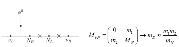
Figure 1: Dirac neutrino mass with a Dirac singlet fermion insertion.

Before going further, we should note that $\chi^{*}$ has a lepton number $L=-1$ and it is the antiparticle of $\chi$ with $L=+1$. Since CP is conserved, the transition amplitude ($M_{\chi^{*}}$) involving $\chi^{*}$ is the same as the transition amplitude ($M_{\chi}$) with $\chi$. Now let $n_{\chi}$ and $n_{\chi^{*}}$ be the number density of the particle $\chi$ and the antiparticle $\chi^{*}$, respectively. Their sum is total number density of DM, $n=n_{\chi}+n_{\chi^{*}}$. Both $\chi$ and $\chi^{*}$ make equal amount of contributions to the annihilation cross section and the CDM relic density.

III Direct Search for Leptonic Scalar Dark Matter

It is an opportune time to investigate direct detection for WIMP dark matter. The XENON1T collaboration recently announced the observation of low energy excess electronic recoil events in their detector Aprile:2020tmw . In this section, we focus on the search for nuclear recoils generated by the WIMP-nucleon scattering. We evaluate $\chi$-nucleon elastic scattering cross section for the leptonic scalar dark matter ($\chi$). In addition, we place limits on the relevant parameters $\lambda_{01}$ and $m_{\chi}$ with XENON1T results.

III.1 The Elastic Scattering of DM with Nucleus ${\cal N}$

In the LSDM model, the leptonic scalar DM ($\chi$) interacts with quarks ($q$) through the SM Higgs boson ($H$). Hence the effective Lagrangian of $\chi$ with quarks is simply

$${\cal L}_{\rm eff}=\sum_{q}a_{q}[\chi\chi^{*}][{\bar{q}}q]\,,\qquad{\rm with}\quad a_{q}\simeq\lambda_{01}\frac{m_{q}}{m_{H}^{2}}\,,$$ (8)

where $m_{q}$ and $m_{H}$ are masses of the quark and the Higgs boson, respectively, and $a_{q}$ is the effective coupling of DM interacting with the quark in a nucleon.

Before making an estimate for the detection rate of the leptonic dark matter ($\chi$) in the XENON1T experiment, let us evaluate the normalized spin independent (SI) cross section for the leptonic scalar DM scattered off the ${}^{129,131}{\rm Xe}$ nuclei. Applying the effective Lagrangian in Eq. (8), we obtain the matrix element for elastic scattering of the DM particle ($\chi$) and the nucleus (${\cal N}$) as

$$M_{fi}=2m_{\cal N}\sum_{q}a_{q}\langle{\cal N}_{f}|{\bar{q}}q|{\cal N}\rangle\,.$$ (9)

In general, the averaged unpolarized amplitude square at $q^{2}=0$ can be written as

$$\overline{\sum}|M_{fi}|^{2}(q^{2}=0) = \overline{\sum}|M^{SI}_{fi}|^{2}(q^{2}=0)+\overline{\sum}|M^{SD}_{fi}|^{2}(q^{2}=0)$$ (10)

$$= 4m_{\cal N}^{2}f^{2}_{s\cal N}\,,$$

where $SI$ and $SD$ denote the spin independent and the spin dependent contributions, respectively.

For the effective scalar interaction, we have

$$f_{s\cal N}=Zf_{sp}+(A-Z)f_{sn},$$ (11)

where

$$f_{sp(n)}=\sum_{q=u,d,s}a_{q}\frac{m_{p(n)}}{m_{q}}f^{(p(n))}_{Tq}+\sum_{q=c,b,t}a_{q}\frac{2}{27}\frac{m_{p(n)}}{m_{q}}\left(1-\sum_{q^{\prime}=u,d,s}f^{p(n)}_{Tq^{\prime}}\right)\,.$$ (12)

When evaluating the quark operator matrix element in the nuclear state, we need to include loop contributions involving heavy quarks that contribute to the mass of the nucleon ($m_{p(n)}$).

The proton mass fraction $f^{p}_{Tq}$ is defined by the matrix elements of the quark current

$$\langle p|m_{q}{\bar{q}}q|p\rangle=\left\{\begin{array}[]{lr}m_{p}f^{p}_{Tq},&q=u,d,s\,,\\ \frac{2}{27}m_{p}\left(1-\sum_{q=u,d,s}f^{p}_{Tq}\right),&q=c,b,t\,.\end{array}\right.$$ (15)

The neutron mass fraction $f^{n}_{Tq}$ is defined in the same way. The matrix elements of the light-quark currents in the proton or neutron are obtained in chiral perturbation theory from measurements of the pion-nucleon sigma term Cheng1 ; Cheng2 ; GLS ; Alarcon2011 ; Alarcon2012 ; Cheng3 . The heavy quark contribution to the mass of the nucleon is through the triangle diagram SVZ .

In the center of mass (CM) frame, the differential cross section is

$$\frac{d\sigma(\vec{q}=0)}{d|{\bf q}|^{2}}=\frac{1}{64\pi s\mu^{2}_{\cal N}v^{2}}\overline{\sum}|M_{fi}|^{2}(q^{2}=0)\,,$$ (16)

where $v$ is the DM velocity relative to the target, $\sqrt{s}\approx m_{\chi}+m_{\cal N}$ is the total energy, and $\mu_{\cal N}$ is the reduced mass of DM and the target nucleus $\cal N$. The total cross section at zero momentum transfer JKG can then be obtained as

$$\sigma_{0}^{SI}=\int^{4\mu^{2}_{\cal N}v^{2}}_{0}d|{\bf q}|^{2}\frac{d\sigma(\vec{q}=0)}{d|{\bf q}|^{2}}=\frac{\mu_{\cal N}^{2}}{\pi}f^{2}_{s\cal N}\,.$$ (17)

Hence the total cross section of DM-nucleus ($\chi-{\cal N}$) scattering becomes

$$\sigma_{{\cal N}}=\frac{\sigma^{SI}_{0}}{4\mu^{2}_{{\cal N}}v^{2}}\int^{4\mu^{2}_{{\cal N}}v^{2}}_{0}d|{\bf q}|^{2}F^{2}_{SI}(|{\bf q}|)$$ (18)

where $F^{2}_{SI}(|{\bf q}|)$ is the spin-independent form factor. To compare with the experimental results, we define the scaled SI and SD cross sections, respectively, for the nucleus with atomic mass number $A_{i}$ and isotope abundance $\eta_{i}$ as the following

$$\sigma^{SI}_{\chi p} \equiv \frac{\sum_{i}\eta_{i}\sigma_{A_{i}}}{\sum_{j}\eta_{j}A^{2}_{j}\frac{\mu^{2}_{A_{j}}}{\mu^{2}_{p}}},$$ (19)

and

$$\sigma^{SD}_{\chi p,n}\equiv(\sum_{i}\eta_{i}\sigma_{A_{i}})\left(\sum_{j}\eta_{j}\frac{4\mu_{A_{j}}^{2}\langle S_{p,n}\rangle^{2}_{\rm eff}(J_{A_{j}}+1)}{3\mu_{p,n}^{2}J_{A_{j}}}\right)^{-1},$$ (20)

where $\mu_{A_{i}}$ and $\mu_{p,n}$ are the reduced masses of the DM with the target nucleus and the DM with proton or neutron, respectively. In the above, $\langle S_{p(n)}\rangle_{\rm eff}$ and ($J_{A_{j}}$) are the proton (neutron) spin expectation value (including the contributions of two-body current Menendez ) and the total angular momentum of the nucleus with atomic mass number $A_{j}$ respectively. The effective spin expectation value is defined as $\langle S_{p(n)}\rangle_{\rm eff}\equiv\langle S_{p(n)}\rangle\pm\delta a_{1}(\langle S_{p}\rangle-\langle S_{n}\rangle)/2$ and $\delta a_{1}$ is the fraction contributing to the isovector coupling ChuaWong ; Menendez .

III.2 Numerical Results for Direct Search

At present, the XENON1T experiment Xenon1T2018-SI provides the most stringent upper limits on $\sigma^{SI}$ for WIMP masses above 6 GeV. In our analysis for spin independent cross section of $\chi-{\cal N}$ scattering, we adopt the Helm form factor LS ; VKMHS used in XENON1T experiments:

$$F^{2}_{SI}(|{\bf q}|)=\bigg{(}\frac{3j_{1}(qR_{\cal N})}{qR_{\cal N}}\bigg{)}^{2}e^{(qs)^{2}}\,,$$ (21)

where the nuclear radius $R_{\cal N}=c^{2}+\frac{7}{3}\pi^{2}a^{2}-5s^{2}$ with $c=(1.23A^{1/3}-0.6)$ fm, $a=0.52$ fm and the nuclear surface thickness $s=1$ fm. We use the updated data of nucleon mass fractions from Ref. Cheng3 : $f^{p}_{Tu}=0.017$, $f^{p}_{Td}=0.023$, $f^{n}_{Tu}=0.012$, $f^{n}_{Td}=0.033$, $f^{p,n}_{Ts}=0.053$.

In the LSDM model with a scalar dark matter ($\chi$) and a light mediator ($\zeta$), there are eight free parameters as shown in Eq. (3). In our analysis, the scan is performed with the log-prior distributions for the input parameters as shown in the below:

• $m_{H}/2\leq m_{\chi}\leq 1$ TeV, such that $\chi\chi\to\zeta H$ can occur,

• $0.2$ GeV $\leq m_{\zeta}\leq 1.2$ GeV,

• $1$ GeV $\leq\mu_{12}\leq 1$ TeV, and

• $10^{-6}\leq\lambda\leq{\cal O}(1)\sim\sqrt{4\pi}$ for $\lambda=\lambda_{1},\lambda_{2},\lambda_{01}$, or $\lambda_{12}$.

Note that $\lambda_{02}$ is chosen to be $10^{-6}\leq\lambda_{02}\leq 10^{-2}$. It is constrained by the SM Higgs invisible decay width ($H\rightarrow\zeta\zeta^{*}$), i.e.

$$\Gamma(H\rightarrow\zeta\zeta^{*})=\frac{\lambda_{02}^{2}v^{2}}{16\pi m_{H}}\,.$$ (22)

Assuming that the invisible width is less than $10\%$ of the Higgs width $\Gamma_{H}\sim 4.12$ MeV Tanabashi:2018oca , we obtain the maximal value of $\lambda_{02}\sim 6.5\times 10^{-3}$. In addition, $m_{\zeta}$ must be greater than 0.2 GeV to satisfy the cosmological constraint of effective number of neutrinos, which will be discussed later.

Figure 2: (a) The spin independent cross section $\sigma^{SI}_{\chi p}$ versus $m_{\chi}$ with random sampling for DM ($\chi$) scattered off the nuclei ^129,131Xe. Also shown are the upper limit from XENON1T Xenon1T2018-SI and the neutrino background nb3 . (b) A scatter plot for the same samples projected to the the plane of ($m_{\chi},\lambda_{01}$) with the corresponding $\lambda_{01}$.

In this model, the scaled SI and SD cross sections ($\sigma^{SI}_{\chi p}$ and $\sigma^{SD}_{\chi p,n}$) depend on two parameters: (i) the mass of leptonic scalar dark matter ($m_{\chi}$), and (ii) the coupling $\lambda_{01}$. We apply the most stringent constraint from XENON1T experiment Xenon1T2018-SI with the upper limits of SI WIMP-nucleon scattering cross section. Fig. (2a) shows the spin independent cross section $\sigma^{SI}_{\chi p}$ versus $m_{\chi}$ with random sampling for DM ($\chi$) scattered off the nuclei ^129,131Xe. In addition, a scatter plot for the same samples projected to the the plane of ($m_{\chi},\lambda_{01}$) with the corresponding $\lambda_{01}$ is presented in Fig. (2b). In this figure, we show three groups of samples: (a) all samples with red “${\color[rgb]{1,0,0}\times}$” above the the upper limits of XENON1T experiment Xenon1T2018-SI are ruled out, (b) those with green “${\color[rgb]{0,1,0}\circ}$” between the upper limits of XENON1T experiment and the curve of neutrino background nb1 ; nb2 ; nb3 are allowed and could be detectable in future detectors, and (c) the samples with blue “${\color[rgb]{0,0,1}\cdot}$” below the curve of neutrino background, and they are allowed as well. However, we may not be able to distinguish the DM event from neutrino event.

IV Relic Density and Indirect Search

The matter density ($\rho$) of the Universe is often described with a relative density ($\Omega$)

$$\Omega = \frac{\rho}{\rho_{\rm c}}$$ (23)

$$\rho_{c} = \frac{3H_{0}^{2}}{8\pi G_{N}}\simeq 1.88\times 10^{-29}h^{2}\;{\rm g}/{\rm cm}^{3}$$ (24)

where $\rho_{\rm c}$ is the critical density, $G_{N}$ is Newton’s gravitational constant, and $H_{0}$ is the Hubble constant, conventionally expressed as

$$H_{0}=100h~{}{\rm km}/s/{\rm Mpc}\,,$$ (25)

and $h\simeq 0.68$ Tanabashi:2018oca .

The Planck collaboration has measured cosmological parameters with very high precision Aghanim:2018eyx . The updated cold dark matter relic density Aghanim:2018eyx is

$$\Omega_{\rm CDM}h^{2}=0.120\pm 0.001\,.$$ (26)

We can also take a conservative approach as demonstration that $\chi$ can be produced again in the late time by other cosmological mechanisms so that the relic density at the present at $3\sigma$ allowed range follows

$$\Omega_{\chi}h^{2}\leq 0.123\,.$$ (27)

This assumption also includes the standard scenario $\Omega_{\chi}h^{2}\approx 0.12$.

IV.1 Thermal Relic Dark Matter Density

In the early Universe, DM $\chi$ existed abundantly in thermal equilibrium with other particles. The evolution of the total number density ($n(t)=n_{\chi}+n_{\chi^{*}}=2n_{\chi}$) for the leptonic dark matter is described by the Boltzmann equation:

$$\frac{dn}{dt}+3Hn=-\langle\sigma_{\mathrm{ann}}v\rangle[n^{2}-n^{2}_{\mathrm{E}}]\,,$$ (28)

where $n_{\mathrm{E}}$ is the number density at thermal equilibrium, the Hubble parameter is

$$H=\sqrt{4\pi^{3}g_{*}(T)\,T^{4}/(45M_{\mathrm{Pl}}^{2})}\simeq 1.66g_{*}^{1/2}T^{2}/M_{\mathrm{Pl}}\,,$$ (29)

$M_{\mathrm{Pl}}=1.2\times 10^{19}$ GeV is the Planck mass, $g_{*}$ is the total effective number of relativistic degrees of freedom Kolb ; CR:03 , $\langle\sigma_{\mathrm{ann}}v\rangle$ is the thermally averaged annihilation cross section times velocity, and $v$ is the relative velocity. The relative velocity

$$v\equiv v_{\rm lab}=\sqrt{s(s-4m_{\chi}^{2})}/(s-2m_{\chi}^{2})$$ (30)

and the Mandelstam variable $s=2m_{\chi}^{2}(1+1/\sqrt{1-v^{2})}$ are measured in the lab frame.

The thermally averaged annihilation cross section times velocity $\langle\sigma_{\mathrm{ann}}v\rangle$ is evaluated with the Maxwell velocity distribution,

$$\langle\sigma_{\mathrm{ann}}v\rangle = \frac{3\sqrt{6}}{\sqrt{\pi}v_{0}^{3}}\int_{0}^{\infty}dv\,v^{2}\frac{(\sigma_{\mathrm{ann}}v)_{\chi\chi^{*}}}{2}e^{-3v^{2}/2v_{0}^{2}}$$ (31)

$$= \frac{x_{f}^{3/2}}{2\sqrt{\pi}}\sum_{\varphi_{1},\varphi_{2}}\int_{0}^{\infty}dv\,v^{2}\frac{[\sigma_{\mathrm{ann}}(\chi\chi^{*}\to\varphi_{1}\varphi_{2})v]}{2}e^{-xv^{2}/4}$$

$$\quad\quad\times\theta[2m_{\chi}^{2}(1+\frac{1}{\sqrt{1-v^{2}}})-(m_{\varphi_{1}}+m_{\varphi_{2}})^{2}]\,,$$

where $x_{f}\equiv m_{\chi}/T_{f}$, $v_{0}\equiv\langle v^{2}\rangle^{1/2}=\sqrt{6/x_{f}}$ with the freeze-out temperature $T_{f}$. The second expression represents the leading contribution of DM annihilating to a pair of particles ($\varphi_{1}$ and $\varphi_{2}$) in the final state. Fig. 3 shows the Feynman diagrams for the dominant leptonic scalar DM annihilation processes. For each annihilation channel, we have put a step function ($\theta$) for the threshold energy.

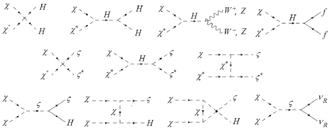
Figure 3: Feynman diagrams for leptonic scalar DM annihilation.

As the Universe cooled down, deviation of number density ($n_{\chi}$) from thermal equilibrium would begin when the temperature reached the freeze-out temperature ($T_{f}$). After the temperature dropped to approximately $T_{f}/5$, the annihilation rate of the WIMP dark matter became equal to the expansion rate of universe JKG , namely $n_{\chi}\langle\sigma_{\mathrm{ann}}v\rangle=H$. The relic mass density becomes

$$\Omega_{\chi}h^{2}=n_{\chi}m_{\chi}/\rho_{\rm c}=\frac{Hm_{\chi}}{\langle\sigma_{\mathrm{ann}}v\rangle\rho_{\rm c}}$$ (32)

and the leptonic scalar $\chi$ remains as cold dark matter. From the freeze-out condition, $n_{\chi}\langle\sigma_{\mathrm{ann}}v\rangle=H$, the freeze-out temperature parameter $x_{f}$ can be solved numerically by the following equation Kolb ; JKG

$$x_{f}={\rm ln}\left[c(c+2)\sqrt{\frac{45}{8}}\frac{g_{\chi}m_{\chi}M_{\rm pl}(a+6b/x_{f})}{2\pi^{3}\sqrt{g_{*}(m_{\chi}/x_{f})}x_{f}^{1/2}}\right]\,.$$ (33)

In the above, $c$ is an order of unity parameter determined by matching the late-time and early-time in the freeze-out criterion. The exact value of $c$ is not so significant to solve the numerical solution for $x_{f}$ due to the logarithmic dependence in Eq. (33). Following the standard procedure Kolb to solve the Boltzmann equation [Eq.(28)], the relic DM density $\Omega_{\rm DM}\equiv\rho_{\chi}/\rho_{\rm c}$ can be approximately related to $\langle\sigma_{\rm ann}v\rangle$ as

$$\Omega_{\text{DM}}h^{2}\approx 1.04\times 10^{9}\frac{{\rm GeV}^{-1}}{M_{\mathrm{Pl}}\sqrt{g_{*}\left(T_{f}\right)}J(x_{f})},$$ (34)

where

$$J\left(x_{f}\right)\equiv\int_{x_{f}}^{\infty}\frac{\langle\sigma_{\mathrm{ann}}v\rangle}{x^{2}}dx=\int_{0}^{\infty}dv\frac{(\sigma_{\rm ann}v)_{\chi\chi^{*}}}{2}v\left[1-{\rm erf}\left(v\sqrt{x}_{f}/2\right)\right].$$ (35)

In the non-relativistic limit, $J(x_{f})=a/x_{f}+3b/x_{f}^{2}$.

The DM particles became non-relativistic (NR) when they froze out of thermal equilibrium in the early universe. In the NR limit, we have $\sigma_{\mathrm{ann}}(\chi\chi^{*}\rightarrow{\rm all})v=a+bv^{2}+O(v^{4})$ by applying the Taylor series expansion and its thermally-averaged value Eq. (31) can be simplified as $\langle\sigma_{\mathrm{ann}}v\rangle=a+6b/x_{f}+O(1/x_{f}^{2})$.

IV.2 Indirect Search for Leptonic Scalar Dark Matter

In the halo of the Milky Way and nearby galaxies, WIMP DM annihilation might generate high energy gamma-rays and appear in detectors such as Fermi-LAT Fermi-LAT2015 ; Fermi-LAT:2016uux , H.E.S.S. HESS2016 ; Rinchiuso:2019rrh , HAWC Albert:2017vtb , MAGIC Ahnen:2017pqx , or VERITAS Archambault:2017wyh . In addition, WIMP dark matter would lose energy when they pass through massive stars such as the sun. They become gravitationally trapped and accumulate. WIMP annihilations could be sources of high energy neutrinos and might be detected by ANTARES ANTARES:2019svn and IceCube Aartsen:2020tdl .

At present, the most stringent limits for our surveyed DM mass range, $m_{H}/2<m_{\chi}<1000$ GeV, come from Fermi-LAT Fermi-LAT2015 ; Fermi-LAT:2016uux and H.E.S.S. HESS2016 . We will evaluate the leptonic scalar DM annihilation cross section $\langle\sigma_{\rm ann}v\rangle$ in different channels, and investigate the discovery potential as well as determine favored parameters guided by the Fermi-LAT and the H.E.S.S. data.

Fermi-LAT analyzed 15 dwarf spheroidal satellite galaxies (dSphs) Fermi-LAT2015 ; Fermi-LAT:2016uux , while the H.E.S.S observed $\gamma$-ray towards the inner 300 parsecs of the Milky Way. The speed of the sun moving around the galactic center is approximately 220 km/s at the local distance $r\approx$ 8.5 kpc and the galactic circular rotation speed is about 230 km/s at radii $\approx$ 100 kpc JKG ; Kochanek:1995xv . On the other hand, the distance between the 15 dSphs and the sun is $\approx 23--233$ kpc Fermi-LAT2015 . In the indirect-detection calculation, we conventionally adopt a typical DM velocity $v_{0}\simeq 10^{-3}$ in the unit of the light speed Ferrer:2013cla .

In the leptonic scalar DM model, the dark matter particle ($\chi$) can annihilate into a pair of SM particles such as $W^{+}W^{-}$, $Z^{0}Z^{0}$, $HH$, fermion pairs $f\bar{f}$, or $\zeta\zeta^{*}$ through s-channel exchange of SM Higgs boson $H$. In addition, The leptonic scalar DM can also annihilate into a pair of $\zeta\zeta^{*}$ or $HH$ through 4-point interactions and t-channel exchange of $\chi$, or $\nu_{R}\nu_{R}$ through s-channel exchange of $\zeta$, or a pair of $\zeta H$ through s-exchange of $\zeta$ and t- and u-channel exchange of $\chi$ as presented in Fig. 3. From these Feynman diagrams, we calculate the corresponding DM annihilation cross sections at tree-level:

$$(\sigma v)_{\chi\chi^{*}\rightarrow\zeta\zeta^{*}} = \frac{\sqrt{s-4m_{\zeta}^{2}}}{16\pi\sqrt{s}(s-2m_{\chi}^{2})}\left\{\lambda_{12}^{2}+\frac{16\mu_{12}^{2}}{m_{\zeta}^{4}-m_{\chi}^{2}(s-4m_{\zeta}^{2})}\right.$$ (36)

$$\quad\quad+\frac{\lambda_{01}^{2}\lambda_{02}^{2}v^{4}-2\lambda_{01}\lambda_{02}\lambda_{12}v^{2}(s-m_{H}^{2})}{(s-m_{H}^{2})^{2}+m_{H}^{2}\Gamma_{H}^{2}}$$

$$\quad\quad+\frac{8\mu_{12}^{2}\left[\lambda_{12}\left((s-mH^{2})^{2}+m_{H}^{2}\Gamma_{H}^{2})-\lambda_{01}\lambda_{02}v^{2}(s-M_{H}^{2}\right)\right]}{\sqrt{(s-4m_{\chi}^{2})(s-4m_{\zeta}^{2})}\left((s-mH^{2})^{2}+m_{H}^{2}\Gamma_{H}^{2}\right)}$$

$$\left.\quad\quad\times\log\left[\frac{s-2m_{\zeta}^{2}+\sqrt{(s-4m_{\chi}^{2})(s-4m_{\zeta}^{2})}}{s-2m_{\zeta}^{2}-\sqrt{(s-4m_{\chi}^{2})(s-4m_{\zeta}^{2})}}\right]\right\},$$

$$(\sigma v)_{\chi\chi^{*}\rightarrow f\bar{f}}=\frac{\mathcal{C}_{f}\lambda_{01}^{2}m_{f}^{2}(s-4m_{f}^{2})^{3/2}}{8\pi\sqrt{s}(s-2m_{\chi}^{2})[(s-m_{H}^{2})^{2}+m_{H}^{2}\Gamma_{H}^{2}]},$$ (37)

$$(\sigma v)_{\chi\chi^{*}\rightarrow VV}=\frac{\lambda_{01}^{2}\sqrt{s-4m_{V}^{2}}(s^{2}-4sm_{V}^{2}+12m_{V}^{4})}{16\pi\sqrt{s}(s-2m_{\chi})[(s-m_{H}^{2})^{2}+m_{H}^{2}\Gamma_{H}^{2}]}{S},\quad{S}=\left\{\begin{array}[]{rcl}1&\mbox{for}&W^{+}W^{-}\\ 1/2&\mbox{for}&\ Z^{0}Z^{0}\end{array}\right.$$ (40)

$$(\sigma v)_{\chi\chi\rightarrow\nu_{Ri}\nu_{Rj}}=\frac{\mu_{12}^{2}|f_{ij}|^{2}\sqrt{s-4m_{\nu}^{2}}(s-2m_{\nu}^{2})}{\pi\sqrt{s}(s-2m_{\chi}^{2})[(s-m_{\zeta}^{2})^{2}+m_{\zeta}^{2}\Gamma_{\zeta}^{2}]},$$ (41)

$$(\sigma v)_{\chi\chi\rightarrow\zeta H}=\frac{(\lambda_{01}\mu_{12}v)^{2}\sqrt{A}}{2\pi(s-2m_{\chi}^{2})(m_{\chi}^{2}A+sm_{H}^{2}m_{\zeta}^{2})}+\frac{2(\lambda_{01}\mu_{12}v)^{2}s\tanh^{-1}(\sqrt{AB}/{C})}{\pi(s-2m_{\chi}^{2})\sqrt{B}C}$$

$$\qquad\qquad\qquad-\frac{2\lambda_{01}\lambda_{02}(\mu_{12}v)^{2}(s-m_{\zeta}^{2})\tanh^{-1}(\sqrt{AB}/{C})}{\pi(s-2m_{\chi}^{2})\sqrt{B}D}+\frac{(\lambda_{02}\mu_{12}v)^{2}\sqrt{A}}{4\pi s(s-2m_{\chi}^{2})D},$$ (42)

where

$$A = [s-(m_{H}+m_{\zeta})^{2}][s-(m_{H}-m_{\zeta})^{2}],$$

$$B = s(s-4m_{\chi}^{2}),$$

$$C = s(s-m_{H}^{2}-m_{\zeta}^{2}),$$

$$D = (s-m_{\zeta}^{2})^{2}+m_{\zeta}^{2}\Gamma_{\zeta}^{2}.$$ (43)

After substituting $s=2m_{\chi}^{2}(1+1/\sqrt{1-v^{2}})$ into the above equations and expanding around $v^{2}$, one can obtain the usual form: $\langle\sigma_{\mathrm{ann}}v\rangle=\langle a+bv^{2}+{\cal O}(v^{4})\rangle$ in the non-relativistic limit. As discussed in Sec. II, the decay lifetime of $\zeta$ is so short that the $\zeta$ has all decayed into two right-handed neutrinos $\nu_{R}$, and the light $\nu_{R}$ decouples from the SM particles at its freeze out temperature $T^{R}_{f}\sim m_{\zeta}$ before the onset of BBN.

IV.3 Sommerfeld Enhancement Effect

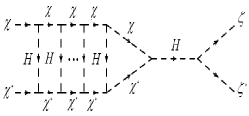
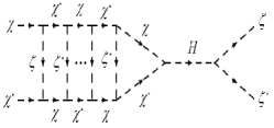
Figure 4: Schematic diagrams for non-pertubative annihilation processes: $\chi\chi^{*}\rightarrow\zeta\zeta^{*}$ and $\chi\chi^{*}\rightarrow\nu_{R}\nu_{R}$.

When the DM particles froze out in the early universe, they became non-relativistic and the non-perturbative Sommerfeld enhancement effect becomes important Hisano:2004 ; Hisano:2005 ; Hisano:2006nn ; AFSW ; Chun1 ; Chun2 ; Chun3 . We present the schematic diagrams of annihilation processes with the Sommerfeld enhancement effect for $\chi\chi^{*}\rightarrow\zeta\zeta^{*}$ in Figs. 4(a,b) and for $\chi\chi\rightarrow\nu_{R}\nu_{R}$ in Figs. 4(c). In fact, Sommerfeld effect contains an infinite series of the ladder diagrams.

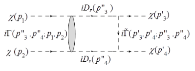
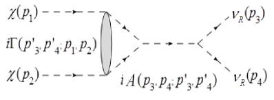
Figure 5: Diagrams for (a) rescattering of $\chi\chi\to\chi\chi$, and (b) nonperturbative annihilation of $\chi\chi\to\nu_{R}\nu_{R}$.

Let us first consider the easier case of Sommerfeld enhancement effect on the annihilation process $\chi(p_{1})\chi(p_{2})\to\nu_{R}(p_{3})\nu_{R}(p_{4})$ through the exchange of the mediator $X=H$, as shown in Fig. 4(c). When DM particles $\chi\chi$ become non-relativistic, they rescatter off each other [Fig. 5(a)] before annihilating to $\nu_{R}\nu_{R}$. The Sommerfeld enhanced amplitude $iA_{S}$ of $\chi\chi\to\nu_{R}\nu_{R}$ annihilation process [Fig. 5(b)] can be expressed as

$$iA_{\mathcal{S}}(p_{3},p_{4},p_{1},p_{2}) = iA(p_{3},p_{4},p_{1},p_{2})$$ (44)

$$+ \int\frac{d^{4}p^{\prime}_{3}}{(2\pi)^{4}}iA(p_{3},p_{4};p^{\prime}_{3},p^{\prime}_{4})(iD_{F}(p^{\prime}_{3}))i\Gamma(p^{\prime}_{3},p^{\prime}_{4};p_{1},p_{2})(iD_{F}(p^{\prime}_{4})),$$

where $iA$ is the amplitude of the annihilation process at tree level, $D_{F}$ is the leptonic scalar DM propagator and $i\Gamma$ is the amputated non-perturbative 4-point vertex function [Fig. 5(a)] describing the rescattering process of $\chi(p_{1})\chi(p_{2})\to\chi(p^{\prime}_{3})\chi(p^{\prime}_{4})$ and satisfying the following equation:

$$i\Gamma(p^{\prime}_{3},p^{\prime}_{4},p_{1},p_{2}) = i\tilde{\Gamma}(p^{\prime}_{3},p^{\prime}_{4};p_{1},p_{2})$$ (45)

$$+ \int\frac{d^{4}p^{\prime\prime}_{3}}{(2\pi)^{4}}i\tilde{\Gamma}(p^{\prime}_{3},p^{\prime}_{4};p^{\prime\prime}_{3},p^{\prime\prime}_{4})\left[iD_{F}(p^{\prime\prime}_{3})\right]i\Gamma(p_{1},p_{2};p^{\prime\prime}_{3},p^{\prime\prime}_{4})\left[iD_{F}(p^{\prime\prime}_{4})\right].$$

In the above, we have the lowest order perturbative 4-point vertex function given by

$$i\tilde{\Gamma}(p^{\prime}_{3},p^{\prime}_{4};p^{\prime\prime}_{3},p^{\prime\prime}_{4})=-ig_{X}^{2}\frac{1}{(p^{\prime\prime}_{3}-p^{\prime}_{3})^{2}-m^{2}_{X}},$$ (46)

where $X$ is the mediator particle ($X=H$), and $p^{\prime\prime}_{4}=-p^{\prime\prime}_{3}+p^{\prime}_{3}+p^{\prime}_{4}$. Note that the dimensionless coupling strength of DM $\chi$ with the mediator $X$ is $g_{X}=g^{\prime}_{X}/(2m_{\chi})$, where the dimensionful coupling $g^{\prime}_{X}$ is usually defined in the interaction Lagrangian. When the process is mediated by the Higgs boson ($H$), we have $g_{H}=g^{\prime}_{H}/(2m_{\chi})=\lambda_{01}{\rm v}/(2m_{\chi})$, where the dimensionful coupling $g^{\prime}_{H}=\lambda_{01}{\rm v}$ as described in the scalar potential [Eq. (1)].

Form Appendix A.1, we find that the pair of DM particles $\chi\chi$ form a bound state and the wave function $\psi(\vec{r})$ satisfies the following Schrödinger equation:

$$-\frac{1}{2\mu}\nabla^{2}\psi(\vec{r})+V(\vec{r})\psi(\vec{r})=E\psi(\vec{r})=\frac{1}{2}\mu v^{2}\psi(\vec{r})\,.$$ (47)

where $\mu=m_{\chi}/2$ is the reduce mass of the bound state ($\chi\chi$), and $E=|\vec{p}|^{2}/2\mu\equiv\mu v^{2}/2$ is the total kinetic energy with the relative velocity $v=v_{\rm lab}$ defined in Eq. (30). $V(r)$ is a Yukawa-type potential

$$V(r)=-\alpha_{X}\frac{e^{-m_{X}r}}{r},$$ (48)

where $\alpha_{X}=g_{X}^{2}/4\pi$ and $m_{X}$ is the mass of mediator.

For the case of s-wave rescattering, the Sommerfeld enhanced amplitude $iA_{\mathcal{S}}$ can be written as

$$iA_{\mathcal{S}}(p_{1},p_{2};p_{3},p_{4})=iA(\vec{p}_{1},\vec{p}_{2};\vec{p}_{3},\vec{p}_{4})\psi(\vec{r}=0),$$ (49)

where $iA$ is the amplitude at tree level as explained in Appendix A.2. Consequently, the Sommerfeld enhanced velocity averaged annihilation cross section $\langle\sigma v\rangle_{\mathcal{S}}\simeq a_{\mathcal{S}}+b_{\mathcal{S}}v^{2}$ can be further simplified as

$$\langle\sigma v\rangle_{\mathcal{S}}\sim a_{\mathcal{S}}=\langle a\mathcal{S}(v)\rangle\,,\quad\mathcal{\mathcal{S}}=|\psi_{l=0}(\vec{r}=0)|^{2},$$ (50)

where $\mathcal{S}$ is just the s-wave Sommerfeld enhancement factor (see Appendix A.2).

It is well known that there is no analytical solution with a Yukawa potential in Eq. (47), but the Hulthén potential maintains the same short and long distance behavior of the Yukawa potential and has an analytical solution for s-wave function. Hence it is a good approximation to employ the Hulthén potential to obtain $|\psi_{l=0}(\vec{r}=0)|$ with a Yukawa potential Cassel ,

$$V(\vec{r})\simeq-\alpha_{X}\frac{(\pi^{2}m_{X}/6)e^{-\pi^{2}m_{X}r/6}}{1-e^{-\pi^{2}m_{X}r/6}}\,,$$ (51)

where the mediator particle $X=H$. One can obtain the wave function ChuaWong2017 in terms of Gamma function $\Gamma$

$$\psi_{l=0}(\vec{r}=0) = i\frac{\pi^{2}\epsilon_{X}/6}{2\epsilon_{v}}\,\Gamma\left(1-i\frac{\epsilon_{v}}{\pi^{2}\epsilon_{X}/6}\left(1+\sqrt{1-\frac{\pi^{2}\epsilon_{X}/6}{\epsilon^{2}_{v}}}\right)\right)$$ (52)

$$\times\Gamma\left(1-i\frac{\epsilon_{v}}{\pi^{2}\epsilon_{X}/6}\left(1-\sqrt{1-\frac{\pi^{2}\epsilon_{X}/6}{\epsilon^{2}_{v}}}\right)\right)\bigg{/}\Gamma\left(\frac{-2i\epsilon_{v}}{\pi^{2}\epsilon_{X}/6}\right),$$

with 

$$\epsilon_{v}\equiv\frac{v}{2\alpha_{X}},\quad\epsilon_{X}\equiv\frac{m_{X}}{\alpha_{X}m_{\chi}},$$ (53)

and the s-wave Sommerfeld factor is given by Feng:2010zp

$$\mathcal{S}(m_{\chi},m_{X},\alpha_{X},v)=|\psi_{l=0}(\vec{r}=0)|^{2}=\frac{\pi}{\epsilon_{v}}\frac{\sinh\left(\frac{2\pi\epsilon_{v}}{\pi^{2}\epsilon_{X}/6}\right)}{\cosh\left(\frac{2\pi\epsilon_{v}}{\pi^{2}\epsilon_{X}/6}\right)-\cos\left(2\pi\sqrt{\frac{1}{\pi^{2}\epsilon_{X}/6}-\frac{\epsilon^{2}_{v}}{(\pi^{2}\epsilon_{X}/6)^{2}}}\right)}.$$ (54)

For $\chi\chi\rightarrow\nu_{R}\nu_{R}$ annihilation process, the mediator particle is $X=H$. $\psi_{l=0}(\vec{r}=0)$ indeed goes to 1 in the $\alpha_{X}=0$ limit. We will see that the analytic solution $\mathcal{S}=\psi_{l=0}(\vec{r}=0)$ agrees well with that obtained from numerically solving the Schrödinger equation with the Yukawa potential.

When the mediator mass can be neglected, the Yukawa potential can be approximated by a Coulomb potential:

$$V(r)\simeq-\frac{\alpha_{X}}{r}.$$ (55)

The corresponding s-wave function is given by Coulomb

$$\psi_{l=0}^{(coul)}(\vec{r})=\Gamma(1+i\gamma)e^{-\pi\gamma/2}e^{i\vec{p}\cdot\vec{r}}{}_{1}\mathcal{F}_{1}(-i\gamma,1,ipr-i\vec{p}\cdot\vec{r}),$$ (56)

where ${}_{1}\mathcal{F}_{1}$ is the confluent hyper-geometric function of the first kind, and

$$\gamma=\frac{\alpha_{X}}{v}=\frac{\alpha_{X}\mu}{|\vec{p}|}.$$ (57)

In this approximation we have

$$\psi_{l=0}^{(coul)}(\vec{r}=0)=\Gamma(1+i\gamma)e^{-\pi\gamma/2}.$$ (58)

Accordingly, the corresponding s-wave Sommerfeld factor in the Coulomb potential is

$$\mathcal{S}^{(coul)}=|\psi_{l=0}^{(coul)}(\vec{r}=0)|^{2}=\Gamma(1+i\gamma)\Gamma(1-i\gamma)e^{-\pi\gamma}=\frac{2\pi\gamma}{e^{2\pi\gamma}-1}.$$ (59)

In fact $|\psi_{l=0}(\vec{r}=0)|$ goes to $|\psi_{l=0}^{Coul}(\vec{r}=0)|$ and the Sommerfeld factor $\mathcal{S}$ in Eq. (54) does reduce to $\mathcal{S}^{(coul)}$ in the large $m_{\chi}$ region Cassel ; Lebedev0 .

(a) Analytical and numerical solutions.

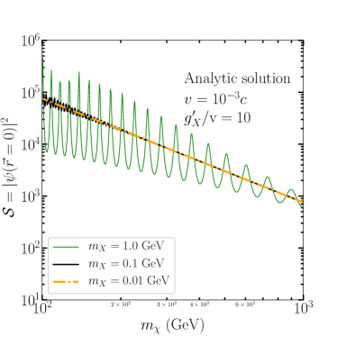
(b) Three different benchmark masses $m_{X}$.

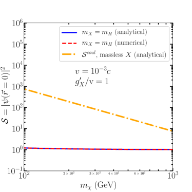
(c) Analytical and numerical solutions.

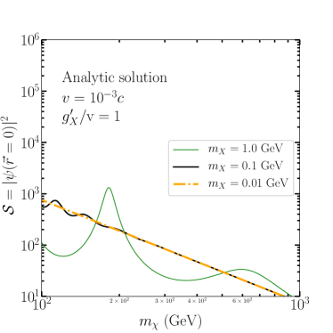
(d) Three different benchmark masses $m_{X}$.

Figure 6: Sommerfeld factor $\mathcal{S}$ versus $m_{\chi}$ for the present universe with $v=10^{-3}c$. The $g^{\prime}_{X}$ parameter is the dimensionful coupling between the DM ($\chi$) and the mediator $X$. The left panels [(a) and (c)] present the analytical results (blue solid) with the Hulthén potential [Eq. (51)] and $m_{X}=m_{H}$, as well as numerical results (red dashed) with Yukawa potential [Eq. (48)] and $m_{X}=m_{H}$. For comparison, the analytical solution in Coulomb potential approximation is depicted by orange dashed lines. In the right panels [(b) and (d)], the analytical solutions in Huthén potential approximation are shown with three values of the mediator mass $m_{X}=0.01$ (orange dot-dashed), 0.1 (black solid), and 1 $\,\mathrm{GeV}$ (green solid).

As mentioned above, we only keep the first term (the $a$ term) in Eqs.(36-42) for both relic density calculation and the indirect annihilation processes, namely, the s-wave contribution, with $\langle\sigma_{\mathrm{ann}}v\rangle\approx a+{\cal O}(v^{2})$. Hence we show the $a$-term for each annihilation process as follows:

$$a^{\zeta\zeta^{*}} = \frac{\sqrt{m_{\chi}^{2}-m_{\zeta}^{2}}}{32\pi m_{\chi}^{3}}\left\{\frac{(\mu_{12}^{2}-\lambda_{12}m_{\zeta}^{2}+2\lambda_{12}m_{\chi}^{2})^{2}}{(2m_{\chi}^{2}-m_{\zeta}^{2})^{2}}+\frac{\lambda_{01}^{2}\lambda_{02}^{2}v^{4}}{[(4m_{\chi}^{2}-m_{H}^{2})^{2}+m_{H}^{2}\Gamma_{H}^{2}]}\right.$$ (60)

$$- \left.\frac{2\lambda_{01}\lambda_{02}v^{2}(4m_{\chi}^{2}-m_{H}^{2})(4\mu_{12}^{2}-\lambda_{12}m_{\zeta}^{2}+2\lambda_{12}m_{\chi}^{2})}{(2m_{\chi}^{2}-m_{\zeta}^{2})[(4m_{\chi}^{2}-m_{H}^{2})^{2}+m_{H}^{2}\Gamma_{H}^{2}]}\right\},$$

$$a^{f\bar{f}} = \frac{C_{f}\lambda_{01}^{2}m_{f}^{2}(m_{\chi}^{2}-m_{f}^{2})^{3/2}}{4\pi m_{\chi}^{3}[(4m_{\chi}^{2}-m_{H}^{2})^{2}+m_{H}^{2}\Gamma_{H}^{2}]},$$ (61)

$$a^{VV} = \frac{\lambda_{01}^{2}\sqrt{m_{\chi}^{2}-m_{W}^{2}}(4m\chi^{4}-4m_{\chi}^{2}m_{W}^{2}+3m_{W}^{4})}{8\pi m_{\chi}^{3}((4m_{\chi}^{2}-m_{H}^{2})^{2}+m_{H}^{2}\Gamma_{H}^{2}))}{S},$$ (62)

$$a^{\nu_{Ri}\nu_{Rj}} = \frac{\mu_{12}^{2}|f_{ij}|^{2}(2m_{\chi}^{2}-m_{\nu}^{2})\sqrt{m_{\chi}^{2}-m_{\nu}^{2}}}{\pi m_{\chi}^{3}[(4m_{\chi}^{2}-m_{\zeta}^{2})^{2}+m_{\zeta}^{2}\Gamma_{\zeta}^{2}]},$$ (63)

$$a^{\zeta H} = \frac{\mu_{12}^{2}v^{2}}{128\pi m_{\chi}^{4}D}\left\{4\sqrt{A}\left[\lambda_{02}^{2}+\frac{8\lambda_{01}^{2}D(A+4m_{H}^{2}m_{\zeta}^{2})}{(A+4m_{H}^{2}m_{\zeta}^{2})^{2}}\right]\right.$$ (64)

$$- \left.\frac{128\lambda_{01}m_{\chi}^{2}\left[\lambda_{02}(4m_{\chi}^{2}-m_{\zeta}^{2})C-8\lambda_{01}m_{\chi}^{2}D\right]}{\sqrt{B}C}\right\}.$$

For $\chi\chi\to\nu_{R}\nu_{R}$ and $\zeta H$ annihilation processes, we have

$$\langle\sigma v\rangle_{\mathcal{S}}(\chi\chi\to\nu_{R}\nu_{R}) \simeq \langle a^{\nu_{R}\nu_{R}}\mathcal{S}(m_{\chi},m_{H},\alpha_{H},v)\rangle,$$ (65)

$$\langle\sigma v\rangle_{\mathcal{S}}(\chi\chi\to\zeta H) \simeq \langle a^{\zeta H}\mathcal{S}(m_{\chi},m_{H},\alpha_{H},v)\rangle.$$ (66)

Accordingly, we can analytically obtain the Sommerfeld factor $\mathcal{S}=|\psi_{l=0}(\vec{r}=0)|$ for the $\chi\chi\to\nu_{R}\nu_{R}$ and $\chi\chi\to\zeta H$ annihilation processes.

Fig. 6 shows the s-wave Sommerfeld factor in the present universe with ($v=10^{-3}c$) as a function of the DM mass ($m_{\chi}$) for two values of the coupling $g^{\prime}_{X}/{\rm v}=10$ [(a) and (b)] as well as $g^{\prime}_{X}/{\rm v}=1$ [(c) and (d)]. The left panels [(a) and (c)] present the analytical results with the Hulthén potential [Eq. (51)] and $m_{X}=m_{H}$, as well as numerical results with Yukawa potential [Eq. (48)] and $m_{X}=m_{H}$. In addition, we show the analytical solution in Coulomb potential approximation. In the right panels [(b) and (d)], the analytical solutions in Huthén potential approximation are presented with three values of the mediator mass $m_{X}=0.01,0.1$, and 1 $\,\mathrm{GeV}$. The Coulomb potential approximation in the left panels and the anlytical solution with $m_{X}=0.01\,\mathrm{GeV}$ in the right panels are both represented with orange dot-dashed lines because there is no difference between them numerically.

We find that all curves in Figs. 6(b) and 6(d) with a massive $m_{X}$ oscillate with an amplitude that increases with an increasing mediator mass, while the frequency of oscillation increases with a decreasing mediator mass. Comparing Fig. 6(a,b) and Fig. 6(c,d), we see that the Sommerfeld enhancement factor $\mathcal{S}$ decreases with a decreasing coupling $g^{\prime}_{X}$. Furthermore, the strength of Sommerfeld enhancement decreases with an increasing $m_{\chi}$. The reason can be seen as follows:

• First, these curves oscillate around the curve generated by the Coulomb potential.

• The Coulomb potential approximation provides the central value for $\mathcal{S}$.

• From Eq. (57) and Eq. (59), we note that $\mathcal{S}^{(coul)}$ is a function of $\alpha_{X}=g^{2}_{X}/{4\pi}$. Hence the enhancement factor $\mathcal{S}$ is suppressed by an increasing $m_{\chi}$ owing to $g_{X}=g^{\prime}_{X}/m_{\chi}$.

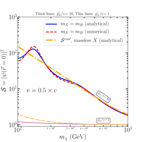
Figure 7: Sommerfeld factor $\mathcal{S}$ versus $m_{\chi}$ for the early universe with $v=0.5\times c$. The color scheme is same as Fig. 6. The coupling $g^{\prime}_{X}/{\rm v}$ for the upper thick lines are fixed to $10$ while the value of the bottom thin lines are $1$.

In Fig. 7, we show $\mathcal{S}$ at the early universe with $(v=0.5\times c)$ as a function of $m_{\chi}$. The colored scheme is the same as Fig. 6 while the thick and thin lines are based on $g^{\prime}_{X}/{\rm v}=10$ and $g^{\prime}_{X}/{\rm v}=1$, respectively. Clearly, comparing with low-velocity DM in present universe as shown in Fig. 6, the nonperturbative effect for high-velocity becomes much weaker resulting in much smaller Sommerfeld enhancement in the early universe.

From Fig. 6 and Fig. 7, we find that, the larger coupling strength or smaller DM relative velocity $v$ gives a greater value of the Sommerfeld factor. Roughly speaking, the Sommerfeld factor used at the present stage ($v\simeq 10^{-3}c$) is 2$\sim$3 order of magnitude greater than that in freeze-out stage $(v\simeq 0.5\times c)$ with a light mediator mass. This main characteristics of velocity dependent SICS is used to solve the small scale problem.

We have shown in Fig. 6 and Fig. 7 that the numerical result agrees well with the analytic solution in Hulthén approximation at $m_{X}=m_{H}$. Nevertheless, we see that it is impossible to obtain an analytical form for $\mathcal{S}$ in the process of $\chi\chi^{*}\to\chi^{*}\chi$, which simultaneously involves the exchanges of $H$ and $\zeta$ particles schematically shown in Fig. 4(a,b). The potential then becomes the sum of two Yukawa-type potential

$$V(r)=-\alpha_{H}\frac{e^{-m_{H}r}}{r}-\alpha_{\zeta}\frac{e^{-m_{\zeta}r}}{r}.$$ (67)

where $\alpha_{X}={g_{X}^{2}}/{4\pi},(X=H,\zeta)$, $g_{H}={\lambda_{01}{\rm v}}/{2m_{\chi}}$ and $g_{\zeta}={\mu_{12}}/{m_{\chi}}$. There is no analytical form for the Sommerfeld enhancement factor $\mathcal{S}$. Therefore, we develop a numerical solution for $\mathcal{S}$ as given in Appendix A.3.

IV.4 Numerical Results for Relic Density and Indirect Search

In this subsection, we present our numerical results for the indirect search and the relic density. For the indirect search, we compare our theoretical results with the most stringent limits from the Fermi-LAT Fermi-LAT2015 ; Fermi-LAT:2016uux and the H.E.S.S. results HESS2016 . Both Fermi-LAT and H.E.S.S. astrophysical observations do not show the significant $\gamma$-ray signal above background. Instead, Fermi-LAT provides upper limits on $\langle\sigma_{\rm ann}v\rangle$ for DM annihilating into $W^{+}W^{-}$ and the SM fermion pairs: $b{\bar{b}},u{\bar{u}},\tau^{+}\tau^{-},\mu^{+}\mu^{-},e^{+}e^{-}$ at $95\%$ confidence level with WIMPs masses between 2 GeV to 10 TeV, while H.E.S.S. gives the upper limits on $\langle\sigma_{\rm ann}v\rangle$ for DM annihilating into $W^{+}W^{-}$ and the SM fermion pairs: $t{\bar{t}},b{\bar{b}},\tau^{+}\tau^{-},\mu^{+}\mu^{-}$ with masses from 160 GeV to 70 TeV.

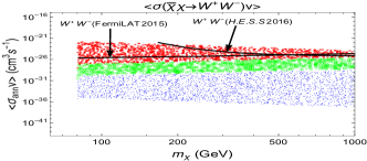
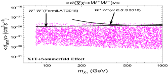
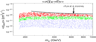
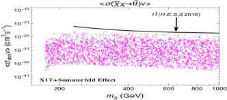
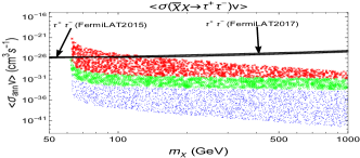
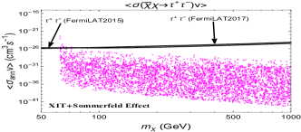
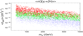
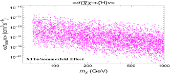
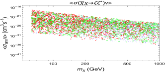
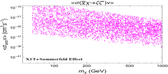
Figure 8: Thermally averaged annihilation cross section times velocity for the leptonic scalar dark matter ($\chi$) $\langle\sigma_{\rm ann}v\rangle$ in different channels. [Left] Without the Sommerfeld effect: red “${\color[rgb]{1,0,0}\times}$”, green “${\color[rgb]{0,1,0}\circ}$” and blue “${\color[rgb]{0,0,1}\cdot}$” denote the scenario excluded by XENON1T, testable soon by future underground detectors, and below the neutrino floor, respectively. [Right] the Sommerfeld effect for those samples surviving from XENON1T limit, namely green “${\color[rgb]{0,1,0}\circ}$” and blue “${\color[rgb]{0,0,1}\cdot}$” in the left panels.

Fig. 8 presents $\langle\sigma_{\rm ann}v\rangle$ for leptonic scalar DM ($\chi\chi$) annihilating into $W^{+}W^{-}$, $t\bar{t}$, $\tau^{+}\tau^{-}$, $\zeta H$ and $\zeta\zeta^{*}$. The samples above the upper limits of Fermi-LAT and H.E.S.S are ruled out. The plots on the left-handed do not include the Sommerfeld effect but the Sommerfeld effect are considered in the plots on the right-handed side. In each plot on the left-handed side, the same color scheme as presented in Fig. 2 is used. In the panels of the right column, we show the Sommerfeld effect for the data survived from XENON1T limits, namely the samples taken from those green “${\color[rgb]{0,1,0}\circ}$” and blue “${\color[rgb]{0,0,1}\cdot}$” in the left panels.

Without considering the Sommerfeld effect, we see that DM can only be detected with $m_{\chi}\gtrsim 1$ TeV via $W^{+}W^{-}$ or the Higgs resonance annihilation via $b\bar{b}$ and $\tau^{+}\tau^{-}$ channel. Clearly, the cross sections can be enhanced by the Sommerfeld effect. Albeit the enhancement differs from channel to channel, it is interesting that the cross section of the channel $\zeta\zeta^{*}$ is overall enhanced. We see that DM annihilating to a pair of $\zeta\zeta^{*}$ is dominant while this channel is not detectable because $\zeta$ eventually decays to $\nu_{R}$.

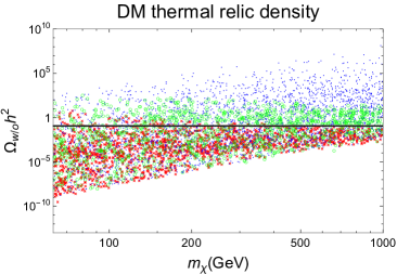
(a)  Sommerfeld effect not included

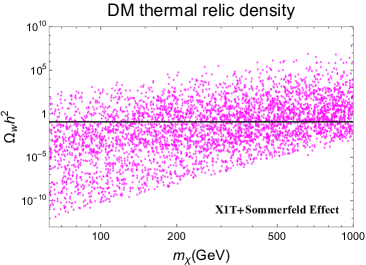
(b)  Sommerfeld effect included

Figure 9: Relic density of leptonic scalar DM $\Omega_{\chi}h^{2}$ versus $m_{\chi}$: (a) without Sommerfeld enhancement, and (b) with Sommerfeld enhancement.

Fig. 9 shows the leptonic scalar DM thermal relic density $\Omega_{\chi}h^{2}$ as a function of $m_{\chi}$: (a) without Sommerfeld enhancement, and (b) with Sommerfeld enhancement effects. We maintain the same symbols for each sample used in Fig. 2 and Fig. 8. The horizontal line denotes the observed relic density: $\Omega_{\rm obs}h^{2}=0.120$ Tanabashi:2018oca . Since the relic density is roughly proportional to the inverse of the total $\langle\sigma_{\rm ann}v\rangle$, the samples are oriented reversely in vertical direction. With Sommerfeld enhancement effect, the same parameters will lead to a smaller relic density as expected. Thus, there are more regions of the parameter space satisfying the relic density requirement $\Omega_{\chi}h^{2}<0.123$ Tanabashi:2018oca .

V Cosmological Constraints on the Right-handed Neutrino

The left-handed neutrino decouple at the temperature $T_{f}^{L}\sim 1$ MeV when the left-handed neutrinos and the right-handed anti-neutrinos can not been converted to pairs of electron and positron. On the other hand, the right-handed neutrinos decouple at the temperature $T_{f}^{R}\sim m_{\zeta}$ when the production of the $\zeta$ particles is kinetically not allowed. At the temperature $T<T_{f}^{L}<T_{f}^{R}$, the total density of radiation $\rho_{r}$ is

$$\rho_{r}=\rho_{\gamma}+\rho_{L}+\rho_{R}=3\Bigl{[}1+N_{\rm eff}\frac{7}{8}(\frac{4}{11})^{4/3}\Bigr{]}\rho_{\gamma},$$ (68)

where $\rho_{\gamma}$, $\rho_{L}$ and $\rho_{R}$ are the energy density of photons, $\nu_{L}$, and $\nu_{R}$, respectively. The relativistic degree of freedom $N_{\rm eff}$ here depends on the relativistic particle species and their internal degree of freedoms. Considering only three generations of left-handed neutrinos in the SM, the theoretical prediction is given by $N_{\rm eff}=3.045$ Mangano2005 ; Iocco2009 . The recent Planck 2018 data shows $N_{\rm eff}=2.92^{+0.36}_{-0.37}\ (95\%{\rm CL})$ and this is compatible with the SM prediction.

Following the computation in Ref. Zhang:2015wua , the additional contribution to the relativistic degree of freedom arising from $\nu_{R}$ is given by

$$\Delta N_{\rm eff}=3\times\left[\frac{g_{*s}(T_{f}^{L})}{g_{*s}(T_{f}^{R})}\right]^{4/3}.$$ (69)

Here, factor 3 describes three generations of neutrinos. As shown in Ref. Zhang:2015wua , the new relativistic degree of freedom is limited to be $\Delta N_{\rm eff}=0.10^{+0.44}_{-0.43}$.

We would like to note that both $\nu_{L}$ and $\nu_{R}$ completely decouple from the SM plasma before Big Bang nucleosynthesis (BBN) in this model, thus one can obtain $g_{*s}(T_{f}^{L})=10.75$ at $T_{f}^{L}\sim 1\,\mathrm{MeV}$ and $g_{*s}(T_{f}^{R})=67$ at $0.2\,\mathrm{GeV}\lesssim T_{f}^{R}\lesssim 1.2\,\mathrm{GeV}$. By plugging these two values into Eq. (69), we can simply verify that $\Delta N_{\rm eff}=0.26$ also agrees with current limit Tanabashi:2018oca . Moreover, it has also pointed out in Ref. Zhang:2015wua that a combined constraint from Planck CMB data and BBN (the helium abundance measurements) reads $\Delta N_{\rm eff}\lesssim 0.53$ at $95\%$ C.L. which associates $T_{f}^{R}\gtrsim 200$ MeV. This implies $m_{\zeta}\gtrsim 200$ MeV if taking $T_{f}^{R}\simeq m_{\zeta}$. Therefore, to escape the combined constraint from CMB and BBN, we always take a safe limit $m_{\zeta}\gtrsim 200\,\mathrm{MeV}$ in this work.

VI Small scale Problem

As aforementioned in the introduction, the momentum transfer cross section $\sigma_{T}$ of the process $\chi\chi^{*}\to\chi^{*}\chi$ depends on the root mean square velocity ${v}_{0}$ of the DM particles. To solve the small scale (CCP/MSP/TBTF) problems, we simplify to use the following constraint Rocha:2012jg ; Elbert:2014bma :

$$0.1~{}{\rm\ cm^{2}/g}\leq\langle\sigma_{T}/m_{\chi}\rangle_{S}\leq 10~{}{\rm\ cm^{2}/g},$$ (70)

where $\langle\sigma_{T}/m_{\chi}\rangle_{S}$ is the Sommerfeld-enhanced cross section per unit DM mass.

The process of $\chi\chi^{*}\to\chi^{*}\chi$ can occur via the the exchanges of $H$ or $\zeta$ in the $s$- as well as $t$-channels. It can also occur via the $\lambda_{1}$ quartic term interaction. The subleading terms via the $s-$channel for the Sommerfeld effect can be ignored Landau . For the $t-$channel contribution, in the NR limit, we have

$$\sigma_{T}=\frac{(4\mu_{12}^{2}m_{H}^{2}+\lambda_{01}^{2}{\rm v}^{2}m_{\zeta}^{2})^{2}}{64\pi m_{\zeta}^{4}m_{H}^{4}m_{\chi}^{2}}\simeq\frac{\mu_{12}^{4}}{4\pi m_{\zeta}^{4}m_{\chi}^{2}}.$$ (71)

The approximation holds only if $\mu_{12}\gg\lambda_{01}{\rm v}m_{\zeta}/({2m_{H}})$. We find that this approximation can be applied for the majority of our collected samplings. Note that we have ignored the quartic interaction since $\mu_{12}/m_{\zeta}\gg\lambda_{01}{\rm v}/({2m_{H}})>\sqrt{\lambda_{1}/8}$. For example, we can have $\lambda_{01}{\rm v}/({2m_{H}})=1.85$ and $\sqrt{\lambda_{1}/8}=0.67$ by taking $\lambda_{01}=\lambda_{1}=\sqrt{4\pi}$.

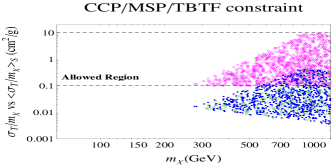
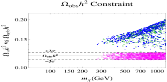
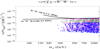
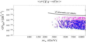
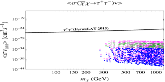
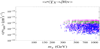
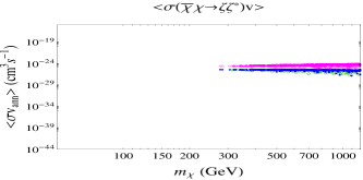
Figure 10: Predictions on $\sigma_{T}/m_{\chi}$, $\Omega h^{2}$, $\sigma^{SI}$, and $\langle\sigma_{\rm ann}v\rangle$ in different channels for all allowed samples. “${\color[rgb]{0,1,0}\circ}$” and “${\color[rgb]{0,0,1}\bullet}$” denote the samples which are testable for near future and below the neutrino floor, respectively, by the direct-detection experiment and without consideration of Sommerfeld effect. “${\color[rgb]{1,0,1}\diamond}$” denotes the values with considering the Sommerfeld effect

VII Model Parameter Space

In the CP-conserving LSDM model, there are eight free real parameters:

$$m_{\chi},m_{\zeta},\mu_{12},\lambda_{1},\lambda_{2},\lambda_{01},\lambda_{02},\,{\rm and}\,\lambda_{12}\,.$$

In this section, we look for favored regions of the parameter space in the LSDM model with implications from astrophysical and cosmological observations. We apply selection requirements for small scale structure, cold dark matter relic density, direct searches, and indirect detections, as well as cosmological constraints on right handed neutrinos.

For the leptonic scalar DM, the solution of small scale problem comes from DM strong self-interaction with $\sigma_{T}/m_{\chi}$ that contains 4 free parameters: $m_{\chi},m_{\zeta},\mu_{12}$ and $\lambda_{01}$, as shown in Eq. (71). At first, we perform a grid scan for the ranges, $m_{H}/2<m_{\chi}<1200\,\mathrm{GeV}$, $0.2<m_{\zeta}/\,\mathrm{GeV}<1$, and $-6<\log_{10}[\lambda_{01}]<\log_{10}[\sqrt{4\pi}]$. With these collected samples, we can pin down the corresponding allowed range for $\mu_{12}$ by using the allowed range of $\sigma_{T}/m_{\chi}$. Second, we use the interpolation technique to find the allowed range of $\mu_{12}$ from random sampling for $m_{\chi},m_{\zeta}$ and $\lambda_{12}$. We then apply random sampling with the 8 free parameters as usual except that $\mu_{12}$ is chosen from the allowed region with randomly selected $m_{\chi},m_{\zeta}$ and $\lambda_{12}$. Third, we use the selected parameters to find the allowed samples which satisfy the observed relic density constraint. Finally, we find the allowed parameter space by satisfying the constraints from the direct and indirect searches.

Following this procedure, we collect a thousand samples that satisfy all the constraints mentioned above. Fig. 10 shows the predictions in the LSDM model for $\sigma_{T}/m_{\chi}$, $\Omega_{\chi}h^{2}$, $\sigma^{SI}$, and $\langle\sigma_{\rm ann}v\rangle$ in $W^{+}W^{-},t\bar{t},\tau^{+}\tau^{-},\zeta H$ and $\zeta\zeta^{*}$ channels. Comparing the scenarios with and without Sommerfeld effect, we only depict those samples in agreement with XENON1T data in Fig. 10. The Sommerfeld effect is applied in the computation for the magenta samples “${\color[rgb]{1,0,1}\diamond}$”, while Green “${\color[rgb]{0,1,0}\circ}$” (testable for near future) and blue “${\color[rgb]{0,0,1}\bullet}$” (below the neutrino floor) are obtained without including the Sommerfeld effect. It is clear to see in Fig. 10(a), that the $\langle\sigma_{T}/m_{\chi}\rangle_{S}$ is enhanced by the Sommerfeld effect such that all values fall into $0.1\rm{\ (cm^{2}/g)}\leq\langle\sigma_{T}/m_{\chi}\rangle_{S}\leq 10\rm{\ (cm^{2}/g)}$. In Fig. 10(b), we see that the relic density is roughly proportional to $1/\langle\sigma_{\rm ann}\rangle$, and hence the $\Omega_{\chi}h^{2}$ becomes suppressed by the Sommerfeld effect such that the relic density of all selected samples fall into the range of $\Omega_{\rm obs}h^{2}\pm 3\sigma$.

It is interesting that the selected 1000 samples satisfying the small scale requirement (CCP/MSP/TBTF) and the observed relic density constraints also satisfy the the constraint on the SI DM-nucleon scattering cross section $\sigma^{SI}_{\chi p}$ shown in Fig. 10(c). We have extended XENON1T 2018 data to $m_{\chi}\simeq 1.2$ TeV with the dashed line. The cross section $\langle\sigma_{\rm ann}v\rangle$ for DM annihilating into $W^{+}W^{-}$, $t\bar{t}$, $\tau^{+}\tau^{-}$, $\zeta H$ and $\zeta\zeta^{*}$ channels are presented in Fig. 10(d)–Fig. 10(h). Combining indirect search in Fig. (8) and the small scale requirement, we see that the values of $\langle\sigma_{\rm ann}v\rangle$ can not be too large, and that $\chi\chi\to b\bar{b}$ and $\tau^{+}\tau^{-}$ may not be detectable.

Recall that the dominant $t$-channel cross section for the self-interacting leptonic scalar DM at the tree level is

$$\sigma(\chi\chi^{*}\to\chi\chi^{*})=\frac{\mu_{12}^{4}}{4\pi m_{\zeta}^{4}m_{\chi}^{2}}=\frac{g_{\zeta}^{2}\mu_{12}^{2}}{4\pi m_{\zeta}^{4}}\,.$$ (72)

The dimensionless coupling $g_{\zeta}\equiv\mu_{12}/m_{\chi}$ is important to determine the annihilation cross section, and it appears in the Yukawa potential [Eq. (48)] contributing to the Sommerfeld enhancement effects.

The value of $g_{\zeta}$ is modified by Sommerfeld enhancement with higher order and non-perturbative effects. Fig. 11 presents $g_{\zeta}$ as a function of $m_{\chi}$ with several values of $m_{\zeta}=$ 0.2 GeV (red “${\color[rgb]{1,0,0}\bullet}$”), 0.4 GeV (blue “${\color[rgb]{0,0,1}\times}$”), 0.6 GeV (blue “${\color[rgb]{0,0,1}\circ}$”), and 0.8 GeV (black “${\color[rgb]{0,0,0}\blacklozenge}$”). In addition, we consider four sets of parameters from top to bottom: $(\lambda_{01},\lambda_{02},\lambda_{12},f_{RR})$= $(10^{-6},10^{-6},10^{-6},10^{-6})$, $(0.1,10^{-3},0.1,0.0)$, $(0.2,10^{-3},0.2,0.2)$ and $(0.2,10^{-3},0.2,0.6)$, respectively. All allowed samples consistent with all mentioned constraints are denoted by green “${\color[rgb]{0,1,0}\diamond}$”. We find that $g_{\zeta}$ becomes larger with increasing value in $m_{\zeta}$ or decreasing values in the parameter set $(\lambda_{01},\lambda_{02},\lambda_{12},f_{RR})$. Note that for a given set of parameters, $\mu_{12}$ is randomly sampled to satisfy all mentioned constraint. The allowed range of $m_{\zeta}$ also depends on $m_{\chi}$.

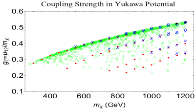
Figure 11: The dimensionless coupling strength $g_{\zeta}\equiv\mu_{12}/m_{\chi}$ in the Yukawa potential versus DM mass $m_{\chi}$ parametrized by the light mediator mass $m_{\zeta}$ where $m_{\zeta}=$ 0.2 GeV (red “${\color[rgb]{1,0,0}\bullet}$”), 0.4 GeV (blue “${\color[rgb]{0,0,1}\times}$”), 0.6 GeV (blue “${\color[rgb]{0,0,1}\circ}$”), and 0.8 GeV (black “${\color[rgb]{0,0,0}\blacklozenge}$”).

From the 1000 allowed samples that are consistent with all mentioned constraints, we can find the favored parameter space from the scanned region. BBN and CMB constraints require that $m_{\zeta}$ should be greater than 200 MeV, that leads to the minimal value of $m_{\chi}=276$ GeV. The maximal value of $m_{\zeta}$ is found to be 814 MeV corresponding to $m_{\chi}=1176$ GeV. $\lambda_{1}$ only involves the self-interaction process of $\chi\chi*\to\chi\chi^{*}$ in Eq. (71) and its contribution can be ignored even with $\lambda_{1}=\sqrt{4\pi}$. On the other hand, $\lambda_{2}$ is irrelevant in our calculation. We find that the maximal values of $\lambda_{01}$, $\lambda_{02}$, $\lambda_{12}$ and $f_{RR}$ are 0.27, 0.01 0.51 and 1.30, respectively. The allowed range of $\mu_{12}$ is between 75 and 634 GeV.

VIII Conclusions

We have adopted a special model that has a leptonic scalar dark matter (LSDM) ($\chi$) with lepton number $L_{\chi}=1$ and a light scalar mediator ($\zeta$) with $L_{\zeta}=2$ and three flavors of neutrino $\nu_{R}$ under the assumption of lepton number conservation. In the early Universe, DM thermalizes with SM particles via $H$-portal and $\chi\chi^{*}\to\zeta\zeta^{*}$ provides an efficient annihilation channel. After DM freezes out, all $\zeta$ decay into $\nu_{R}\nu_{R}$ with a lifetime $\tau_{\zeta}\lesssim 10^{-11}$ (sec) before the onset of BBN, and $\nu_{R}$ decouples from the SM particles at the temperature $T_{f}^{R}\sim m_{\zeta}$. The LSDM ($\chi$) and the light mediator ($\zeta$) with lepton number conservation can provide a self-interacting WIMP dark matter that is consistent with astrophysical and cosmological constraints.

In the LSDM model, the $t-$channel exchange of a light mediator ($\zeta$) makes the LSDM ($\chi$) self interacting cross section (SICS) reasonable large. Furthermore, we evaluate the the Sommerfeld effects and find significant enhancement for the SICS. That makes the LSDM model suitable to explain the small scale structure of the Universe.

We apply selection requirements for small scale structure, cold dark matter relic density (Planck), direct searches (XENON1T), and indirect detections (Fermi-LAT and H.E.S.S), as well as cosmological constraints on right-handed neutrinos. A randomly selected set of parameters was found with 1000 samples that satisfy all constraints. Large regions of the parameter space in the LSDM model are found to be consistent with astrophysical and cosmological observations and collider Higgs properties. A summary is in the following for the favored ranges of parameters:

• 0.2 GeV $\lesssim m_{\zeta}\lesssim$ 0.814 GeV (BBN, CMB),

• 276 GeV $\lesssim m_{\chi}\lesssim$ 1176 GeV (implied by $m_{\zeta}$),

• 75 GeV $\leq\mu_{12}\leq$ 634 GeV, and

• $\lambda_{02}\leq 10^{-2}$ (Higgs invisible width).

In addition, the upper bound of $\lambda_{01}$, $\lambda_{02}$ and $\lambda_{12}$ are 0.27, 0.01 and 0.51, respectively.

It is interesting that almost all regions of parameter space satisfying astrophysical and cosmological observations lead to a cold dark matter relic density with the most restrictive requirement Aghanim:2018eyx .

$$\Omega_{\rm c}h^{2}\pm 3\sigma=0.120\pm 0.001$$ (73)

that is

$$0.117\lesssim\Omega_{\chi}h^{2}\lesssim 0.123.$$ (74)

A more realistic requirement should be

$$\Omega_{\chi}h^{2}\lesssim 0.123\,.$$ (75)

That will enlarge the favored parameter space and accommodate more types of dark matter particles.

Appendix A Sommerfeld enhancement in $\chi\chi$ annihilations

A.1 Bethe-Salpeter equation in $\chi\chi\to\chi\chi$ process

The Feynman diagram of non-perturbative scattering $\chi(p_{1})\chi(p_{2})\to\chi(p_{3}^{\prime})\chi(p_{4}^{\prime})$ is shown in Fig. 5(a). Note that $p^{\prime}_{3}$ and $p^{\prime}_{4}$ are not necessary on-shell as these two lines will be connected to $\chi\chi$ annihilation diagrams later [see Fig. 5(b)]. Following the standard procedure Landau ; ChuaWong2017 , we will derive the Bathe-Salpeter equation for the process of scalar DM scattering via the scalar $H$-exchange repeatedly.

The amputated non-perturbative 4-point vertex function can be written as

$$i\Gamma(p^{\prime}_{3},p^{\prime}_{4};p_{1},p_{2}) = i\tilde{\Gamma}(p^{\prime}_{3},p^{\prime}_{4};p_{1},p_{2})$$ (76)

$$+\int\frac{d^{4}p^{\prime\prime}_{3}}{(2\pi)^{4}}i\tilde{\Gamma}(p^{\prime}_{3},p^{\prime}_{4};p^{\prime\prime}_{3},p^{\prime\prime}_{4})(iD_{F}(p^{\prime\prime}_{3}))i\Gamma(p^{\prime\prime}_{3},p^{\prime\prime}_{4};p_{1},p_{2})(iD_{F}(p^{\prime\prime}_{4})),$$

where we have $p^{\prime\prime}_{4}=p^{\prime}_{3}+p^{\prime}_{4}-p^{\prime\prime}_{3}$, $D_{F}$ is the scalar DM propagator and, the amputated tree-level 4-point vertex function through the $H$-exchange is given by

$$i\tilde{\Gamma}(p^{\prime}_{3},p^{\prime}_{4};p^{\prime\prime}_{3},p^{\prime\prime}_{4})=-i\lambda_{01}^{2}v^{2}\frac{1}{(p^{\prime\prime}_{3}-p^{\prime}_{3})^{2}-m^{2}_{H}}.$$ (77)

With the instantaneous approximation, namely, ignoring the time component of the momentum transfer, the tree-level 4-point vertex function is just the potential $U_{H}(\vec{p}\ ^{\prime\prime}_{3}-\vec{p}\ ^{\prime}_{3})$ defined below

$$i\tilde{\Gamma}(p^{\prime}_{3},p^{\prime}_{4};p^{\prime\prime}_{3},p^{\prime\prime}_{4})=i\lambda_{01}^{2}v^{2}\frac{1}{(\vec{p}\ ^{\prime\prime}_{3}-\vec{p}\ ^{\prime}_{3})^{2}+m^{2}_{H}}\equiv iU_{H}(\vec{p}\ ^{\prime\prime}_{3}-\vec{p}\ ^{\prime}_{3}).$$ (78)

To proceed we define two auxiliary functions as follows ChuaWong2017 :

$$i\eta(p_{3},p_{4};p_{1},p_{2}) \equiv iD_{F}(p_{3})i\Gamma(p_{3},p_{4};p_{1},p_{2})(iD_{F}(p_{4})),$$

$$i\tilde{\chi}(p_{3},p_{4};p_{1},p_{2}) \equiv iD_{F}(p_{3})i\tilde{\Gamma}(p_{3},p_{4};p_{1},p_{1})(iD_{F}(p_{4})),$$ (79)

and Eq. (76) can be expressed as

$$i\eta(p^{\prime}_{3},p^{\prime}_{4};p_{1},p_{2}) = i\tilde{\chi}(p^{\prime}_{3},p^{\prime}_{4};p_{1},p_{2})$$ (80)

$$+\int\frac{d^{4}p^{\prime\prime}_{3}}{(2\pi)^{4}}i\tilde{\chi}(p^{\prime}_{3},p^{\prime}_{4};p^{\prime\prime}_{3},p^{\prime\prime}_{4})i\eta(p^{\prime\prime}_{3},p^{\prime\prime}_{4};p_{1},p_{2}).$$

Adding $(2\pi)^{4}\delta^{4}(p^{\prime\prime}_{3}-p_{1})$ to both side of the above equation, and defining

$$i\chi(p^{\prime}_{3},p^{\prime}_{4};p_{1},p_{2}) \equiv (2\pi)^{4}\delta^{4}(p^{\prime\prime}_{3}-p^{\prime}_{3})+i\eta(p^{\prime}_{3},p^{\prime}_{4};p_{1},p_{2}),$$ (81)

Eq. (80) becomes

$$i\chi(p^{\prime}_{3},p^{\prime}_{4};p_{1},p_{2})=(2\pi)^{4}\delta^{4}(p^{\prime\prime}_{3}-p^{\prime}_{3})+\int\frac{d^{4}p^{\prime\prime}_{3}}{(2\pi)^{4}}i\tilde{\chi}(p^{\prime}_{3},p^{\prime}_{4};p^{\prime\prime}_{3},p^{\prime\prime}_{4})i\chi(p^{\prime\prime}_{3},p^{\prime\prime}_{4};p_{1},p_{2}).$$ (82)

In the NR limit, the scalar propagator can be approximately written as

$$D_{F}(\pm k)=\frac{1}{2m_{\chi}}\frac{1}{(k_{0}-m_{\chi})-\vec{k}^{2}/2m_{\chi}+i\epsilon}\equiv\frac{1}{2m_{\chi}}g_{\chi}(k),$$ (83)

Substitute it into the above equation, we obtain the equation for $\chi$,

$$i\chi(p^{\prime}_{3},p^{\prime}_{4};p_{1},p_{2})=(2\pi)^{4}\delta^{4}(p^{\prime\prime}_{3}-p^{\prime}_{3})+\frac{1}{4m_{\chi}^{2}}g_{\chi}(p^{\prime}_{3})g_{\chi}(p^{\prime}_{4})\int\frac{d^{4}p^{\prime\prime}_{3}}{(2\pi)^{4}}U_{H}(\vec{p}^{\prime\prime}_{3}-\vec{p}^{\prime}_{3})\chi(p^{\prime\prime}_{3},p^{\prime\prime}_{4};p_{1},p_{2}).$$

(84)

In fact, we can drop the redundant variables $p_{1}$ and $p_{2}$ in the above equation. Now we define

$$\left\{\begin{array}[]{rcl}&&p\equiv(p^{\prime}_{3}-p^{\prime}_{4})/2\\ &&P\equiv(p^{\prime}_{3}+p^{\prime}_{4})/2\\ &&\hat{\chi}(k_{1},k_{2})\equiv\chi(k_{1}+k_{2},k_{1}-k_{2})\\ \end{array}\right..$$ (88)

Eq. (84) can be rewritten as

$$i\hat{\chi}(P,p)=(2\pi)^{4}\delta^{4}(q-P-p)+\frac{1}{4m_{\chi}^{2}}g_{\chi}(P+p)g_{\chi}(P-p)\int\frac{d^{4}q}{(2\pi)^{4}}U_{H}(\vec{q}-\vec{P}-\vec{p})\hat{\chi}(P,q-P).$$

Let $q^{\prime}=q-P$ and redefine $q^{\prime}=q$. The above equation becomes

$$i\hat{\chi}(P,p)=(2\pi^{4})\delta^{4}(q-p)+\frac{1}{4m_{\chi}^{2}}g_{\chi}(P+p)g_{\chi}(P-p)\int\frac{d^{4}q}{(2\pi)^{4}}U_{H}(\vec{q}-\vec{p})\hat{\chi}(P,q).$$ (90)

Defining the Bathe-Salpeter wave function as

$$\psi(\vec{q})\equiv\int\frac{dq_{0}}{2\pi}i\hat{\chi}(P,q),$$ (91)

and integrating with respect to $p_{0}$ on both sides of Eq. (90), we have

$$\psi(\vec{p})=(2\pi)^{3}\delta(\vec{q}-\vec{p})+\frac{1}{2\pi i}\frac{1}{4m_{\chi}^{2}}\int dp_{0}\ g_{\chi}(P+p)g_{\chi}(P-p)\int\frac{d^{3}\vec{q}}{(2\pi)^{3}}U_{H}(\vec{q}-\vec{p})\psi(\vec{q}).$$

(92)

By taking $p^{\prime}_{3}=(E^{\prime}_{3},\vec{p})$, $p^{\prime}_{4}=(E^{\prime}_{4},-\vec{p})$, $p^{\prime\prime}_{3}=(E^{\prime\prime}_{3},\vec{p})$ and $p^{\prime}_{4}=(E^{\prime\prime}_{4},-\vec{p})$ in the center of mass frame, we have $p\equiv(\epsilon,\vec{p})=((E^{\prime}_{3}-E^{\prime}_{4})/2,\vec{p})$ and $P\simeq(m_{\chi}+E/2,\vec{0})$ and the total kinetic energy $E=\mu v^{2}/2$ where $\mu=m_{\chi}/2$ is the reduce mass of $\chi\chi$ system and the relative velocity $v=v_{\rm lab}$ defined in Eq. 30. Using the residue theorem, we integrate over $p_{0}=\epsilon$ in Eq.(92), and obtain

$$\psi(\vec{p})=(2\pi)^{3}\delta(\vec{q}-\vec{p})+\frac{1}{E-\frac{\vec{p}^{2}}{m_{\chi}}}\int\frac{d^{3}\vec{q}}{(2\pi)^{3}}V_{H}(\vec{q}-\vec{p})\psi(\vec{q}),\quad V_{H}(\vec{q})\equiv-\frac{1}{4m_{\chi}^{2}}U_{H}(\vec{q}),$$ (93)

The above equation is simply the Bathe-Salpeter equation in the momentum space representation. By taking the Fourier transformation, we have

$$\int\frac{d^{3}\vec{p}}{(2\pi)^{3}}e^{-i\vec{p}\cdot\vec{r}}(\frac{\vec{p}^{2}}{m_{\chi}}-E)[\psi(\vec{p})+(2\pi)^{3}\delta(\vec{q}-\vec{p})]+\int\frac{d^{3}\vec{p}}{(2\pi)^{3}}e^{-i\vec{p}\cdot\vec{r}}\int\frac{d^{3}\vec{q}}{(2\pi)^{3}}V_{H}(\vec{q}-\vec{p})\psi(\vec{q})=0.$$

After simplification, we obtain the Bathe-Salpeter equation in the position representation:

$$-\frac{1}{2\mu}\nabla^{2}\psi(\vec{r})+V_{H}(r)\psi(\vec{r})=E\psi(\vec{r}),\quad V_{H}(r)=-\alpha_{H}\frac{e^{-m_{H}r}}{r},$$ (95)

where we see the potential is Yukawa-type with the corresponding fine structure constant $\alpha_{H}=g_{H}^{2}/4\pi$ and the dimensionless coupling strength $g_{H}=\lambda_{01}v/2m_{\chi}$.

A.2 s-wave Sommerfeld factor in $\chi\chi\to\nu_{R}\nu_{R}$ process

From Fig. 5(b), the Sommerfeld enhanced amplitude $iA_{S}$ of $\chi\chi\to\nu_{R}\nu_{R}$ annihilation process can be expressed as

$$iA_{S}(p_{3},p_{4},p_{1},p_{2}) = iA(p_{3},p_{4},p_{1},p_{2})$$ (96)

$$+ \int\frac{d^{4}p^{\prime}_{3}}{(2\pi)^{4}}iA(p_{3},p_{4};p^{\prime}_{3},p^{\prime}_{4})(iD_{F}(p^{\prime}_{3}))i\Gamma(p^{\prime}_{3},p^{\prime}_{4};p_{1},p_{2})(iD_{F}(p^{\prime}_{4}))$$

where $iA$ is the amplitude of the process at tree level. With the help of Eq. (79), we have

$$iA_{S}(p_{3},p_{4};p_{1},p_{2})=\int\frac{d^{4}p^{\prime}_{3}}{(2\pi)^{4}}iA(p_{3},p_{4};p^{\prime}_{3},p^{\prime}_{4})i\chi(p^{\prime}_{3},p^{\prime}_{4};p_{1},p_{2}).$$ (97)

For the s-wave rescattering, the amplitude $A(p_{3},p_{4};p^{\prime}_{3},p^{\prime}_{4})$ is independent of momentum and hence, the above equation becomes

$$iA_{S}(p_{3},p_{4},;p_{1},p_{2}) = iA(p_{3},p_{4};p_{1},p_{2})\int\frac{d^{3}\vec{p}}{(2\pi)^{4}}\int\frac{dp_{0}}{(2\pi)}i\hat{\chi}(P,p)$$ (98)

$$= iA(p_{3},p_{4};p_{1},p_{2})\psi_{l=0}(\vec{r}=0)$$

Hence we have

$$|A_{S}(p_{3},p_{4},;p_{1},p_{2})|^{2}=|A_{(}p_{3},p_{4},;p_{1},p_{2})|^{2}S,$$ (99)

where $S=|\psi_{l=0}(\vec{r}=0)|^{2}$ is the so-called s-wave Sommerfeld factor and the wave function $\psi(\vec{r})$ satisfies the Bathe-Salpeter Equation in Eq. (95).

A.3 Solving $\psi(\vec{r}=0)$ numerically

Let us consider the general case. As we know that two DM particles form a bound $\chi\chi$ or $\chi\chi^{*}$ state before annihilation. This two-particle wave function $\psi(\vec{r})$ satisfies the following Schrödinger equation [see in Eq. (47) ]

$$-\frac{1}{2\mu}\nabla^{2}\psi(\vec{r})+V(\vec{r})\psi(\vec{r})=E\psi(\vec{r})=\frac{1}{2}\mu v^{2}\psi(\vec{r}).$$ (100)

The separation of variables give us the radial Schrödinger equation

$$[-\frac{1}{2\mu}\frac{1}{r^{2}}\frac{d}{dr}(r^{2}\frac{d}{dr})+V(r)+\frac{l(l+1)}{2\mu r^{2}}]R_{l}(r)=ER_{l}(r).$$ (101)

Here we follow Iengo:2009ni ; ChuaWong2017 to solve for $\psi(\vec{r}=0)$ numerically. From the scattering theory, the radial wave function has the following asymptotic form Sakurai :

$$R_{l}(r)\rightarrow e^{i\delta_{l}}\frac{\sin(pr-l\pi/2+\delta_{l})}{pr},$$ (102)

where $\delta_{l}$ is the phase shift corresponding to the partial wave with angular momentum quantum number $l$. Defining $\Phi_{l}$ by $R_{l}(\rho)=N\rho^{l}\Phi_{l}(r)$ with $\rho=pr$, and normalization constant $N$ to be determined later, Eq. (101) becomes

$$\Phi^{\prime\prime}_{l}+\frac{2(l+1)}{\rho}\Phi^{\prime}_{l}+(-\frac{2}{pv}V(r)+1)\Phi_{l}=0,$$ (103)

where the initial conditions are taken to be Iengo:2009ni

$$\Phi_{l}(0)=1,\quad\Phi^{\prime}_{l}(0)=\frac{\rho V(r)}{pv(l+1)}\bigg{|}_{\rho\to{0}}\Phi_{l}(0),$$ (104)

for a regular solution. We now concentrate on the $l=0$ case. As one can see by taking $\rho\gg 1$, in the case that $|\rho V(r)|\ll 1$, the differential equation and its solution become

$$\Phi^{\prime\prime}_{0}+\frac{2}{\rho}\Phi^{\prime}_{0}+\Phi_{0}\bigg{|}_{\rho\gg 1}=0,\qquad\Phi_{0}(\rho)\to C\frac{\sin(\rho+\delta_{0})}{\rho},$$ (105)

with $C$ a real number. The above $\Phi_{0}$ is to be compared to $R_{0}(r)\to e^{i\delta_{0}}\sin(\rho+\delta_{0})/\rho$ [see Eq. (102)], as $\rho\gg 1$. To work out the normalization $N$, it is useful noting, in the $\rho\gg 1$ region,

$$\Phi_{0}(\rho-\pi/2)\to-C\frac{\cos(\rho+\delta_{0})}{\rho-\pi/2},$$ (106)

which can be used with $\Phi_{0}(\rho)$ to construct

$$\kappa\equiv\lim_{\rho\to\infty}e^{i\rho}\left[{-i\rho\Phi_{0}(\rho)-(\rho-\pi/2)\Phi_{0}(\rho-\pi/2)}\right]=Ce^{-i\delta_{0}}.$$ (107)

Consequently, we see that $R_{0}(r)$ can be obtained as

$$R_{0}(r)=\kappa^{-1}\Phi_{0}(\rho),$$ (108)

since it satisfies the Schrödinger equation and has the correct asymptotic behavior. Finally, we have

$$\psi(\vec{r}=0)=\kappa^{-1}\Phi_{0}(0)=\kappa^{-1}=\lim_{\rho\to\infty}\frac{e^{-i\rho}}{-i\rho\Phi_{0}(\rho)-(\rho-\pi/2)\Phi_{0}(\rho-\pi/2)}.$$ (109)

Note that the phase of $\psi(\vec{r}=0)$ is just $\delta_{0}$ [see Eq. (107)].

Now we are ready to do the numerical calculation. For a scalar DM $\chi$ with a scalar mediator $X$, we have the Yukawa-type potential:

$$V_{X}(r)=-\alpha_{X}\frac{e^{-m_{X}r}}{r},$$ (110)

where $\alpha_{X}=g_{X}^{{}^{\prime}2}/(16\pi m_{\chi}^{2})$ with the dimensionful coupling strength $g^{\prime}_{X}=\lambda_{01}{\rm v}$, namely, the dimensionless coupling strength $g_{X}=g^{\prime}_{X}/2m_{\chi}$. Hence we need to solve the following differential equation:

$$\Phi^{\prime\prime}(\rho)+\frac{2}{x}\Phi^{\prime}(\rho)+(1-\frac{2a_{X}e^{-b_{X}\rho}}{\rho})\Phi(\rho)=0,$$ (111)

with the boundary conditions:

$$\Phi(\rho=0)=1,\quad\Phi^{\prime}(\rho=0)=-a_{X}.$$ (112)

In the above $a_{X}=\alpha_{X}$ and $b_{X}=2m_{X}/m_{\chi}v$. We find that it is enough to take $\rho\simeq 200$ to obtain the limit in Eq. (109).

References

- (1) F. Zwicky, Helv. Phys. Acta 6, 110 (1933).
- (2) V. C. Rubin and W. K. Ford, Jr., “Rotation of the Andromeda Nebula from a Spectroscopic Survey of Emission Regions,” Astrophys. J. 159, 379 (1970).
- (3) K. G. Begeman, A. H. Broeils and R. H. Sanders, “Extended rotation curves of spiral galaxies: Dark haloes and modified dynamics,” Mon. Not. Roy. Astron. Soc. 249, 523 (1991).
- (4) S. M. Carroll, “Dark matter is real,” Nature Phys. 21, 653 (2006).
- (5) D. Clowe, M. Bradac, A. H. Gonzalez, M. Markevitch, S. W. Randall, C. Jones and D. Zaritsky, “A direct empirical proof of the existence of dark matter,” Astrophys. J. 648, L109 (2006) [astro-ph/0608407].
- (6) D. N. Spergel et al. [WMAP Collaboration], “First year Wilkinson Microwave Anisotropy Probe (WMAP) observations: Determination of cosmological parameters,” Astrophys. J. Suppl. 148, 175 (2003) [astro-ph/0302209].
- (7) M. Tegmark et al. [SDSS Collaboration], “Cosmological parameters from SDSS and WMAP,” Phys. Rev. D 69, 103501 (2004) [astro-ph/0310723].
- (8) N. Aghanim et al. [Planck], Astron. Astrophys. 641 (2020), A6 doi:10.1051/0004-6361/201833910 [arXiv:1807.06209 [astro-ph.CO]].
- (9) M. Colless et al. [2DFGRS Collaboration], Mon. Not. Roy. Astron. Soc. 328, 1039 (2001) [astro-ph/0106498].
- (10) V. Springel, C. S. Frenk and S. D. M. White, Nature 440, 1137 (2006) [astro-ph/0604561].
- (11) B. Moore, Nature 370, 629 (1994).
- (12) P. Salucci, Astron. Astrophys. Rev. 27, no.1, 2 (2019) [arXiv:1811.08843 [astro-ph.GA]].
- (13) B. Moore, S. Ghigna, F. Governato, G. Lake, T. R. Quinn, J. Stadel and P. Tozzi, Astrophys. J. 524, L19 (1999) [astro-ph/9907411].
- (14) M. Boylan-Kolchin, J. S. Bullock and M. Kaplinghat, Mon. Not. Roy. Astron. Soc. 415, L40 (2011) [arXiv:1103.0007 [astro-ph.CO]].
- (15) M. Boylan-Kolchin, J. S. Bullock and M. Kaplinghat, Mon. Not. Roy. Astron. Soc. 422, 1203-1218 (2012) [arXiv:1111.2048 [astro-ph.CO]].
- (16) D. N. Spergel and P. J. Steinhardt, Phys. Rev. Lett. 84, 3760 (2000) [astro-ph/9909386].
- (17) M. Rocha, A. H. G. Peter, J. S. Bullock, M. Kaplinghat, S. Garrison-Kimmel, J. Onorbe and L. A. Moustakas, Mon. Not. Roy. Astron. Soc. 430, 81 (2013) [arXiv:1208.3025 [astro-ph.CO]].
- (18) O. D. Elbert, J. S. Bullock, S. Garrison-Kimmel, M. Rocha, J. Oñorbe and A. H. G. Peter, Mon. Not. Roy. Astron. Soc. 453, no. 1, 29 (2015) doi:10.1093/mnras/stv1470 [arXiv:1412.1477 [astro-ph.GA]].
- (19) O. Adriani et al. [PAMELA Collaboration], Nature 458, 607 (2009) [arXiv:0810.4995 [astro-ph]].
- (20) O. Adriani et al. [PAMELA Collaboration], Phys. Rev. Lett. 111, 081102 (2013) [arXiv:1308.0133 [astro-ph.HE]].
- (21) J. Chang et al., Nature 456, 362 (2008).
- (22) A. A. Abdoet al. [Fermi LAT Collaboration], Phys. Rev. Lett. 102, 181101 (2009).
- (23) J. L. Feng, M. Kaplinghat and H. B. Yu, Phys. Rev. Lett. 104, 151301 (2010) [arXiv:0911.0422 [hep-ph]].
- (24) M. Kaplinghat, T. Linden and H. B. Yu, Phys. Rev. Lett. 114, no. 21, 211303 (2015) [arXiv:1501.03507 [hep-ph]].
- (25) E. Ma, Mod. Phys. Lett. A 33, no. 38, 1850226 (2018) [arXiv:1805.03295 [hep-ph]].
- (26) T. Bringmann, F. Kahlhoefer, K. Schmidt-Hoberg and P. Walia, Phys. Rev. Lett. 118, no. 14, 141802 (2017) [arXiv:1612.00845 [hep-ph]].
- (27) E. Aprile et al. [XENON Collaboration], Phys. Rev. Lett. 121, no. 11, 111302 (2018) [arXiv:1805.12562 [astro-ph.CO]].
- (28) M. Tanabashi et al. [Particle Data Group], Phys. Rev. D 98, no.3, 030001 (2018)
- (29) M. Ackermann et al. [Fermi-LAT Collaboration], “Searching for Dark Matter Annihilation from Milky Way Dwarf Spheroidal Galaxies with Six Years of Fermi Large Area Telescope Data,” Phys. Rev. Lett. 115, no. 23, 231301 (2015) [arXiv:1503.02641 [astro-ph.HE]].
- (30) A. Albert et al. [Fermi-LAT and DES Collaborations], Astrophys. J. 834, no. 2, 110 (2017) [arXiv:1611.03184 [astro-ph.HE]].
- (31) H. Abdallah et al. [H.E.S.S. Collaboration], “Search for dark matter annihilations towards the inner Galactic halo from 10 years of observations with H.E.S.S,” Phys. Rev. Lett. 117, no. 11, 111301 (2016) [arXiv:1607.08142 [astro-ph.HE]].
- (32) C. Bonilla, E. Ma, E. Peinado and J. W. F. Valle, Phys. Lett. B 762, 214 (2016) [arXiv:1607.03931 [hep-ph]].
- (33) E. Ma and O. Popov, Phys. Lett. B 764, 142 (2017) [arXiv:1609.02538 [hep-ph]].
- (34) E. Ma and U. Sarkar, Phys. Lett. B 776, 54 (2018) [arXiv:1707.07698 [hep-ph]].
- (35) E. Aprile et al. [XENON], [arXiv:2006.09721 [hep-ex]].
- (36) T. P. Cheng, “Chiral Symmetry and the Higgs Nucleon Coupling,” Phys. Rev. D 38, 2869 (1988).
- (37) H. Y. Cheng, “Low-energy Interactions of Scalar and Pseudoscalar Higgs Bosons With Baryons,” Phys. Lett. B 219, 347 (1989).
- (38) J. Gasser, H. Leutwyler and M. E. Sainio, “Sigma term update,” Phys. Lett. B 253, 252 (1991).
- (39) J. M. Alarcon, J. Martin Camalich and J. A. Oller, Phys. Rev. D 85, 051503 (2012) [arXiv:1110.3797 [hep-ph]].
- (40) J. M. Alarcon, L. S. Geng, J. Martin Camalich and J. A. Oller, Phys. Lett. B 730, 342 (2014) [arXiv:1209.2870 [hep-ph]].
- (41) H. Y. Cheng and C. W. Chiang, “Revisiting Scalar and Pseudoscalar Couplings with Nucleons,” JHEP 1207, 009 (2012) [arXiv:1202.1292 [hep-ph]].
- (42) M. A. Shifman, A. I. Vainshtein and V. I. Zakharov, “Remarks on Higgs Boson Interactions with Nucleons,” Phys. Lett. B 78, 443 (1978).
- (43) G. Jungman, M. Kamionkowski and K. Griest, “Supersymmetric dark matter,” Phys. Rept. 267, 195 (1996) [hep-ph/9506380].
- (44) J. Menendez, D. Gazit and A. Schwenk, “Spin-dependent WIMP scattering off nuclei,” Phys. Rev. D 86, 103511 (2012) [arXiv:1208.1094 [astro-ph.CO]].
- (45) C. K. Chua and G. G. Wong, “Study of Majorana Fermionic Dark Matter,” Phys. Rev. D 94, no. 3, 035002 (2016) [arXiv:1512.01991 [hep-ph]].
- (46) J. D. Lewin and P. F. Smith, “Review of mathematics, numerical factors, and corrections for dark matter experiments based on elastic nuclear recoil,” Astropart. Phys. 6, 87 (1996).
- (47) L. Vietze, P. Klos, J. Menendez, W. C. Haxton and A. Schwenk, “Nuclear structure aspects of spin-independent WIMP scattering off xenon,” Phys. Rev. D 91, no. 4, 043520 (2015) [arXiv:1412.6091 [nucl-th]].
- (48) J. Billard, L. Strigari and E. Figueroa-Feliciano, Phys. Rev. D 89, no. 2, 023524 (2014)
- (49) B. Cabrera, L. M. Krauss and F. Wilczek, Phys. Rev. Lett. 55, 25 (1985).
- (50) J. Monroe and P. Fisher, Phys. Rev. D 76, 033007 (2007)
- (51) E. W. Kolb and M. S. Turner, “The Early Universe,” Front. Phys. 69, 1 (1990).
- (52) T. S. Coleman and M. Roos, “Effective degrees of freedom during the radiation era,” Phys. Rev. D 68, 027702 (2003) [astro-ph/0304281].
- (53) L. Rinchiuso [H.E.S.S.], EPJ Web Conf. 209, 01023 (2019) doi:10.1051/epjconf/201920901023 [arXiv:1901.05299 [astro-ph.HE]].
- (54) A. Albert et al. [HAWC Collaboration], Astrophys. J. 853, no. 2, 154 (2018) [arXiv:1706.01277 [astro-ph.HE]].
- (55) M. L. Ahnen et al. [MAGIC Collaboration], JCAP 1803, 009 (2018) [arXiv:1712.03095 [astro-ph.HE]].
- (56) S. Archambault et al. [VERITAS Collaboration], Phys. Rev. D 95, no. 8, 082001 (2017) [arXiv:1703.04937 [astro-ph.HE]].
- (57) A. Albert et al. [ANTARES], data,” Phys. Lett. B 805, 135439 (2020) doi:10.1016/j.physletb.2020.135439 [arXiv:1912.05296 [astro-ph.HE]].
- (58) A. Albert et al. [ANTARES and IceCube], ctic Center with ANTARES and IceCube,” Phys. Rev. D 102, no.8, 082002 (2020) doi:10.1103/PhysRevD.102.082002 [arXiv:2003.06614 [astro-ph.HE]].
- (59) C. S. Kochanek, “The Mass of the Milky Way galaxy,” Astrophys. J. 457, 228 (1996) [astro-ph/9505068].
- (60) F. Ferrer and D. R. Hunter, JCAP 09, 005 (2013) doi:10.1088/1475-7516/2013/09/005 [arXiv:1306.6586 [astro-ph.HE]].
- (61) J. Hisano, S. Matsumoto and M. M. Nojiri, “Explosive dark matter annihilation,” Phys. Rev. Lett. 92, 031303 (2004) [hep-ph/0307216].
- (62) J. Hisano, S. Matsumoto, M. M. Nojiri and O. Saito, “Non-perturbative effect on dark matter annihilation and gamma ray signature from galactic center,” Phys. Rev. D 71, 063528 (2005) [hep-ph/0412403].
- (63) J. Hisano, S. Matsumoto, M. Nagai, O. Saito and M. Senami, “Non-perturbative effect on thermal relic abundance of dark matter,” Phys. Lett. B 646, 34 (2007) [hep-ph/0610249].
- (64) N. Arkani-Hamed, D. P. Finkbeiner, T. R. Slatyer and N. Weiner, “A Theory of Dark Matter,” Phys. Rev. D 79, 015014 (2009) [arXiv:0810.0713 [hep-ph]].
- (65) E. J. Chun, J. C. Park and S. Scopel, JCAP 1212, 022 (2012) [arXiv:1210.6104 [astro-ph.CO]].
- (66) E. J. Chun and J. C. Park, “Electro-Weak Dark Matter: non-perturbative effect confronting indirect detections,” Phys. Lett. B 750, 372 (2015) [arXiv:1506.07522 [hep-ph]].
- (67) E. J. Chun, S. Jung and J. C. Park, “Very Degenerate Higgsino Dark Matter,” JHEP 1701, 009 (2017) [arXiv:1607.04288 [hep-ph]].
- (68) S. Cassel, “Sommerfeld factor for arbitrary partial wave processes,” J. Phys. G 37, 105009 (2010) [arXiv:0903.5307 [hep-ph]].
- (69) C. K. Chua and G. G. Wong, Phys. Rev. D 96, no. 11, 115006 (2017) [arXiv:1708.08624 [hep-ph]].
- (70) J. L. Feng, M. Kaplinghat and H. -B. Yu, “Sommerfeld Enhancements for Thermal Relic Dark Matter,” Phys. Rev. D 82, 083525 (2010) [arXiv:1005.4678 [hep-ph]]; T. R. Slatyer, “The Sommerfeld enhancement for dark matter with an excited state,” JCAP 1002, 028 (2010) [arXiv:0910.5713 [hep-ph]].
- (71) L. D. Landau and E. M. Lifshitz, “Quantum Mechanics : Non-Relativistic Theory,” (Course of theoretical physics III, 3rd ed.), Pergamon Press (1977).
- (72) N. N. Lebedev, translated by R. Silverman, “Special Functions & Their Applications,” (Dover Books on Mathematics), Dover Publications, Revised ed. edition (1972), pp. 15, 261.
- (73) G. Mangano, G. Miele, S. Pastor, T. Pinto, O. Pisanti and P. D. Serpico, Nucl. Phys. B 729, 221 (2005) [hep-ph/0506164].
- (74) F. Iocco, G. Mangano, G. Miele, O. Pisanti and P. D. Serpico, Phys. Rept. 472, 1 (2009) [arXiv:0809.0631 [astro-ph]].
- (75) J. Zhang and S. Zhou, Nucl. Phys. B 903, 211 (2016) [arXiv:1509.02274 [hep-ph]].
- (76) E. M. Lifshitz and L. P. Pitaevskii, “Relativistic Quantum Theory,” ( Volume 4 part 1 of A Course of Theoretical Physics ), Pergamon Press (1973).
- (77) R. Iengo, “Sommerfeld enhancement: General results from field theory diagrams,” JHEP 0905, 024 (2009) [arXiv:0902.0688 [hep-ph]].
- (78) J. J. Sakurai and J. Napolitano, “Modern quantum physics,” Boston, USA: Addison-Wesley (2011).