Optimizing Deeper Transformers on Small Datasets

Abstract

It is a common belief that training deep transformers from scratch requires large datasets. Consequently, for small datasets, people usually use shallow and simple additional layers on top of pre-trained models during fine-tuning. This work shows that this does not always need to be the case: with proper initialization and optimization, the benefits of very deep transformers can carry over to challenging tasks with small datasets, including Text-to-SQL semantic parsing and logical reading comprehension. In particular, we successfully train $48$ layers of transformers, comprising $24$ fine-tuned layers from pre-trained RoBERTa and $24$ relation-aware layers trained from scratch. With fewer training steps and no task-specific pre-training, we obtain the state-of-the-art performance on the challenging cross-domain Text-to-SQL parsing benchmark Spider. We achieve this by deriving a novel Data-dependent Transformer Fixed-update initialization scheme (DT-Fixup), inspired by the prior T-Fixup work Huang et al. (2020). Further error analysis shows that increasing depth can help improve generalization on small datasets for hard cases that require reasoning and structural understanding.

1 Introduction

In recent years, large-scale pre-trained language models Radford et al. (2019); Devlin et al. (2018); Liu et al. (2019b) trained with transformers Vaswani et al. (2017) have become standard building blocks of modern NLP systems to help improve generalization when task-specific annotations are limited. In practice, it has been found that deeper transformers generally yield better results with sufficient training data Lan et al. (2019), especially on tasks involving reasoning and structural understanding. This suggests that additional transformer layers should be employed in conjunction with pre-trained models, instead of simple and shallow neural components, such as a classifier head, currently used by models of many NLP tasks. However, the common belief in the literature is that training deep transformers from scratch requires large datasets, and few attempts have been made on small datasets, to the best of our knowledge. One implication is that although extra transformer layers on top of pre-trained models should help with more challenging problems in principle, it does not work in practice due to limited training data. We show that after resolving several optimization issues with the method proposed in this work, it is possible to train very deep transformers with improved generalization even on small datasets.

One advantage of pre-trained models is the reduced computational resources needed when fine-tuning on small datasets. For instance, it allows practitioners to finetune on a single GPU and obtain strong performance on a downstream task. However, the large size of pre-trained models limits the batch size that can be used in training new transformer layers on a small computational budget. Despite their broad applications, training transformer models is known to be difficult (Popel and Bojar, 2018). The standard transformer training approach leverages learning rate warm-up, layer normalization Ba et al. (2016) and a large batch size, and models typically fail to learn when missing any one of these components. The restricted batch size aggravates the training difficulties. Even if a large batch size can be feasibly employed, poorer generalization results are often observed Keskar et al. (2016), especially when the dataset size is only several times larger than the batch size. Furthermore, many recent works noticed a performance gap in this training approach due to layer normalization Xu et al. (2019); Nguyen and Salazar (2019); Zhang et al. (2019a); Wang et al. (2019b); Liu et al. (2020); Huang et al. (2020).

Inspired by the recent T-Fixup by Huang et al. (2020), which eliminates the need for learning rate warm-up and layer normalization to train vanilla transformers, we derive a data-dependent initialization strategy by applying different analyses to address several key limitations of T-Fixup. We call our method the Data-dependent Transformer Fixed-update initialization scheme, DT-Fixup. In the mixed setup of additional yet-to-be-trained transformers on top of pre-trained models, DT-Fixup enables the training of significantly deeper transformers, and is generally applicable to different neural architectures. Our derivation also extends beyond vanilla transformers to transformers with relational encodings Shaw et al. (2018), allowing us to apply the results to one variant called relation-aware transformer Wang et al. (2019a). By applying DT-Fixup on different tasks, we show that the impression that deep transformers do not work on small datasets stems from the optimization procedure rather than the architecture. With proper initialization and optimization, training extra transformer layers is shown to facilitate the learning of complex relations and structures in the data.

We verify the effectiveness of DT-Fixup on Spider Yu et al. (2018), a complex and cross-domain Text-to-SQL semantic parsing benchmark, and ReColr Yu et al. (2020b), a reading comprehension dataset requiring logical reasoning. While Text-to-SQL semantic parsing is inherently different from reading comprehension, they share similar characteristics which require certain levels of reasoning and structural understanding ability. Meanwhile, the sizes of both datasets are less than 10k training samples, which is tiny by deep learning standards and renders large-batch training undesirable due to poor generalization.

On both datasets, DT-Fixup consistently outperforms the standard approach with better generalization and allows the training of significantly deeper transformer models. For Spider, we successfully apply DT-Fixup to train a Text-to-SQL parser containing $48$ transformer layers, with $24$ relation-aware layers trained from scratch on top of $24$ pre-trained layers from pre-trained RoBERTa Liu et al. (2019b). Our parser achieves $70.9\%$ exact match accuracy on the Spider test set, which is the state of the art at the time of writing. At the same time, it requires less training steps and no task-specific pre-training as compared to the prior art Yu et al. (2020a). For ReClor, we rank the second on the public leaderboard by simply adding $4$ transformer layers on top of RoBERTa. Further error analysis shows that the performance improvements by increasing the depth mainly come from better generalization on the harder cases requiring reasoning and structural understanding. Even the failed predictions from the deep models are more reasonable than from the shallow ones.

2 Background

In this section, we present the necessary background by first introducing the relation-aware transformer layer, which outperforms the vanilla transformer layer with limited data by injecting additional inductive bias Wang et al. (2019a). Then, we introduce the T-Fixup technique Huang et al. (2020) for optimizing deeper vanilla transformers and discuss why it does not directly apply in the mixed transformer optimization setup.

2.1 Relative Position and Relational Encodings in Transformers

Consider a set of inputs $X=[\boldsymbol{x}_{1},\dots,\boldsymbol{x}_{n}]$ where $\boldsymbol{x}_{i}\in\mathbb{R}^{d_{x}}$. A transformer, introduced by Vaswani et al. (2017), is a stack of blocks, with each block consisting of a multi-head self-attention layer, layer normalizations, a multi-layer perceptron and skip connections. Each block (with one head in self-attention for notational simplicity) transforms each $\boldsymbol{x}_{i}$ into $\boldsymbol{y}_{i}\in\mathbb{R}^{d_{x}}$ as follows:

$$\alpha_{ij} =\text{softmax}\left({\boldsymbol{x}_{i}\boldsymbol{q}(\boldsymbol{x}_{j}\boldsymbol{k})^{\top}}\middle/{\sqrt{d_{z}}}\right)$$ (1)

$$\boldsymbol{z}_{i} ={\textstyle\sum}_{j=1}^{n}\alpha_{ij}\boldsymbol{x}_{j}\boldsymbol{v};$$ (2)

$$\boldsymbol{\tilde{y}}_{i} =\text{LayerNorm}(\boldsymbol{x}_{i}+\boldsymbol{z}_{i}\boldsymbol{w}^{\top})$$ (3)

$$\boldsymbol{y}_{i} =\text{LayerNorm}(\boldsymbol{\tilde{y}}_{i}+\text{MLP}(\boldsymbol{\tilde{y}}_{i}))$$ (4)

where the softmax operation is applied across the index $j$, MLP is a two-layer perceptron, LayerNorm is a layer normalization (Ba et al., 2016) layer, and $\boldsymbol{q},\boldsymbol{k},\boldsymbol{v}\in\mathbb{R}^{d_{x}\times d_{z}},\boldsymbol{w}\in\mathbb{R}^{d_{x}\times d_{z}}$.

In order to bias the transformer toward some pre-existing relational features between the inputs, Shaw et al. (2018) described a way to represent relative position information in a self-attention layer by changing Equation 1-2 as follows:

$$\begin{split}\alpha_{ij}&=\text{softmax}\left(\frac{\boldsymbol{x}_{i}\boldsymbol{q}(\boldsymbol{x}_{j}\boldsymbol{k}+{\color[rgb]{1,0,0}\boldsymbol{r}_{ij}^{k}})^{\top}}{\sqrt{d_{z}}}\right)\\ \boldsymbol{z}_{i}&={\textstyle\sum}_{j=1}^{n}\alpha_{ij}(\boldsymbol{x}_{j}\boldsymbol{v}+{\color[rgb]{1,0,0}\boldsymbol{r}_{ij}^{v}})\end{split}$$ (5)

Here the $\boldsymbol{r}_{ij}\in\mathbb{R}^{d_{z}}$ terms encode the known relationship between two elements $\boldsymbol{x}_{i}$ and $\boldsymbol{x}_{j}$ in the input. Wang et al. (2019a) adapted this framework to effectively encode the schema information using $\boldsymbol{r}_{ij}$’s for Text-to-SQL parsers, and called it relation-aware transformer (RAT).

2.2 T-Fixup and its Limitations

Huang et al. (2020) found that the requirement for the warmup during the early stage training of the transformers comes from a combined effect of high variance in the Adam optimizer and back-propagation through layer normalization. Bounding the gradient updates would reduce the variance and make training stable, which can be achieved by appropriately initializing the model weights.

They derived a weight initialization scheme called T-Fixup for the vanilla transformer that fully eliminates the need for layer normalization and learning rate warmup, and stabilizes the training to avoid harmful plateaus of poor generalization. T-Fixup requires the inputs $\boldsymbol{x}$ to be Gaussian randomly initialized embeddings with variance $d^{-\frac{1}{2}}$ where $d$ is the embedding dimension. Then, the input and parameters of the encoder, $\boldsymbol{x}$, $\boldsymbol{v}$, $\boldsymbol{w}$ in the vanilla self-attention blocks as well as the weight matrices in the MLP blocks defined in Eq. 1-4 are re-scaled by multiplying with a factor of $0.67N^{-\frac{1}{4}}$, where $N$ are the number of transformer layers.

However, there are two restrictions of T-Fixup narrowing down the range of its application. First, T-Fixup is only designed for vanilla transformer but not other variants like the relative position or relation-aware version described previously. Second, they make the critical assumption that the inputs $\boldsymbol{x}$ can be freely initialized then scaled to the same magnitude as $\boldsymbol{v}$, $\boldsymbol{w}$ and MLP weights. This renders the method inapplicable for the mixed setup where the inputs to the yet-to-be-trained transformer layers depend on the outputs from the pre-trained models. The first issue can be addressed by re-deriving the scaling factor following the methodology of T-Fixup but taking into account the additional relational term. However, to lift the second restriction requires changing the assumption and more dramatic modification to the analysis.

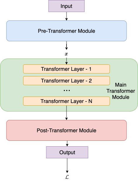
Figure 1: Illustration of the general neural architecture on which our method can be applied.

3 Our Approach

We now follow the analysis framework of T-Fixup Huang et al. (2020), but derive the conditions to bound the gradient updates of the self-attention block in the presence of a pre-trained model. Based on the derivation, we propose a data-dependent initialization strategy for the mixed setup of the new transformers on pre-trained encodings.

3.1 Applicable Architectures

Our analysis applies to the general architecture type illustrated in Figure 1, where the input passes through a pre-transformer, a main transformer, and a post-transformer module before outputting. The pre and post transformer modules can be any architectures that can be stably trained with Adam Kingma and Ba (2014), including MLP, LSTM, CNN, or a pre-trained deep transformer module which can be stably fine-tuned with a learning rate significantly smaller than the main learning rate used for the main transformer module. For this work, we will just consider the case of the main transformer containing only the encoder for simplicity, while our decoder will be an LSTM which can be viewed as part of the post-transformer module. Extending our analysis to include deep transformer decoder is straightforward following the framework of Huang et al. (2020).

We use $f_{e}$ to denote the pre-transformer module ($e$ for pre-trained encoder), and its parameters $\boldsymbol{\theta}_{e}$; similarly $f_{o}$ for post-transformer module ($o$ for output) with parameters $\boldsymbol{\theta}_{o}$. The main transformer module $f_{G}$ is a stack of $L$ transformer blocks, each consisting of a self-attention block and a MLP block. Let $G_{l},l=1,\dots,2N$ denote individual self-attention or MLP layers in the blocks ($G_{l}$’s do not include the skip connections), with parameters $\boldsymbol{\theta}_{l}$ and let $L=2N$, $f_{G}$’s parameters are denoted by $\boldsymbol{\theta}_{G}=\bigcup\limits_{l=1}^{L}\boldsymbol{\theta}_{l}$.

3.2 Theoretical Results for Stable Update

Let the whole model with the output softmax layer(s) and all layer normalization blocks removed be denoted by $f(\cdot;\boldsymbol{\theta})$ and the loss function by $\mathcal{L}$, where $\boldsymbol{\theta}$ are all the learnable parameters. Following Huang et al. (2020), we aim to derive a condition under which, per each SGD update with learning rate $\eta$, the model output changes by $\Theta(\eta)$, i.e. $\lVert\Delta f\rVert=\Theta(\eta)$ where $\Delta f=f(\cdot;\boldsymbol{\theta}-\eta\frac{\partial\mathcal{L}}{\partial\boldsymbol{\theta}})-f(\cdot;\boldsymbol{\theta})$. By Taylor expansion, the SGD update is:

$$\Delta f= \frac{\partial f}{\partial\boldsymbol{\theta}_{o}}\Delta\boldsymbol{\theta}_{o}+\frac{\partial f}{\partial\boldsymbol{\theta}_{G}}\Delta\boldsymbol{\theta}_{G}+\frac{\partial f}{\partial\boldsymbol{\theta}_{e}}\Delta\boldsymbol{\theta}_{e}+$$

$$O(\lVert\boldsymbol{\theta}_{o}\rVert^{2}+\lVert\boldsymbol{\theta}_{G}\rVert^{2}+\lVert\boldsymbol{\theta}_{e}\rVert^{2})$$

$$\phantom{\Delta f}= -\eta(\frac{\partial f_{o}}{\partial\boldsymbol{\theta}_{o}}\frac{\partial f_{o}}{\partial\boldsymbol{\theta}_{o}}^{\top}\frac{\partial\mathcal{L}}{\partial f_{o}}^{\top}+$$

$$\frac{\partial f_{o}}{\partial f_{G}}\frac{\partial f_{G}}{\partial\boldsymbol{\theta}_{G}}\frac{\partial f_{G}}{\partial\boldsymbol{\theta}_{G}}^{\top}\frac{\partial f_{o}}{\partial f_{G}}^{\top}\frac{\partial\mathcal{L}}{\partial f_{o}}^{\top}+$$

$$\frac{\partial f_{o}}{\partial f_{G}}\frac{\partial f_{G}}{\partial f_{e}}\frac{\partial f_{e}}{\partial\boldsymbol{\theta}_{e}}\frac{\partial f_{e}}{\partial\boldsymbol{\theta}_{e}}^{\top}\frac{\partial f_{G}}{\partial f_{e}}^{\top}\frac{\partial f_{o}}{\partial f_{G}}^{\top}\frac{\partial\mathcal{L}}{\partial f_{o}}^{\top})$$

$$+O(\eta^{2})$$ (6)

As assumed in Sec. 3.1, we can stably train $f_{e}$ and $f_{o}$ coupled with $\mathcal{L}$, i.e, $\lVert\frac{\partial\mathcal{L}}{\partial f_{o}}\rVert=\lVert\frac{\partial f_{o}}{\partial\boldsymbol{\theta}_{o}}\rVert=\lVert\frac{\partial f_{e}}{\partial\boldsymbol{\theta}_{e}}\rVert=\lVert\frac{\partial f_{o}}{\partial f_{G}}\rVert=\lVert\frac{\partial f_{G}}{\partial f_{e}}\rVert=\Theta(1)$, we only need to bound the magnitudes of $\frac{\partial f_{G}}{\partial\boldsymbol{\theta}_{G}}$ to bound the overall SGD update. Since what we care is the magnitude of the update as it relates to the depth, we can assume all parameters to be scalars, i.e, $\boldsymbol{q}_{l},\boldsymbol{k}_{l},\boldsymbol{v}_{l},\boldsymbol{w}_{l},\boldsymbol{r}^{k}_{l},\boldsymbol{r}^{v}_{l}$ reduce to scalars $q_{l},k_{l},v_{l},w_{l},r^{k}_{l},r^{v}_{l}\in\mathbb{R}$. The next theorem states the condition under which, $\lVert\frac{\partial f_{G}}{\partial\boldsymbol{\theta}_{G}}\rVert$ is bounded by $\Theta(1)$, achieving the overall $\lVert\Delta f\rVert=\Theta(\eta)$.

Theorem 3.1

Assuming $\lVert\boldsymbol{x}\rVert=\Theta(\mu)$ for some $\mu\gg 1$, then $\lVert\frac{\partial f_{G}}{\partial\boldsymbol{\theta}_{G}}\rVert=\Theta(1)$ if $\lVert v_{l}\rVert=\lVert w_{l}\rVert=\lVert r^{v}_{l}\rVert=\Theta{\left(((4\mu^{2}+2\mu+2)N)^{-\frac{1}{2}}\right)}$ for all encoder layers $l$ in relation-aware transformers; and $\lVert v_{l}\rVert=\lVert w_{l}\rVert=\Theta{\left((4\mu^{2}N)^{-\frac{1}{2}}\right)}$ in the case of vanilla transformers.

The proof is in Appendix A. One important immediate observation is that our scaling as the depth $N$ is to the power of $-1/2$, whereas T-Fixup has a scaling with power of $-1/4$.

While this theorem is all we need for deriving our DT-Fixup approach, it is not immediately intuitive. So next we inspect what it takes to bound the change in a individual layer output $\lVert\Delta G_{l}\rVert$ to $\Theta(\eta/L)$ in each gradient update. This will shine some light on the particular form of the expressions in Theorem 3.1:

Theorem 3.2

Let $\boldsymbol{\boldsymbol{x}}_{l}=[x^{l}_{1},\dots,x^{l}_{n}]$ be the input into $l$-th layer, and assume that $\lVert\partial\mathcal{L}/\partial G_{l}\rVert=\Theta(1)$, i.e. the gradient signal from the layers above is bounded, then $\Delta G_{l}=G_{l}(\boldsymbol{x}_{l}-\eta\frac{\partial\mathcal{L}}{\partial\boldsymbol{x}_{l}};\boldsymbol{\theta}_{l}-\eta\frac{\partial\mathcal{L}}{\partial\mathcal{\boldsymbol{\theta}}_{l}})-G_{l}(\boldsymbol{x}_{l};\boldsymbol{\theta}_{l})$ satisfies $\lVert\Delta G_{l}\rVert=\Theta(\eta/L)$ when for all $i=1,\dots,n$:

$$\begin{split}&2\lVert v_{l}\rVert^{2}\lVert x^{l}_{i}\rVert^{2}+2\lVert v_{l}\rVert\lVert r^{v}_{l}\rVert\lVert x^{l}_{i}\rVert+\lVert r^{v}_{l}\rVert^{2}\\ &+\lVert w_{l}\rVert^{2}(1+2\lVert x^{l}_{i}\rVert^{2})=\Theta(1/N)\\ \end{split}$$ (7)

for relation-aware transformers. Alternatively, in the case of vannilla transformers:

$$\lVert v_{l}\rVert^{2}\lVert x^{l}_{i}\rVert^{2}+\lVert w_{l}\rVert^{2}\lVert x^{l}_{i}\rVert^{2}=\Theta(1/L)$$ (8)

In this case, the proof is straightforward by taking partial derivatives of $G_{l}$ with respect to each parameter, and keep the terms with the lowest powers as they dominate the norm when the scale is smaller than one. Appendix B gives the detailed proof. The insight from this theorem is: if the input $\boldsymbol{x}_{l}$ has the same norm as $\boldsymbol{x}$, setting parameters $v_{l},w_{l},r^{v}_{l}$ to have the same norm and solve the equations would yield the scale factors in Theorem 3.1.

Remark:

In T-Fixup, the corresponding condition to Eq. 8 keeps the term $\lVert v_{l}\rVert^{2}\lVert w_{l}\rVert^{2}$ which is dropped by ours. It is due to the fact that T-Fixup assumes $\lVert x_{i}\rVert$ can be controlled to be the same scale as $v_{l}$ and $w_{l}$, so the lowest power terms (which are dominating the norms here) are the quartic ($4$th power) ones. For us, $\lVert\boldsymbol{x}\rVert$ is treated separately by a constant to be estimated from data, so the lowest power terms are the quadratic ones in $v_{l},w_{l},r^{v}_{l}$ in Eq. 7 and 8, and $\lVert v_{l}\rVert^{2}\lVert w_{l}\rVert^{2}$ are dropped. Another important distinction from T-Fixup is that we assume the estimated $\lVert\boldsymbol{x}\rVert$ to be much larger than the scale of $v_{l}$ and $w_{l}$, unlike the case when they are also controlled to be the same scale. As we will see next, these changes imply our proposed method employs more aggressive scaling for initialization as compared to T-Fixup, and the assumption that $\lVert\boldsymbol{x}\rVert$ has larger scale is satisfied naturally.

3.3 Proposed Method: DT-Fixup

Unlike previous works Zhang et al. (2019b); Huang et al. (2020), appropriate initialization is not enough to ensure Eq. 7 and 8 during the early stage of the training. This is due to the fact that the input $\boldsymbol{x}$ often depends on the pre-trained model weights instead of being initialized by ourselves. Empirically, we observe that the input norm $\lVert\boldsymbol{x}\rVert$ are relatively stable throughout the training but difficulty to control directly by re-scaling. Based on this observation, we treat $\lVert\boldsymbol{x}\rVert$ as a constant and estimate it by a forward pass on all the training examples as $\mu=\max_{j}[\lVert\boldsymbol{x}_{j}\rVert]$. We then use this estimated $\mu$ in the factors of Theorem 3.1 to obtain the scaling needed for initialization. Since parameters of all layers are initialized to the same scale, we drop index $l$ for brevity in this section. In practice, $\mu$ is on the order of $10$ for pre-trained models, hence $v$, $w$ and $r_{i}^{v}$ are naturally two orders of magnitude smaller. DT-Fixup is described as follows:

• Apply Xavier initialization Glorot and Bengio (2010) on all free parameters except loaded weights from the pre-training models;

• Remove the learning rate warm-up and all layer normalization in the transformer layers, except those in the pre-trained transformer;

• Forward-pass on all the training examples to get the max input norm $\mu=\max_{j}[\lVert\boldsymbol{x}_{j}\rVert]$;

• Inside each transformer layer, scale $v,w,r^{v}$ in the attention block and weight matrices in the MLP block by $(N*(4\mu^{2}+2\mu+2))^{-\frac{1}{2}}$ for relation-aware transformer layer; or scale $v,w$ in the attention block and weight matrices in the MLP block by $N^{-\frac{1}{2}}/(2\mu)$ for vanilla transformer layer.

4 Applications

4.1 Text-to-SQL Semantic Parsing

We first apply DT-Fixup on the task of cross-domain Text-to-SQL semantic parsing. Given an unseen schema $\mathcal{S}$ for a database during training, our goal is to translate the natural question $Q$ to the target SQL $T$. The correct prediction depends on the interplay between the questions and the schema structures and the generalization over unseen schemas during inference. As a result, reasoning and structural understanding are crucial to perform well on this task, especially for the more challenging cases. We denote our baseline model as SQL-SP and henceforth.

Implementation.

For modeling Text-to-SQL generation, we adopt the encoder-decoder framework which can be directly fit into the architecture shown in Fig. 1. First, the pre-transformer module $f_{e}$ is a pre-trained language model which embeds the inputs $Q$ and $\mathcal{S}$ into joint representations $\boldsymbol{x}_{i}$ for each column, table $s_{i}\in\mathcal{S}$ and question word $q_{i}\in Q$ respectively. The joint representations are passed into a sequence of $N$ relation-aware transformer layers. The post-transformer module $f_{o}$ is a grammar-guided LSTM decoder, which uses the transformer output $\boldsymbol{y}_{i}$ to predict the target SQL $T$. We follow prior arts Wang et al. (2019a); Guo et al. (2019); Yin and Neubig (2018) to implement SQL-SP. The implementation details and hyperparameter settings are described in Appendix C.

Dataset.

We evaluate SQL-SP on Spider Yu et al. (2018), a complex and cross-domain Text-to-SQL semantic parsing benchmark. The dataset size is relatively small by deep learning standards, with only $10{,}181$ questions and $5{,}693$ queries covering $200$ databases in $138$ domains.

4.2 Logical Reading Comprehension

The second task where we apply DT-Fixup is multi-choice reading comprehension requiring logical reasoning. Given a context, a question and four options, the task is to select the right or most suitable answer. Rather than extracting relevant information from a long context, this task relies heavily on the logical reasoning ability of the models.

Implementation.

On top of the pre-trained encodings of the input context, question and options, a stack of $N$ vanilla transformer layers are added before the final linear layer which gives the predictions. The implementation details and hyperparamter settings are described in Appendix D

Dataset.

We evaluate on ReClor Yu et al. (2020b), a newly curated reading comprehension dataset requiring logical reasoning. The dataset contains logical reasoning questions taken from standardized exams (such as GMAT and LSAT) that are designed for students who apply for admission to graduate schools. Similar to Spider, this dataset is also small, with only $6{,}139$ questions.

5 Experiments

All the experiments in this paper are conducted with a signle 16GB Nvidia P100 GPU.

5.1 Semantic Parsing: Spider Results

As the test set of Spider is only accessible through an evaluation server, most of our analyses are performed on the development set. We use the exact match accuracy on all examples following Yu et al. (2018), which omits evaluation of generated values in the SQL queries.

Model	Dev	Test
RAT-SQL v3 + BERT Wang et al. (2019a)	$69.7$	$65.6$
RAT-SQL + GraPPa Yu et al. (2020a)	$73.4$	$69.6$
RAT-SQL + GAP Shi et al. (2020)	$71.8$	$69.7$
RAT-SQL + GraPPa + GP Zhao et al. (2021)	$72.8$	$69.8$
SGA-SQL + GAP (Anonymous)	$73.1$	$70.1$
RAT-SQL + GraPPa + Adv (Anonymous)	$75.5$	$70.5$
DT-Fixup SQL-SP + RobERTa (ours)	$75.0$	$\mathbf{70.9}$

Table 1: Our accuracy on the Spider development and test sets, as compared to the other approaches at the top of the Spider leaderboard as of May $27$th, 2021.

Model	$N$	Pretrain	Epochs	Acc.
RAT-SQL + BERT	$8$	$\mathbin{\leavevmode\hbox to6.89pt{\vbox to6.89pt{\text{[drawing]}}}}$	$\sim 200$	$69.7$
RAT-SQL + RoBERTa	$8$	$\mathbin{\leavevmode\hbox to6.89pt{\vbox to6.89pt{\text{[drawing]}}}}$	$\sim 200$	$69.6$
RAT-SQL + GraPPa	$8$	$\checkmark$	$\sim 100$	$73.4$
RAT-SQL + GAP	$8$	$\checkmark$	$\sim 200$	$71.8$
SQL-SP + RoBERTa	$8$	$\mathbin{\leavevmode\hbox to6.89pt{\vbox to6.89pt{\text{[drawing]}}}}$	$60$	$66.9$
+ More Epochs	$8$	$\mathbin{\leavevmode\hbox to6.89pt{\vbox to6.89pt{\text{[drawing]}}}}$	$100$	$69.2$
+ DT-Fixup	$8$	$\mathbin{\leavevmode\hbox to6.89pt{\vbox to6.89pt{\text{[drawing]}}}}$	$60$	$73.5$
+ DT-Fixup & More Layers	$24$	$\mathbin{\leavevmode\hbox to6.89pt{\vbox to6.89pt{\text{[drawing]}}}}$	$60$	$75.0$
+ T-Fixup∗ & More Layers	$24$	$\mathbin{\leavevmode\hbox to6.89pt{\vbox to6.89pt{\text{[drawing]}}}}$	$60$	Failed

Table 2: Comparisons with the models leveraging relational transformers on the Spider development set. Pretrain here denotes task-specific pre-training, which leverges additional data and tasks, and is orthorgonal to our contribution. Not only we converge faster and reach better solution, simply training longer from the same baseline cannot close the performance gap. ^∗We drop the constraints on the inputs to allow the application of T-Fixup in the mixed setup.

We present our results on the Spider leaderboard in Table 1, where SQL-SP trained with DT-Fixup outperforms all the other approaches and achieves the new state of the art performance. Notably, the top four submissions on the previous leaderboard are all occupied by models leveraging relation-aware transformers and task-specific pre-training. Table 2 compares our proposed models with the publicly available works. With enough training steps, our baseline model trained with the standard optimization strategy achieves the same level of performance as compared to RAT-SQL. However, models trained with standard optimization strategy obtain much lower performance with the same epochs of training as compared to models trained with DT-Fixup and require more training steps to achieve the best accuracy. At the same time, by adding more relation-aware transformer layers, further gains can be obtained for models trained with DT-Fixup, which achieves the state-of-the-art performance without any task-specific pre-training on additional data sources. As mentioned in Section 2.2, in the mixed setup, there is no way to apply T-Fixup as it was originally proposed. The closest thing to compare is to drop its constraints on the inputs, but training then becomes highly unstable and fails to converge 4 times out of 5 runs. These results demonstrate the necessity and effectiveness of DT-Fixup to improve and accelerate the transformer training for Text-to-SQL parsers.

Model	Easy	Medium	Hard	Extra	All
Dev
RAT-SQL	$86.4$	$73.6$	$62.1$	$42.9$	$69.7$
Bridge (ensemble)	$89.1$	$71.7$	$62.1$	$\mathbf{51.8}$	$71.1$
DT-Fixup SQL-SP	$91.9$	$\mathbf{80.9}$	$60.3$	$48.8$	$75.0$
Test
RAT-SQL	$83.0$	$71.3$	$58.3$	$38.4$	$65.6$
Bridge (ensemble)	$85.3$	$73.4$	$59.6$	$40.3$	$67.5$
DT-Fixup SQL-SP	$87.2$	$\mathbf{77.5}$	$60.9$	$\mathbf{46.8}$	$70.9$

Table 3: Breakdown of Spider accuracy by hardness.

Table 3 shows the accuracy of our best model as compared to other approaches with different level of hardness defined by Yu et al. (2018). We can see that a large portion of the improvement of our model comes from the medium level on both dev and test set. Interestingly, while our model obtains similar performance for the extra hard level on the dev set, our model performs significantly better on the unseen test set. As most of the extra hard cases involves implicit reasoning steps and complicated structures, it shows that our proposed models possess stronger reasoning and structural understanding ability, yielding better generalization over unseen domains and database schemas.

5.2 Reading Comprehension: ReClor Results

Model	Dev	Test
no extra layers∗ Yu et al. (2020b)	$62.6$	$55.6$
no extra layers	$63.6$	$56.2$
$4$ extra layers	$66.2$	$58.2$
$4$ extra layers + DT-Fixup	$\mathbf{66.8}$	$\mathbf{61.0}$

Table 4: Our accuracy on ReClor. Star^∗ is the best baseline model result reported in Yu et al. (2020b) without using the additional RACE dataset Lai et al. (2017).

$N$	Standard	DT-Fixup
Spider
2	$69.47\pm 0.30$	$70.73\pm 0.18$
4	$70.04\pm 0.33$	$72.22\pm 0.61$
8	$66.86\pm 0.16$	$73.24\pm 0.51$
16	$20.44\pm 1.11$	$73.52\pm 0.47$
24	$19.37\pm 0.16$	$73.79\pm 0.49$
32	$19.57\pm 0.43$	$73.02\pm 0.52$
ReClor
4	$64.05\pm 0.44$	$64.31\pm 0.68$
8	$56.96\pm 6.12$	$65.31\pm 0.62$
16	$27.10\pm 1.50$	$65.68\pm 1.12$

Table 5: Ablation on the number of transformer layers $N$. The means and standard deviations are reported based on $5$ runs with different random seeds.

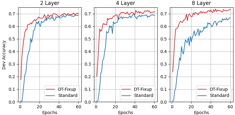
Figure 2: Validation curves on Spider for models trained with different settings.

	Base	Shallow	Deep
False neg.	39	35	42
Column err. only	51	60	53
Sketch err. only	92	83	77
Both err.	124	105	88
All	306	283	260

Table 6: Failures in each category.

Figure 3: Error breakdown on examples where all models are wrong.

Figure 4: Error breakdown on examples where any model is wrong.

For ReClor, we choose the best model in Yu et al. (2020b) as the baseline which employs a linear classifier on top of RoBERTa. From the results presented in Table 4, we can see that simply stacking additional vanilla transformer layers outperforms the baseline and adding DT-Fixup further improves the accuracy, which ranks the second on the public leaderboard at the time of this submission. The result further validates the benefit of adding extra transformer layers and the effectiveness of DT-Fixup.

5.3 Ablation Studies

For fair comparisons and better understanding, we conduct multiple sets of ablation with the same architecture and implementation to validate the advantages of DT-Fixup over the standard optimization strategy. Note that, the batch sizes in our experiments are relatively small (16 for Spider and 24 for ReClor) due to the size of the pre-trained models, while batch sizes for masked language modelling Liu et al. (2019b) and machine translation Huang et al. (2020) are commonly larger than $1024$.

Deeper Models.

As we can see from Table 5, the standard optimization strategy fails completely to train deep transformers whose depths are larger than $8$ on both Spider and ReClor, showing that it struggles to properly train the transformer model as the depth increases. At the same time, DT-Fixup can successfully train deeper transformers up to $32$ layers and consistently achieves better performance than models trained by the standard optimization strategy with the same depth on both Spider and ReClor. With DT-Fixup, deep models generally achieve better performance than the shallow ones even there are only thousands of training examples. It contradicts the common belief that increasing depth of the transformer model is helpful only when there are enough training data.

Faster Convergence.

Demonstrated by the validation curves on Spider plotted in Figure 2, models trained with DT-Fixup converges to the same level of performance much faster than models trained with the standard optimization strategy. While standard optimization strategy struggles as the models become deeper, DT-Fixup can keep the model training smooth, showing that DT-Fixup can effectively accelerate the convergence of the transformer training, especially for the deep ones.

Batch Sizes When Dataset Size is Small.

As shown in Table 7, increasing batch size on Spider from 16 to 120, the average performance from five runs drops from 73.24 to 71.08 and the gap with the standard training approach becomes much narrower. It empirically verifies that large-batch training has a negative impact on the generalization when the dataset size is small, confirming the need to stablize small batch training.

Model	Batch Size	Acc
$8$ extra layers + Standard	16	$69.60\pm 0.40$
$8$ extra layers + DT-Fixup	16	$73.24\pm 0.51$
$8$ extra layers + DT-Fixup	120	$71.08\pm 0.37$

Table 7: Ablation on the batch sizes for the Spider dataset. To enable large-batch training, we implement the trick of gradient accumulation at the expense of training speed. The means and standard deviations are reported based on 5 runs with different random seeds.

5.4 Source of the Improvements

From the results on the Spider benchmark, we can see significant improvements by applying DT-Fixup and increasing the depth of the transformer model. However, why and where they help Text-to-SQL semantic parsing are still unclear. As an attempt to answer these questions, we investigate into the predicted results from three variants of our proposed model: Baseline, the best model ($N=4$) trained with the standard training approach; Shallow, a shallow model ($N=4$) trained with DT-Fixup; Deep, our best model ($N=24$) trained with DT-Fixup, which is much deeper.

To better understand the models’ behavior, we manually examine all the failed cases predicted by these models and classify the errors into four categories: 1) Correct: equivalent in meaning but with different SQL syntax (e.g., ORDER BY X LIMIT 1 and SELECT MIN(X)); 2) Column: the SQL structure is correct but there existed mispredicted columns; 3) Sketch: the SQL structure is predicted different from the ground truth, while the aligned column prediction are correct; 4) Both: there exist both sketch and column errors in the prediction. Table 6 presents the overall statistics of our error analysis. Due to logically equivalent queries, there are a number of false negatives for all three models, confirming that the current Spider evaluation metric is not ideal. At first glance, the improvements by applying DT-Fixup and increasing the depth seem to come from correcting Sketch and Both errors, while the three models make similar number of Column only errors. It provides evidence that applying DT-Fixup and increasing the depth can help the transformer model handle hard examples which are mispredicted completely (errors in Both category) by the baseline model. Typically, correct predictions on these hard examples require a certain level of reasoning and structural understanding ability.

Fine-grained Error Analysis. In order to better understand the errors made, we look into the composition of error types by each model on mistaken examples common to all models, as well as on examples where at least one model is wrong. In Fig. 3-4, “Column” means “proportion with column errors” (i.e., Column or Both); “Sketch” means “proportion with sketch errors” (i.e., Sketch or Both). There are $190$ examples mispredicted by all the three models and $387$ examples which at least one of the three models mispredict. Fig. 3-4 exclude false negatives due to equivalent logic queries, we can see the real improvements from the deep model are even more significant than what the exact match accuracy shows. Furthermore, among the common mistakes to all three models, the deep model has a much smaller proportion in the sketch mistakes which usually involve more logic and structure understanding. Some of column mistakes are due to missing domain knowledge or common sense, which is harder to improve without external data or knowledge. This shows that even among the failed cases, deeper transformer model can make more reasonable predictions.

6 Related Work

Many research efforts have been devoted to understanding the training and improving the optimization of the transformer models. In particular, transformer models often fail to learn unless a gradual learning rate warm-up is applied at the beginning of training. Chen et al. (2018); Nguyen and Salazar (2019); Wang et al. (2019b) noticed a performance gap due to layer normalization, and introduced various architecture changes as remedy. Zhang et al. (2019b, a); Liu et al. (2020) proposed initialization schemes to stabilize training, allowing either to remove layer normalization or learning rate warmup. Liu et al. (2019a) demonstrated the instability of the Adam optimizer during early stages of optimization. Based on these results, Huang et al. (2020) proposed a weight initialization schema for the transformer that eliminates the need for layer normalization and warmup completely.

7 Conclusion

Despite the broad applications of the transformer model, it struggles to perform well for some NLP tasks with limited training data. In this work, we propose a theoretically justified optimization strategy DT-Fixup to train deeper transformer model with improved generalization and faster convergence speed on small datasets, which is generally applicable to different neural architectures. On two important tasks, Text-to-SQL semantic parsing and logical reading comprehension that require reasoning and structural understanding, applying DT-Fixup achieves SOTA or near-SOTA results by simplying using extra transformer layers on top of the pre-trained models. Such observations suggest even boarder applicability of deeper transformers.

Appendix A Full Proof

Theorem 3.1

Assuming $\lVert\boldsymbol{x}\rVert=\Theta(\mu)$ for some $\mu\gg 1$, then $\lVert\frac{\partial f_{G}}{\partial\boldsymbol{\theta}_{G}}\rVert=\Theta(1)$ if $\lVert v_{l}\rVert=\lVert w_{l}\rVert=\lVert r^{v}_{l}\rVert=\Theta{\left(((4\mu^{2}+2\mu+2)N)^{-\frac{1}{2}}\right)}$ for all encoder layers $l$ in relational transformers; and $\lVert v_{l}\rVert=\lVert w_{l}\rVert=\Theta{\left((4\mu^{2}N)^{-\frac{1}{2}}\right)}$ in the case of vanilla transformers.

Proof. First, let’s inspect the feedforward pass through the transformer blocks, which have nonlinear layers $G_{l}$’s and skip connections: $\boldsymbol{x}_{1}=\boldsymbol{x};~{}~{}~{}~{}\boldsymbol{x}_{2}=\boldsymbol{x}_{1}+G_{1}(\boldsymbol{x}_{1},\boldsymbol{\theta}_{1});~{}~{}\ldots;~{}~{}\boldsymbol{x}_{l+1}=\boldsymbol{x}_{l}+G_{l}(\boldsymbol{x}_{l},\boldsymbol{\theta}_{l})$ For $l\%2=1$ (i.e. odd layers), $G_{l}$ is a (relational) self-attention layer, whereas for even layers, $G_{l}$ is a MLP layer. Using $\stackrel{{\scriptstyle\mathclap{\mbox{$\Theta$}}}}{{=}}$ to denote bounded in norm as in Huang et al. (2020), then at initialization:

$$\boldsymbol{x}_{l+1} \stackrel{{\scriptstyle\mathclap{\mbox{$\Theta$}}}}{{=}}\boldsymbol{x}_{l}+v_{l}w_{l}\boldsymbol{x}_{l}+w_{l}r^{v}_{l}\quad\quad\quad\quad\text{For relational self-attention}$$ (9)

$$\boldsymbol{x}_{l+1} \stackrel{{\scriptstyle\mathclap{\mbox{$\Theta$}}}}{{=}}\boldsymbol{x}_{l}+v_{l}w_{l}\boldsymbol{x}_{l}\quad\quad\quad\quad\quad\quad\quad\text{For vanilla self-attention and MLP}$$ (10)

This is due to the fact that the probability from softmax sums to one, so does not alter the overall norm; at initialization, values are at the linear identity range of the nonlinearities. Therefore, for all three types of layers: $\frac{\partial\boldsymbol{x}_{l+1}}{\partial\boldsymbol{x}_{l}}\stackrel{{\scriptstyle\mathclap{\mbox{$\Theta$}}}}{{=}}1+v_{l}w_{l}$ and $\frac{\partial G_{l}}{\partial\boldsymbol{x}_{l}}\stackrel{{\scriptstyle\mathclap{\mbox{$\Theta$}}}}{{=}}v_{l}w_{l}$. And for relational self-attention: $\frac{\partial\boldsymbol{x}_{l+1}}{\partial\boldsymbol{\theta}_{l}}=\frac{\partial G_{l}}{\partial\boldsymbol{\theta}_{l}}\stackrel{{\scriptstyle\mathclap{\mbox{$\Theta$}}}}{{=}}[w_{l}\boldsymbol{x}_{l},v_{l}\boldsymbol{x}_{l}+r^{v}_{l},w_{l},\boldsymbol{0}]$, where $\boldsymbol{0}$ are due to $q$, $k$, $\boldsymbol{r}^{k}$ which appear only inside the softmax and do not asymptotically affect the norm. And for vanilla self-attention and MLP, $\frac{\partial\boldsymbol{x}_{l+1}}{\partial\boldsymbol{\theta}_{l}}=\frac{\partial G_{l}}{\partial\boldsymbol{\theta}_{l}}\stackrel{{\scriptstyle\mathclap{\mbox{$\Theta$}}}}{{=}}[w_{l}\boldsymbol{x}_{l},v_{l}\boldsymbol{x}_{l},\boldsymbol{0}]$. Next, let’s look at $\frac{\partial f_{G}}{\partial\boldsymbol{\theta}_{G}}=[\frac{\partial f_{G}}{\partial\boldsymbol{\theta}_{1}},\ldots,\frac{\partial f_{G}}{\partial\boldsymbol{\theta}_{l}},\ldots,\frac{\partial f_{G}}{\partial\boldsymbol{\theta}_{L}}]$. First note that:

$$f_{G}(\boldsymbol{x},\boldsymbol{\theta}_{G})=\boldsymbol{x}_{1}+G_{1}(\boldsymbol{x}_{1},\boldsymbol{\theta}_{1})+G_{2}(\boldsymbol{x}_{2},\boldsymbol{\theta}_{2})+\ldots+G_{L}(\boldsymbol{x}_{2},\boldsymbol{\theta}_{L})$$ (11)

Working backwards, for the last layer, $\frac{\partial f_{G}}{\partial\boldsymbol{\theta}_{L}}\!=\!\frac{\partial G_{L}}{\partial\boldsymbol{\theta}_{L}}$. For $\frac{\partial f_{G}}{\partial\boldsymbol{\theta}_{l}}$, terms with index lower than $l$ vanish, so:

$${\partial f_{G}}/{\partial\boldsymbol{\theta}_{l}} ={\partial G_{l}}/{\partial\boldsymbol{\theta}_{l}}+{\partial G_{l+1}}/{\partial\boldsymbol{x}_{l+1}}{\partial\boldsymbol{x}_{l+1}}/{\partial\boldsymbol{\theta}_{l}}+\ldots+{\partial G_{L}}/{\partial\boldsymbol{x}_{L}}{\partial\boldsymbol{x}_{L}}/{\partial\boldsymbol{x}_{L-1}}\ldots{\partial\boldsymbol{x}_{l+1}}/{\partial\boldsymbol{\theta}_{l}}$$ (12)

$$\stackrel{{\scriptstyle\mathclap{\mbox{$\Theta$}}}}{{=}}\left(1+v_{l+1}w_{l+1}+\ldots+v_{L}w_{L}(1+v_{L-1}w_{L-1})\ldots(1+v_{l+1}w_{l+1})\right){\partial G_{l}}/{\partial\boldsymbol{\theta}_{l}}$$ (13)

Assuming $v_{1}\stackrel{{\scriptstyle\mathclap{\mbox{$\Theta$}}}}{{=}}v_{2}\ldots\stackrel{{\scriptstyle\mathclap{\mbox{$\Theta$}}}}{{=}}v_{L}$ and $w_{1}\stackrel{{\scriptstyle\mathclap{\mbox{$\Theta$}}}}{{=}}w_{2}\ldots\stackrel{{\scriptstyle\mathclap{\mbox{$\Theta$}}}}{{=}}w_{L}$, and both $\ll 1$, then the above reduces to:

$${\partial f_{G}}/{\partial\boldsymbol{\theta}_{l}}\stackrel{{\scriptstyle\mathclap{\mbox{$\Theta$}}}}{{=}}(1+(L-l)v_{l}w_{l}){\partial G_{l}}/{\partial\boldsymbol{\theta}_{l}}$$ (14)

Recall that we want to bound $\frac{\partial f_{G}}{\partial\boldsymbol{\theta}_{G}}\frac{\partial f_{G}}{\partial\boldsymbol{\theta}_{G}}^{\top}={\textstyle\sum}_{l}\frac{\partial f_{G}}{\partial\boldsymbol{\theta}_{l}}\frac{\partial f_{G}}{\partial\boldsymbol{\theta}_{l}}^{\top}$. For vanilla self-attention or MLP layers:

$$\frac{\partial f_{G}}{\partial\boldsymbol{\theta}_{l}}\frac{\partial f_{G}}{\partial\boldsymbol{\theta}_{l}}^{\top}\stackrel{{\scriptstyle\mathclap{\mbox{$\Theta$}}}}{{=}}\left(\lVert w_{l}\rVert^{2}\lVert\boldsymbol{x}_{l}\rVert^{2}+\lVert v_{l}\rVert^{2}\lVert\boldsymbol{x}_{l}\rVert^{2}\right)(1+(L-l)\lVert v_{l}\rVert\lVert w_{l}\rVert)^{2}$$ (15)

And for relational self-attention:

$$\frac{\partial f_{G}}{\partial\boldsymbol{\theta}_{l}}\frac{\partial f_{G}}{\partial\boldsymbol{\theta}_{l}}^{\top}\!\!\stackrel{{\scriptstyle\mathclap{\mbox{$\Theta$}}}}{{=}}\!\!\left(\lVert w_{l}\rVert^{2}\lVert\boldsymbol{x}_{l}\rVert^{2}\!\!+\!\!\lVert v_{l}\rVert^{2}\lVert\boldsymbol{x}_{l}\rVert^{2}\!\!+\!\!2\lVert v_{l}\rVert\lVert\boldsymbol{x}_{l}\rVert\lVert r^{v}_{l}\rVert\!\!+\!\!\lVert r^{v}_{l}\rVert^{2}\!\!+\!\!\lVert w_{l}\rVert^{2}\right)(1\!\!+\!\!(L\!-\!l)\lVert v_{l}\rVert\lVert w_{l}\rVert)^{2}$$ (16)

At initialization, we want $v_{l}$, $w_{l}$, $r^{v}_{l}$ of all layers to have the same norm, i.e. $\lVert v_{l}\rVert\stackrel{{\scriptstyle\mathclap{\mbox{$\Theta$}}}}{{=}}\lVert w_{l}\rVert\stackrel{{\scriptstyle\mathclap{\mbox{$\Theta$}}}}{{=}}\lVert r^{v}_{l}\rVert\stackrel{{\scriptstyle\mathclap{\mbox{$\Theta$}}}}{{=}}\lVert v_{j}\rVert\stackrel{{\scriptstyle\mathclap{\mbox{$\Theta$}}}}{{=}}\lVert w_{j}\rVert\stackrel{{\scriptstyle\mathclap{\mbox{$\Theta$}}}}{{=}}\lVert r^{v}_{j}\rVert$ for all $l$ and $j$, so denoting them using $\xi$. And recall that $N$ is the number of transformer blocks, with each block containing two layers, so that $2N=L$. So we have:

$$\frac{\partial f_{G}}{\partial\boldsymbol{\theta}_{G}}\frac{\partial f_{G}}{\partial\boldsymbol{\theta}_{G}}^{\top} \!\!\stackrel{{\scriptstyle\mathclap{\mbox{$\Theta$}}}}{{=}}\!{\textstyle\sum}_{l\%2=0}\!\left(\!2\xi^{2}\lVert\boldsymbol{x}_{l}\rVert^{2}\!\right)\left(1\!+\!(L\!-\!l)\xi^{2}\right)\!+\!{\textstyle\sum}_{l\%2=1}\!\left(\!2\xi^{2}\lVert\boldsymbol{x}_{l}\rVert^{2}\!+\!2\xi^{2}\lVert\boldsymbol{x}_{l}\rVert\!+\!2\xi^{2}\!\right)\!\left(\!1\!+\!(L\!-\!l)\xi^{2}\right)$$

$$\stackrel{{\scriptstyle\mathclap{\mbox{$\Theta$}}}}{{=}}{\textstyle\sum}^{N}_{l=1}\left(4\xi^{2}\lVert\boldsymbol{x}_{l}\rVert^{2}+2\xi^{2}\lVert\boldsymbol{x}_{l}\rVert+2\xi^{2}\right)(1+(2N-l)\xi^{2})$$ (17)

Similarly if $f_{G}$ is vanilla transformer instead of a relational one, we have:

$$\frac{\partial f_{G}}{\partial\boldsymbol{\theta}_{G}}\frac{\partial f_{G}}{\partial\boldsymbol{\theta}_{G}}^{\top} \stackrel{{\scriptstyle\mathclap{\mbox{$\Theta$}}}}{{=}}{\textstyle\sum}^{N}_{l=1}\left(4\xi^{2}\lVert\boldsymbol{x}_{l}\rVert^{2}\right)(1+(2N-l)\xi^{2})$$ (18)

The only variable that still depends on $l$ is $\boldsymbol{x}_{l}$, which by expanding the recursion in Eq. 9-10, gives:

$$\boldsymbol{x}_{l} \stackrel{{\scriptstyle\mathclap{\mbox{$\Theta$}}}}{{=}}(1+\xi^{2})^{l}\boldsymbol{x}\stackrel{{\scriptstyle\mathclap{\mbox{$\Theta$}}}}{{=}}(1+l\xi^{2}+\Theta(\xi^{4}))\boldsymbol{x}\quad\quad\quad\quad\quad\quad\quad\quad\quad\text{For vanillla transformer}$$ (19)

$$\boldsymbol{x}_{l} \stackrel{{\scriptstyle\mathclap{\mbox{$\Theta$}}}}{{=}}(1+\xi^{2})^{l}\boldsymbol{x}+l/2\xi^{2}\stackrel{{\scriptstyle\mathclap{\mbox{$\Theta$}}}}{{=}}(1+l\xi^{2}+\Theta(\xi^{4}))\boldsymbol{x}+l/2\xi^{2}\quad\text{For relational transformer}$$ (20)

Now let $\lVert\boldsymbol{x}\rVert\stackrel{{\scriptstyle\mathclap{\mbox{$\Theta$}}}}{{=}}\mu$ , and we have assumed that $\mu\gg 1$, which is very common for output of pre-trained encoders, and due to the high dimensionality. And let

$$\xi=\left(N(4\mu^{2}+2\mu+2)\right)^{-\frac{1}{2}}$$ (21)

Then substituting it into Eq. 19-20, we have $\boldsymbol{x}_{l}\stackrel{{\scriptstyle\mathclap{\mbox{$\Theta$}}}}{{=}}\boldsymbol{x}$ for all types of layers. Similarly, plugging Eq. 21 into the expression $(1+(2N-l)\xi^{2})$ in Eq. 17 yields $(1+(2N-l)\xi^{2})\stackrel{{\scriptstyle\mathclap{\mbox{$\Theta$}}}}{{=}}1$, together with $\boldsymbol{x}_{l}\stackrel{{\scriptstyle\mathclap{\mbox{$\Theta$}}}}{{=}}\boldsymbol{x}$, and Eq. 21, Eq. 17 becomes:

$$\frac{\partial f_{G}}{\partial\boldsymbol{\theta}_{G}}\frac{\partial f_{G}}{\partial\boldsymbol{\theta}_{G}}^{\top}\stackrel{{\scriptstyle\mathclap{\mbox{$\Theta$}}}}{{=}}{\textstyle\sum}^{N}_{l=1}\frac{4\mu^{2}}{N\left(4\mu^{2}+2\mu+2\right)}+\frac{2\mu}{N\left(4\mu^{2}+2\mu+2\right)}+\frac{2}{N\left(4\mu^{2}+2\mu+2\right)}\stackrel{{\scriptstyle\mathclap{\mbox{$\Theta$}}}}{{=}}{\textstyle\sum}^{N}_{l=1}1/N=\Theta(1)$$

This concludes the proof for relational transformers. For vanilla transformers, with $\xi=\left(N(4\mu^{2})\right)^{-\frac{1}{2}}$, and following the same steps, but plugging into Eq. 18, we have $\frac{\partial f_{G}}{\partial\boldsymbol{\theta}_{G}}\frac{\partial f_{G}}{\partial\boldsymbol{\theta}_{G}}^{\top}\stackrel{{\scriptstyle\mathclap{\mbox{$\Theta$}}}}{{=}}1$. Q.E.D.

Appendix B Proof of Theorem 3.2

For brevity, we drop the layer index. But for the relation embeddings, for clarity, we will consider the individual components of $\boldsymbol{r}^{v},\boldsymbol{r}^{k}$ instead of considering the scalar case.

Proof. We will focus the self-attention layer, as the skip connection and MLP layers are analyzed in Huang et al. (2020). As mentioned in the main text, since what we care is the magnitude of the update, we assume $d_{x}=1$ and drop layer index $l$ without loss of generality. In this case, the projection matrices $\boldsymbol{q},\boldsymbol{k},\boldsymbol{v},\boldsymbol{w}$ reduce to scalars $q,k,v,w\in\mathbb{R}$. The input $\boldsymbol{x}$ and the relational embeddings $\boldsymbol{r}^{k},\boldsymbol{r}^{v}$ are $n\times 1$ vectors. For a single query input $x^{\prime}\in\boldsymbol{x}$, the attention layer (without skip connection) is defined as follows:

$$G(x^{\prime})=\text{softmax}\left(\frac{1}{\sqrt{d_{x}}}x^{\prime}q(k\boldsymbol{x}+\boldsymbol{r}^{k})^{\top}\right)(\boldsymbol{x}v+\boldsymbol{r}^{v})w={\textstyle\sum}_{i=1}^{n}\frac{e^{x^{\prime}q(kx_{i}+r_{i}^{k})}}{{\textstyle\sum}_{j=1}^{n}e^{x^{\prime}q(kx_{j}+r_{j}^{k})}}(x_{i}v+r_{i}^{v})w$$

Note that we are abusing the notation and take $G$ to be just the self-attention layer output here. Let $s_{i}=e^{x^{\prime}q(kx_{i}+r_{i}^{k})}/{\textstyle\sum}_{j=1}^{n}e^{x^{\prime}q(kx_{j}+r_{j}^{k})}$ and $\delta_{ij}=1$ if $i=j$ and 0 otherwise, we can get:

$$\begin{split}{\partial G}/{\partial k}&=x^{\prime}qw{\textstyle\sum}_{i=1}^{n}(x_{i}v+r_{i}^{v})s_{i}\left(x_{i}-{\textstyle\sum}_{j=1}^{n}x_{j}s_{j}\right)\\ {\partial G}/{\partial q}&=x^{\prime}w{\textstyle\sum}_{i=1}^{n}(x_{i}v+r_{i}^{v})s_{i}\left(kx_{i}+r_{i}^{k}-{\textstyle\sum}_{j=1}^{n}(kx_{j}+r_{j}^{k})s_{j}\right)\\ {\partial G}/{\partial r_{i}^{k}}&=x^{\prime}qw\left(-(x_{i}v+r_{i}^{v})s_{i}+{\textstyle\sum}_{j=1}^{n}(x_{j}v+r_{j}^{v})s_{j}\right)~{};~{}~{}~{}{\partial G}/{\partial v}=w{\textstyle\sum}_{i=1}^{n}x_{i}s_{i}\\ {\partial G}/{\partial w}&={\textstyle\sum}_{i=1}^{n}(x_{i}v+r_{i}^{v})s_{i}~{};~{}~{}~{}{\partial G}/{\partial r_{i}^{v}}=ws_{i}~{};~{}~{}~{}{\partial G}/{\partial x_{i}}=vws_{i}+w{\textstyle\sum}_{j=1}^{n}{\partial s_{j}}/{\partial x_{i}}(x_{j}v+r_{j}^{v})\end{split}$$

When $x_{i}\neq x^{\prime}$, we have: $\frac{\partial s_{j}}{\partial x_{i}}=s_{j}(\delta_{ij}-s_{i})x^{\prime}qk$; When $x_{i}=x^{\prime}$, we have: $\frac{\partial s_{j}}{\partial x_{i}}=q\left((1+\delta_{ij})kx_{i}+r_{i}^{k}\right)s_{j}-{\textstyle\sum}_{t=1}^{n}q\left((1+\delta_{it})kx_{t}+r_{t}^{k}\right)s_{j}s_{t}$ Using Taylor expansion, we get that the SGD update $\Delta G$ is proportional to the magnitude of the gradient:

$$\begin{split}\Delta G&=-\eta\frac{\partial\mathcal{L}}{\partial G}\left(\frac{\partial G}{\partial k}\frac{\partial G}{\partial k}^{\top}+\frac{\partial G}{\partial q}\frac{\partial G}{\partial q}^{\top}+\frac{\partial G}{\partial v}\frac{\partial G}{\partial v}^{\top}+\frac{\partial G}{\partial w}\frac{\partial G}{\partial w}^{\top}\right.\\ &\left.+{\textstyle\sum}_{i=1}^{n}\frac{\partial G}{\partial r_{i}^{k}}\frac{\partial G}{\partial r_{i}^{k}}^{\top}+{\textstyle\sum}_{i=1}^{n}\frac{\partial G}{\partial r_{i}^{v}}\frac{\partial G}{\partial r_{i}^{v}}^{\top}+{\textstyle\sum}_{i=1}^{n}\frac{\partial G}{\partial x_{i}}\frac{\partial G}{\partial x_{i}}^{\top}\right)+O(\eta^{2})\end{split}$$

By the assumption that $\lVert\eta\frac{\partial\mathcal{L}}{\partial G}\rVert=\Theta(\eta)$, we need to bound the term inside the main parentheses by $\Theta(1/L)$. The desired magnitude $\Theta(1/L)$ is smaller than 1 so terms with lower power are dominating. With $s_{i}\geq 0$ and ${\textstyle\sum}s_{i}=1$, the following terms have the lowest power inside the main parentheses:

$$\begin{split}\frac{\partial G}{\partial v}\frac{\partial G}{\partial v}^{\top}&=w^{2}({\textstyle\sum}_{i=1}^{n}x_{i}s_{i})^{2}=\Theta(\lVert w\rVert^{2}\lVert x_{i}\rVert^{2}),\ i=1,\dots,n\\ \frac{\partial G}{\partial w}\frac{\partial G}{\partial w}^{\top}&=({\textstyle\sum}_{i=1}^{n}(x_{i}v+r_{i}^{v})s_{i})^{2}=\Theta(\lVert v\rVert^{2}\lVert x_{i}\rVert^{2})+2\Theta(\lVert v\rVert\lVert r_{i}^{v}\rVert\lVert x_{i}\rVert)+\Theta(\lVert r_{i}^{v}\rVert^{2}),\ i=1,\dots,n\\ {\textstyle\sum}_{i=1}^{n}\frac{\partial G}{\partial r_{i}^{v}}\frac{\partial G}{\partial r_{i}^{v}}^{\top}&=w^{2}{\textstyle\sum}_{i=1}^{n}s_{i}^{2}=\Theta(\lVert w\rVert^{2}).\\ \end{split}$$

For the MLP layer, all terms related to $r_{i}^{v}$ disappear, including the single $\Theta(\lVert w\rVert^{2})$ in the last row. By combining the update norm terms from both the self-attention and the MLP layers give the result. Q.E.D. Note: The above theorem and analysis applies to a single layer, not the whole transformer module of many layers. In order to derive the scaling factor, one needs ensure that the output scale for each block is bounded by its input scale. This indeed holds for our scheme, but the complete proof is in Sec. A.

Appendix C Implementation Details of SQL-SP

Given a schema $\mathcal{S}$ for a relational database, our goal is to translate the natural question $Q$ to the target SQL $T$. Here the question $Q=q_{1}\dots q_{\lvert Q\rvert}$ is a sequence of words, and the schema $\mathcal{S}=\{s_{1},\dots,s_{\lvert\mathcal{S}\rvert}\}$ consists of tables and their columns. $s\in\mathcal{S}$ can be either a table name or a column name containing words $s_{i,1},\dots,s_{i,\lvert s_{i}\rvert}$. Following Wang et al. (2019a), a directed graph $\mathcal{G}=\langle\mathcal{V},\mathcal{E}\rangle$ can be constructed to represent the relations between the inputs. Its nodes $\mathcal{V}=Q\cup\mathcal{S}$ include question tokens (each labeled with a corresponding token) and the columns and tables of the schema (each labeled with the words in its name). The edges $\mathcal{E}$ are defined following Wang et al. (2019a). The target SQL $T$ is represented as an abstract syntax tree in the context-free grammar of SQL.

C.1 Encoder

Following Wang et al. (2019a); Guo et al. (2019), our pre-transformer module $f_{e}$ leverages pre-trained language models to obtain the input $X$ to the main transformer module. First, the sequence of words in the question $Q$ are concatenated with all the items (either a column or a table) in the schema $\mathcal{S}$. In order to prevent our model from leveraging potential spurious correlations based on the order of the items, the items in the schema are concatenated in random order during training. We feed the concatenation into the pre-trained model and extract the last hidden states $\boldsymbol{x}_{i}^{(q)}$ and $\boldsymbol{h}_{i}=\boldsymbol{h}_{i,1},\dots,\boldsymbol{h}_{i,\lvert s_{i}\rvert}$ for each word in $Q$ and each item in $\mathcal{S}$ respectively. For each item $s_{i}$ in the schema, we run an additional bidirectional LSTM (BiLSTM) Hochreiter and Schmidhuber (1997) over the hidden states of the words in its name $\boldsymbol{h}_{i}$. We then add the average hidden state and the final hidden state of the BiLSTM as the schema representations $\boldsymbol{x}_{i}^{(s)}$. $X$ is the set of all the obtained representations from $Q\cup\mathcal{S}$: $X=(\boldsymbol{x}_{1}^{(q)},\dots,\boldsymbol{x}_{\lvert Q\rvert}^{(q)},\boldsymbol{x}_{1}^{(s)},\dots,\boldsymbol{x}_{\lvert\mathcal{S}\rvert}^{(s)}).$ Along with the relational embeddings $\boldsymbol{r}^{k},\boldsymbol{r}^{v}$ specified by $\mathcal{G}$, $X$ is passed into the main transformer module.

C.2 Schema Linking

The goal of schema linking is to identify the implicit relations between $Q$ and $\mathcal{S}$. The relations are defined by whether there exist column/table references in the question to the corresponding schema columns/tables, given certain heuristics. Following Wang et al. (2019a), possible relations for each $(i,j)$ where $x_{i}\in Q,x_{j}\in\mathcal{S}$ (or vice versa) can be ExactMatch, PartialMatch, or NoMatch, which are based on name-based linking. Depending on the type of $x_{i}$ and $x_{j}$, the above three relations are further expanded to four types: Question-Column, Question-Table, Column-Question, or Table-Question. We also use the value-based linking from Wang et al. (2019a) and Guo et al. (2019) to augment the ExactMatch relation by database content and external knowledge.

C.3 Decoder

For our decoder (as the post-transformer module) $f_{o}$, we employ a transition-based abstract syntax decoder following Yin and Neubig (2018). It requires a transition system to converts between the surface SQL and a AST-tree constructing action sequences, and can ensure grammarticality of generation. The neural model then predicts the action sequences. There are three types of actions to generate the target SQL $T$, including (i) ApplyRule which applies a production rule to the last generated node; (ii) Reduce which completes a leaf node; (iii) SelectColumn which chooses a column from the schema. For our transition system, each column is attached with their corresponding table so that the tables in the target SQL $T$ can be directly inferred from the predicted columns. As a result, action SelectTable can be omitted from the generation. Formally, the generation process can be formulated as $\Pr(T|\mathcal{Y})=\prod_{t}\Pr(a_{t}|a_{<t},\mathcal{Y})$ where $\mathcal{Y}$ is the outputs of the last layer of the relational transformers. We use a parent-feeding LSTM as the decoder. The LSTM state is updated as $\boldsymbol{m}_{t},\boldsymbol{h}_{t}=f_{\text{LSTM}}([\boldsymbol{a}_{t-1}\|\boldsymbol{z}_{t-1}\|\boldsymbol{h}_{p_{t}}\|\boldsymbol{a}_{p_{t}}\|\boldsymbol{n}_{p_{t}}],\boldsymbol{m}_{t-1},\boldsymbol{h}_{t-1})$, where $\boldsymbol{m}_{t}$ is the LSTM cell state, $\boldsymbol{h}_{t}$ is the LSTM output at step $t$, $\boldsymbol{a}_{t-1}$ is the action embedding of the previous step, $\boldsymbol{z}_{t-1}$ is the context feature computed using multi-head attention on $\boldsymbol{h}_{t-1}$ over $\mathcal{Y}$, $p_{t}$ is the step corresponding to the parent AST node of the current node, and $\boldsymbol{n}$ is the node type embedding. For ApplyRule[R], we compute $\Pr(a_{t}=\texttt{ApplyRule[R]}|a_{<t},y)=\text{softmax}_{R}(g(\boldsymbol{z}_{t}))$ where $g(\cdot)$ is a $2$-layer MLP. For SelectColumn, we use the memory augmented pointer net Guo et al. (2019).

C.4 Regularization

Besides using dropout Srivastava et al. (2014) employed on $X$ and $\boldsymbol{z}_{t}$ to help regularize the model, we further apply uniform label smoothing Szegedy et al. (2016) on the objective of predicting SelectColumn. Formally, the cross entropy for a ground-truth column $c^{*}$ we optimize becomes: $(1-\epsilon)*\log p(c^{*})+{\epsilon}/{K}*{\textstyle\sum}_{c}\log p(c)$, where $K$ is the number of columns in the schema, $\epsilon$ is the weight of the label smoothing term, and $p(\cdot)\triangleq\Pr(a_{t}=\texttt{SelectColumn}[\cdot]|a_{<t},y)$.

C.5 Experiment Configuration

We choose RoBERTa Liu et al. (2019b) as the pre-trained language models. A sequence of 24 relation-aware transformer layers are stacked on top of $f_{e}$. The Adam optimizer Kingma and Ba (2014) with the default hyperparameters is used to train the model with an initial learning rate $\eta$ of $4\times 10^{-4}$. $\eta$ is annealed to $0$ with $4\times 10^{-4}(1-steps/max\_steps)^{0.5}$. A separate learning rate is used to fine-tune the RoBERTa by multiplying $\eta$ a factor of $8\times 10^{-3}$. The BiLSTM to encode the schema representations has hidden size $128$ per direction. For each transformer layer, $d_{x}=d_{z}=256$, $H=8$ and the inner layer dimension of the position-wise MLP is $1024$. For the decoder, we use action embeddings of size $128$, node type embeddings of size of $64$, and LSTM hidden state of size $512$. We apply dropout rate of $0.6$ on the input to the relational transformers $X$ and the context representation $\boldsymbol{z}_{t}$. The weight of the label smoothing term is set to be $0.2$. We use a batch size of $16$ and train $60$ epochs (around $25,000$ steps). During inference, beam search is used with beam size as $5$. Most of the hyperparameters are chosen following Wang et al. (2019a). We only tune the learning rate ($4\times 10^{-4}$ to $8\times 10^{-4}$ with step size $1\times 10^{-4}$), dropout ($0.3$, $0.4$, $0.5$, $0.6$), the weight of the label smoothing $\epsilon$ ($0.0$, $0.1$, $0.2$) by grid search. The average runtime is around 30 hours and the number of parameters is around 380 millions.

Appendix D Implementation Details for Logical Reading Comprehension

We build on the code by Yu et al. (2020b) and use it for evaluation. For each example, the encoder embeds the input context, question and options which are then passed to the linear layer for classification. The exact input format to the encoder is “$\langle s\rangle$ Context $\langle/s\rangle\langle/s\rangle$ Question $||$ Option $\langle pad\rangle\dots$”, where “$||$” denotes concatenation. The linear layer uses the embedding of the first token $\langle s\rangle$ for classification.

D.1 Experimental Configuration

RoBERT is chosen as the pre-trained model, and we stack $4$ transformer layers on top. The Adam optimizer Kingma and Ba (2014) with $\epsilon=10^{-6}$ and betas of $(0.9,0.98)$ is used. The learning rate to finetune RoBERTa is $1\times 10^{-5}$ while the learning rate for the additional transformer layers is $3\times 10^{-4}$. For all models in our ablation study, the learning rate for the additional transformer layers is $1\times 10^{-4}$. The learning rate is annealed linearly to $0$ with weight decay of $0.01$. We use a batch size of $24$ and fine-tune for $12$ epochs. For each transformer layer, $d_{x}=d_{z}=1024$, $H=8$ and the inner layer dimension of the position-wise MLP is $2048$. We use dropout rate of $0.4$ on the input to the additional transformer layers and $0.1$ for the linear layer. We follow the hyperparameters used in Yu et al. (2020b) for the pretrained language model. For the additional transformer layers, we only tune the dropout values $(0.3,0.4,0.5,0.6)$. The average runtime is around 6 hours and the number of parameters is around 39 millions.

References

- Ba et al. (2016) Jimmy Lei Ba, Jamie Ryan Kiros, and Geoffrey E Hinton. 2016. Layer normalization. arXiv preprint arXiv:1607.06450.
- Chen et al. (2018) Mia Xu Chen, Orhan Firat, Ankur Bapna, Melvin Johnson, Wolfgang Macherey, George Foster, Llion Jones, Mike Schuster, Noam Shazeer, Niki Parmar, et al. 2018. The best of both worlds: Combining recent advances in neural machine translation. In Proceedings of the 56th Annual Meeting of the Association for Computational Linguistics (Volume 1: Long Papers), pages 76–86.
- Devlin et al. (2018) Jacob Devlin, Ming-Wei Chang, Kenton Lee, and Kristina Toutanova. 2018. Bert: Pre-training of deep bidirectional transformers for language understanding. arXiv preprint arXiv:1810.04805.
- Glorot and Bengio (2010) Xavier Glorot and Yoshua Bengio. 2010. Understanding the difficulty of training deep feedforward neural networks. In Proceedings of the thirteenth international conference on artificial intelligence and statistics, pages 249–256.
- Guo et al. (2019) Jiaqi Guo, Zecheng Zhan, Yan Gao, Yan Xiao, Jian-Guang Lou, Ting Liu, and Dongmei Zhang. 2019. Towards complex text-to-sql in cross-domain database with intermediate representation. ACL.
- Hochreiter and Schmidhuber (1997) Sepp Hochreiter and Jürgen Schmidhuber. 1997. Long short-term memory. Neural computation, 9(8):1735–1780.
- Huang et al. (2020) Xiao Shi Huang, Felipe Pérez, Jimmy Ba, and Maksims Volkovs. 2020. Improving transformer optimization through better initialization. ICML.
- Keskar et al. (2016) Nitish Shirish Keskar, Dheevatsa Mudigere, Jorge Nocedal, Mikhail Smelyanskiy, and Ping Tak Peter Tang. 2016. On large-batch training for deep learning: Generalization gap and sharp minima. arXiv preprint arXiv:1609.04836.
- Kingma and Ba (2014) Diederik P Kingma and Jimmy Ba. 2014. Adam: A method for stochastic optimization. arXiv preprint arXiv:1412.6980.
- Lai et al. (2017) Guokun Lai, Qizhe Xie, Hanxiao Liu, Yiming Yang, and Eduard Hovy. 2017. RACE: Large-scale ReAding comprehension dataset from examinations. In Proceedings of the 2017 Conference on Empirical Methods in Natural Language Processing, pages 785–794, Copenhagen, Denmark. Association for Computational Linguistics.
- Lan et al. (2019) Zhenzhong Lan, Mingda Chen, Sebastian Goodman, Kevin Gimpel, Piyush Sharma, and Radu Soricut. 2019. Albert: A lite bert for self-supervised learning of language representations. arXiv preprint arXiv:1909.11942.
- Liu et al. (2019a) Liyuan Liu, Haoming Jiang, Pengcheng He, Weizhu Chen, Xiaodong Liu, Jianfeng Gao, and Jiawei Han. 2019a. On the variance of the adaptive learning rate and beyond. arXiv preprint arXiv:1908.03265.
- Liu et al. (2020) Liyuan Liu, Xiaodong Liu, Jianfeng Gao, Weizhu Chen, and Jiawei Han. 2020. Understanding the difficulty of training transformers. EMNLP.
- Liu et al. (2019b) Yinhan Liu, Myle Ott, Naman Goyal, Jingfei Du, Mandar Joshi, Danqi Chen, Omer Levy, Mike Lewis, Luke Zettlemoyer, and Veselin Stoyanov. 2019b. Roberta: A robustly optimized bert pretraining approach. arXiv preprint arXiv:1907.11692.
- Nguyen and Salazar (2019) Toan Q Nguyen and Julian Salazar. 2019. Transformers without tears: Improving the normalization of self-attention. arXiv preprint arXiv:1910.05895.
- Popel and Bojar (2018) Martin Popel and Ondřej Bojar. 2018. Training tips for the transformer model. The Prague Bulletin of Mathematical Linguistics, 110(1):43–70.
- Radford et al. (2019) Alec Radford, Jeffrey Wu, Rewon Child, David Luan, Dario Amodei, and Ilya Sutskever. 2019. Language models are unsupervised multitask learners. OpenAI Blog, 1(8):9.
- Shaw et al. (2018) Peter Shaw, Jakob Uszkoreit, and Ashish Vaswani. 2018. Self-attention with relative position representations. In Proceedings of the 2018 Conference of the North American Chapter of the Association for Computational Linguistics: Human Language Technologies, Volume 2 (Short Papers), pages 464–468.
- Shi et al. (2020) Peng Shi, Patrick Ng, Zhiguo Wang, Henghui Zhu, Alexander Hanbo Li, Jun Wang, Cicero Nogueira dos Santos, and Bing Xiang. 2020. Learning contextual representations for semantic parsing with generation-augmented pre-training. arXiv preprint arXiv:2012.10309.
- Srivastava et al. (2014) Nitish Srivastava, Geoffrey Hinton, Alex Krizhevsky, Ilya Sutskever, and Ruslan Salakhutdinov. 2014. Dropout: a simple way to prevent neural networks from overfitting. The journal of machine learning research, 15(1):1929–1958.
- Szegedy et al. (2016) Christian Szegedy, Vincent Vanhoucke, Sergey Ioffe, Jon Shlens, and Zbigniew Wojna. 2016. Rethinking the inception architecture for computer vision. In Proceedings of the IEEE conference on computer vision and pattern recognition, pages 2818–2826.
- Vaswani et al. (2017) Ashish Vaswani, Noam Shazeer, Niki Parmar, Jakob Uszkoreit, Llion Jones, Aidan N Gomez, Łukasz Kaiser, and Illia Polosukhin. 2017. Attention is all you need. In Advances in neural information processing systems, pages 5998–6008.
- Wang et al. (2019a) Bailin Wang, Richard Shin, Xiaodong Liu, Oleksandr Polozov, and Matthew Richardson. 2019a. Rat-sql: Relation-aware schema encoding and linking for text-to-sql parsers. arXiv preprint arXiv:1911.04942.
- Wang et al. (2019b) Qiang Wang, Bei Li, Tong Xiao, Jingbo Zhu, Changliang Li, Derek F Wong, and Lidia S Chao. 2019b. Learning deep transformer models for machine translation. In Proceedings of the 57th Annual Meeting of the Association for Computational Linguistics, pages 1810–1822.
- Xu et al. (2019) Hongfei Xu, Qiuhui Liu, Josef van Genabith, Deyi Xiong, and Jingyi Zhang. 2019. Lipschitz constrained parameter initialization for deep transformers. arXiv preprint arXiv:1911.03179.
- Yin and Neubig (2018) Pengcheng Yin and Graham Neubig. 2018. Tranx: A transition-based neural abstract syntax parser for semantic parsing and code generation. arXiv preprint arXiv:1810.02720.
- Yu et al. (2020a) Tao Yu, Chien-Sheng Wu, Xi Victoria Lin, Bailin Wang, Yi Chern Tan, Xinyi Yang, Dragomir Radev, Richard Socher, and Caiming Xiong. 2020a. Grappa: Grammar-augmented pre-training for table semantic parsing. arXiv preprint arXiv:2009.13845.
- Yu et al. (2018) Tao Yu, Rui Zhang, Kai Yang, Michihiro Yasunaga, Dongxu Wang, Zifan Li, James Ma, Irene Li, Qingning Yao, Shanelle Roman, et al. 2018. Spider: A large-scale human-labeled dataset for complex and cross-domain semantic parsing and text-to-sql task. In Proceedings of the 2018 Conference on Empirical Methods in Natural Language Processing, pages 3911–3921.
- Yu et al. (2020b) Weihao Yu, Zihang Jiang, Yanfei Dong, and Jiashi Feng. 2020b. Reclor: A reading comprehension dataset requiring logical reasoning. arXiv preprint arXiv:2002.04326.
- Zhang et al. (2019a) Biao Zhang, Ivan Titov, and Rico Sennrich. 2019a. Improving deep transformer with depth-scaled initialization and merged attention. In Proceedings of the 2019 Conference on Empirical Methods in Natural Language Processing and the 9th International Joint Conference on Natural Language Processing (EMNLP-IJCNLP), pages 897–908.
- Zhang et al. (2019b) Hongyi Zhang, Yann N Dauphin, and Tengyu Ma. 2019b. Fixup initialization: Residual learning without normalization. ICLR.
- Zhao et al. (2021) Liang Zhao, Hexin Cao, and Yunsong Zhao. 2021. Gp: Context-free grammar pre-training for text-to-sql parsers. arXiv preprint arXiv:2101.09901.